Optimizing Extreme Learning Machines Using Chains of Salps for Efficient Android Ransomware Detection


1
King Abdullah II School for Information Technology, The University of Jordan, Amman 11942, Jordan
2
Computer Science Department, Prince Sultan University, Riyadh 11586, Saudi Arabia
3
Computer Science Department, The University of Jordan, Amman 11942, Jordan
4
Department of Computer Science, Faculty of Information Technology, Zarqa University, Zarqa 13132, Jordan
*
Author to whom correspondence should be addressed.
Appl. Sci. 2020, 10(11), 3706; https://doi.org/10.3390/app10113706
Submission received: 17 April 2020
/
Revised: 14 May 2020
/
Accepted: 19 May 2020
/
Published: 27 May 2020
(This article belongs to the Special Issue Intelligence Systems and Sensors)
Abstract
:Nowadays, smartphones are an essential part of people’s lives and a sign of a contemporary world. Even that smartphones bring numerous facilities, but they form a wide gate into personal and financial information. In recent years, a substantial increasing rate of malicious efforts to attack smartphone vulnerabilities has been noticed. A serious common threat is the ransomware attack, which locks the system or users’ data and demands a ransom for the purpose of decrypting or unlocking them. In this article, a framework based on metaheuristic and machine learning is proposed for the detection of Android ransomware. Raw sequences of the applications API calls and permissions were extracted to capture the ransomware pattern of behaviors and build the detection framework. Then, a hybrid of the Salp Swarm Algorithm (SSA) and Kernel Extreme Learning Machine (KELM) is modeled, where the SSA is used to search for the best subset of features and optimize the KELM hyperparameters. Meanwhile, the KELM algorithm is utilized for the identification and classification of the apps into benign or ransomware. The performance of the proposed (SSA-KELM) exhibits noteworthy advantages based on several evaluation measures, including accuracy, recall, true negative rate, precision, g-mean, and area under the curve of a value of 98%, and a ratio of 2% of false positive rate. In addition, it has a competitive convergence ability. Hence, the proposed SSA-KELM algorithm represents a promising approach for efficient ransomware detection.
1. Introduction
Day by day the number of mobile users exceptionally increases and approximately surpasses the 2.5 billion users worldwide [1]. Android is an operating system manufactured using a Linux-based kernel for cellular phones. Recently, it has been considerably popular for smartphones and the Internet of things devices. Even that, it constitutes a favorable environment for malicious applications to disseminate. Malware is a malicious software accesses and hijacks computer or mobile systems, which eventually could damage, steal, encrypt, or disable the system files or data. Malware software comes in different forms such as spyware, ransomware, trojans, worms, viruses, or others. In [2], it had been reported that a single family of mobile ransomware had a negative effect on one million Android users in one month. Ransomware is a kind of malware software that hinders the user with the infected mobile from accessing their data due to either data encryption or device locking, while the attacker waits for a ransom to decrypt the data or unlock the cellular device. Even that its source code is available online but safeguarding against it is hard [3]. Indeed, it is a requirement to design an effective ransomware detection approach.
In the literature, the research community developed different solutions to combat ransomware, such as the use of honeypots, or the use of statistical methods. These approaches are facing challenges such as the high false positive rates, or a limited capacity to detect complex, persistently-evolved ransomware attacks [4,5] ideally before the files are encrypted or the system is damaged. Artificial intelligence, machine learning, and deep learning tools have been elucidating very efficient abilities in capturing hidden patterns of information and inferring useful knowledge that would be capable of unraveling intricate attacks. Machine learning approaches that are devoted to malware detection rely on utilizing a learning algorithm that learns discriminating characteristics of a malicious application and successfully classifies it into a malware application or a benign application. However, the constantly increasing number of mobile applications as well as the rapid growth of malware families, in particular, the ransomware; have led to the requirement of developing a more resilient and robust detection algorithm.
The performance of machine learning algorithms is significantly affected by various factors; such as the settings of the hyperparameters or the presence of irrelevant, redundant features. Thereby, developing an efficient malware detection algorithm requires handling the variable, high-dimensional attributes of malwares, while setting the hyperparameters properly. A fundamental preprocessing step during modeling a machine learning algorithm is the feature selection. Feature selection is concerned with removing the irrelevant redundant features which deteriorate the performance of a learning algorithm. Three major approaches are identified for performing feature selection; filter-based, wrapper-based, and embedded-based approaches. Filter methods assess and rank the features independently from the learning algorithm like the correlation filter. Whereas, the wrapper methods depend on a learning algorithm to evaluate potential subsets of features and score the best one that has the highest prediction power. Embedded approaches search for the best features during the training procedure as in the genetic programming algorithm [6].
Feature selection is a discrete optimization problem that attempts to find an optimal value (“optimum”) of an objective function based on the optimal subset of features. Primarily, optimization problems can optimize the respective set of features, as well as searching for the best values of the hyperparameters. A well-regarded type of optimization algorithms is the metaheuristic algorithms which demonstrated an eminent ability in finding feasible solutions in a reasonable amount of time [7].
Metaheuristic algorithms are a kind of random and global search algorithms that evolved to tackle hard-optimization problems in a feasible amount of time. For example, feature selection in classification problems is a typical optimization problem where the objective is to find the minimal best set of features as well as to maximize the classification performance. In other words, given a dataset with (n) number of features yields a large search space of potential features subsets, which increases the complexity of the search process, yet becomes more challenging. Remarkably, metaheuristics had shown prominent capacity in approaching hard-optimization problems due to the capability of performing stochastically local and global searches, interchangeably [8,9,10]. Owing to their random natural behavior, they can traverse various areas in the search space, which promotes solutions diversity and quality. An efficient metaheuristic strategy can regularize evenly between searching globally which is known as exploration or diversification, and locally that is referred to as exploitation or intensification. The Exploration and exploitation search schemes are two principal components of metaheuristic algorithms. Exploration corresponds to producing more diversified solutions that reside in less-visited regions in the search space, as well as it avoids the trapping in a local best solution during the search of global optima. Whereas, exploitation implies to search at the local regions that potentially can create good solutions [7].
Nature-inspired algorithms are a type of metaheuristics that are inspired by several natural phenomena including the evolution and natural selection, the cooperative foraging behaviors, or physical and chemical observations in ecological systems. Typically, nature-inspired algorithms are widely used to solve optimization, modeling, and simulation problems in various fields of science. Generally, they are grouped into two taxonomies; the population-based or the trajectory-based. Population-based evolutionary algorithms are more common for performing exploration and search at a global scale, which is contrary to the trajectory-based algorithms that are more suitable for exploiting the current region and search at a local scale. In consequence, the Salp Swarm Algorithm (SSA) is a relatively new population-based algorithm that is inspired by the foraging behavior of salps in deep oceans [11]. SSA algorithm has proved efficacy in dealing with feature selection problems and hyperparameter tuning [12,13].
In this work, we propose a hybrid machine learning model that combines a modified recent swarm intelligent algorithm which is the SSA algorithm with Kernel Extreme Learning Machine (KELM) for Android ransomware detection. The SSA is modified at the level of the swarm structure and the binarization level. The SSA is used to optimize the hyperparameters of the KELM and feature selection, simultaneously. The proposed model is developed for the task of Android ransomware detection based on features that are extracted from 1000 Android applications’ permissions and API calls. The goal is to detect Android ransomware with high prediction power with the minimum possible number of features.
This paper is structured into six major sections, as follows: the next Section 2 reviews recent works in the area of ransomware detection methods and techniques. Section 3 briefly describes the algorithms used in the proposed detection model. Section 4 presents the proposed classification framework covering an architectural overview, dataset description, the proposed SSA-KELM classification system, and the evaluation measures. The experiments and results are discussed in Section 5. Finally, the main findings and conclusion of this work are given in Section 6.
2. Related Works
In recent years, the ransomware attacks of mobile devices have grown dramatically, which lead to a significant need for developing efficient protective and defensive solutions. However, in the literature, several research studies have concerned with tackling the problem of ransomware detection over cellular or mobile networks and in particular over Android mobile networks. This section discusses thoroughly the recently proposed solutions for the detection of such a serious problem.
One of the early implementations of Android ransomware recognition is HelDroid that developed by Andronio et al. [14]. HelDroid used three criteria for the detection of ransomware, where one of them is a text classification technique to detect either ransomware or scareware, However, HelDroid is an offline detection method that is computationally expensive. While in [15], implemented a ransomware detection called GreatEatlon, which consists of multiple detection modules like the text analysis and encryption detection methods. Even that GreatEatlon showed improved and faster identification of Android ransomware, but it is computationally demanding and relies heavily on the text classifier that might be broken by string encryption. Nonetheless, Song et al. [16] implemented a system to identify ransomware and goodware by observing continuously the conducted processes. While interestingly in [17], Gharib and Ghorbani designed a hybrid of static-based and dynamic-based environment for the detection of ransomware on Android, which is called Dna-Droid. The static part of the system depended on the classification of texts and images, as well as, analyzing the APIs calls and permissions. On the other hand, the dynamic part used a deep learning approach (autoencoder neural network) to detect the presence of ransomware by analyzing and classifying system call sequences. However, the Dna-Droid was not tested on real ransomware samples as well as did not consider the scalability issues. The process of scanning Android apps to conduct both static and dynamic analysis was detailed in [18,19]. Nonetheless, Chen et al. [20] deployed a ransomware detection system (RansomProper) that observes the execution of applications and the usage of user interface (UI) widgets to extract valuable features and perform real-time detection. Although, RansomProper showed a high-performance ability in detecting the malicious encryption of files but failed to achieve relatively low execution time.
Furthermore, [21], Canfora et al. [21] introduced the use of Hidden Markov Models (HMM) and structural entropy for the detection of Android malware. The integration of HMM is for the recognition of the malware application, while the structural entropy is for identifying the malware family. Additionally, Chen et al. [22] designed StormDroid system which is a machine learning-oriented approach for the detection of Android malware. StormDroid extracted four types of features; sequences and dynamic features, as well as API calls and permissions. However, the authors did not consider the influence of the number of collected features in the performance of the proposed approach.
In [23], Ahmadi et al. [23] proposed IntelliAV that is an anti-malware system for Android. IntelliAV stands mainly on extracting a set of features (e.g. permissions, APIs, intents, and statistical features), which then are used by a TensorForest algorithm to differentiate the malware class from the benign class. However, the authors stated some limitations of the proposed system as the inability to detect malware that uses javascript. Moreover, Garcia et al. [24] proposed a machine learning approach for Android malware detection (RevealDroid). RevealDroid extracts the features from applications’ binaries and APIs, which then used by the support vector machines (SVMs) for the recognition of the malware. Meanwhile, the classification and regression trees (CART) algorithm was used for the identification of the malware family. Markedly, RevealDroid achieved high performance in terms of accuracy, efficiency, and resilience. However, since this work collected a high-dimensional dataset; studying the effect of features on the algorithm performance will be of great importance. In [25], Cimitile et al. [25] proposed TALOS, which is a ransomware detector for Android based on formal detection methods. TALOS used logical rules to spot the ransomware. Even though it obtained high detection accuracy, it requires long execution time. Su et al. [26] designed an approach for the detection of Android locker-ransomware. Where Su et al. [26] extracted six sets of discriminating features including background behaviors like the permissions and system calls, as well as text features. The model was trained by using an ensemble of classical machine learning algorithms, which showed efficient performance capability.
Sharma et al. [27] created a RansomwareElite android application for the detection of ransomware. It monitors the device for any malicious textual codes, or permissions using the natural language processing toolkit (NLTK). However, the authors did not perform real experiments with reliable performance results. In essence, a more recent study [28] has proposed a multi-stage framework for android ransomware detection. The designed approach used natural language processing techniques and machine learning to extract multiple types of features, and then detect the ransomware. In which, the logistic regression classifier with the term frequency-inverse document frequency for feature representation achieved the best detection accuracy. Even the authors relied only on the accuracy measure to compare the algorithms, but other evaluation measures, as well as the time requirements, are essential.
In [29], Scalas et al. proposed a learning-based approach for the detection of ransomware for Android devices. In which, the proposed approach relied on the application programming interface (APIs) information to recognize ransomware attacks and the generic malware. An R-PackDroid package is implemented which showed competitive results in comparison with previously suggested solutions. Even that it merely depends on the APIs information, which might affect its reliability in case of large-scale and online detection frameworks. Remarkably, Alzahrani and Alghazzawi [30] performed a survey of deep learning techniques for the detection of Android ransomware. The authors stated that there are very few research studies concerned with the deployment of deep learning during the period (2014-2019). In addition, most of the used deep learning models were based on autoencoders and deep belief networks. However, roughly speaking, most of them have long execution time which makes them impractical. Alsoghyer and Almomani [31,32] conducted a machine learning approach for Android ransomware detection. Mainly, the features extracted statistically (API calls, permissions, operation code) and dynamically (user interaction and phone events). Using several evaluation metrics to assess the used machine learning methods; the results showed very effective accuracy (96.5%) in comparison with state-of-the-art methods.
Since ransomware attacks are exponentially growing with various characteristics; a more resilient approach is a demand to overcome their variable signatures. In [33], a two-level system is implemented for the detection of Android ransomware. The first level tracks Windows API calls sequences to build a Marcov model that captures the attributes of ransomwares. Whereas, the second level is a random forest classifier to detect the ransomware. Impressively, the proposed approach achieved promising results regarding the false positive rate and the false negative rate. However, the authors did not report how much the proposed approach is demanding, where the resources and time requirements are fundamental for automatic ransomware detection. In [34], Abdullah et al. proposed a machine learning approach for dynamically capturing the features and detecting Android ransomware. The features were dynamically extracted and analyzed using systems calls, where the results exhibited a very low false positive rate.
3. Preliminaries
3.1. Salp Swarm Algorithm
The SSA algorithm is a stochastic swarm intelligence algorithm developed by Mirjalili et al. in [11]. Essentially, the SSA algorithm inspired by the foraging behavior of salps and their structural spiral-chains in deep oceans. Salps are barrel-shaped marine organisms that return to the family of Salpidae. They gather in a chain like a spiral or a wheel, swim synchronously, and cooperate to find the food. Figure 1 shows an example of a chain of salps. The striking insight of the SSA algorithm is the collective and foraging behavior of salps swarm in the sea.
Typically, the SSA is a metaheuristic and global optimizer that capable of handling complex, constrained, and unconstrained problems. As well as, it showed promising performance in various fields, such as feature selection [12,13,35,36,37], optimization problems in engineering [9,11], and other applications [10,38]. A salp’s chain consists of a leader salp and follower salps. The leader salp is responsible for searching for a food source, while the follower salps, progressively, follow the leading salp for the sake of reaching a food source.
The SSA algorithm is a search and population-based metaheuristic algorithm. Certainly, search algorithms have a known search space, a search criterion, and an evaluation function. Hence, the SSA algorithm has a population of salps (individuals) that represent potential random solutions and belong to a predefined search space. A population of salps (X) is composed of a leader salp and () follower salps, which is expressed by a 2-dimensional matrix as in Equation (1). (N) is the number of salps in the swarm, and (d) is the dimension of a salp.
The objective of the salps is to find the optimal source food (F). In order to formulate the mathematical model of salps chain; each salp is characterized by a position vector. Thus, the leader salp () is illustrated by Equation (2), where () is the position of the source food in the jth dimension, () and () are two random numerical values in the range [0,1], and (, ) are the upper and lower bounds of the dimension, respectively.
whereas, () is a controlling coefficient and decreases over the course of iterations. Typically, () plays a crucial role in balancing between diversification and intensification, which hinders the algorithm from trapping in local optima or experiencing a premature convergence. Equation (3) describes the behavior of () parameter, in which, (l) is the current iteration, and (L) is the predefined total number of iterations.
The follower salps adjust their positions iteratively as expressed in Equation (4), where . Algorithm 1 presents the pseudo-code of the SSA algorithm.
The SSA algorithm initializes the population by the randomly generated salps. Thereby, each salp in the chain is assessed based on an objective (or fitness) criterion. The procedure of the algorithm, in an iterative way, modify the positions of all salps (Equation (4)), evaluate them, and assign the fittest salp as the source food (F). At each iteration, the parameter () is modified, while each dimension of the leader salp is adjusted regarding Equation (2). Eventually, the algorithm stops when a terminating condition is satisfied.
| Algorithm 1 Pseudo-code of the SSA algorithm |
|
Create an initial population of salps while (Stopping condition is not satisfied) do Measure the fitness values of all salps Set the food source F Update using Equation (3) for (each salp ()) do if () then Adjust the leader by Equation (2) else if then Adjust the followers by Equation (4) end if end for Update each salp to obey the and bounds Remove the salps that are out of the search space. end while Return F |
3.2. Kernel Extreme Learning Machine
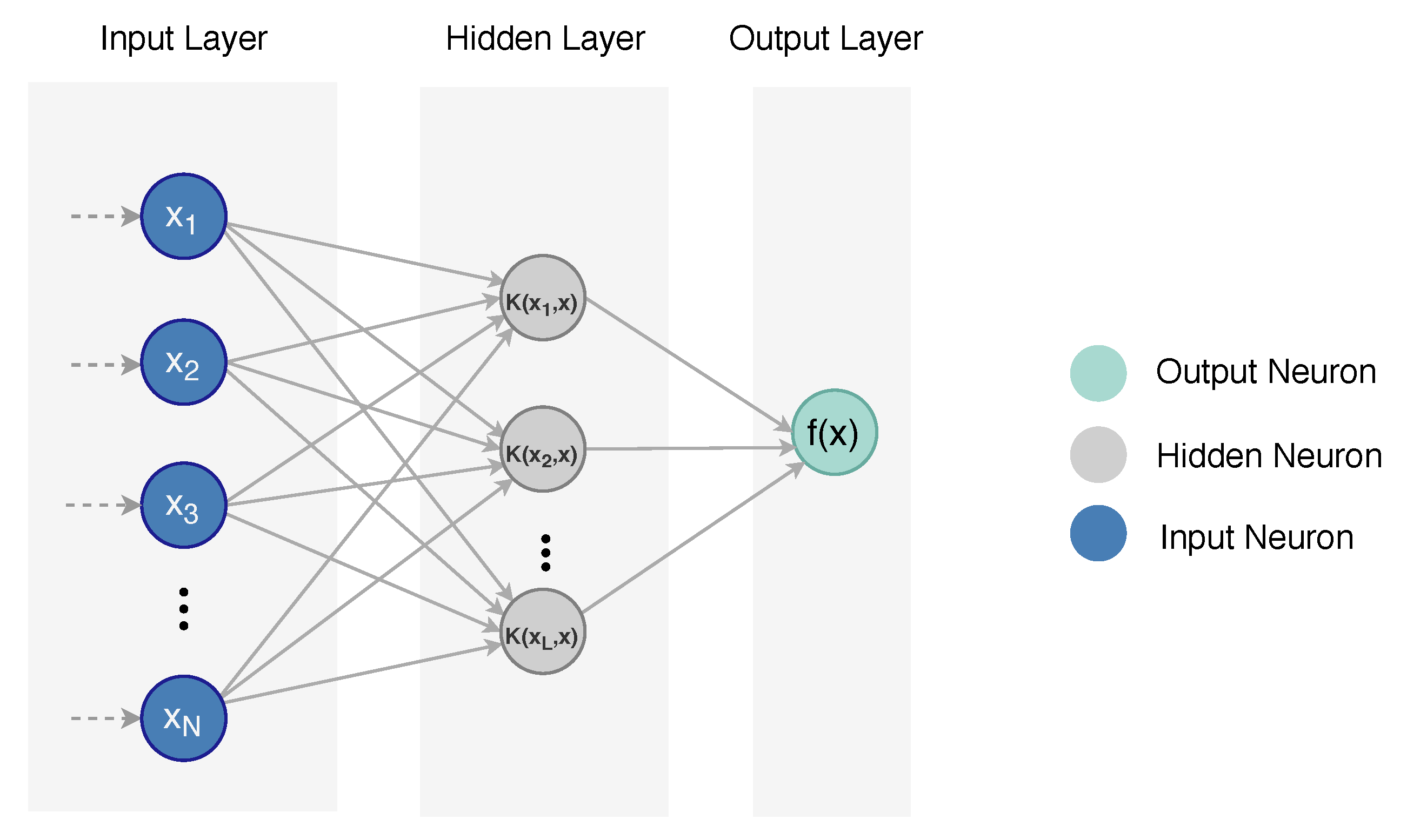
The KELM was proposed by Huang et al. [39] as a type of the classical Extreme Learning Machine (ELM) [40]. The main motivation for ELM was to overcome the drawbacks of traditional gradient descent methods for training feedforward neural networks (FFNN). ELM incorporates three steps to train the FFNN algorithm. It starts by initially assigning the input weights and the hidden biases of the FFNN randomly, then it calculates the hidden layer output matrix and finally, in one step it determines the output weights using Moore–Penrose (MP) generalized inverse. Recently, there have been studies that utilized other approaches such as evolutionary computing for training ELMs and optimizing their structures. In the KELM algorithm, Huang et al. utilized the idea of the kernel function in ELM.
The output of ELM with L hidden neurons can be given as shown in Equation (5), knowing that we have a training sample set .
where is the output weight vectors that connect the hidden layer to the output layer. () is the weights vector that connects the (jth) hidden node to the input layer, and () is the bias of the (jth) node. () is the output matrix of the hidden layer with respect to the input (x). ELM algorithm tries to minimize the training error and at the same time minimizes the norm of the output weights . The optimization function of ELM can be expressed as follows.
In which, . (C) is the factor that controls the trade-off between the training error and the norm of the output weights. While, (H) is the matrix of the hidden layer (Equation (7)).
whereas, is the target matrix of the training data. The output of ELM based on N (number of training samples) and L (the number of hidden neurons) is defined as presented in Equation (8).
In the case that the user does not know the feature mapping matrix (H), a kernel matrix of ELM, which is called kernel function mapping can be used by applying Equations (9)–(10).
where is the kernel function. By applying Equations (8) and (9), Equation (5) can be written as in (Equation (10)).
The kernel function that is commonly used in the KELM is the radial basis function (RBF), also known as the Gaussian kernel function. RBF is defined as follows:
The two crucial parameters are the regularization factor C and the kernel parameter . C is used to get better adjustment between the error minimization and the model complexity to enhance the generalization performance. is used to define the mapping from the input space to the high dimensional feature space.
The general structure of the KELM is shown in Figure 2
4. Proposed Framework for Android Ransomware Detection
This section exhibits the developed classification framework that targets ransomware over Android devices. The section introduces a general architecture for ransomware detection, describes the collected dataset, presents the design issues of the proposed classification approach (SSA-KELM), as well as its procedure. In addition, it points out to the utilized evaluation measures.
4.1. Overview
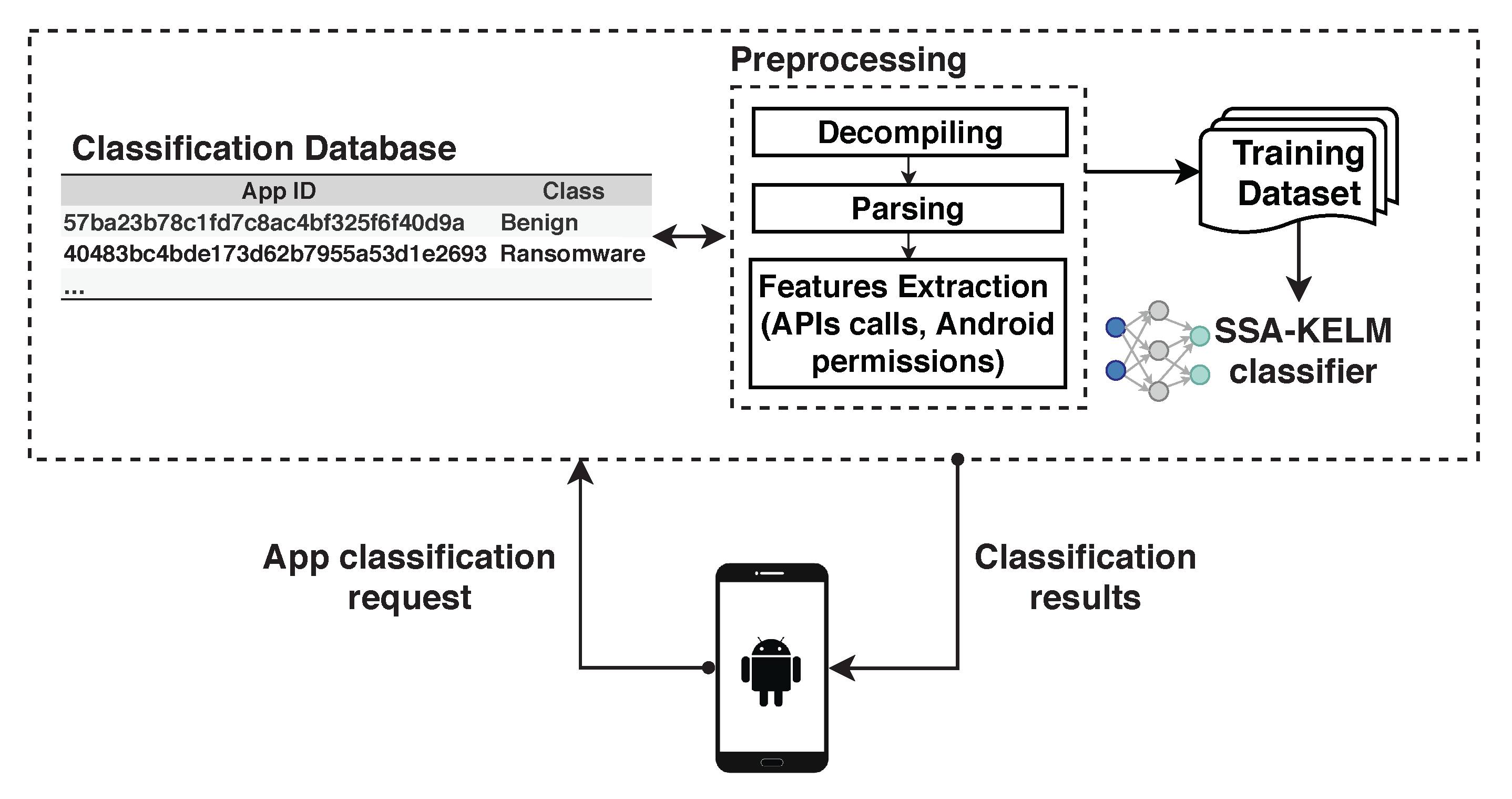
Providing ransomware detection service to Android devices is one of the main stages of the overall ransomware detection system. However, this research focuses on building an efficient predictive model to detect ransomware apps with high accuracy. Building the predictive model is a core component of any ransomware detection system. In this work, building a smart predictive model (SSA-KELM) will be executed over the cloud, not on the local Android devices. Only the app info (such as the application’s hash) will be sent from the mobile to the Ransomware detection system in order to classify the respective app as benign or ransomware. In case the app was tested before by our detection system, then its classification result will be found and sent immediately to the Android device. But if this is the first time this app is tested, then it will be decompiled and parsed to extract its features and pass them to the proposed classifier which is the role of our proposal in this paper. The result of detection will be sent to the Android device and at the same time will be logged in the system’s classification database for future use by other users’ requests. Therefore, the detection service will be lightweight as it is only called by the Android mobile devices as shown in Figure 3.
4.2. Datasets Description and Preparation
Primarily, the constructed dataset encompasses features of the application permissions and API calls that were obtained by a reverse engineering procedure. Executable mobile applications come in the Android package kit () extended file, which is a package file that is used by end-users to install mobile applications on the Android operating system. Mainly, it contains all the needed files during development including classes, resources, assets, certificates, libraries, and the manifest file. Two essential types of files are needed to extract the features of permissions and the API calls; which are the (AndroidManifest.xml) and (“.smali”) files. The (AndroidManifest.xml) file is a fundamental file that consists of all the permissions that were used by the corresponding application. Whereas, the (“.smali”) files acquired by disassembling (baksmaling) the binary executable files (“.dex”). The Apktool software is a tool that automates the process of unpacking the APK files and attains the manifest and Smali files [41].
The creation of the dataset was performed by collecting 1000 () files from benign and ransomware mobile applications. The benign applications were downloaded from the Google Play store, whereas, the ransomware apps were collected from HelDroid project, RansomProper project, Virus Total, and Koodous tools [14,20,42,43]. In order to unpack the AndroidManifest files and Smali files from all used applications; the Apktool (version = 2.3.1) was employed. Afterward, regarding the permissions features, the extracted files were scanned to report the presence of 131 types of permissions. The objective of the Android permissions is to inform the user and to have an acceptance to use sensitive data from the user’s mobile or access some system features (such as the camera). Typically, by default, the applications do not have permission to execute actions that might have a negative effect on the user, the system, or the installed mobile applications. Such permissions prevent the applications from accessing a user’s emails, keeping the device awake, or writing on the files of other applications. All the permissions which are (131) were scanned from the thousand AndroidManifest files and documented for further analysis. However, (16) permission features were removed from the original dataset since they are not used by the benign or ransomware classes.
Regarding the features from the API calls, they were considered from the Oreo Android release (Android API 27), which contains (199) API packages. All the respective applications were decompiled using the Apktool and the files with (“.smali”) extension were extracted. The “.smali” files were scanned to find the occurrences rate of API calls from both benign and ransomware applications; hence to be handled as distinguishing features. For instance, examples of used features of the API calls are Android Animation and Android Content. In consequence, the total dataset accounts for (1000) applications; where (500) are benign and (500) are ransomware. The total number of features is (314) of both the permissions and the API calls.
Frequency analysis is performed on the extracted features to indicate the occurrences of features with regard to the benign and ransomware classes, Figure 4 shows the frequency of permission features in benign and ransomware applications, where the features with a frequency less than or equal to 2% were eliminated. Obviously, the top four features observed by benign applications were the access_network_state, Internet, wake_lock, and write_external_storage, even that they were highly witnessed by the ransomware apps, too. On the other hand, the receive_boot_completed, and the read_phone_state were considerably occurred by the ransomware applications. Nonetheless, the figure shows (6) features used slightly just by the benign apps, while (12) features used only by the ransomware.
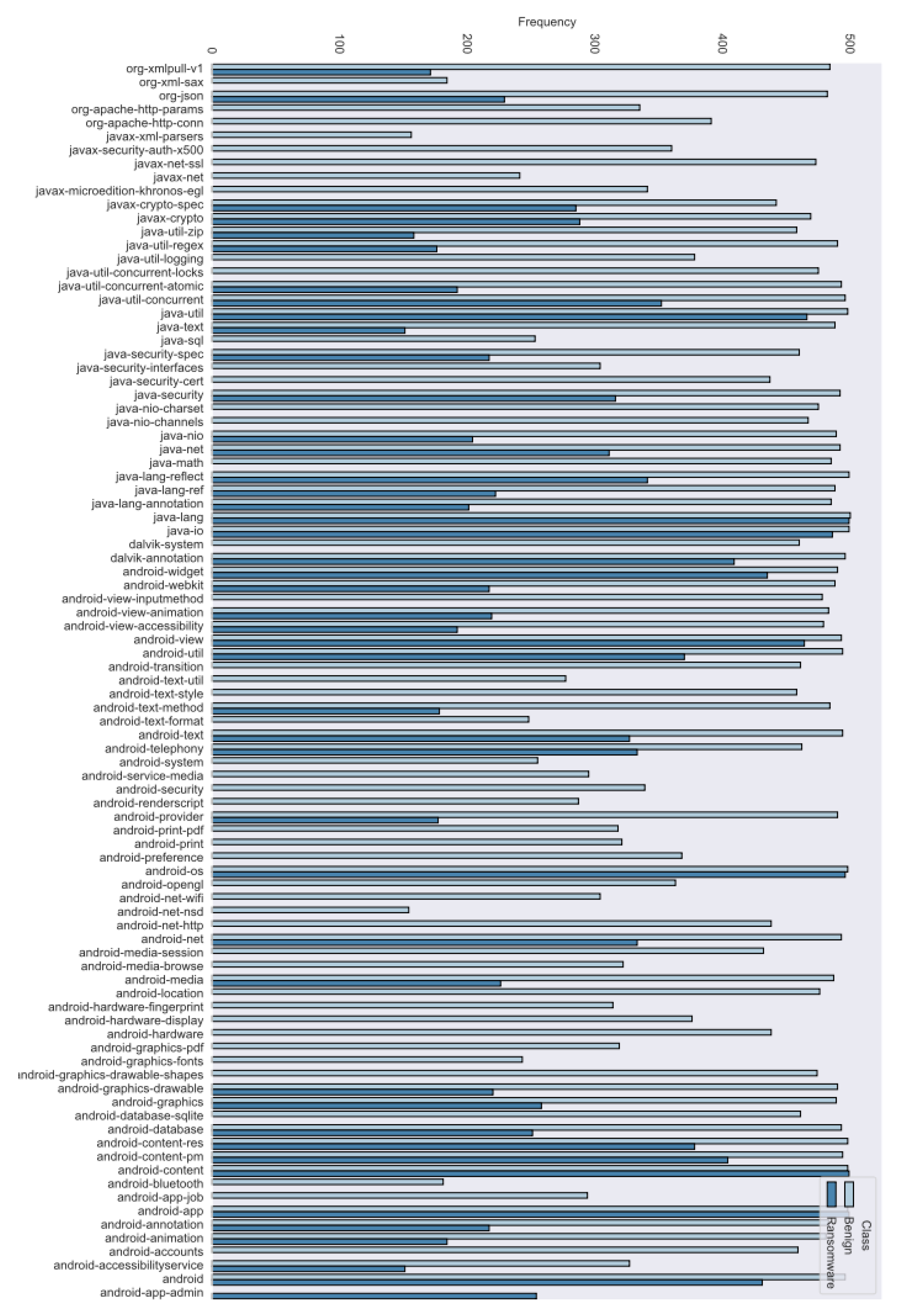
Figure 5 presents the frequency of the API features in benign and ransomware applications. In which, the features with frequency less than or equal to 30% were removed. Notably, android-app, android-content, android-os, java-io, and java-lang were the most frequent features in ransomware apps.
4.3. SSA-KELM Classifier
4.3.1. Design Issues
In this subsection, three main issues related to the design of the proposed SSA-KELM are discussed, which are the representation of the salps (solutions), the fitness function, and the binarization mechanism.
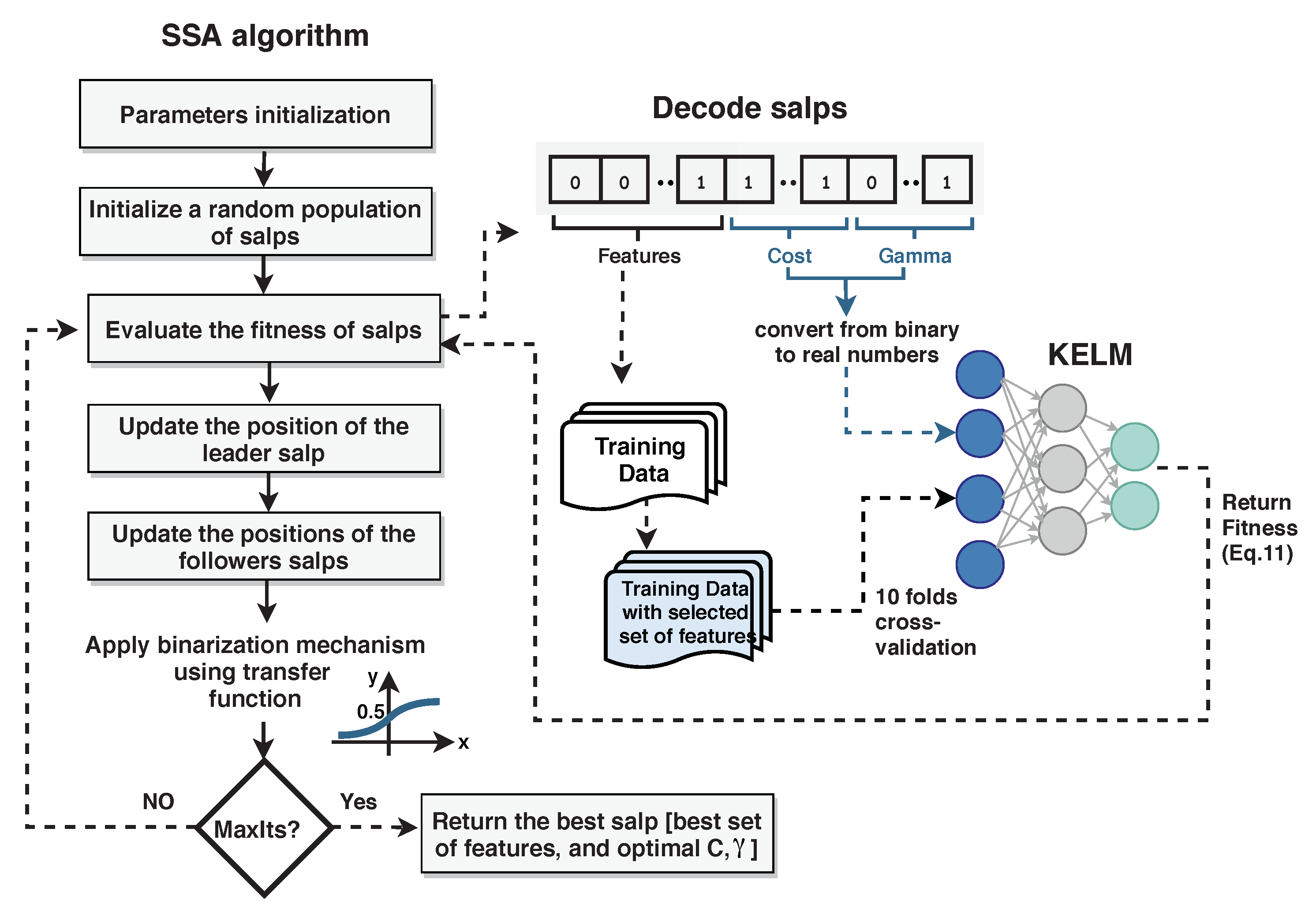
- Salp representation: each salp chain is represented as a binary vector. The length of this vector is elements, where d is the number of features in the training data. The 16 additional elements are used to encode the values of the hyperparameters of the KELM; C and , where 8 elements are used for each hyperparameter. Five elements are allocated for the whole number part and three elements are allocated for the fractional part. Figure 6 depicts an example of a salp’s vector.Figure 6. A vector representation of an individual salp that encompasses the features of the dataset, the hyperparameters of the KELM algorithm (C, ). (n) is the total number of features, () represent the digits of the cost value, and () are the digits of the value.Figure 6. A vector representation of an individual salp that encompasses the features of the dataset, the hyperparameters of the KELM algorithm (C, ). (n) is the total number of features, () represent the digits of the cost value, and () are the digits of the value.
![Applsci 10 03706 g006]()
- Fitness function: to evaluate the effectiveness of the salps, the elements of each salp are decoded as described previously and a KELM algorithm is built based on the selected features and the values of the hyperparameters obtained by the decoding process. The resulted KELM is trained on the training folds from the training dataset, then the accuracy rate which is the ratio of the correctly classified instances to the total number of instances in the training data is calculated. The accuracy rate is combined with the number of the selected features as shown in Equation (12) and returned to main procedure of the SSA as the fitness of the salp. in Equation (12) is the selected number of features, while F is the total number of features.
- Binarization mechanism: In the proposed approach, we utilize a sigmoidal s-shaped function to covert the SSA to a binary optimization algorithm. The s-shaped function is one of the most successful variants of transfer functions used in the literature in binary optimization algorithms [44]. The conversion process by the transfer functions is based on the probability assigned by them for each element in the solution vector. When the probability is greater than one, the element is rounded to 1, and vice versa as given in Equation (13). This process was first described by Kennedy and Eberhart [45] to convert the classical Particle Swarm Optimization to a binary optimizer.where is the element in x solution in the dimension, and t is the current iteration.

4.3.2. Procedure
The main procedure of the SSA-KELM can be summarized in the following steps:
- Initialize a random swarm of N binary salps.
- Evaluate the fitness of each salp as described in the previous subsection by relying on the fitness achieved by the KELM.
- Modify the position of the leading salp as in Equation (2).
- Modify the position of the followers as in Equation (4).
- Guarantee that all salps located inside the search space specified by the upper and lower bounds.
- Return to step (2) if the termination criterion is not satisfied. Otherwise, return the best solution that encompasses the optimal subset of features and the best hyperparameters values.
Figure 7 describes the steps of the proposed approach.
4.4. Model Evaluation Metrics
Algorithm evaluation is a significant aspect of developing a successful classification model. Relying on one evaluation criterion might indicate a very good model, while in terms of another, it might reflect a deterioration in the algorithm performance capability. Typically, to properly measure the performance of the algorithms in handling the variable characteristics of the data, and for a fair comparison, as well; several evaluation metrics were considered.
Herein, assessing the algorithm’s ability in distinguishing between benign data or malware, generally, depends on a set of metrics derived from the confusion matrix. The confusion matrix reveals the potential of the algorithm in truly classifying the data with respect to its actual labels. It is expressed by four types of counts (given a binary classification problem); the true positive (TP), the true negative (TN), the false positive (FP), and the false negative (FN), as represented by Table 1. Therefore, this paper incorporates the accuracy, recall, false positive rate, specificity, precision, g-mean, and the area under the curve (AUC) for measuring the performance of the proposed algorithms. Mainly, those metrics are defined as follows by considering that the positive class is the class of interest, which is the Ransomware class.
The accuracy is the ratio of the total number of classifications that were correctly labeled, it is shown by Equation (15).
Recall expresses the true positive rate, and formulated by the percentage of the relevant instances that have been identified over the total number of relevant instances. It is presented by Equation (16)
False positive rate (FPR) also known as the false alarm rate, which is the ratio of classifying the benign instances as ransomware instances (Equation (17)).
True negative rate (TNR) or the specificity, it exhibits the strength of the classifier in distinguishing the negatively classified instances of data (benign) from the positively labeled (ransomware) instances. The TNR is defined as in (Equation (18)).
Precision is the proportion of the relevant data instances over the retrieved instances. It is mathematical description is given by Equation (19).
The geometric mean (G-mean) represents the mean of the recalls in case of the multiple classes, or the mean of the recall and specificity in case of the of binary classification, it is defined by Equation (20).
The area under the curve (AUC) is defined as the area under the receiver operating characteristic (ROC) curve. AUC is deemed as a metric for evaluating the ability of the classifier in discriminating between the respective classes. Thereby, obtaining a high value of AUC is an indication of the power of the model in differentiating between the ransomware and the benign classes. Whereas, in the case of low AUC value that is approaching (0,) it means that the classifier identifies the benign data as ransomware, and counterintuitively, the ransomware as benign. The AUC is described by Equation (21).
5. Experiments and Results
The performed experiments consist mainly of two parts; analysis of the influence of leaders’ salps percentage, and the analysis of the SSA’s swarm size. Thereby, the best SSA variant with the KELM was employed for the ransomware detection and compared with conventional machine learning algorithms. In addition, a feature importance analysis has been applied to reinforce the distinguishing features of the ransomware applications. The best-obtained results in subsequent sections are marked with a bold typeface.
5.1. Experiments Setup
This sub-section presents the environmental and experimental settings for all conducted experiments. Where they were implemented using the Matlab R2016b platform over Windows server 2012. In which, the random-access memory (RAM) is 64 GB, the processor is Intel(R) Xeon(R) CPU E5-2609 v4, while the speed of the two processors is 1.70 GHz.
Initially, the proposed approach is evaluated using 10 folds cross-validation. Since the adopted SSA algorithm is used as wrapper-based feature selection; it used the KELM as a learning algorithm where its hyperparameters (C and ) were optimized using SSA. The KELM is responsible for assessing the fitness of solutions; therefore, it returns the weighted-sum of (1-accuracy) and the ratio of features, as given by Equation (12).
The SSA algorithm is a stochastic swarm-based algorithm as mentioned before; hence, diminishing the randomness effect of the algorithm requires executing it multiple times. Herein, (10) independent runs were performed with the maximum number of iterations is 50. In essence, the population size and the number of leaders are controlling parameters of the SSA that play a vital role in escalating the performance of the algorithm or degrade it if not set properly. The following subsections present a sensitivity analysis for selecting the best values of the leaders’ ratio and the population size.
5.2. Effect of Leaders Ratio
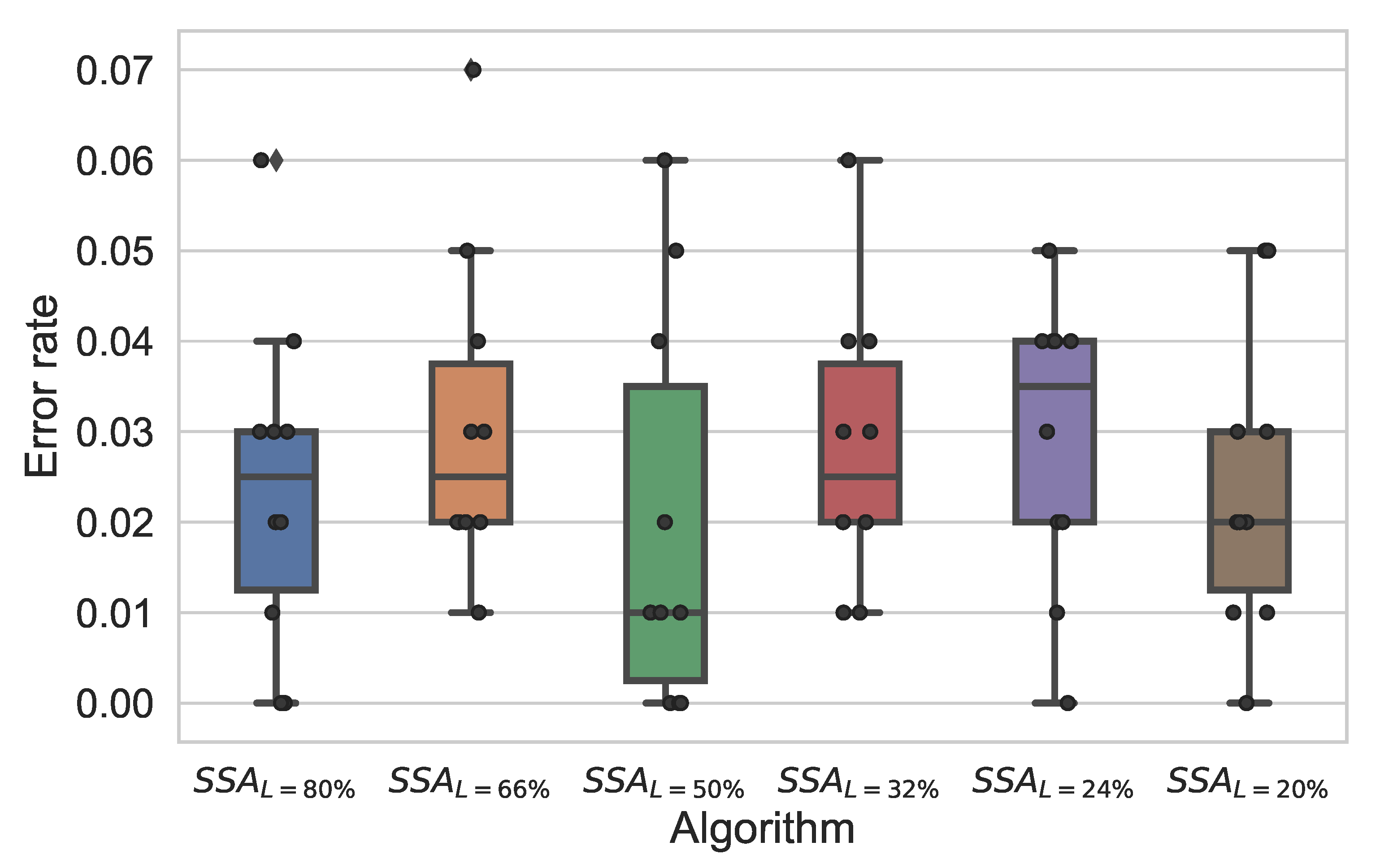
In this experiment, we study the effect of the ratio of the number of leaders to the swarm size on the performance of the proposed SSA-KELM. Table 2 and Table 3 show the evaluation results of the SSA-KELM at different ratios of leaders. From the results, it can be seen that the best results in terms of most evaluation measures are obtained at a ratio of 50%. Remarkably, it can be noticed that all ratios achieved approximately a high reduction rate which is around (44%), while the difference between the reduction rates is slight. For instance, when the leaders’ ratio is (20%), the algorithm obtained the maximal reduction rate of 49%, where the number of features was 160 out of 314. However, there is no obvious relation between the reduction rate and the number of leaders; this is demonstrated at the ratio (80%) where the reduction rate was 44.8%. In contrast, at leaders’ ratio (50%), even that the algorithm achieved the minimal reduction rate, but it markedly exhibited the best performance as it is shown by Table 3.
In this table, average accuracy, recall, FPR, TNR, Precision, G-mean, and AUC were reported at different ratios of leaders. At 50% of leaders’ ratio, the SSA performed the best results and gained superior results in terms of accuracy, TNR, precision, g-mean, and AUC, which was (98%), which is reinforced by reasonable standard deviation values. Additionally, in regards to the FPR, accomplished the minimal false positive rate (0.020), whereas at the other ratios from the highest to the lowest, they were 0.032, 0.032, 0.034, 0.024, and 0.028, respectively. Notably, regarding the recall, at all ratios, the recall was relatively close, while ratio (80%) achieved the highest recall value (98.4%). Overall, the SSA algorithm performed the best in terms of all evaluation metrics when the proportion of leaders was half the swarm. As the number of leaders has tested next is to study the influence of the SSA population size.
Figure 8 shows a box plot presentation of the error rate of the SSA algorithm at the six different ratios of leaders. Obviously, when the ratio (L) is 50%, the algorithm obtained the minimal error rate.
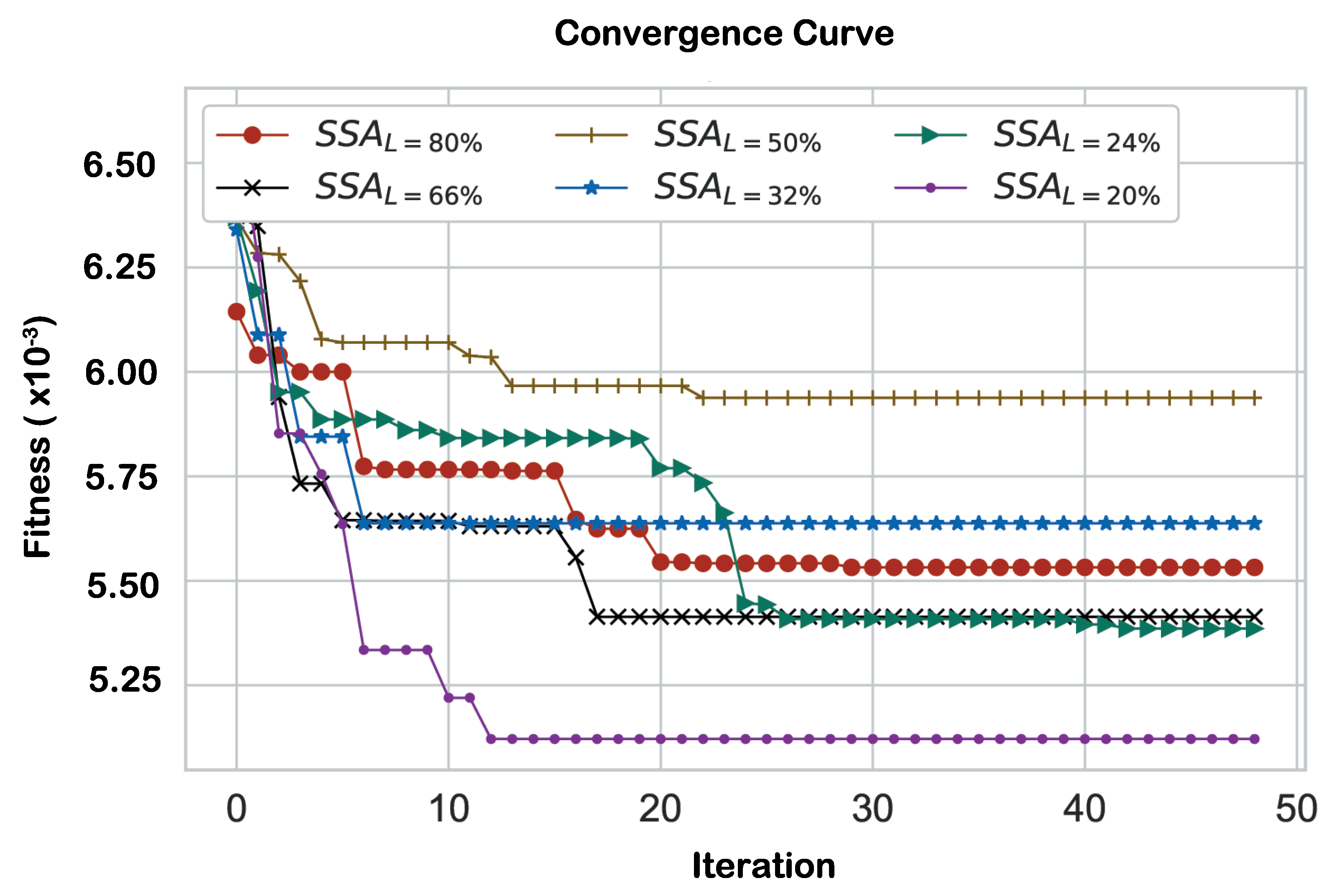
In terms of the convergence rate, Figure 9 presents the convergence plot by depicting the obtained fitness value of the SSA algorithm at each iteration of the algorithm and at six ratios of the leaders. In which, the y-axis is the fitness, and the x-axis is the iterations. It is clear from the plot that when (L=20%), the algorithm experiences a premature convergence rate, that converges very fast to the best fitness value at the eleventh iteration and then remains constant over the rest of iterations. Whereas, the other variants of leaders’ ratios exhibited different trends of convergence over the course of iterations reaching relatively optimal minimal fitness values.
5.3. Effect of Swarm Size
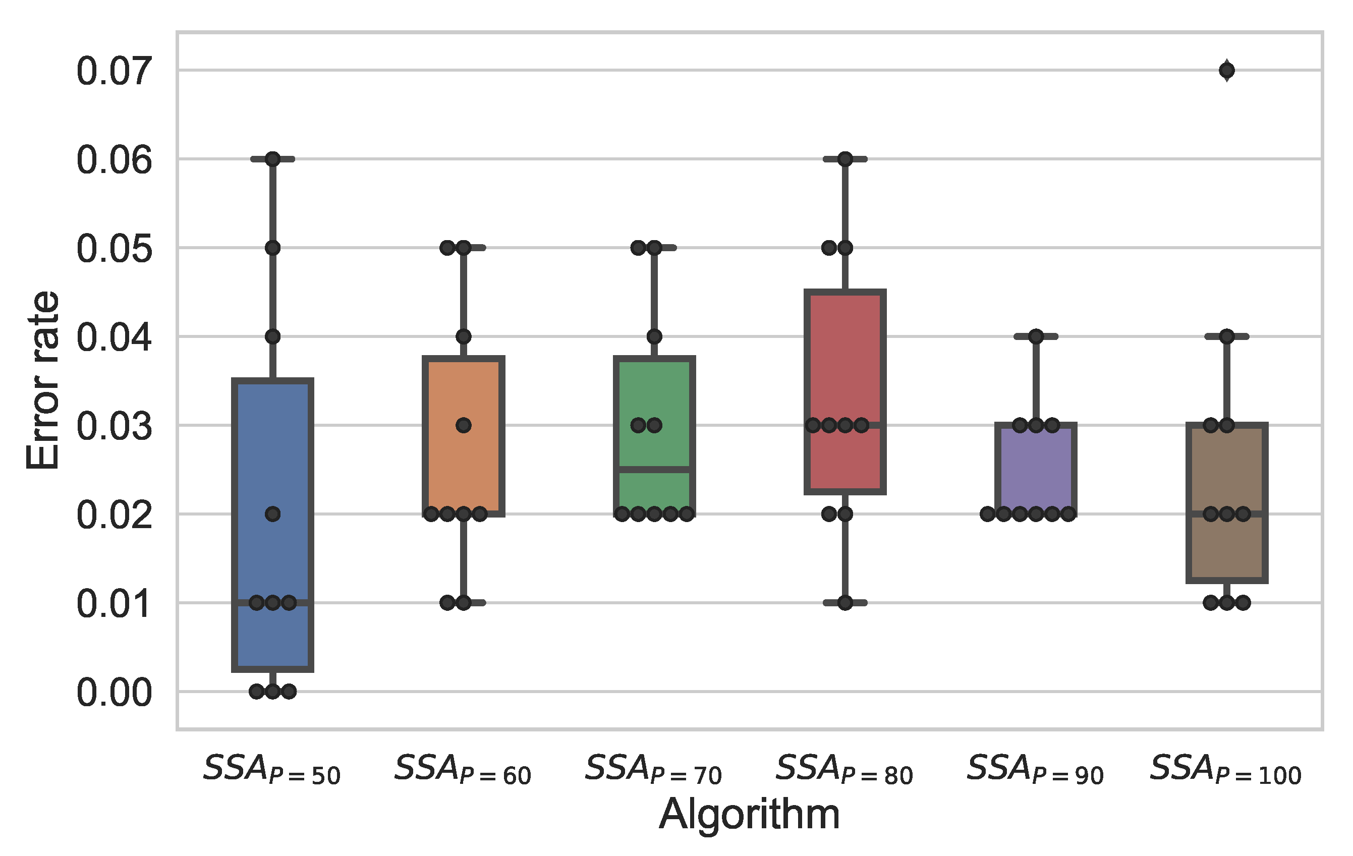
It has been long argued that population-based metaheuristic algorithms can achieve reasonable good results compared to other search algorithms if they have a good-enough large population size with enough time. However, the swarm or the population size parameter has a considerable influence on the performance of evolutionary algorithms whether in promoting or degrading it. This experiment is conducted to study and substantiate the effect of the swarm size on the performance of the proposed SSA-KELM. Hence, the swarm size of the SSA has been investigated at different values; 50, 60, 70, 80, 90, and 100, as discussed in Table 4 and Table 5. Table 4 illustrates the effect of the population size on the features reduction rate. It is clear from the table that increasing the population size not necessarily results in a better reduction rate. To illustrate, when the population size is 50, the obtained average number of features was 220.3 which yields nearly a 30% reduction in the features. However, at the swarm size of 100, it is obvious that the number of features dramatically decreased with the best-accomplished reduction rate that is 52%. On the other hand, when the swarm size was 60, 70, 80, and 90, the average number of features was higher than what is obtained by the swarm size of 100. For example, at the swarm size of (80), the average number of features was 172.3 and the reduction rate was 49.5%. Even that at all experimented swarm sizes, the SSA algorithm has decreased the number of features relatively efficiently that justified with a prominent performance results as represented by Table 5.
Table 5 compares the average performance of the SSA algorithm at different population sizes regarding the accuracy, recall, FPR, TNR, precision, g-mean, and AUC with the average standard deviation values. It is obvious from the table that the superior performance obtained when the swarm size was 50. At which, the accuracy, TNR, precision, g-mean, and AUC were 98%, while the FPR was the minimal that accounted for 0.020 with standard deviation (0.028). Examining the accuracy results, when the swarm size is greater than 50, the algorithms achieved high results with the slight difference among all, where they accomplished 97.3%, 97.0%, 96.7%, 97.5%, and 97.4%, in ascending order. Regarding the recall, even that the SSA algorithm at the size (50) achieved 98%, but at sizes (90, 100) the SSA algorithm could perform 98.2%, while in contrast, the SSA at (90, 100) performed worst in terms of FPR. For instance, when the size=90, the FPR=0.032, and when it was 100, the FPR=0.034, however, at 50, the FPR=0.020. Nonetheless, regarding the TNR, the SSA at (50, 60, 70, 80, 90, and 100) achieved 98%, 96.8%, 97%, 96%, 96.8%, and 96.6%, respectively. Similarly, at the precision, at 50, the algorithm achieved the best (98%), whereas, at 80, it achieved the minimal precision (96.1%). Additionally, at both g-mean and AUC, the best performance attained at swarm size of (50) with a performance of (98%) and with feasible standard deviation, however, (80) achieved the minimum, which is (96.7%). To sum up, the SSA algorithm accomplished striking results with a considerable feature reduction ratio. To support the superiority of the proposed SSA-KELM, it has been compared with well-known classical machine learning algorithms as given by the following sub-section.
Figure 10 describes the error rate at various swarm sizes of SSA. Markedly, when the swarm size (P) is 50, the outperformed the other variants and attained the best error rate results, while when (P = 80), the algorithm performed the worst performance regarding the error rate.
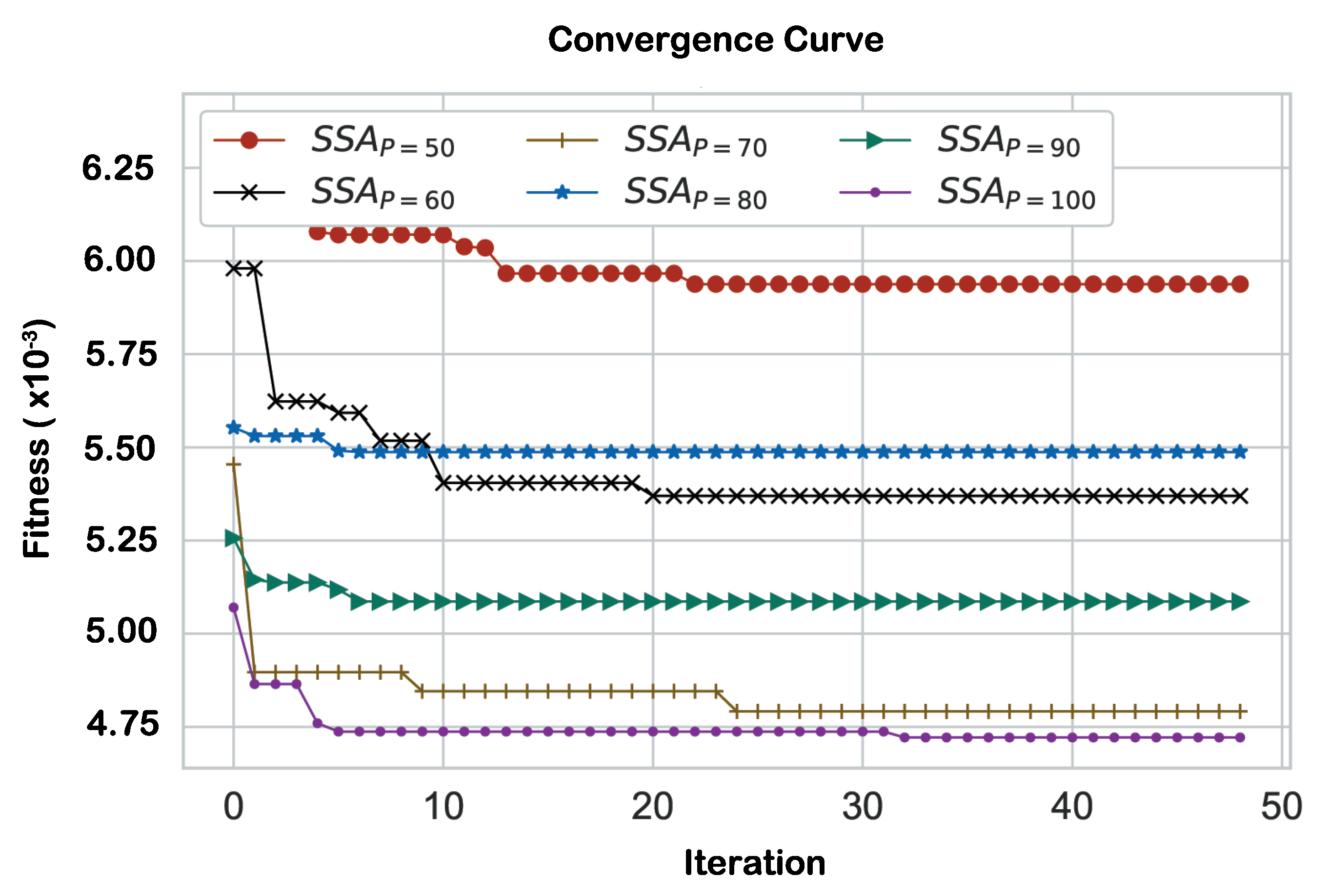
Nonetheless, Figure 11 shows the convergence plots of the SSA algorithm at various population sizes. It can be noticed that at all the experimented population sizes, the SSA algorithm exhibits similar, good convergence rates that eventually could reach such best fitness values. For instance, at iteration (22), it reached a minimal fitness of (0.00059), while at , the algorithm optimally minimized the fitness to (0.00045). Generally speaking, the SSA algorithm has a successful convergence trend toward optimal solutions over the course of iterations with slight difference in relation to the population size effect.
5.4. Sensitivity Analysis of Fitness Parameters
Table 6 presents a sensitivity analysis of the () parameter of the fitness function of the SSA algorithm. In Equation (12), the fitness constitutes a weighted-sum of the accuracy and the ratio of the selected subset of features. The weighted-sum approach is a classical methodology to handle a multi-objective optimization problem as a single-objective problem. Where the aim is to optimize the weighted-sum of the utilized objectives. Herein, two objectives were considered; the accuracy, and the ratio of the selected features. In which, the accuracy is weighted by the () parameter, and the ratio of selected features was weighted by the multiplier (1-). The coefficient () has a controlling behavior for selecting the optimal salp solution, which quantifies the importance of the corresponding objectives. However, there is no guarantee that the randomly chosen value of () will produce the optimal solution; therefore, tuning the () parameter is imperative.
Table 6 shows performance of the SSA algorithm at five different values of (), where it belongs to . It is clear from the table that when , it obtained the best results in terms of accuracy, recall, TNR, precision, g-mean, and AUC, which all attained (98.0%). The minimal FPR value was obtained at a percentage of (2%). Although, when , the algorithm could achieve drastically better performance. In contrast, in terms of the reduction rate of features, when equals 0.2, the algorithm achieved extremely better. So, the best reduction rate is obtained when () with percentage of 54.4%. Whereas, when (), it achieved a reduction rate of 29.9%, and 28.7%, respectively.
5.5. Comparison Results
In this subsection, the performance of the SSA-KELM is compared with the performance of a set of well-known classifiers; which are Naive Bayes (NB), Decision Tree C4.5 (J48), very powerful ensemble classifiers which are Random Forests (RF), AdaBoost, Bagging, and XGBoost. In addition, it is compared with another well-established swarm intelligence algorithm which is the particle swarm optimization (PSO). For which the inertia weight (), the constraints () are set to value (2), and the maximum velocity is (6). The hyperparameters of XGBoost are optimized using a grid search algorithm, which determines a range of values (search space) for each hyperparameter. The grid search is used to optimize a five hyperparameters of XGBoost; which are the minimum-child-weight: [2, 5, 8], gamma: [0.1, 1, 1.5], number-of-estimators: [50, 120, 323], learning-rate: [0.3, 0.5, 0.9], and the maximum-depth: [6, 10, 15]. The XGBoost-Grid is evaluated based on 10-folds cross-validation, where the best results obtained at gamma = 0.1, min-child-weight = 2, number-of-estimators = 50, learning-rate = 0.9, and the maximum-depth = 6. Mainly, all classifiers evaluated using 10-folds cross-validation and implemented using Weka workbench [46].
The results of this comparison are shown in Table 7. The evaluation results show that the SSA-KELM outperforms all the other classifiers and swarm intelligence methods regarding the majority of the measures. Although some classifiers like Bagging and AdaBoosting showed very competitive results, they used the full set of features without any reduction like in the SSA-KELM. Moreover, the SSA-KELM outperformed the PSO-KELM in terms of all evaluation measures indicating its powerful capability. Therefore, the SSA-KELM has merits over conventional machine learning classifiers, where it exhibited efficacy in performance and in minimizing the selected subset of features.
Features Importance
Feature importance analysis has a fundamental role in identifying to what extent the features play a part in the predictive power of the model. In this regard, the frequencies of selected subsets of features generated by the SSA algorithm were utilized to investigate the importance of features. In other words, as the SSA algorithm generates a new subset of features at each iteration; the frequency of the feature selection for all features is calculated over the number of iterations. Hence, the importance (FI) of a feature (i) is given by Equation (22), where L is the maximum number of iterations.
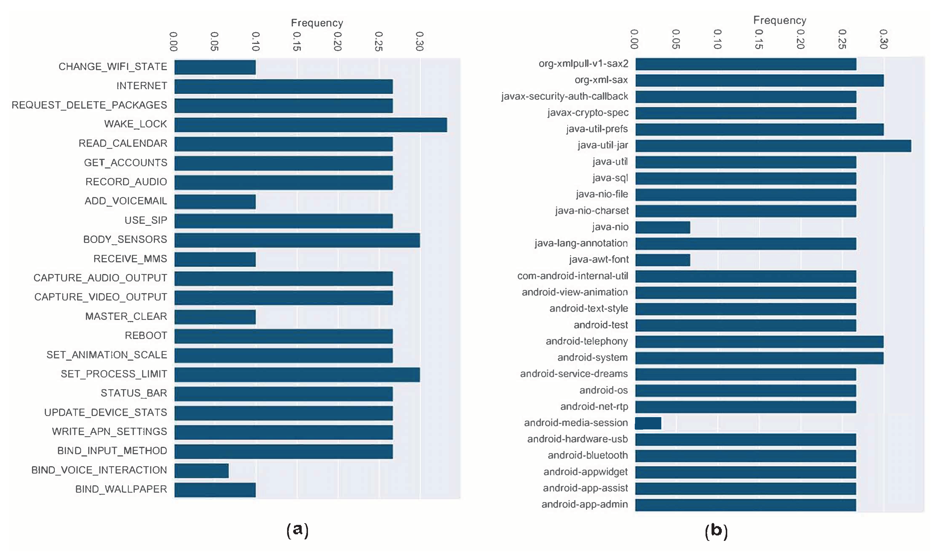
Figure 12 presents the most important features of the API calls and permissions while training the SSA-KELM at the ratio of leaders (L=50%), and swarm size (P=50). In sub-figure (a), the plot shows the most and least occurred permissions features. In which, the most important features were reported when the importance , while the least important, were reported when the importance . It is obvious from sub-figure (a) that WAKE_LOCK, BODY_SENSORS, and the SET_PROCESS_LIMIT were the most important features. These permissions allow the ransomware attackers to stop the processors and screens from sleeping, or to grant them access for collecting personal data such as the sensors’ readings. Such information could be targeted by ransomwares to be encrypted or locked as they are considered private and important. Additionally, as ransomware runs processes behind the scene, it might modify the state of the SET_PROCESS_LIMIT permission to change the maximum number of concurrently running processes. Whereas, sub-figure (b) represents the most important API features. Where org-xml-sax, java-util-prefs, java-util-jar, android-telephony, and android-system were the most contributed features to the prediction efficacy. These API calls allow the attacker to read user-related data that existed in different formats including the Extensible Markup Language (XML) format, and the Java Archive format (Zip format). Also, they allow ransomwares to monitor basic phone information including network type, connection state, and manipulating phone number strings which could be an indication of invasion [31]. Moreover, andorid.system API can grant the attackers access to low-level system functionalities, which makes them more powerful due to the ability to access the underlying primitives used to implement high-level APIs.
6. Conclusions and Future Works
In recent years, we have been witnessing the emergence of a dangerous threat attacking the computer and mobile systems, which is the ransomware. Since ransomware results in serious damage for the users’ files and system; developing a robust ransomware detection approach is imperative. A hybrid swarm-intelligent machine learning approach is proposed in this work for Android ransomware detection based on two types of features: application permissions and API packages’ calls. In the proposed hybrid approach, Salp Swarm Algorithm is utilized for optimizing the hyperparameters of Kernel Extreme Learning Machine and performing feature selection, simultaneously. The experiments based on the collected data show that the proposed model outperforms very powerful classifiers in terms of detection power. Further analysis of the selected features by the model shows that some features were much frequent than others, like WAKE_LOCK, and java-util-jar, meaning that they have higher contribution than other features for enhancing the prediction capability of the proposed approach. However, in terms of further potential work, having a larger dataset promotes the effectiveness of the learning algorithms and increases the chance of capturing more insightful characteristics of the ransomware, which elevates the algorithm detection capacity. Therefore, employing advanced machine learning such as deep learning becomes more feasible.
Author Contributions
Conceptualization; H.F. and I.M.; Methodology, H.F. and M.E.; Validation, H.F. and M.E., M.H. and I.M.; Data curation, I.M.; Writing original draft preparation, H.F., M.H., M.E. and I.M.; Writing review and editing, H.F. and I.A.; Supervision H.F.; Project administration, I.M. and H.F. All authors have read and agreed to the published version of the manuscript.
Funding
This research received no external funding. The APC is funded by Prince Sultan University.
Acknowledgments
We would like to acknowledge the Security Engineering Lab (sel.psu.edu.sa) team and Prince Sultan University for supporting this work.
Conflicts of Interest
The authors declare no conflict of interest.
References
- O’Dea, S. Number of Smartphone Users Worldwide from 2016 to 2021. Available online: www.Statista.com (accessed on 28 February 2020).
- Perlroth, N. Android Phones Hit by Ransomware. Available online: www.nytimes.com (accessed on 22 March 2020).
- Malwarebytes-Labs. All About Malware. Available online: www.malwarebytes.com (accessed on 24 March 2020).
- Herrera Silva, J.A.; Barona López, L.I.; Valdivieso Caraguay, Á.L.; Hernández-Álvarez, M. A Survey on Situational Awareness of Ransomware Attacks—Detection and Prevention Parameters. Remote Sens. 2019, 11, 1168. [Google Scholar] [CrossRef] [Green Version]
- Ameer, M. Android Ransomware Detection using Machine Learning Techniques to Mitigate Adversarial Evasion Attacks. Ph.D. Thesis, Capital University, Columbus, OH, USA, 2019. [Google Scholar]
- Blum, A.L.; Langley, P. Selection of relevant features and examples in machine learning. Artif. Intell. 1997, 97, 245–271. [Google Scholar] [CrossRef] [Green Version]
- Yang, X.S. Nature-Inspired Metaheuristic Algorithms; Luniver Press: Beckington, UK, 2010; ISBN 9781905986088. [Google Scholar]
- Al Shorman, A.; Faris, H.; Aljarah, I. Unsupervised intelligent system based on one class support vector machine and Grey Wolf optimization for IoT botnet detection. J. Ambient Intell. Humaniz. Comput. 2019, 1–17. [Google Scholar] [CrossRef]
- Messaoud, R.B. Extraction of uncertain parameters of single and double diode model of a photovoltaic panel using Salp Swarm algorithm. Measurement 2020, 154, 107446. [Google Scholar] [CrossRef]
- Abbassi, R.; Abbassi, A.; Heidari, A.A.; Mirjalili, S. An efficient salp swarm-inspired algorithm for parameters identification of photovoltaic cell models. Energy Convers. Manag. 2019, 179, 362–372. [Google Scholar] [CrossRef]
- Mirjalili, S.; Gandomi, A.H.; Mirjalili, S.Z.; Saremi, S.; Faris, H.; Mirjalili, S.M. Salp Swarm Algorithm: A bio-inspired optimizer for engineering design problems. Adv. Eng. Softw. 2017, 114, 163–191. [Google Scholar] [CrossRef]
- Hegazy, A.E.; Makhlouf, M.; El-Tawel, G.S. Feature selection using chaotic salp swarm algorithm for data classification. Arab. J. Sci. Eng. 2019, 44, 3801–3816. [Google Scholar] [CrossRef]
- Ala’M, A.Z.; Heidari, A.A.; Habib, M.; Faris, H.; Aljarah, I.; Hassonah, M.A. Salp Chain-Based Optimization of Support Vector Machines and Feature Weighting for Medical Diagnostic Information Systems. In Evolutionary Machine Learning Techniques; Springer: Berlin, Germany, 2020; pp. 11–34. [Google Scholar]
- Andronio, N.; Zanero, S.; Maggi, F. Heldroid: Dissecting and detecting mobile ransomware. In Research in Attacks, Intrusions, and Defenses, Proceedings of the 18th International Symposium on Recent Advances in Intrusion Detection, Kyoto, Japan, 2–4 November 2015; Springer: Berlin, Germany, 2015; pp. 382–404. [Google Scholar]
- Zheng, C.; Dellarocca, N.; Andronio, N.; Zanero, S.; Maggi, F. Greateatlon: Fast, static detection of mobile ransomware. In Security and Privacy in Communication Networks, Proceedings of the 12th International Conference, Security and Privacy in Communication Systems, Guangzhou, China, 10–12 October 2016; Springer: Berlin, Germany, 2016; pp. 617–636. [Google Scholar]
- Song, S.; Kim, B.; Lee, S. The effective ransomware prevention technique using process monitoring on android platform. Mob. Inf. Syst. 2016, 2016, 2946735. [Google Scholar] [CrossRef] [Green Version]
- Gharib, A.; Ghorbani, A. Dna-droid: A real-time android ransomware detection framework. In Network and System Security, Proceedings of the 11th International Conference on Network and System Security, Helsinki, Finland, 21–23 August 2017; Springer: Berlin, Germany, 2017; pp. 184–198. [Google Scholar]
- Almomani, I.; Khayer, A. Android Applications Scanning: The Guide. In Proceedings of the 2019 International Conference on Computer and Information Sciences (ICCIS), Sakaka, Saudi Arabia, 3–4 April 2019; pp. 1–5. [Google Scholar]
- Almomani, I.; Alenezi, M. Android Application Security Scanning Process. In Telecommunication Systems; Alimi, I.A., Monteiro, P.P., Teixeira, A.L., Eds.; IntechOpen: Rijeka, Croatia, 2019; Chapter 3. [Google Scholar] [CrossRef] [Green Version]
- Chen, J.; Wang, C.; Zhao, Z.; Chen, K.; Du, R.; Ahn, G.J. Uncovering the face of android ransomware: Characterization and real-time detection. IEEE Trans. Inf. Forensics Secur. 2017, 13, 1286–1300. [Google Scholar] [CrossRef]
- Canfora, G.; Mercaldo, F.; Visaggio, C.A. An hmm and structural entropy based detector for android malware: An empirical study. Comput. Secur. 2016, 61, 1–18. [Google Scholar] [CrossRef]
- Chen, S.; Xue, M.; Tang, Z.; Xu, L.; Zhu, H. Stormdroid: A streaminglized machine learning-based system for detecting android malware. In Proceedings of the 11th ACM on Asia Conference on Computer and Communications Security, Xi’an, China, 30 May–3 June 2016; pp. 377–388. [Google Scholar]
- Ahmadi, M.; Sotgiu, A.; Giacinto, G. Intelliav: Toward the feasibility of building intelligent anti-malware on android devices. In Machine Learning and Knowledge Extraction, Proceedings of the International Cross-Domain Conference for Machine Learning and Knowledge Extraction, Reggio, Italy, 29 August–1 September 2017; Springer: Berlin, Germany, 2017; pp. 137–154. [Google Scholar]
- Garcia, J.; Hammad, M.; Malek, S. Lightweight, obfuscation-resilient detection and family identification of android malware. ACM Trans. Softw. Eng. Methodol. 2018, 26, 1–29. [Google Scholar] [CrossRef]
- Cimitile, A.; Mercaldo, F.; Nardone, V.; Santone, A.; Visaggio, C.A. Talos: No more ransomware victims with formal methods. Int. J. Inf. Secur. 2018, 17, 719–738. [Google Scholar] [CrossRef]
- Su, D.; Liu, J.; Wang, X.; Wang, W. Detecting Android locker-ransomware on chinese social networks. IEEE Access 2018, 7, 20381–20393. [Google Scholar] [CrossRef]
- Sharma, G.; Johri, A.; Goel, A.; Gupta, A. Enhancing RansomwareElite App for Detection of Ransomware in Android Applications. In Proceedings of the 2018 Eleventh International Conference on Contemporary Computing (IC3), Noida, India, 2–4 August 2018; pp. 1–4. [Google Scholar]
- Poudyal, S.; Dasgupta, D.; Akhtar, Z.; Gupta, K. A multi-level ransomware detection framework using natural language processing and machine learning. In Proceedings of the 14th International Conference on Malicious and Unwanted Software (MALCON), Nantucket, MA, USA, 2–4 October 2019. [Google Scholar]
- Scalas, M.; Maiorca, D.; Mercaldo, F.; Visaggio, C.A.; Martinelli, F.; Giacinto, G. On the effectiveness of system API-related information for Android ransomware detection. Comput. Secur. 2019, 86, 168–182. [Google Scholar] [CrossRef] [Green Version]
- Alzahrani, N.; Alghazzawi, D. A Review on Android Ransomware Detection Using Deep Learning Techniques. In Proceedings of the 11th International Conference on Management of Digital EcoSystems, Limassol, Cyprus, 12–14 November 2019; pp. 330–335. [Google Scholar]
- Alsoghyer, S.; Almomani, I. Ransomware Detection System for Android Applications. Electronics 2019, 8, 868. [Google Scholar] [CrossRef] [Green Version]
- Alsoghyer, S.; Almomani, I. On the Effectiveness of Application Permissions for Android Ransomware Detection. In Proceedings of the 6th Conference on Data Science and Machine Learning Applications (CDMA), Riyadh, Saudi Arabia, 4–5 March 2020; pp. 94–99. [Google Scholar]
- Hwang, J.; Kim, J.; Lee, S.; Kim, K. Two-Stage Ransomware Detection Using Dynamic Analysis and Machine Learning Techniques. Wirel. Pers. Commun. 2020, 1–13. [Google Scholar] [CrossRef]
- Abdullah, Z.; Muhadi, F.W.; Saudi, M.M.; Hamid, I.R.A.; Foozy, C.F.M. Android Ransomware Detection Based on Dynamic Obtained Features. In Recent Advances on Soft Computing and Data Mining, Proceedings of the Fourth International Conference on Soft Computing and Data Mining, Melaka, Malaysia, 22–23 January 2020; Springer: Berlin, Germany, 2020; pp. 121–129. [Google Scholar]
- Aljarah, I.; Mafarja, M.; Heidari, A.A.; Faris, H.; Zhang, Y.; Mirjalili, S. Asynchronous accelerating multi-leader salp chains for feature selection. Appl. Soft Comput. 2018, 71, 964–979. [Google Scholar] [CrossRef]
- Faris, H.; Mafarja, M.M.; Heidari, A.A.; Aljarah, I.; Ala’M, A.Z.; Mirjalili, S.; Fujita, H. An efficient binary salp swarm algorithm with crossover scheme for feature selection problems. Knowl. Based Syst. 2018, 154, 43–67. [Google Scholar] [CrossRef]
- Ahmed, S.; Mafarja, M.; Faris, H.; Aljarah, I. Feature selection using salp swarm algorithm with chaos. In Proceedings of the 2nd International Conference on Intelligent Systems, Metaheuristics & Swarm Intelligence—ACM, Phuket, Thailand, 24–25 March 2018; pp. 65–69. [Google Scholar]
- Zhang, J.; Wang, Z.; Luo, X. Parameter estimation for soil water retention curve using the salp swarm algorithm. Water 2018, 10, 815. [Google Scholar] [CrossRef] [Green Version]
- Huang, G.B.; Zhou, H.; Ding, X.; Zhang, R. Extreme learning machine for regression and multiclass classification. IEEE Trans. Syst. Man Cybern. Part B Cybern. 2012, 42, 513–529. [Google Scholar] [CrossRef] [Green Version]
- Huang, G.B.; Zhu, Q.Y.; Siew, C.K. Extreme learning machine: A new learning scheme of feedforward neural networks. In Proceedings of the IEEE international joint conference on neural networks (IEEE Cat. No. 04CH37541), Budapest, Hungary, 25–29 July 2004; Volume 2, pp. 985–990. [Google Scholar]
- Winsniewski, R. Android–Apktool: A Tool for Reverse Engineering Android Apk Files. 2012. Available online: http://ibotpeaches.github.io/Apktool/ (accessed on 26 May 2020).
- VirusTotal Malware Intelligence Services. (n.d.). Retrieved April 2020. Available online: https://www.virustotal.com/learn/ (accessed on 20 March 2020).
- Koodous. Retrieved April 2020. Available online: https://koodous.com/ (accessed on 20 March 2020).
- Mirjalili, S.; Lewis, A. S-shaped versus V-shaped transfer functions for binary particle swarm optimization. Swarm Evol. Comput. 2013, 9, 1–14. [Google Scholar] [CrossRef]
- Kennedy, J.; Eberhart, R.C. A discrete binary version of the particle swarm algorithm. In Proceedings of the IEEE International Conference on Systems, Man, and Cybernetics. Computational Cybernetics and Simulation, Orlando, FL, USA, 12–15 October 1997; Volume 5, pp. 4104–4108. [Google Scholar]
- Hall, M.; Frank, E.; Holmes, G.; Pfahringer, B.; Reutemann, P.; Witten, I.H. The WEKA data mining software: An update. ACM SIGKDD Explor. Newsl. 2009, 11, 10–18. [Google Scholar] [CrossRef]
Figure 1.
A representation of the SSA algorithm, which shows the leader and follower salps.

Figure 2.
A structural representation of the KELM algorithm.

Figure 3.
An illustration of an intelligent Android ransomware detection system.

Figure 4.
A bar chart depicts the permission features occurrences in the benign and ransomware classes. The features with less than 2% occurrences were discarded.
Figure 4.
A bar chart depicts the permission features occurrences in the benign and ransomware classes. The features with less than 2% occurrences were discarded.

Figure 5.
A bar chart shows the API features occurrences in the benign and ransomware classes. The features with less than 30% occurrences were discarded.
Figure 5.
A bar chart shows the API features occurrences in the benign and ransomware classes. The features with less than 30% occurrences were discarded.

Figure 7.
A structural representation of the methodology flow that describes the process of searching for the optimal set of features and the best hyperparameters.
Figure 7.
A structural representation of the methodology flow that describes the process of searching for the optimal set of features and the best hyperparameters.

Figure 8.
Box plots presentation of the SSA algorithm at different ratios of leaders.

Figure 9.
Convergence curves of the SSA algorithm at different ratios of leaders.

Figure 10.
Box plots presentation of the SSA algorithm at different population sizes.

Figure 11.
Convergence curves of the SSA algorithm at different population sizes.

Figure 12.
A representation of the most important features at . The reported features are attained when the importance (>0.25) and (<0.10). Sub-figure (a) shows the importance of the permission features, while sub-figure (b) depicts the importance of the API features.
Figure 12.
A representation of the most important features at . The reported features are attained when the importance (>0.25) and (<0.10). Sub-figure (a) shows the importance of the permission features, while sub-figure (b) depicts the importance of the API features.


Table 1.
Confusion matrix.
| Actual | ||
|---|---|---|
| Ransomware | Benign | |
| Predicted Ransomware | TP | FP |
| Predicted Benign | FN | TN |
Table 2.
The effect of the ratio of leaders on the reduction rate and the average number of selected features.
Table 2.
The effect of the ratio of leaders on the reduction rate and the average number of selected features.
| Ratio of Leaders | Number of Leaders | Reduction Rate | Average No. of Features |
|---|---|---|---|
| 80% | 40 | 44.8% | 173.3 |
| 66% | 33 | 45.2% | 177.2 |
| 50% | 25 | 29.9% | 220.3 |
| 32% | 16 | 45.8% | 170.1 |
| 24% | 12 | 46.4% | 168.2 |
| 20% | 10 | 49.0% | 160.0 |
Table 3.
The performance evaluation of the SSA algorithm at different ratios of leaders, in terms of average accuracy, recall, FPR, TNR, precision, g-mean, and AUC.
Table 3.
The performance evaluation of the SSA algorithm at different ratios of leaders, in terms of average accuracy, recall, FPR, TNR, precision, g-mean, and AUC.
| Ratio of Leaders | Accuracy | Recall | FPR | TNR | Precision | G-mean | AUC |
|---|---|---|---|---|---|---|---|
| avg ± std | avg ± std | avg ± std | avg ± std | avg ± std | avg ± std | avg ± std | |
| 80 % | 0.976 ± 0.018 | 0.984± 0.021 | 0.032 ± 0.023 | 0.968 ± 0.023 | 0.969 ± 0.023 | 0.976 ± 0.018 | 0.976 ± 0.018 |
| 66 % | 0.969 ± 0.018 | 0.970 ± 0.019 | 0.032 ± 0.036 | 0.968 ± 0.036 | 0.969 ± 0.032 | 0.969 ± 0.018 | 0.969 ± 0.018 |
| 50 % | 0.980± 0.022 | 0.980 ± 0.021 | 0.020± 0.028 | 0.980± 0.028 | 0.980± 0.027 | 0.980± 0.022 | 0.980± 0.022 |
| 32 % | 0.972 ± 0.015 | 0.978 ± 0.018 | 0.034 ± 0.025 | 0.966 ± 0.025 | 0.967 ± 0.024 | 0.972 ± 0.016 | 0.972 ± 0.015 |
| 24 % | 0.971 ± 0.016 | 0.966 ± 0.025 | 0.024 ± 0.021 | 0.976 ± 0.021 | 0.976 ± 0.020 | 0.971 ± 0.016 | 0.971 ± 0.016 |
| 20 % | 0.976 ± 0.016 | 0.980 ± 0.016 | 0.028 ± 0.029 | 0.972 ± 0.029 | 0.973 ± 0.027 | 0.976 ± 0.017 | 0.976 ± 0.016 |
Table 4.
The influence of several population sizes of the SSA algorithm in terms of reduction rate and average number of features.
Table 4.
The influence of several population sizes of the SSA algorithm in terms of reduction rate and average number of features.
| Population Size | Reduction Rate | Average No. of Features |
|---|---|---|
| 50 | 29.9% | 220.3 |
| 60 | 46.7% | 167.3 |
| 70 | 51.0% | 153.8 |
| 80 | 45.1% | 172.3 |
| 90 | 49.5% | 158.7 |
| 100 | 52.0% | 150.7 |
Table 5.
The performance evaluation of the SSA at (50%) of the ratio of leaders at different population sizes, in terms of average accuracy, recall, FPR, TNR, precision, g-mean, and AUC.
Table 5.
The performance evaluation of the SSA at (50%) of the ratio of leaders at different population sizes, in terms of average accuracy, recall, FPR, TNR, precision, g-mean, and AUC.
| Population Size | Accuracy | Recall | FPR | TNR | Precision | G-Mean | AUC |
|---|---|---|---|---|---|---|---|
| avg ± std | avg ± std | avg ± std | avg ± std | avg ± std | avg ± std | avg ± std | |
| 50 | 0.980± 0.022 | 0.980 ± 0.021 | 0.020± 0.028 | 0.980± 0.028 | 0.980± 0.027 | 0.980± 0.022 | 0.980± 0.022 |
| 60 | 0.973 ± 0.015 | 0.978 ± 0.018 | 0.032 ± 0.027 | 0.968 ± 0.027 | 0.969 ± 0.026 | 0.973 ± 0.015 | 0.973 ± 0.015 |
| 70 | 0.970 ± 0.012 | 0.970 ± 0.014 | 0.030 ± 0.030 | 0.970 ± 0.030 | 0.971 ± 0.029 | 0.970 ± 0.013 | 0.970 ± 0.012 |
| 80 | 0.967 ± 0.016 | 0.974 ± 0.019 | 0.040 ± 0.016 | 0.960 ± 0.016 | 0.961 ± 0.016 | 0.967 ± 0.016 | 0.967 ± 0.016 |
| 90 | 0.975 ± 0.007 | 0.982 ± 0.022 | 0.032 ± 0.010 | 0.968 ± 0.010 | 0.969 ± 0.009 | 0.975 ± 0.007 | 0.975 ± 0.007 |
| 100 | 0.974 ± 0.018 | 0.982 ± 0.018 | 0.034 ± 0.034 | 0.966 ± 0.034 | 0.968 ± 0.032 | 0.974 ± 0.019 | 0.974 ± 0.018 |
Table 6.
The effect of alpha parameter on the fitness of the SSA algorithm.
| Evaluation Metrics | α | ||||
|---|---|---|---|---|---|
| 0.001 | 0.01 | 0.05 | 0.1 | 0.2 | |
| Accuracy | 0.980 | 0.972 | 0.972 | 0.971 | 0.970 |
| Recall | 0.980 | 0.980 | 0.974 | 0.980 | 0.980 |
| FPR | 0.020 | 0.036 | 0.030 | 0.038 | 0.040 |
| TNR | 0.980 | 0.964 | 0.970 | 0.962 | 0.960 |
| Precision | 0.980 | 0.965 | 0.970 | 0.963 | 0.962 |
| G-mean | 0.980 | 0.972 | 0.972 | 0.971 | 0.970 |
| AUC | 0.980 | 0.972 | 0.972 | 0.971 | 0.970 |
| Average No. of features | 220.3 | 224 | 154.9 | 154.9 | 143.1 |
| Reduction rate | 29.9% | 28.7% | 50.7% | 50.7% | 54.4% |
Table 7.
Comparison of the performance of the SSA-KELM with conventional machine learning algorithms in terms of various evaluation metrics.
Table 7.
Comparison of the performance of the SSA-KELM with conventional machine learning algorithms in terms of various evaluation metrics.
| Algorithm | Evaluation Measures | ||||||
|---|---|---|---|---|---|---|---|
| Accuracy | Recall | FPR | TNR | Precision | G-Mean | AUC | |
| SSA-KELM | 0.980 | 0.980 | 0.020 | 0.980 | 0.980 | 0.980 | 0.980 |
| PSO-KELM | 0.972 | 0.978 | 0.034 | 0.966 | 0.967 | 0.972 | 0.972 |
| NB | 0.942 | 0.926 | 0.042 | 0.958 | 0.957 | 0.942 | 0.942 |
| J48 | 0.967 | 0.976 | 0.042 | 0.958 | 0.959 | 0.967 | 0.967 |
| RF | 0.974 | 0.984 | 0.036 | 0.964 | 0.965 | 0.974 | 0.974 |
| Adaboost | 0.972 | 0.976 | 0.032 | 0.968 | 0.968 | 0.972 | 0.972 |
| Bagging | 0.974 | 0.990 | 0.042 | 0.958 | 0.959 | 0.974 | 0.974 |
| XGBoost-Grid | 0.965 | 0.971 | 0.029 | 0.971 | 0.961 | 0.965 | 0.971 |
© 2020 by the authors. Licensee MDPI, Basel, Switzerland. This article is an open access article distributed under the terms and conditions of the Creative Commons Attribution (CC BY) license (http://creativecommons.org/licenses/by/4.0/).
Share and Cite
MDPI and ACS Style
Faris, H.; Habib, M.; Almomani, I.; Eshtay, M.; Aljarah, I. Optimizing Extreme Learning Machines Using Chains of Salps for Efficient Android Ransomware Detection. Appl. Sci. 2020, 10, 3706. https://doi.org/10.3390/app10113706
AMA Style
Faris H, Habib M, Almomani I, Eshtay M, Aljarah I. Optimizing Extreme Learning Machines Using Chains of Salps for Efficient Android Ransomware Detection. Applied Sciences. 2020; 10(11):3706. https://doi.org/10.3390/app10113706
Chicago/Turabian StyleFaris, Hossam, Maria Habib, Iman Almomani, Mohammed Eshtay, and Ibrahim Aljarah. 2020. "Optimizing Extreme Learning Machines Using Chains of Salps for Efficient Android Ransomware Detection" Applied Sciences 10, no. 11: 3706. https://doi.org/10.3390/app10113706
Note that from the first issue of 2016, this journal uses article numbers instead of page numbers. See further details here.