Classification-Based Regression Models for Prediction of the Mechanical Properties of Roller-Compacted Concrete Pavement

Abstract

In the field of pavement engineering, the determination of the mechanical characteristics is one of the essential processes for reliable material design and highway sustainability. Early determination of the mechanical characteristics of pavement is essential for road and highway construction and maintenance. Tensile strength (TS), compressive strength (CS), and flexural strength (FS) of roller-compacted concrete pavement (RCCP) are crucial characteristics. In this research, the classification-based regression models random forest (RF), M5rule model tree (M5rule), M5prime model tree (M5p), and chi-square automatic interaction detection (CHAID) are used for simulation of the mechanical characteristics of RCCP. A comprehensive and reliable dataset comprising 621, 326, and 290 data records for CS, TS, and FS experimental cases was extracted from several open sources in the literature. The mechanical properties are determined based on influential input combinations that are processed using principle component analysis (PCA). The PCA method specifies that volumetric/weighted content forms of experimental variables (e.g., coarse aggregate, fine aggregate, supplementary cementitious materials, water, and binder) and specimens’ age are the most effective inputs to generate better performance. Several statistical metrics were used to evaluate the proposed classification-based regression models. The RF model revealed an optimistic classification capacity of the CS, TS, and FS prediction of the RCCP in comparison with the CHAID, M5rule, and M5p models. Monte-Carlo simulation was used to verify the results in terms of the uncertainty and sensitivity of variables. Overall, the proposed methodology formed a reliable soft computing model that can be implemented for material engineering, construction, and design.

1. Introduction

In this technologically advanced world, along with advances in various scientific fields, the concrete industry has also grown, and such advances have resulted in the production of roller-compacted concrete pavement (RCCP). In recent years, the construction and maintenance of road pavements has become an important challenge [1,2]. The high cost of producing bituminous pavement and the quantity of petroleum contaminants in the environment necessitate the use of alternative technologies for solving roading problems [3]. Lower cement paste content and higher aggregate volume in RCCP have led to its low consistency, which results in greater durability of RCCP than bituminous asphalt. Higher temperature rise resistance, lower water absorption, better compressive strength, and less long-term deformation under load are other advantages of RCCP. In cold regions, RCCP is also resistant to frost cycles [4]. In addition, due to the impermeability of the constituent materials, it acts as an environmentally friendly pavement and presents no problem in the used regions. The use of pozzolanic materials to ensure sufficient compaction in the mixtures with standard fine-grained aggregates in the production of RCCP has also attracted interest due to lower production costs than cement and improved strength [5,6]. Therefore, this study explores the RCCP mixtures containing pozzolan. Pozzolans are mixed with the gels produced in the concrete and increase the concrete’s hydration, thereby increasing the density of produced concrete and enhancing the chemical and mechanical properties of RCCP.

The important mechanical characteristics of concrete are highly influenced by the concrete mix design [7]. Parameters such as cement content, water-to-cement ratio, and cement substitutes affect the mechanical properties of concrete, which makes it difficult to predict the mechanical properties of concrete due to the presence of numerous parameters. In the mix design methods, effort has been made to reduce the cost of production. It is time-consuming and costly to use the regulation methods for the calculation of the mix design and it is necessary to comply with the conditions and assumptions of the regulations for all constituent materials of concrete [8,9,10]. Therefore, different researchers have presented valuable models using different mathematical techniques to estimate concrete behavior, which have mainly been based on linear and nonlinear regressions. Nowadays, methods based on machine learning (ML) have been successfully used in this field, and these models have generally stemmed from laboratory experiments and analyses.

To date, various ML techniques have been used to simulate the mechanical characteristics of concretes, including multivariate adaptive regression splines (MARS) [11], genetic expression programming (GEP) [12], artificial neural network (ANN) [13], adaptive neuro-fuzzy inference systems (ANFIS) [14], and support vector machines (SVM) [15]. For instance, Ashrafian et al. developed an evolutionary method based on a MARS-integrated water cycle algorithm to propose a nonlinear relationship between mixture components and the compressive strength of foamed cellular lightweight concrete [16]. Hardened strength estimation of recycled aggregate concrete using a traditional ANN system was considered by Deng et al. [17]. Sun et al. proposed an extended SVM model to estimate the permeability coefficient and unconfined compressive strength [18]. Shahmansouri et al. applied the GEP method to simulate the hardened characteristics and electrical resistivity of zeolite based eco-friendly concrete [19]. Feng et al. implemented an intelligent ML method, named the adaptive boosting approach, for estimating the compressive strength of concrete [20]. Iqbal et al. focused on comprehensive data to present a simple and robust model to formulate the mechanical characteristics of green concrete using a GEP approach [21]. Asteris et al. used data-driven methods for hardened properties of self-compacting concrete prediction as surrogate models [22]. Golafshani et al. predicted the compressive strength of normal and high-performance concretes using ANN and ANFIS hybridized with a grey wolf optimizer [23]. Yoon et al. presented a predictive model for the mechanical properties of lightweight aggregate concrete using an ANN method [24]. Dao et al. evaluated artificial intelligence approaches for simulation of compressive strength of geopolymer concrete [25]. Sun et al. applied an evolutionary algorithm to estimate and optimize the compressive strength of concrete mixtures [26]. Moayedi et al. applied an optimized ANN method in modeling of concrete slump [27].

Although the aforementioned ML methods provide reliable and robust tools for modeling concrete properties, they are complex and computationally costly during the learning phase. As such, classification-based regression methods as extended ensemble ML tools have the attractions of few setting parameters model development and robust resistance to overfitting [28]. They have become increasingly implemented for regression challenges because they are relatively simple, straightforward, flexible, and have relatively low computational cost [29]. Behnood et al. formulated the mechanical properties of poplar concretes based on the tree method [30,31]. Han et al. proposed an improved RF model to simulate the CS of high-performance concrete [32]. Mohamed used the RF technique to approximate the hardened properties of sustainable concrete [33]. Ashrafian et al. evaluated a tree-based heuristic regression model, named the M5p model tree, to predict the properties of fiber-reinforced concrete [34]. Gholampour et al. applied the M5 model tree to estimate the mechanical properties of coarse recycled aggregate concrete, and reported the influential predictor variables [35]. In the present research, classification by a regression method has been investigated for discovery of numerical dependencies applied in ML approaches. The capability of classification-based regression models to discover functional dependencies and efficient mechanisms for evaluation of model significance mean that they allow one to overcome the difficulties listed in the introduction [31,32,33]. To assess the characteristics of the presented approach, four benchmarks were applied for modeling the mechanical properties of RCCP.

The main goals of this study are: (1) development and evaluation of nonlinear decision tree-based classification methods, including model tree M5rule (M5rule), chi-square automatic interaction detector (CHAID), RF, and M5p to simulate mechanical characteristics of RCCP (e.g., CS, TS, and FS); (2) improvement of the proposed regression-based models using principal component analysis (PCA) for better selection of predictor variables; (3) comparison of proposed models and integration of the advantages into the decision tree-based classification methods to build and evaluate the proposed models; (4) presenting a new ensemble-based method, CHAID, for mechanical characteristics estimation of RCCP for the first time in concrete technology prediction, which could potentially lead to enhanced estimation capability.

This research is organized into four different sections. The introduction describes the relevant research (Section 1). Section 2 proposes materials and methods, RCCP background, and the experimental dataset, and describes the investigated methods. We then present the modeling process, the training and testing phases, and a comparison of the developed models in Section 3. Finally, Section 4 summarizes the research findings.

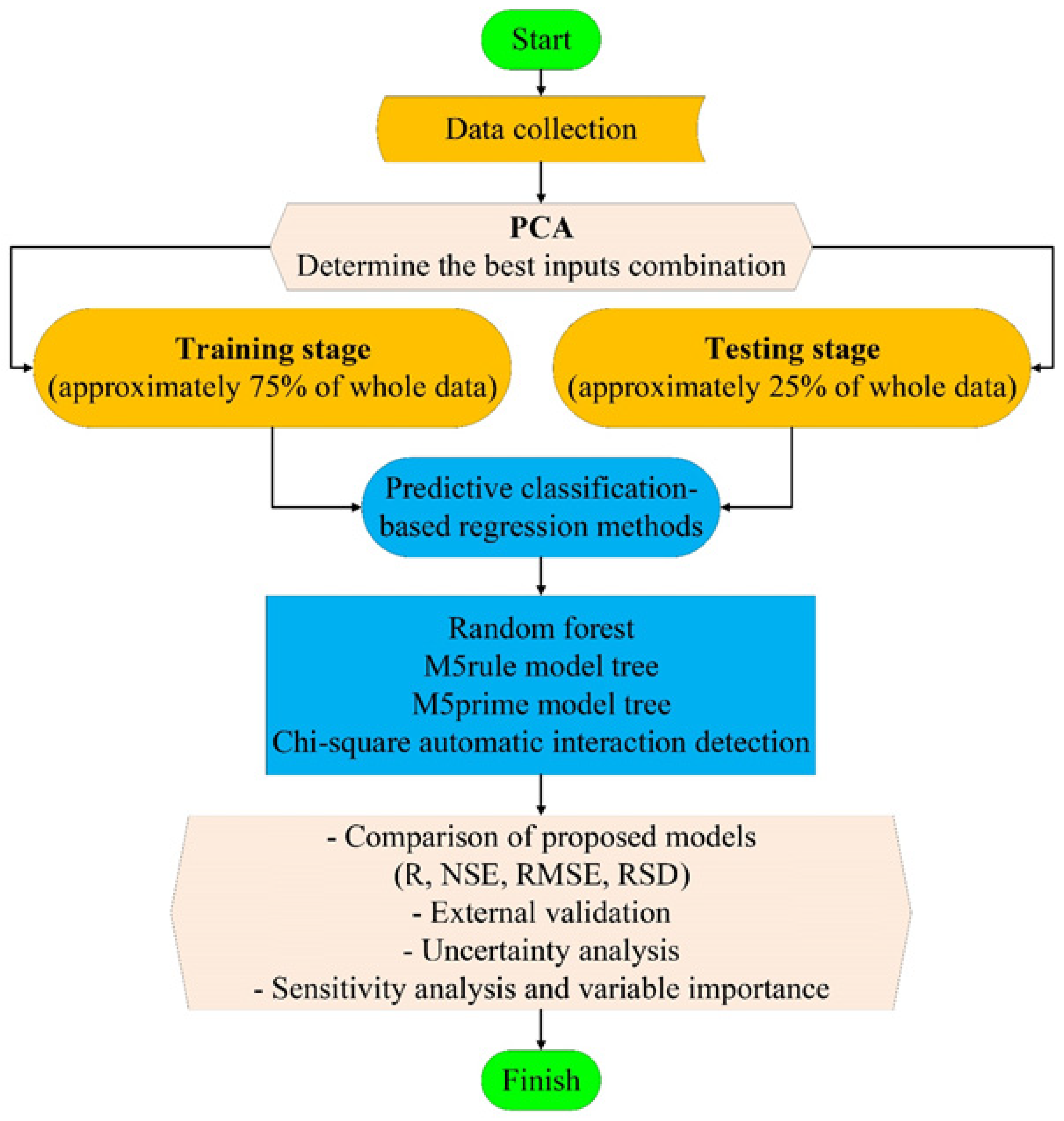
2. Materials and Methods

2.1. Theoretical Background and Data Description

Proper blend design is challenging in production of high-quality concrete [36]. Mechanical characteristics, economic benefit, and project constructability should be considered when designing RCCP blends [37]. Among the types of concrete, RCCP has become conventional due to the fact that it has a simple production process and it can be sourced quickly fast when producing a large structure. RCCP blends have lower cement weight (110–120 kg/m³), utilize natural aggregate, and are specified by the American Concrete Institute (ACI) standard 325-10R-95 as concrete incorporating less water, cement, and supplementary cementitious material [38].

A comprehensive and integrated dataset was utilized for building reliable simulation models based on ML techniques. A database was compiled from the open-source studies available in the literature [39,40,41,42,43,44,45,46,47,48,49,50,51,52,53,54,55,56,57,58,59,60]. From this database, models of the mechanical characteristics of RCCP were developed using 621, 326, and 290 data records for CS, TS, and FS of RCCP, respectively, at ages of 1, 3, 7, 28, 90, and 180 days. The gathered datasets contain information about the mixture components of RCCP in different combinations. For the ML techniques, the originally collected experimental data was randomized and categorized into two phases. The training (calibration) phase is implemented for learning and used to construct the models for CS, TS, and FS. The testing (validation) phase is performed to evaluate the capability of the developed models. For the development of the proposed methods, 75% of the data (466, 245, and 218 data records) for CS, TS, and FS, respectively, were used for the training phase, while the remainder (155, 81, and 72 data records) were used for testing phase of the classification-based regression methods. A schematic workflow of the simulation procedure of mechanical characteristics using ML-based models is presented in Figure 1.

2.2. Random Forest

Breiman [61] proposed RF, a nonparametric and classification-based regression method [62,63]. Instead of parametric models, many easy-to-interpret decision trees are incorporated in the RF model. By integration of the decision tree model results, a more comprehensive estimation technique can be attained. The objective of the current research is estimation of the mechanical properties of RCCP via the regression approach. The training steps of RF are as follows [61,62,63].

(a)

Based on the dataset, draw an instance that is chosen randomly with substitution.

(b)

Using the bootstrap instance, evolve a tree with these modifications: for each node, select the best randomized subset of m try descriptors (i.e., the number of predictors tried per each node). M try here has the role of a tuning a parameter in the RF algorithm. The tree is generated to its maximum size without pruning it.

(c)

Stage (b) is iterated until the user-manual numbers of trees (ntree) are grown on the basis of the bootstrap instance of observations. The final prediction values are determined by combining all individual tree outcomes [61]. After growing K trees {Tk(x)}, the regression explanatory variables in RF is stated by the following formula:

$$f\left(x\right)=\left[{\displaystyle \sum }_{K=1}^K{T}_k\left(x\right)\right]/K.$$

(1)

A new training set for each constructed RF regression tree is derived by replacing the original calibrating phase. Thus, after constructing a regression tree each time, through application of a randomized training sample, the out-of-bag instance is utilized for validating its precision [61].

$$GI(t_{X\left(xi\right)})=1-{\displaystyle \sum }_{j=1}^{m}f{\left(t_{X\left(xi\right),j}\right)}^2$$

(2)

The validation features improve the robustness of random forests due to the use of independent test data. The random forest algorithm is a feasible method for classification and regression purposes, and has many engineering applications, such as forecasting the properties of concrete [63].

2.3. M5 Rule Model Tree

The complex or hidden information in a dataset can be explored using the IF-THEN rules-based M5rule model tree, a commonly used model in machine learning for classification and regression tasks [64]. The M5rule model can create a single classification tree through repeated data splitting into groups while ensuring the uniformity in the output and applying some decision rules that are applicable to specific explanatory parameters [65]. The uniformity of the output can be estimated as the residual sum of the squares. The first stage involves the selection of the input variable for node splitting, which ensures the maximum uniformity of the resulting child nodes from the original parent nodes. The next step would be devoted to the selection of the other input variables which are the child nodes [66]. Having constructed the optimal regression tree, the next thing is to prune the tree to prevent overfitting, and for this purpose, a cross-validation process is applied for the selection of the model with the least prediction error.

2.4. M5 Prime Model Tree

The M5p model, which is based on linear regressions and decision trees, was first developed in 1992. A binary decision tree consists of the primary terminal node with extra leaf nodes, which provide a connection between input (independent) and output (dependent) parameters [67]. It is essential to bear in mind that decision trees are generally applied for categorical data, although it is also appropriate for quantitative type data [68]. The M5p model can be summarized in two main steps: (a) splitting input data to create a decision tree; it is reached when defining the standard deviation of each subset to find an appropriate primary node (parent node). Because of this step (splitting), the SD of the child node is smaller than the parent node; (b) testing each node in the decision tree to diminish the error. The standard deviation is calculated as:

$$SDR=sd\left(T\right)-{{\displaystyle \sum }}^{}\frac{\left|T_j\right|}{\left|T\right|}sd\left(T_j\right)$$

(3)

where sd represents the standard deviation, T is a set of examples that reach the primary node, and Tj represents the subset of patterns that possess the jth outcome of the potential set.

Thus, as stated above, based on different processes of splitting the input data, the most probable error-reducing node is chosen. For the overfitting problem in decision trees, pruning techniques were used for omitting subtrees. This pruning technique is based on methods of linear regression functions. One of the strengths of this model over the M5rule model is its efficiency in learning and treating problems with high complexity. One of the features of this model is that its regression functions do not have many variables. The M5p model has widespread applications in engineering, medical, and agricultural disciplines [69].

2.5. Chi-Square Automatic Interaction Detector

This CHAID model was first introduced by Kass for use in qualitative and classified quantitative variables [70]. As a modeling approach, this algorithm is suitable for establishing the relationship between a dependent parameter and several independent parameters. The CHAID model is mainly characterized by the following: (1) finding the influential parameters in the final result by applying a chi-square test of independence; (2) useful in the combination of effective variable groups [71]. This implies that CHAID employs the chi-squared independence test to examine the significance of independent parameters within a classification in comparison to the dependent parameters [72]. The chi-square statistic is expressed as follows:

$$X^2={{\displaystyle \sum }}^{}\frac{{\left(O_{ij}-E_{ij}\right)}^2}{E_{ij}}$$

(4)

where O_ij is the observed value, and E_ij is the predicted value. There are three stages in the CHAID model; merging, splitting, and stopping. The merging phase involves the application of the chi-square test to test the significance of each independent parameter. Each pair of dependent and independent parameters, as well as the probable tables, are subjected to this test. For the splitting stage, it initiates with the comparison of the calculated p-values of each independent parameter with the independent parameters that have the least p-value, followed by their selection as the node separator. In situations where no variable has a significant p-value, there will be no splitting stage and the final node will be determined as the node that precedes no branching [68]. The last stage (the stopping stage) begins with a repeat of the combination and analysis stages of all subsets. The process is terminated after all the subsets have been analyzed [71].

The formation of different parts in the CHAID model is represented by a classification tree diagram, where each dependent parameter is represented by a root, and the independent parameters are associated with significant p-values and are directly related with the root [72,73,74]. The weakness of this algorithm is that it cannot generate the best feasible divisions from the current parameters. More information on CHAID has been provided by [70,71,72,73].

2.6. Principal Component Analysis

Issues such as high dimensional input space, variables correlation, and insufficient training samples can create problems in the learning process, and the conditions might become worse when we want to spatially interpolate values for various locations within a city, but with few observation points [75]. It becomes inevitable to implement dimension reduction methods to reduce the number of correlated variables into the uncorrelated ones. Through application of PCA, while maintaining the highest variation and dispersion in the data, one can transform the input variables into a set of new uncorrelated variables called the principal components [76,77]. Equations (5) and (6) are used to provide linear transformation from the input space to the principal component space. Here, the orthogonal linear transformation matrix is defined by P, Z represents the original data matrix, according to which, each row denotes a variable, and Y represents the transformed matrix. In this matrix, each row denotes the uncorrelated principle components.

$$PZ=Y$$

(5)

$$\left[\begin{array}{c}{P}_{1.T_1}\dots P_{1.T_m}\\ .\\ .\\ .\\ P_{m.T_1}\dots P_{m.T_m}\end{array}\right]\left[\begin{array}{c}Z{T}_1\left(x_1\right)\dots Z{T}_1\left(x_n\right)\\ .\\ .\\ .\\ Z{T}_m\left(x_1\right)\dots Z{T}_m\left(x_n\right)\end{array}\right]=\left[\begin{array}{c}{y}_1\left(x_1\right)\dots y_1\left(x_n\right)\\ .\\ .\\ .\\ y_m\left(x_1\right)\dots y_m\left(x_n\right)\end{array}\right]$$

(6)

The transformation matrix (P) is obtained from the eigenvalues (λ1, λ2, …, λ1) of the covariance matrix of the original variables by applying PCA. The rows of this matrix represent the corresponding eigenvector. The eigenvectors specify the directions of the new space, and the eigenvalues specify their magnitude [77,78]. In order to find which eigenvector(s) could be removed without much affecting the information needed for building a subspace with lower dimensions, we should inspect their corresponding eigenvalues. Those eigenvectors which have smaller corresponding eigenvalues are those that have lower information on the data distribution and can be removed.

2.7. Statistical Criteria

In the present research, the following performance metrics (Equations (7)–(10)) were applied: correlation coefficient (R), Nash–Sutcliffe efficiency (NSE), root mean square error (RMSE), ratio of RMSE to standard deviation (RSD) [62,63,64]:

$$R=\frac{{{\displaystyle \sum }}_{i=1}^N\left(t_{exp}-\overline{t_{exp}}\right)·\left(t_{pre}-\overline{t_{pre}}\right)}{\sqrt{{{\displaystyle \sum }}_{i=1}^N{(t_{exp}-\overline{t_{exp}})}^2{{\displaystyle \sum }}_{i=1}^N{\left(t_{pre}-\overline{t_{pre}}\right)}^2}}$$

(7)

$$NSE=1-\frac{{{\displaystyle \sum }}_{i=1}^N{\left(t_{pre}-t_{exp}\right)}^2}{{{\displaystyle \sum }}_{i=1}^N{\left(t_{exp}-\overline{t_{exp}}\right)}^2}$$

(8)

$$RMSE=\sqrt{\frac{1}{N}{{\displaystyle \sum }}_{i=1}^N{\left(t_{pre}-t_{exp}\right)}^2}$$

(9)

$$RSD=\frac{RSME}{{{\displaystyle \sum }}_{i=1}^N\left(t_{exp}-\overline{t_{exp}}\right)}$$

(10)

where $t_{exp}$ and $t_{pre}$ denote the experimental and predicted target variable values, respectively. $\overline{t_{exp}}$ and $\overline{t_{pre}}$ are the mean of experimental and predicted target variable values, respectively. N denotes the total number of data. The R index, which is in the range of (0,1) (with R = 1 as the ideal value), shows the selected predictors suitability in predicting the target variable. NSE, with the range of (−∞, 1) and ideal value equal to unity, is used for assessing the capability of the proposed methods. Therefore, a value equal to unity shows perfect fitting between the actual and measured target values, and a negative value means bad performance of the model with respect to the arithmetic mean of the used models. RMSE and RSD with the range of (0, +∞) and ideal value of zero are used to assess the accuracy.

3. Application Results and Discussion

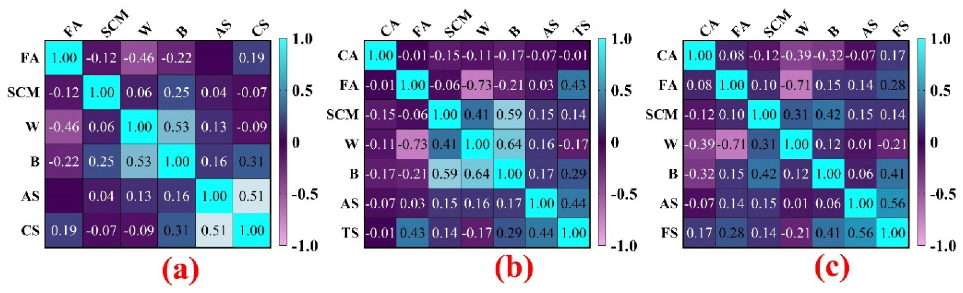
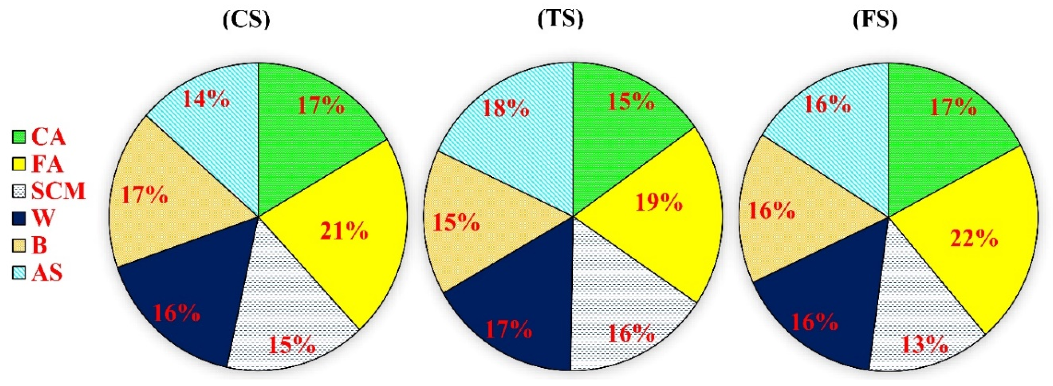
3.1. Selection of the Input Variables Using the PCA Technique

In this paper, to propagate the most effective combination of inputs for the simulation matrix of the mechanical characteristics, principal component analysis (PCA) based on dimensionality reduction was performed. The predictor variables affecting mechanical characteristics of RCCP of different ages are described as bellow:

$$f_c=f(CA,FA,C,SCM,B,W,\frac{W}{C},\frac{W}{B},\frac{SCM}{B},\frac{CA}{FA})$$

(11)

where CA (Kg/m³), FA (Kg/m³), C (Kg/m³), SCM (Kg/m³), B (Kg/m³), W (Kg/m³), W/C, W/B, SCM/B, and CA/FA are the coarse aggregate content, fine aggregate content, cement content, supplementary cementitious material content, binder content, water content, ratio of water to cement, ratio of water to binder, ratio of supplementary cementitious material to binder, and ratio of coarse to fine aggregate, respectively.

Table 1. Principal component analysis results to select optimal input combination.

Variable	PC1	PC2	PC3	PC4	PC5	PC6	PC8	PC9	PC10
CA	0.262	−0.942	0.187	0.086	−0.028	−0.001	0.000	0.000	0.000
FA	−0.959	−0.244	0.054	0.113	−0.065	−0.007	0.000	0.000	0.000
C	0.011	0.168	0.777	0.151	0.108	0.007	0.003	0.000	0.001
W/B	0.000	0.000	0.000	−0.001	0.000	0.007	−0.113	−0.993	0.019
SCM	0.046	−0.043	−0.546	0.600	0.069	0.004	−0.002	0.000	−0.002
W	0.072	0.082	0.081	0.187	−0.971	−0.056	−0.003	0.000	0.001
B	0.057	0.125	0.231	0.750	0.178	0.011	0.001	−0.001	−0.001
W/C	0.000	0.000	−0.003	0.001	−0.004	0.001	0.986	−0.115	−0.117
SCM/B	0.000	0.000	−0.002	0.001	0.000	0.000	0.118	0.006	0.993
CA/FA	−0.003	0.000	0.000	0.000	−0.058	0.998	0.000	0.007	0.000
EV	0.513	0.326	0.098	0.054	0.008	0.000	0.000	0.000	0.000
CS	0.513	0.839	0.937	0.991	1	1	1	1	1

reports the results of analysis consisting the contribution of 10 inputs to 10 PCs, the explained variance (EV) of each PC, and the cumulative sum (CS) of EV. PC1 represents 51.3% and the first four PCs represent 99.1% of total variance. The optimal input combinations are made bold in the table. The higher the EV, the better the combination of inputs.

The optimal combination of mixture proportions is calculated using Equation (11) using the PCA technique, as presented in Table 1. Five predictors provided the majority of the explained variance. Table 1 presents the values of the PCs and their variances. In Table 1, it can be seen that the volumetric and weighted forms of the experimental variables of CA, FA, SCM, W, and B, based on PC1, are the most effective independent predictor variables. Therefore, this combination of simulation variables along with age of specimens (AS) is used to construct the models to predict the mechanical characteristics of the concrete. The descriptive measures of the best combination of inputs for simulation of the mechanical characteristics of RCCP are presented in

Table 2. Statistical measures of independent and dependent variables for compressive strength (CS), tensile strength (TS), and flexural strength (FS).

Variables	Mean	Standard Deviation	Median	Kurtosis	Skewness	Minimum	Maximum
CA	1014.9	184.2	1095	−0.68	−0.62	585	1325
FA	855.87	225.7	807	−0.13	−0.22	272.5	1263
SCM	86.26	72.23	90	−0.7	0.44	0	272.5
W	129.29	39.57	117	7.5	2.26	78	336.25
B	311.6	66.44	295	8.34	2.12	200	672.5
AS	35.54	42.55	28	2.25	1.6	1	180
CS	33.276	16.553	31.4	−0.46	0.38	1.88	83
TS	3.1828	1.2761	3.2	−0.25	0.08	0.14	6.4
FS	4.498	1.864	4.55	−0.47	0.07	0.4	8.9

. The correlation coefficients of the selected independent variables for development of the proposed models are presented in Figure 2. According to the matrix, there are no significant relationships between the developed matrixes of CS, TS, and FS.

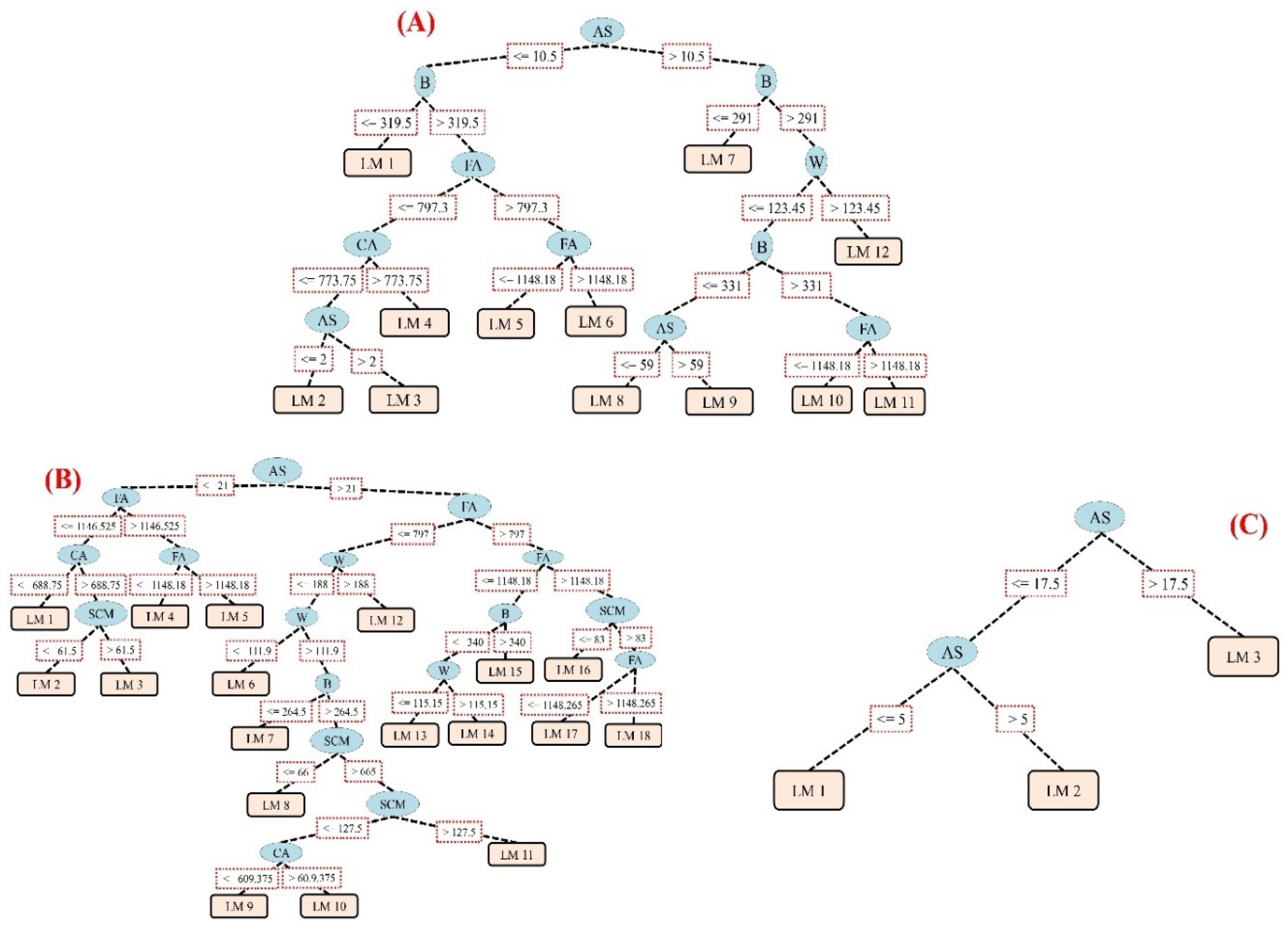
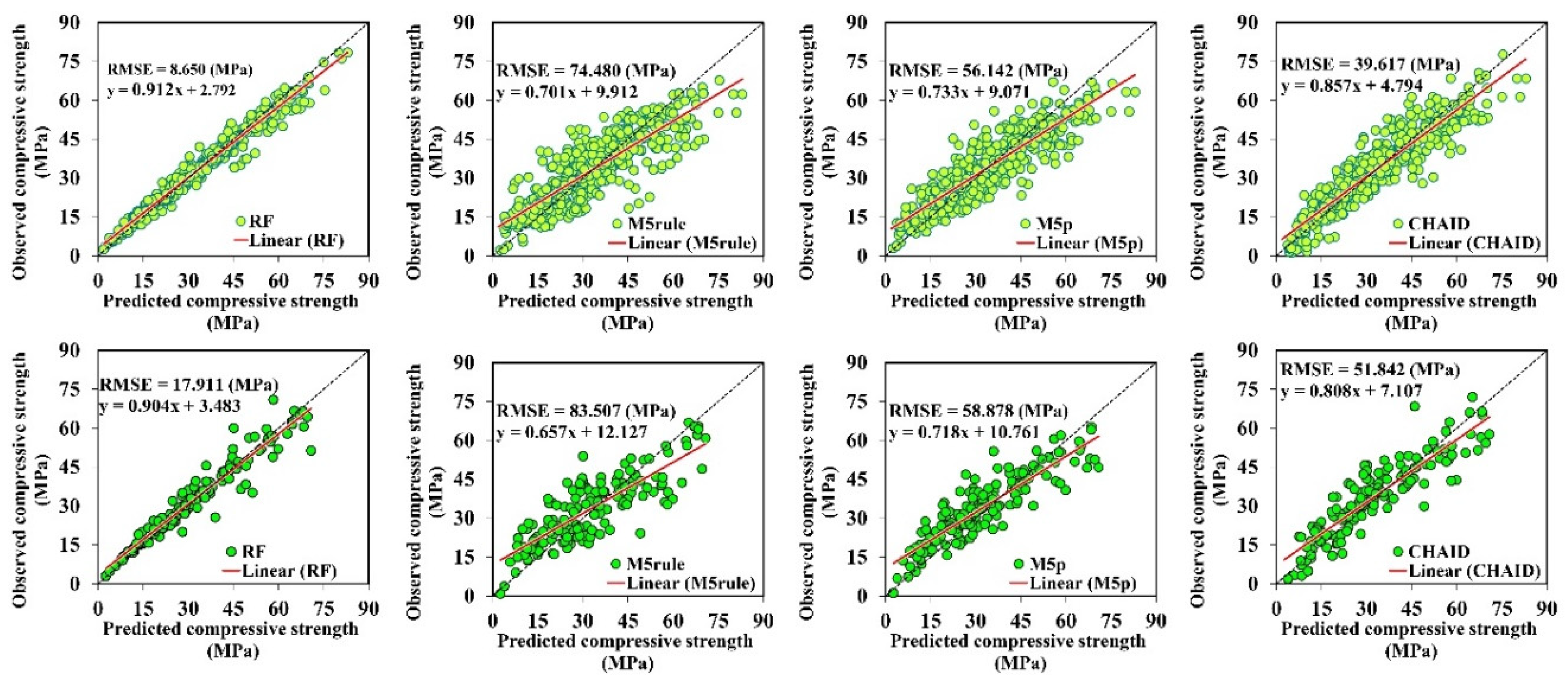
3.2. Estimation of RCCP Mechanical Characteristics Using Classification-Based Regression Methods

Application of the decision tree classification system, which is based on artificial intelligence, is a recent method proposed for solving engineering problems. The final properties of models are recaptured on the basis of network calibration. Then, the network can generalize those learned in a similar condition [67]. In the present study, the modelling methods included are four classification-based regression methods, namely RF, CHAID, M5rule, and M5prime, which were explored for the prediction of the characteristics of RCCP.

Definition of the matrix, consisting of CA, FA, SCM, W, B, and AS datasets, indicated the independent variables, and the dependent variables were CS, TS, and FS, which were used in each decision tree-based regression model. RF, M5rule, and M5p were performed using WEKA 3.9 and CHAID was implemented using STATISTICA software on an AMD A-12 9700, 10-core 2.5 GHz computer system.

To implement the RF model, the default Bagger algorithm was used with bag size percent set to 200, leaf number was set to eight, and delta criterion set to 0.1007. No mathematical formulation was utilized to fine the optimum number of trees. Commonly, a larger number of trees produces more precise results, but increases computational cost.

The M5tree procedure for simulation of RCCP properties was generated using a set of tuning parameters to initialize the proposed model. A pruning factor of 4.0 and smoothing option were selected to evaluate the performance of the M5 model towards proposing the mathematical linear formulations for RCCP. After classifying, the developed M5p model, consisting of six input variables and three output variables, was used for simulation of CS, TS, and FS of RCCP using 12, 18, and 3 rules, respectively. The proposed models have the optimum number of decision trees (linear models (LMs)) as this value achieves the lowest error in the training stage. These LMs (rules), on the basis of conditional sentences, are illustrated in Figure 3. Furthermore, the estimated CS, TS, and FS values are presented for AS smaller and greater than 10.5, 21, and 17.5 respectively, as in the M5p rule. Estimated coefficients for LMs based on proposed mathematical linear equation of RCCP properties (i.e., CS, TS, and FS) are presented in

Table A1. Input coefficients of M5p for CS estimation.

Linear Model	Coefficient
	CA	FA	SCM	W	B	AS	X
LM1	0.000	0.005	−0.043	−0.067	0.113	1.543	−11.878
LM2	0.010	0.002	−0.039	−0.078	0.082	1.681	−8.495
LM3	0.010	0.002	−0.042	−0.078	0.082	1.6815	−7.7941
LM4	0.010	−0.001	−0.024	−0.084	0.0819	0.7478	−2.6946
LM5	0.005	−0.013	−0.048	−0.220	0.265	1.068	−23.049
LM6	0.112	−0.023	−0.081	−0.149	0.148	1.317	−68.118
LM7	−0.016	0.001	−0.072	−0.100	0.251	0.104	−4.059
LM8	0.002	−0.004	−0.003	0.345	0.066	0.059	−15.986
LM9	0.002	−0.004	−0.003	0.293	0.066	0.058	−5.490
LM10	0.007	−0.006	−0.003	0.055	0.086	0.114	16.015
LM11	0.009	−31.824	−0.003	0.055	0.086	0.074	36.545
LM12	−0.012	−0.0003	0.049	−0.236	0.083	0.116	50.6158

X denoted the M5p intercept coefficient in LM.

,

Table A2. Input coefficients of M5p for TS estimation.

Linear Model	Coefficient
	CA	FA	SCM	W	B	AS	X
LM1	−0.004	0.0005	−0.002	−0.002	−0.029	0.213	7.607
LM2	0.001	0.0003	−0.006	−0.0008	0.002	0.015	0.004
LM3	0.0004	0.0003	0.003	0.0003	0.002	0.174	−0.0899
LM4	0.000	−0.006	−0.004	−0.003	0.003	0.125	9.550
LM5	0.000	−0.008	−0.007	−0.003	0.003	0.107	12.874
LM6	−0.0001	0.000	−0.003	−0.016	0.004	0.002	3.923
LM7	−0.0002	0.000	−0.004	−0.010	0.005	0.002	2.984
LM8	0.0001	−0.001	−0.003	−0.016	0.004	0.002	5.166
LM9	−0.0005	0.000	−0.004	−0.011	0.004	0.002	4.006
LM10	−0.0005	0.000	−0.004	−0.011	0.004	0.002	3.982
LM11	−0.0004	0.000	−0.004	−0.011	0.004	0.001	3.902
LM12	0.0004	−0.0003	−0.002	−0.002	0.003	0.004	2.258
LM13	0.001	0.001	0.0009	0.011	0.006	0.005	−1.933
LM14	0.001	0.001	0.0009	0.002	0.006	0.010	−1.058
LM15	0.003	0.001	0.001	0.002	0.007	0.003	−1.188
LM16	0.001	0.0004	0.001	0.0005	0.004	0.004	1.367
LM17	0.001	0.0006	−0.001	0.0005	0.004	0.003	1.295
LM18	0.001	0.0006	−0.001	0.0005	0.004	0.003	1.195

X denoted the M5p intercept coefficient in LM.

and

Table A3. Input coefficients of M5p for FS estimation.

Linear Model	Coefficient
	CA	FA	SCM	W	B	AS	X
LM1	0.001	0.0001	−0.009	−0.003	0.011	0.283	−1.899
LM2	0.002	0.0001	−0.001	−0.013	0.015	0.037	−1.207
LM3	0.003	0.0001	−0.0003	−0.0008	0.017	0.012	−3.863

X denoted the M5p intercept coefficient in LM.

in Appendix A. All inputs were included in the simulation of the mechanical characteristics of RCCP; they are significant in implementation of the developed LMs.

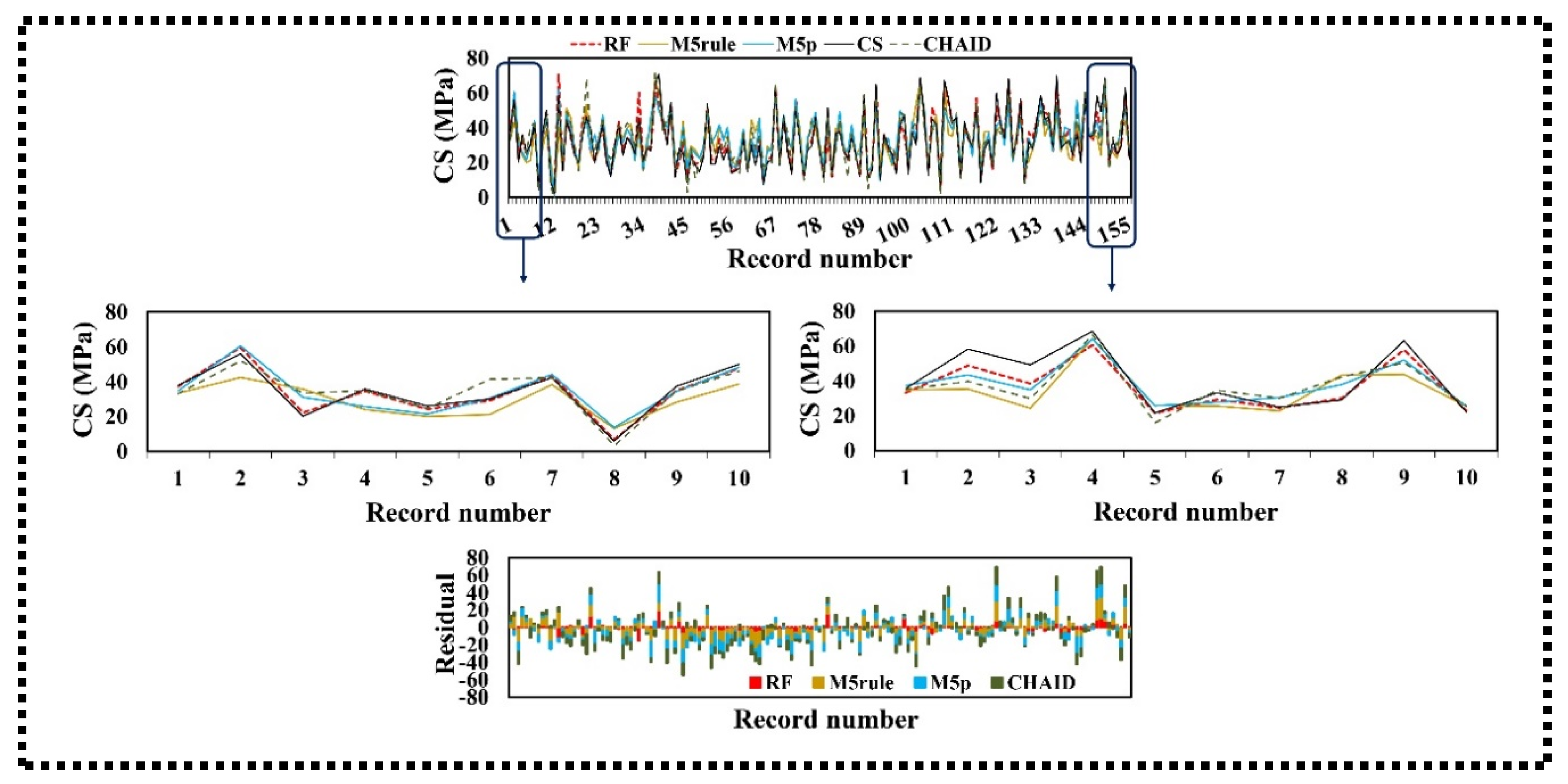
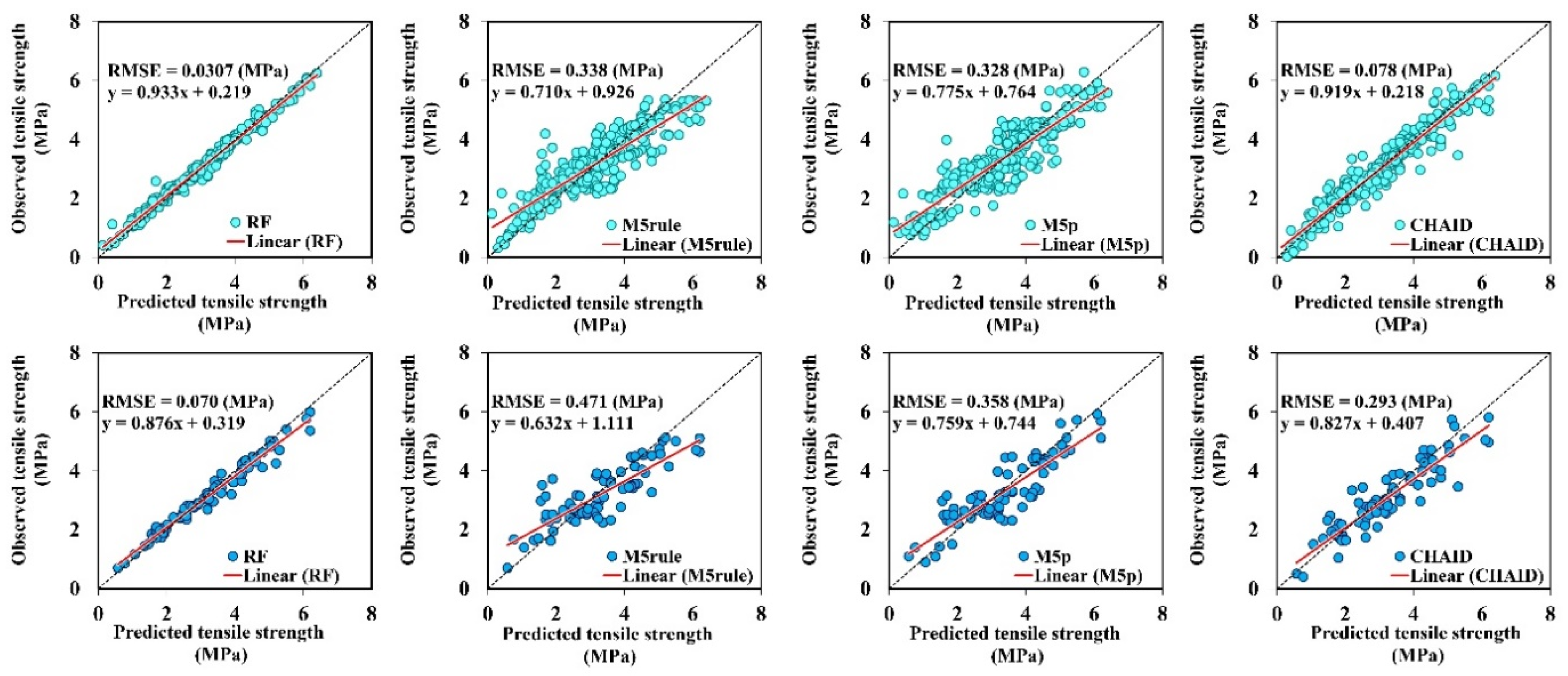
3.2.1. Compressive Strength

The observed and simulated compressive strength values estimated by the RF, M5rule, M5p, and CHAID models for RCCP are presented in Figure 4. As presented in Figure 4, the closer the ratio is to 1 (black and dotted line), the better the visual agreement between the observed CS and the simulated RF than other tree-based models. There were significant statistical correlations between the observed and simulated CS values for the four models under study. To compare the proposed tree-based models’ performances based on quantitative measures (i.e., NSE RSD, R, and RMSE),

Table 3. Predictive performance of the proposed models for CS prediction.

Phase	Proposed Models	Performance Metrics
		R	NSE	RMSE	RSD
Training	RF	0.986	0.968	8.650	0.561
	M5rule	0.855	0.731	74.480	5.460
	M5p	0.896	0.797	56.142	4.122
	CHAID	0.925	0.857	39.617	2.570
Testing	RF	0.965	0.931	17.911	1.181
	M5rule	0.828	0.680	83.507	6.499
	M5p	0.889	0.774	58.878	4.507
	CHAID	0.897	0.801	51.842	3.556

Bold text represents the best performance.

is presented. The evaluation metrics over the training phase reveal that RF simulated the CS with the highest precision (R = 0.986, NSE = 0.968 and minimum RSD = 0.561 MPa) in comparison with those estimated by the other ensemble tree-based techniques, such as CHAID (R = 0.925, NSE = 0.857 and RSD = 2.570 MPa). Moreover, the M5rule model attained lower performance in terms of R (0.855), NSE (0.731), RSME (74.480 MPa), and RSD (5.460 MPa) than M5p (R = 0.896, NSE = 0.797, RSME = 56.142 MPa, and RSD = 4.122 MPa).

In the testing phase, it is obvious that the CS values simulated by RF performed the best with the highest NSE (0.931) and lowest RSD (1.181 MPa) values in comparison with other ML methods. Figure 5 plots the observed and simulated CS of RCCP and their relative error using the tree-based techniques. The estimated CS of RF and CHAID models were in coherence with the observed data points. However, RF could only roughly simulate extreme CS values.

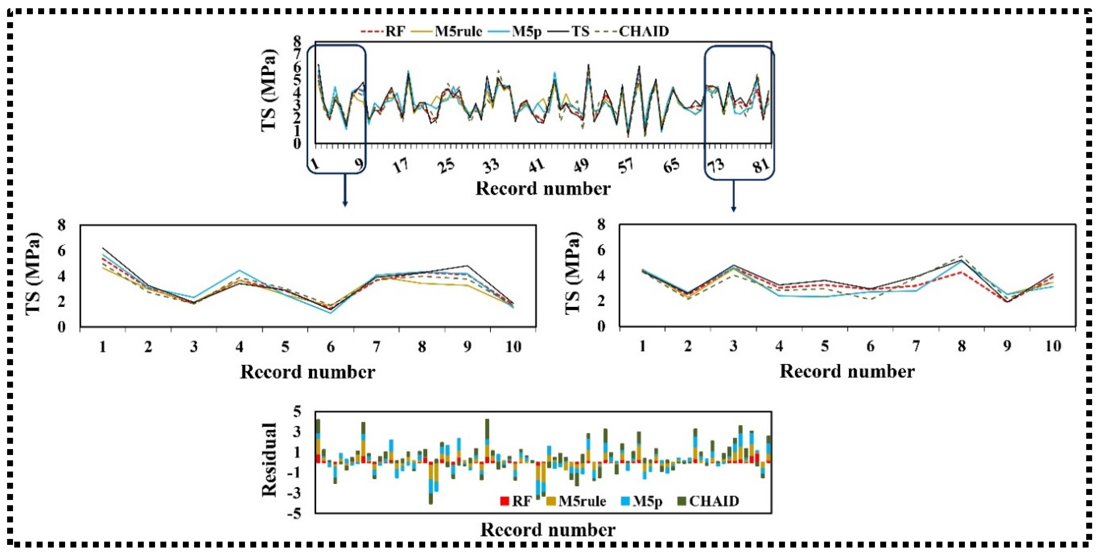
3.2.2. Tensile Strength

The performance indicators of the calibration and validation capability of estimating the tensile strength of RCCP using tree-based methods are reported in

Table 4. Predictive performance of the proposed models for TS prediction.

Phase	Proposed Models	Performance Metrics
		R	NSE	RMSE	RSD
Training	RF	0.991	0.981	0.030	0.025
	M5rule	0.892	0.791	0.338	0.320
	M5p	0.895	0.798	0.328	0.294
	CHAID	0.975	0.951	0.078	0.024
Testing	RF	0.984	0.955	0.070	0.062
	M5rule	0.850	0.706	0.471	0.500
	M5p	0.882	0.776	0.358	0.328
	CHAID	0.912	0.817	0.293	0.255

Bold text represents the best performance.

. According to Table 4, the RF model presented reliable performance in the training and testing phases. The statistical assessment for the validation subset of the proposed RF, M5rule, M5p, and CHAID techniques are (R = 0.984, NSE = 0.955 MPa, RMSE = 0.070 MPa and RSD = 0.062 MPa), (R = 0.850, NSE = 0.706 MPa, RMSE = 0.471 MPa and RSD = 0.500 MPa), (R = 0.882, NSE = 0.776 MPa, RMSE = 0.358 MPa and RSD = 0.328 MPa), and (R = 0.912, NSE = 0.817 MPa, RMSE = 0.293 MPa and RSD = 0.255 MPa), respectively. The graphical plots of subsets of the presented models are scattered in Figure 6. The presented tree-based models achieved acceptable simulation results for the TS of RCCP based on data correlated around the ideal line (1:1 line). Although a few data points developed by M5p and M5rule around the TS of 2–5 MPa indicated some small divergence from the 1:1 line, the results revealed that all of the tree-based methods provided high accuracy to simulate of tensile strength. The time series and residual plots for tree-based simulation and actual TS are presented in Figure 7. The RF model generated the minimum RMSE and outperforms the M5rule, M5p, and CHAID models for estimation of the TS of RCCP.

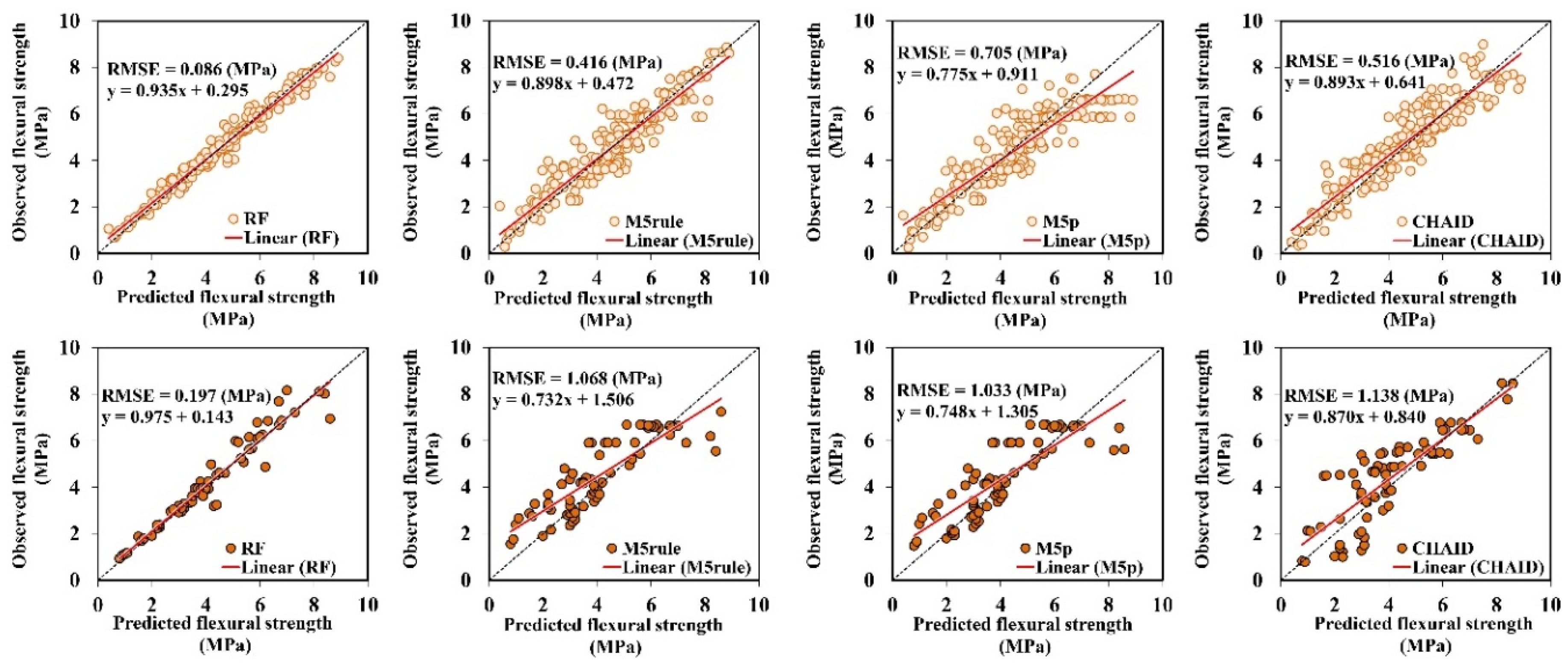
3.2.3. Flexural Strength

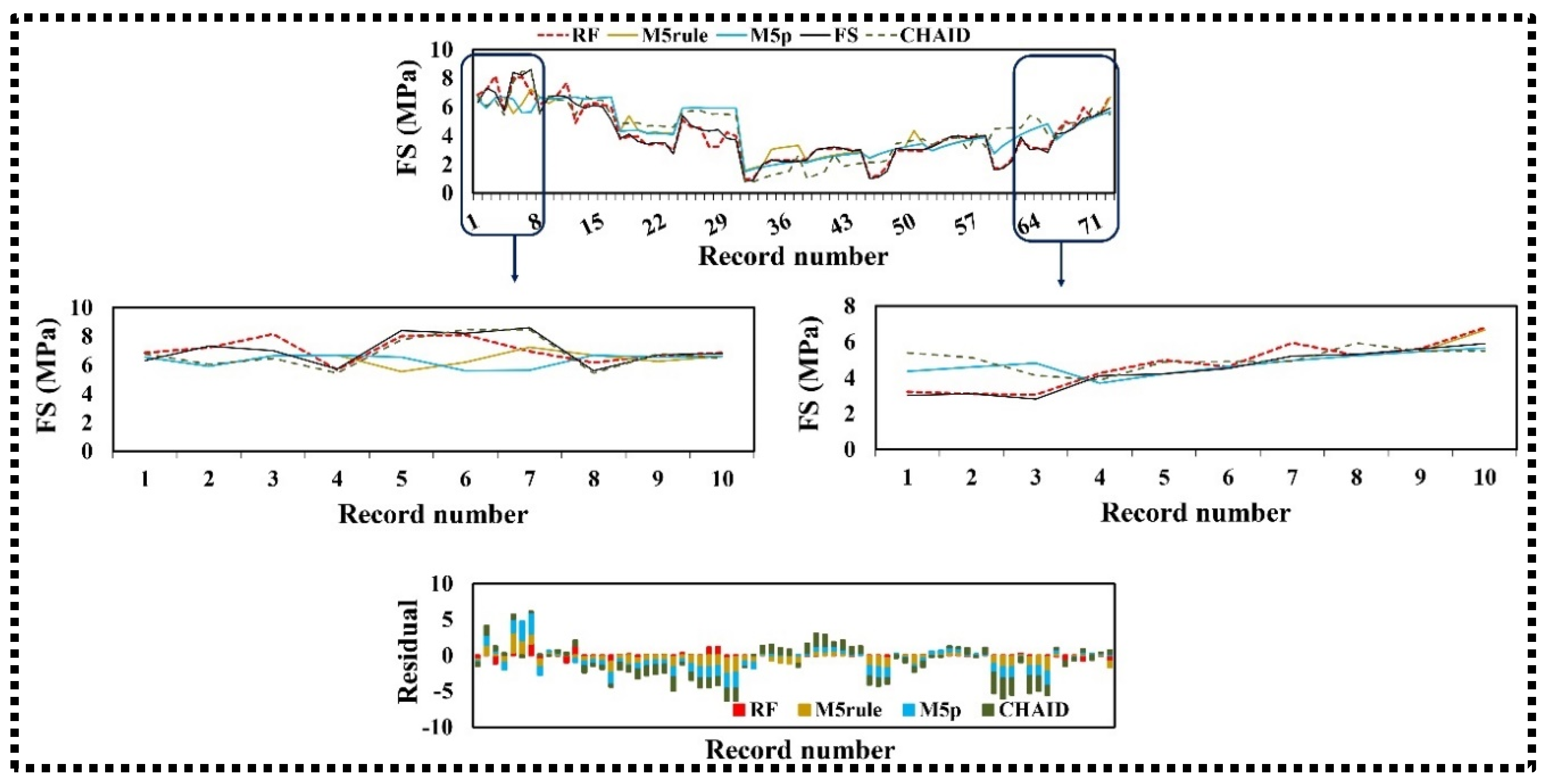
The applicability of tree-based models, namely RF, M5rule, M5p, and CHAID was investigated for estimation of the flexural strength of RCCP. The statistical evaluation of the developed models in the simulation of FS is presented considered in

Table 5. Predictive performance of the proposed models for FS prediction.

Phase	Proposed Models	Performance Metrics
		R	NSE	RMSE	RSD
Training	RF	0.988	0.974	0.086	0.049
	M5rule	0.937	0.878	0.416	0.234
	M5p	0.887	0.782	0.705	0.435
	CHAID	0.925	0.849	0.516	0.288
Testing	RF	0.970	0.939	0.197	0.108
	M5rule	0.853	0.673	1.068	0.689
	M5p	0.843	0.683	1.033	0.644
	CHAID	0.846	0.651	1.138	0.612

Bold text represents the best performance.

. In the 75%–25% data split of this study, the RF model outperformed the other ML methods in both training (R = 0.988 and RSD = 0.049 MPa) and testing stages (R = 0.970 and RSD = 0.108 MPa), respectively. RF has the lowest RMSE (0.197 MPa) and highest NSE (0.939); it enhanced the precision of testing phase in terms of NSE of the M5rule, M5p and CHAID by 28%, 27%, and 30%, respectively. Figure 8 and Figure 9 show the plots for comparison of the actual results with those of the four models inspired of tree-based regression methods. It can be shown in the aforementioned figures of the proposed models that the RF model has the highest accuracy in the simulation of FS during the training and testing steps. It is also evident from this plot that RF had a slightly higher precision in estimation of the local maximum and minimum FS values compared to the other ML methods.

3.3. Model Validity

External validation (EV) is used for comparison of the results of estimated and experimental data. Golbraikh and Tropsha [79] adopted new external validation criteria to assess the estimation precision of models according to the performance of validation data. EV means assessing the model performance with independent samples [80].

$${\displaystyle \sum }_{i=1}^n\frac{t_{obs}\times t_{pre}}{t_{pre}^2}$$

(12)

$$\frac{t_{obs}\times t_{pre}}{t_{obs}^2}$$

(13)

where $t_{obs}$ and $t_{pre}$ represent the experimental and estimated target values, respectively.

$$m=\left(R^2-R_0^2\right)/R^2<0.1$$

(14)

$$n=\left(R^2-R_0^{’2}\right)/R^2<0.1$$

(15)

Furthermore, Roy and Roy [81] used R_m (calculated by Equation (14)), a stabilization criterion, for external predictability of the models [81]. They found that an R_m value less than 0.5 shows an appropriate simulation.

$$R_m=R^2\times \left(1-\sqrt{\left|R^2-R_0^2\right|}\right)>0.5$$

(16)

The determination coefficients passing through the source between the estimated and experimental values ($R_0^2$), and conversely ($R_0^{’2}$), are derived using the following equations:

$$R_0^2=1-{\displaystyle \sum }_{i=1}^n{t}_{pre}^2{\left(1-k\right)}^2/{\displaystyle \sum }_{i=1}^n(t_{pre}-\overline{t_{pre}}{)}^2$$

(17)

$$R_0^{’2}=1-{\displaystyle \sum }_{i=1}^n{t}_{obs}^2{\left(1-k^{\prime }\right)}^2/{\displaystyle \sum }_{i=1}^n{(t_{obs}-{\overline{t}}_{obs})}^2$$

(18)

The validation indicator and the related performance of CS, TS, and FS prediction obtained by the various models are presented in

Table 6. Statistical measures of explained variance (EV) for all proposed models.

Model		K	K′	m	n	Rm
CS	RF	0.995	0.990	−0.071	−0.071	0.691
	M5rule	0.978	0.955	−0.452	−0.444	0.303
	M5p	0.971	0.984	−0.254	−0.261	0.436
	CHAID	0.986	0.983	−0.238	−0.240	0.552
TS	RF	1.035	0.961	−0.020	−0.019	0.834
	M5rule	1.038	0.927	−0.358	−0.328	0.354
	M5p	1.014	0.956	−0.282	−0.266	0.413
	CHAID	1.044	0.936	−0.181	−0.164	0.508
FS	RF	0.984	1.006	−0.060	−0.061	0.716
	M5rule	0.914	1.043	−0.278	−0.356	0.400
	M5p	0.934	1.018	−0.355	−0.402	0.353
	CHAID	0.910	1.043	−0.324	−0.380	0.370

. According to this table, the RF models for CS, TS, and FS, which yielded R_m = 0.691, R_m = 0.834, and R_m = 0716, respectively, satisfy the conditions and provide the best validation compared to the other models. In addition, the CART and M5tree values for CS (R_m = 0.187), TS (R_m = 0.195), and FS were less than the required value for R_m (R_m > 0.5). Thus, it is seen that RF shows highest validity for predicting the mechanical characteristics of RCCP.

Monte-Carlo simulation (MCS)-based uncertainty analysis is used for determining the randomness of model uncertainty. This method was first used by Ulam and Neman [82] in military projects for simulation of probabilistic events. It is well known that CS, TS, and FS contains various uncertainties, such as uncertainty of input variables and uncertainty of model parameters.

For this purpose, an investigation of quantitative uncertainty associated with output prediction rate (E) was performed using the RF, M5rule, M5p, and CHAID models. The MCS was performed for CS, TS, and FS values. The individual error of prediction was calculated for all the datasets (Equation (19)). Equations (20) and (21) are utilized for calculation of the mean $(\overline{e})$ and standard deviation $(S_e)$ of the estimation error, respectively [76]:

$$e_i={\log }_{10}\left(t^{pre}{}_i\right)-{\log }_{10}\left(t^{exp}{}_i\right)$$

(19)

$$\overline{e}={\displaystyle \sum }_{i=1}^n{e}_i$$

(20)

$$S_e=\sqrt{{\displaystyle \sum }_{i=1}^n\left(\frac{{\left(e_i-\overline{e}\right)}^2}{n-1}\right)}$$

(21)

In the above equations, n is the dataset length, and $t^{pre}$ and $t^{obs}$ denote the estimated and experimental target values, respectively. A positive mean prediction denotes an overestimated prediction of the target variable, and a negative one denotes an underestimated value of the target variable compared to the observed values. Thus, a confidence band could be drawn around the predicted error value through application of Wilson score approach [83,84]. Furthermore, $\pm 1.96S_e$ yields 95% confidence band around predicted P_i as follows:

$$\{P_i\times {10}^{-\overline{e}-1.96S_e},P_i\times {10}^{-\overline{e}+1.96S_e}\}$$

(22)

The outputs of this analysis, such as the uncertainty band width and mean absolute deviation (MAD), are given in

Table 7. Uncertainty quantification for all classification models.

Model		$\overline{\mathbf{e}}$	Se	Median	MAD	Uncertainty (%)
CS	RF	0.174	8.765	34.181	11.302	33.065
	M5rule	−0.017	3.313	32.539	12.530	38.509
	M5p	0.221	6.533	33.789	12.374	36.622
	CHAID	0.499	7.527	33.724	11.210	33.240
TS	RF	0.004	0.004	3.168	0.836	26.393
	M5rule	−0.038	0.361	3.091	0.973	31.507
	M5p	−0.012	0.201	3.108	0.943	30.346
	CHAID	0.048	0.578	3.116	0.883	28.348
FS	RF	−0.026	0.905	4.586	1.377	30.026
	M5rule	0.104	0.754	4.568	1.428	31.275
	M5p	0.008	0.338	4.563	1.455	31.896
	CHAID	0.188	0.798	4.806	1.447	30.119

. According to this table, the positive mean prediction error indicates that the predicted values calculated by all these methods are higher than the experimental values. It is seen that RF and CHAID methods for CS yielded the minimum (33.065% and 33.240) bandwidth uncertainties, respectively. Moreover, in other developed models, RF had the lowest uncertainty and satisfied the bandwidth criteria.

3.4. Sensitivity Analysis and Variable Importance

Sensitivity analysis (SA) of variables is a technique used to determine how different values of predictor variables will affect an output variable. For each independent variable, the SA% is calculated as follows [7]:

$$L_i=t_{max}\left(x_i\right)-t_{min}\left(x_i\right)$$

(23)

$$S{A}_i=\frac{L_i}{{{\displaystyle \sum }}_{j=1}^M{L}_i}\times 100$$

(24)

where $t_{max}$ and $t_{min}$ are the maximum and minimum of the estimated target over the i_th input domain, respectively, where other independent variable values are equal to their average values. The result of variable importance for the simulation of mechanical characteristics of RCCP is indicated in Figure 10 based on the RF model (best model). These figures show that the most effective variable in CS, TS, and FS estimation of RCCP is fine aggregate content.

4. Conclusions

In this research, classification-based regression methods based on the RF, M5rule, M5p, and CHAID techniques were applied as a ML tools to develop new predictive models of the mechanical characteristics of RCCP. The models were constructed using comprehensive datasets of RCCP design codes. Before development of the models, PCA was applied to determine the most important inputs predictors for data dimension reduction. RF and CHAID presented better performance for the training dataset compared to the other methods utilized in this research. The higher rank of RF and CHAID for the training data indicates that their flexibility, a result of combining multiple decision trees, is particularly useful for estimating the mechanical properties of RCCP. The performance of RF was significantly better than the other classification-based regression methods. This difference may be due to the larger diversity among the learned trees of RF, which is a consequence of RF’s implementation for randomized splitting at nodes. Typically, classification-based regression methods function better if there is notable diversity among the models [85,86]. However, the performance of the M5rule and M5p models was inferior to both RF and CHAID. This may be because the M5rule and M5p methods are more prone to overfitting, while RF and CHAID focus on variance reduction and consequently avoid overfitting. According to results of this research, the following conclusions can be drawn:

• Developing models based on RF, M5rule, M5p, and CHAID revealed that the CS, TS, and FS of RCCP are mainly related to the six inputs of CA, FA, SCM, W, B, and AS, as determined by PCA.
• The presented CS, TS, and FS-simulated values indicate that the RF method has greater precision compared with the other three tree-based techniques, with respect to R, NSE, RMSE, and RSD measures for the training and testing phases.
• The proposed RF and CHAID models met all of the required criteria of external validation.
• The Monte-Carlo uncertainty investigation of the implemented tree-based methods validated their robustness. Moreover, sensitivity analysis of variable importance revealed fine aggregate content to be the most important predictor influencing the mechanical characteristics of RCCP.

References

1. Hashemi, M.; Shafigh, P.; Bin Karim, M.R.; Atis, C.D. The effect of coarse to fine aggregate ratio on the fresh and hardened properties of roller-compacted concrete pavement. Constr. Build. Mater. 2018, 169, 553–566. [Google Scholar] [CrossRef]
2. Modarres, A.; Hesami, S.; Soltaninejad, M.; Madani, H. Application of coal waste in sustainable roller compacted concrete pavement-environmental and technical assessment. Int. J. Pavement Eng. 2016, 19, 748–761. [Google Scholar] [CrossRef]
3. Lam, M.N.-T.; Le, D.-H.; Jaritngam, S. Compressive strength and durability properties of roller-compacted concrete pavement containing electric arc furnace slag aggregate and fly ash. Constr. Build. Mater. 2018, 191, 912–922. [Google Scholar] [CrossRef]
4. Chhorn, C.; Kim, Y.K.; Hong, S.J.; Lee, S.W. Evaluation on compactibility and workability of roller-compacted concrete for pavement. Int. J. Pavement Eng. 2017, 20, 905–910. [Google Scholar] [CrossRef]
5. Adamu, M.; Mohammed, B.; Shafiq, N.; Liew, M.S. Durability performance of high volume fly ash roller compacted concrete pavement containing crumb rubber and nano silica. Int. J. Pavement Eng. 2018, 1–8. [Google Scholar] [CrossRef]
6. Adamu, M.; Mohammed, B.; Liew, M.S. Mechanical properties and performance of high volume fly ash roller compacted concrete containing crumb rubber and nano silica. Constr. Build. Mater. 2018, 171, 521–538. [Google Scholar] [CrossRef]
7. Ashrafian, A.; Gandomi, A.H.; Rezaie-Balf, M.; Emadi, M. An evolutionary approach to formulate the compressive strength of roller compacted concrete pavement. Measurement 2020, 152. [Google Scholar] [CrossRef]
8. Taheri Amiri, M.J.; Ashrafian, A.; Haghighi, F.R.; Javaheri Barforooshi, M. Prediction of the Compressive Strength of Self-compacting Concrete containing Rice Husk Ash using Data Driven Models. Modares Civ. Eng. J. 2019, 19, 196–206. [Google Scholar]
9. Rezaie-Balf, M.; Maleki, N.; Kim, S.; Ashrafian, A.; Babaie-Miri, F.; Kim, N.W.; Chung, I.-M.; Alaghmand, S. Forecasting Daily Solar Radiation Using CEEMDAN Decomposition-Based MARS Model Trained by Crow Search Algorithm. Energies 2019, 12, 1416. [Google Scholar] [CrossRef] [Green Version]
10. Ashrafian, A.; Taheri, A.M.J.; Haghighi, F. Modeling the Slump Flow of Self-Compacting Concrete Incorporating Metakaolin Using Soft Computing Techniques. J. Syst. Control Eng. 2019, 5–20. [Google Scholar] [CrossRef]
11. Amlashi, A.T.; Abdollahi, S.M.; Goodarzi, S.; Ghanizadeh, A.R. Soft computing based formulations for slump, compressive strength, and elastic modulus of bentonite plastic concrete. J. Clean. Prod. 2019, 230, 1197–1216. [Google Scholar] [CrossRef]
12. Gholampour, A.; Gandomi, A.H.; Ozbakkaloglu, T. New formulations for mechanical properties of recycled aggregate concrete using gene expression programming. Constr. Build. Mater. 2017, 130, 122–145. [Google Scholar] [CrossRef]
13. Asteris, P.G.; Armaghani, D.J.; Hatzigeorgiou, G.D.; Karayannis, C.G.; Pilakoutas, K. Predicting the shear strength of reinforced concrete beams using Artificial Neural Networks. Eng. Struct. 2019, 24, 469–488. [Google Scholar]
14. Ly, H.B.; Pham, B.T.; Dao, D.V.; Le, V.M.; Le, L.M.; Le, T.T. Improvement of ANFIS Model for Prediction of Compressive Strength of Manufactured Sand Concrete. Appl. Sci. 2019, 9, 3841. [Google Scholar] [CrossRef] [Green Version]
15. Sun, J.; Zhang, J.; Gu, Y.; Huang, Y.; Sun, Y.; Ma, G. Prediction of permeability and unconfined compressive strength of pervious concrete using evolved support vector regression. Constr. Build. Mater. 2019, 207, 440–449. [Google Scholar] [CrossRef]
16. Ashrafian, A.; Shokri, F.; Amiri, M.J.T.; Yaseen, Z.M.; Rezaie-Balf, M. Compressive strength of Foamed Cellular Lightweight Concrete simulation: New development of hybrid artificial intelligence model. Constr. Build. Mater. 2020, 230, 117048. [Google Scholar] [CrossRef]
17. Deng, F.; He, Y.; Zhou, S.; Yu, Y.; Cheng, H.; Wu, X. Compressive strength prediction of recycled concrete based on deep learning. Constr. Build. Mater. 2018, 175, 562–569. [Google Scholar] [CrossRef]
18. Karballaeezadeh, N.; Zaremotekhases, F.; Shamshirband, S.; Mosavi, A.; Nabipour, N.; Csiba, P.; Várkonyi-Kóczy, A.R. Intelligent Road Inspection with Advanced Machine Learning; Hybrid Prediction Models for Smart Mobility and Transportation Maintenance Systems. Energies 2020, 13, 1718. [Google Scholar] [CrossRef] [Green Version]
19. Shahmansouri, A.A.; Bengar, H.A.; Jahani, E. Predicting compressive strength and electrical resistivity of eco-friendly concrete containing natural zeolite via GEP algorithm. Constr. Build. Mater. 2019, 229, 116883. [Google Scholar] [CrossRef]
20. Feng, D.-C.; Liu, Z.-T.; Wang, X.-D.; Chen, Y.; Chang, J.-Q.; Wei, D.-F.; Jiang, Z. Machine learning-based compressive strength prediction for concrete: An adaptive boosting approach. Constr. Build. Mater. 2020, 230, 117000. [Google Scholar] [CrossRef]
21. Iqbal, M.F.; Liu, Q.-F.; Azim, I.; Zhu, X.; Yang, J.; Javed, M.F.; Rauf, M. Prediction of mechanical properties of green concrete incorporating waste foundry sand based on gene expression programming. J. Hazard. Mater. 2020, 384, 121322. [Google Scholar] [CrossRef]
22. Asteris, P.G.; Ashrafian, A.; Rezaie-Balf, M. Prediction of the compressive strength of self-compacting concrete using surrogate models. Comput. Concr. 2019, 24, 137–150. [Google Scholar]
23. Golafshani, E.M.; Behnood, A.; Arashpour, M. Predicting the compressive strength of normal and High-Performance Concretes using ANN and ANFIS hybridized with Grey Wolf Optimizer. Constr. Build. Mater. 2020, 232, 117266. [Google Scholar] [CrossRef]
24. Yoon, J.Y.; Kim, H.; Lee, Y.-J.; Sim, S.-H. Prediction Model for Mechanical Properties of Lightweight Aggregate Concrete Using Artificial Neural Network. Materials 2019, 12, 2678. [Google Scholar] [CrossRef] [PubMed] [Green Version]
25. Van Dao, D.; Ly, H.-B.; Trinh, S.H.; Le, T.-T.; Pham, B.T. Artificial Intelligence Approaches for Prediction of Compressive Strength of Geopolymer Concrete. Materials 2019, 12, 983. [Google Scholar] [CrossRef] [Green Version]
26. Sun, L.; Koopialipoor, M.; Armaghani, D.J.; Tarinejad, R.; Tahir, M.M. Applying a meta-heuristic algorithm to predict and optimize compressive strength of concrete samples. Eng. Comput. 2019, 1–13. [Google Scholar] [CrossRef]
27. Moayedi, H.; Kalantar, B.; Foong, L.K.; Bui, T.; Motevalli, A.; Bui, D.T. Application of Three Metaheuristic Techniques in Simulation of Concrete Slump. Appl. Sci. 2019, 9, 4340. [Google Scholar] [CrossRef] [Green Version]
28. Hassan, M.; Khalil, A.; Kaseb, S.; Kassem, M. Exploring the potential of tree-based ensemble methods in solar radiation modeling. Appl. Energy 2017, 203, 897–916. [Google Scholar] [CrossRef]
29. Fan, J.; Yue, W.; Wu, L.; Zhang, F.; Cai, H.; Wang, X.; Lu, X.; Xiang, Y. Evaluation of SVM, ELM and four tree-based ensemble models for predicting daily reference evapotranspiration using limited meteorological data in different climates of China. Agric. For. Meteorol. 2018, 263, 225–241. [Google Scholar] [CrossRef]
30. Behnood, A.; Olek, J.; Glinicki, M.A. Predicting modulus elasticity of recycled aggregate concrete using M5′ model tree algorithm. Constr. Build. Mater. 2015, 94, 137–147. [Google Scholar] [CrossRef]
31. Behnood, A.; Behnood, V.; Gharehveran, M.M.; Alyamaç, K.E. Prediction of the compressive strength of normal and high-performance concretes using M5P model tree algorithm. Constr. Build. Mater. 2017, 142, 199–207. [Google Scholar] [CrossRef]
32. Han, Q.; Gui, C.; Xu, J.; Lacidogna, G. A generalized method to predict the compressive strength of high-performance concrete by improved random forest algorithm. Constr. Build. Mater. 2019, 226, 734–742. [Google Scholar] [CrossRef]
33. Mohamed, O.A.; Ati, M.; Najm, O.F. Predicting Compressive Strength of Sustainable Self-Consolidating Concrete Using Random Forest. In Key Engineering Materials; Trans Tech Publications: New York, NY, USA, 2017; Volume 744, pp. 141–145. [Google Scholar] [CrossRef]
34. Ashrafian, A.; Amiri, M.J.T.; Rezaie-Balf, M.; Ozbakkaloglu, T.; Lotfi-Omran, O. Prediction of compressive strength and ultrasonic pulse velocity of fiber reinforced concrete incorporating nano silica using heuristic regression methods. Constr. Build. Mater. 2018, 190, 479–494. [Google Scholar] [CrossRef]
35. Gholampour, A.; Mansouri, I.; Kisi, O.; Ozbakkaloglu, T. Evaluation of mechanical properties of concretes containing coarse recycled concrete aggregates using multivariate adaptive regression splines (MARS), M5 model tree (M5Tree), and least squares support vector regression (LSSVR) models. Neural Comput. Appl. 2018, 32, 295–308. [Google Scholar] [CrossRef]
36. AzariJafari, H.; Amiri, M.J.T.; Ashrafian, A.; Rasekh, H.; Barforooshi, M.J.; Berenjian, J. Ternary blended cement: An eco-friendly alternative to improve resistivity of high-performance self-consolidating concrete against elevated temperature. J. Clean. Prod. 2019, 223, 575–586. [Google Scholar] [CrossRef]
37. Ramezanianpour, A.A.; Mohammadi, A.; Dehkordi, E.R.; Chenar, Q.B. Mechanical properties and durability of roller compacted concrete pavements in cold regions. Constr. Build. Mater. 2017, 146, 260–266. [Google Scholar] [CrossRef]
38. Kokubu, K.; Anzaki, Y. State of the Art Report on Roller Compacted Concrete Pavements. Concr. J. 1989, 27, 22–30. [Google Scholar] [CrossRef] [Green Version]
39. Rao, S.K.; Sravana, P.; Rao, T.C. Strength and Compaction Characteristics of Fly Ash Roller Compacted Concrete. Int. J. Sci. Res. Knowl. 2015, 3, 260–269. [Google Scholar] [CrossRef]
40. Mardani-Aghabaglou, A.; Ramyar, K. Mechanical properties of high-volume fly ash roller compacted concrete designed by maximum density method. Constr. Build. Mater. 2013, 38, 356–364. [Google Scholar] [CrossRef]
41. Pavan, S.; Rao, S.K. Effect of Fly ash on Strength Characteristics of Roller Compacted Concrete Pavement. IOSR J. Mech. Civ. Eng. 2014, 11, 4–8. [Google Scholar] [CrossRef]
42. Atiş, C.D.; Sevim, U.; Özcan, F.; Bilim, C.; Karahan, O.; Tanrikulu, A.; Eksi, A. Strength properties of roller compacted concrete containing a non-standard high calcium fly ash. Mater. Lett. 2004, 58, 1446–1450. [Google Scholar] [CrossRef]
43. Tangtermsirikul, S.; Kaewkhluab, T.; Jitvutikrai, P. A compressive strength model for roller-compacted concrete with fly ash. Mag. Concr. Res. 2004, 56, 35–44. [Google Scholar] [CrossRef]
44. Rao, S.K.; Sravana, P.; Rao, T.C. Experimental studies in Ultrasonic Pulse Velocity of roller compacted concrete pavement containing fly ash and M-sand. Int. J. Pavement Res. Technol. 2016, 9, 289–301. [Google Scholar] [CrossRef] [Green Version]
45. Cao, C.; Sun, W.; Qin, H. The analysis on strength and fly ash effect of roller-compacted concrete with high volume fly ash. Cem. Concr. Res. 2000, 30, 71–75. [Google Scholar] [CrossRef]
46. Rao, S.K.; Sravana, P.; Rao, T.C. Investigation on pozzolanic effect of Fly ash in Roller Compacted Concrete pavement. IRACST-Eng. Sci. Technol. Int. J. 2015, 5, 202–206. [Google Scholar]
47. Ghahari, S.; Mohammadi, A.; Ramezanianpour, A. Performance assessment of natural pozzolan roller compacted concrete pavements. Case Stud. Constr. Mater. 2017, 7, 82–90. [Google Scholar] [CrossRef]
48. Mohammed, B.S.; Adamu, M. Mechanical performance of roller compacted concrete pavement containing crumb rubber and nano silica. Constr. Build. Mater. 2018, 159, 234–251. [Google Scholar] [CrossRef]
49. Debbarma, S.; Ransinchung, G.D.; Singh, S. Feasibility of roller compacted concrete pavement containing different fractions of reclaimed asphalt pavement. Constr. Build. Mater. 2019, 199, 508–525. [Google Scholar] [CrossRef]
50. Fardin, H.E.; Santos, A.G. Roller Compacted Concrete with Recycled Concrete Aggregate for Paving Bases. Sustainability 2020, 12, 3154. [Google Scholar] [CrossRef] [Green Version]
51. Lam, M.N.-T.; Jaritngam, S.; Le, D.-H. EAF Slag Aggregate in Roller-Compacted Concrete Pavement: Effects of Delay in Compaction. Sustainability 2018, 10, 1122. [Google Scholar] [CrossRef] [Green Version]
52. Mohammadzadeh S., D.; Kazemi, S.-F.; Nasseralshariati, E.; Tah, J.H.M. Prediction of Compression Index of Fine-Grained Soils Using a Gene Expression Programming Model. Infrastructures 2019, 4, 26. [Google Scholar] [CrossRef] [Green Version]
53. Shamsaei, M.; Aghayan, I.; Kazemi, K.A. Experimental investigation of using cross-linked polyethylene waste as aggregate in roller compacted concrete pavement. J. Clean. Prod. 2017, 165, 290–297. [Google Scholar] [CrossRef]
54. Hesami, S.; Modarres, A.; Soltaninejad, M.; Madani, H. Mechanical properties of roller compacted concrete pavement containing coal waste and limestone powder as partial replacements of cement. Constr. Build. Mater. 2016, 111, 625–636. [Google Scholar] [CrossRef]
55. Nabipour, N.; Karballaeezadeh, N.; Dineva, A.; Mosavi, A.; Mohammadzadeh S., D.; Shamshirband, S. Comparative Analysis of Machine Learning Models for Prediction of Remaining Service Life of Flexible Pavement. Mathematics 2019, 7, 1198. [Google Scholar] [CrossRef] [Green Version]
56. Rao, S.K.; Sravana, P.; Rao, T.C. Abrasion resistance and mechanical properties of Roller Compacted Concrete with GGBS. Constr. Build. Mater. 2016, 114, 925–933. [Google Scholar] [CrossRef]
57. Karballaeezadeh, N.; Mohammadzadeh S., D.; Moazami, D.; Nabipour, N.; Mosavi, A.; Reuter, U. Smart Structural Health Monitoring of Flexible Pavements Using Machine Learning Methods. Preprints 2020, 2020040029. [Google Scholar] [CrossRef]
58. Karballaeezadeh, N.; Mohammadzadeh S., D.; Shamshirband, S.; Hajikhodaverdikhan, P.; Mosavi, A.; Chau, K.W. Prediction of remaining service life of pavement using an optimized support vector machine (case study of Semnan–Firuzkuh road). Eng. Appl. Comput. Fluid Mech. 2019, 13, 188–198. [Google Scholar]
59. Sheikh Khozani, Z.; Sheikhi, S.; Mohtar, W.H.M.W.; Mosavi, A. Forecasting shear stress parameters in rectangular channels using new soft computing methods. PLoS ONE 2020, 15, e0229731. [Google Scholar] [CrossRef] [Green Version]
60. Rashad, A.M. A preliminary study on the effect of fine aggregate replacement with metakaolin on strength and abrasion resistance of concrete. Constr. Build. Mater. 2013, 44, 487–495. [Google Scholar] [CrossRef]
61. Breiman, L. Random forests. Mach. Learn. 2001, 45, 5–32. [Google Scholar] [CrossRef] [Green Version]
62. Adusumilli, S.; Bhatt, D.; Wang, H.; Bhattacharya, P.; Devabhaktuni, V. A low-cost INS/GPS integration methodology based on random forest regression. Expert Syst. Appl. 2013, 40, 4653–4659. [Google Scholar] [CrossRef]
63. Zhou, J.; Shi, X.; Du, K.; Qiu, X.; Li, X.; Mitri, H. Feasibility of Random-Forest Approach for Prediction of Ground Settlements Induced by the Construction of a Shield-Driven Tunnel. Int. J. Géoméch. 2017, 17, 04016129. [Google Scholar] [CrossRef]
64. Zhou, J.; Li, X.; Mitri, H. Comparative performance of six supervised learning methods for the development of models of hard rock pillar stability prediction. Nat. Hazards 2015, 79, 291–316. [Google Scholar] [CrossRef]
65. Troncoso, A.; Salcedo-Sanz, S.; Casanova-Mateo, C.; Riquelme, J.C.; Prieto, L. Local models-based regression trees for very short-term wind speed prediction. Renew. Energy 2015, 81, 589–598. [Google Scholar] [CrossRef]
66. Arnett, F.C.; Edworthy, S.M.; Bloch, D.A.; McShane, D.J.; Fries, J.F.; Cooper, N.S.; Healey, L.A.; Kaplan, S.R.; Liang, M.H.; Luthra, H.S.; et al. The american rheumatism association 1987 revised criteria for the classification of rheumatoid arthritis. Arthritis Rheum. 1988, 31, 315–324. [Google Scholar] [CrossRef]
67. Quinlan, J.R. Learning with Continuous Classes. In Proceedings of the 5th Australian Joint Conference on Artificial Intelligence, Hobart, Tasmania, Australia, 16–18 November 1992. [Google Scholar]
68. Mitchell, T.M. Machine learning and data mining. Commun. ACM 1999, 42, 30–36. [Google Scholar] [CrossRef]
69. Abdelkader, S.S.; Grolinger, K.; Capretz, M.A. Predicting Energy Demand Peak Using M5 Model Trees. In Proceedings of the 2015 IEEE 14th International Conference on Machine Learning and Applications (ICMLA), Miami, FL, USA, 9–11 December 2015; pp. 509–514. [Google Scholar]
70. Attar, N.F.; Pham, Q.B.; Nowbandegani, S.; Rezaie-Balf, M.; Fai, C.M.; Ahmed, A.N.; Pipelzadeh, S.; Tran, D.D.; Nhi, P.T.T.; Dao, N.-K.; et al. Enhancing the Prediction Accuracy of Data-Driven Models for Monthly Streamflow in Urmia Lake Basin Based upon the Autoregressive Conditionally Heteroskedastic Time-Series Model. Appl. Sci. 2020, 10, 571. [Google Scholar] [CrossRef] [Green Version]
71. Kass, G.V. An Exploratory Technique for Investigating Large Quantities of Categorical Data. J. R. Stat. Soc. Ser. C Appl. Stat. 1980, 29, 119. [Google Scholar] [CrossRef]
72. Kamber, M.; Pei, J. Data Mining; Morgan Kaufmann: New York, NY, USA, 2006. [Google Scholar]
73. Sharp, A. The Performance of Segmentation Variables: A Comparative Study. Ph.D. Thesis, University of Otago, Otago, New Zealand, 1998. [Google Scholar]
74. Gallagher, C.A.; Monroe, H.M.; Fish, J.L. An Iterative Approach to Classification Analysis. J. Appl. Stat. 2000, 29, 256–266. [Google Scholar]
75. Lungu, C.; Ersali, S.; Szefler, B.; Pîrvan-Moldovan, A.; Basak, S.; Diudea, M. Dimensionality of big data sets explored by Cluj descriptors. Studia Univ. Babeș-Bolyai Chem. 2017, 62, 197–204. [Google Scholar] [CrossRef]
76. Jolliffe, I.T. Principal Component Analysis, 2nd ed.; Springer: New York, NY, USA, 2002; ISBN 978-0-387-95442-4. [Google Scholar]
77. Gosav, S.; Praisler, M.; Birsa, L.M. Principal Component Analysis Coupled with Artificial Neural Networks—A Combined Technique Classifying Small Molecular Structures Using a Concatenated Spectral Database. Int. J. Mol. Sci. 2011, 12, 6668–6684. [Google Scholar] [CrossRef] [PubMed] [Green Version]
78. Defernez, M.; Kemsley, E.K. Avoiding overfitting in the analysis of high-dimensional data with artificial neural networks (ANNs). Analyst 1999, 124, 1675–1681. [Google Scholar] [CrossRef]
79. Golbraikh, A.; Tropsha, A. Beware of q2! J. Mol. Graph. Model. 2002, 20, 269–276. [Google Scholar] [CrossRef]
80. Sattar, A.M.A. Gene Expression Models for the Prediction of Longitudinal Dispersion Coefficients in Transitional and Turbulent Pipe Flow. J. Pipeline Syst. Eng. Pr. 2014, 5, 04013011. [Google Scholar] [CrossRef]
81. Roy, P.P.; Roy, K. On Some Aspects of Variable Selection for Partial Least Squares Regression Models. QSAR Comb. Sci. 2008, 27, 302–313. [Google Scholar] [CrossRef]
82. Landau, D.P. An Introduction To Monte Carlo Methods in Statistical Physics; World Scientific Pub Co Pte Ltd.: Singapore, 2005; pp. 53–91. [Google Scholar]
83. Newcombe, R.G. Two-sided confidence intervals for the single proportion: Comparison of seven methods. Stat. Med. 1998, 17, 857–872. [Google Scholar] [CrossRef]
84. Abessi, O.; Eshtehardian, E.; Haghighi, F.; Taheri, M.J. Optimization of Time, Cost, and Quality in Critical Chain Method Using Simulated Annealing (RESEARCH NOTE). Int. J. Eng. 2017, 30, 627–635. [Google Scholar]
85. Kuncheva, L.I.; Whitaker, C. Measures of Diversity in Classifier Ensembles and Their Relationship with the Ensemble Accuracy. Mach. Learn. 2003, 51, 181–207. [Google Scholar] [CrossRef]
86. Zhang, H.; Zhou, J.; Armaghani, D.J.; Tahir, M.M.; Pham, B.T.; Huynh, V. A Combination of Feature Selection and Random Forest Techniques to Solve a Problem Related to Blast-Induced Ground Vibration. Appl. Sci. 2020, 10, 869. [Google Scholar] [CrossRef] [Green Version]
Figure 1. Workflow of this study.
Applsci 10 03707 g001
Figure 2. Correlation matrix of inputs and outputs; (a) CS, (b) TS, (c) FS.
Applsci 10 03707 g002
Figure 3. Tree diagram of the proposed M5p model; (A) CS, (B) TS, (C) FS.
Applsci 10 03707 g003
Figure 4. Scatter plots of observed and simulated CS values for training (light color) and testing (dark color) of the proposed models.
Applsci 10 03707 g004
Figure 5. Time series and residual plots of the testing phase of the classification-based regression methods for CS estimation.
Applsci 10 03707 g005
Figure 6. Scatter plots of the observed and simulated TS for training (light color) and testing (dark color) of the proposed models.
Applsci 10 03707 g006
Figure 7. Time series and residual plots of the testing phase of the classification-based regression methods for TS estimation.
Applsci 10 03707 g007
Figure 8. Scatter plots of the observed and simulated FS for training (light color) and testing (dark color) of the proposed models.
Applsci 10 03707 g008
Figure 9. Time series and residual plots of the testing phase of the classification-based regression methods for FS estimation.
Applsci 10 03707 g009
Figure 10. Sensitivity analysis of variable importance.
Applsci 10 03707 g010