Combining DEA and ARIMA Models for Partner Selection in the Supply Chain of Vietnam’s Construction Industry


Faculty of Economics, Thu Dau Mot University, Number 6, Tran Van On Street, Phu Hoa Ward, Thu Dau Mot 590000, Vietnam
Mathematics 2020, 8(6), 866; https://doi.org/10.3390/math8060866
Submission received: 29 April 2020
/
Revised: 21 May 2020
/
Accepted: 23 May 2020
/
Published: 27 May 2020
(This article belongs to the Special Issue Supply Chain Optimization)
Abstract
:The competition between enterprises in the construction market is fierce. If enterprises are unable to afford financial and technological capabilities, they could go bankrupt. Therefore, the implementation of alliances between businesses can help increase their competitiveness. In this study, the authors simultaneously used data envelopment analysis (DEA), the Grey model (GM (1,1)), and autoregressive integrated moving average (ARIMA) to choose a suitable strategic partner to boost the strength of each business and cut the cost of transportation and personnel in an attempt to help managers come up with suitable solutions, offer sustainability, and develop creative management. The results show that the chosen solution improves the business efficiency of construction businesses and offers cost savings on materials, production, and transportation. Management agencies can use the results of this study to propose suitable orientations, strengthen decision-making, and ensure strategic planning to develop the construction sector in Vietnam.
1. Introduction
Urbanization in Vietnam increased over the years. The urbanization rate of Vietnam in 2018 was 38%, a 0.9% increase compared to that in 2017. However, the target urbanization rate of 2025 is 50% [1]. The coverage ratio of general urban construction planning is 100%; construction sub-zone planning is approximately 78% (a 1% increase compared to that of 2016); detailed planning is approximately 39% (a 2% increase compared to that 2017); rural construction planning is 100% (a 0.6% increase compared to that of 2017). In the coming years, construction growth is expected to slow down, mainly because the construction of residential buildings, non-residential buildings, and infrastructure is not as booming as before, leading to a downward trend in fluctuation of the construction industry index (Figure 1).
Vietnam’s construction industry witnesses great differentiation and fierce competition among businesses. The country has more than 67,000 construction firms, accounting for 13% of all enterprises. These firms mostly compete on bid prices and contractor’s capacity to complete the project. These factors are mostly determined by the following factors [3]:
- (1)
- Finance scale;
- (2)
- Construction technology;
- (3)
- Project management capacity.
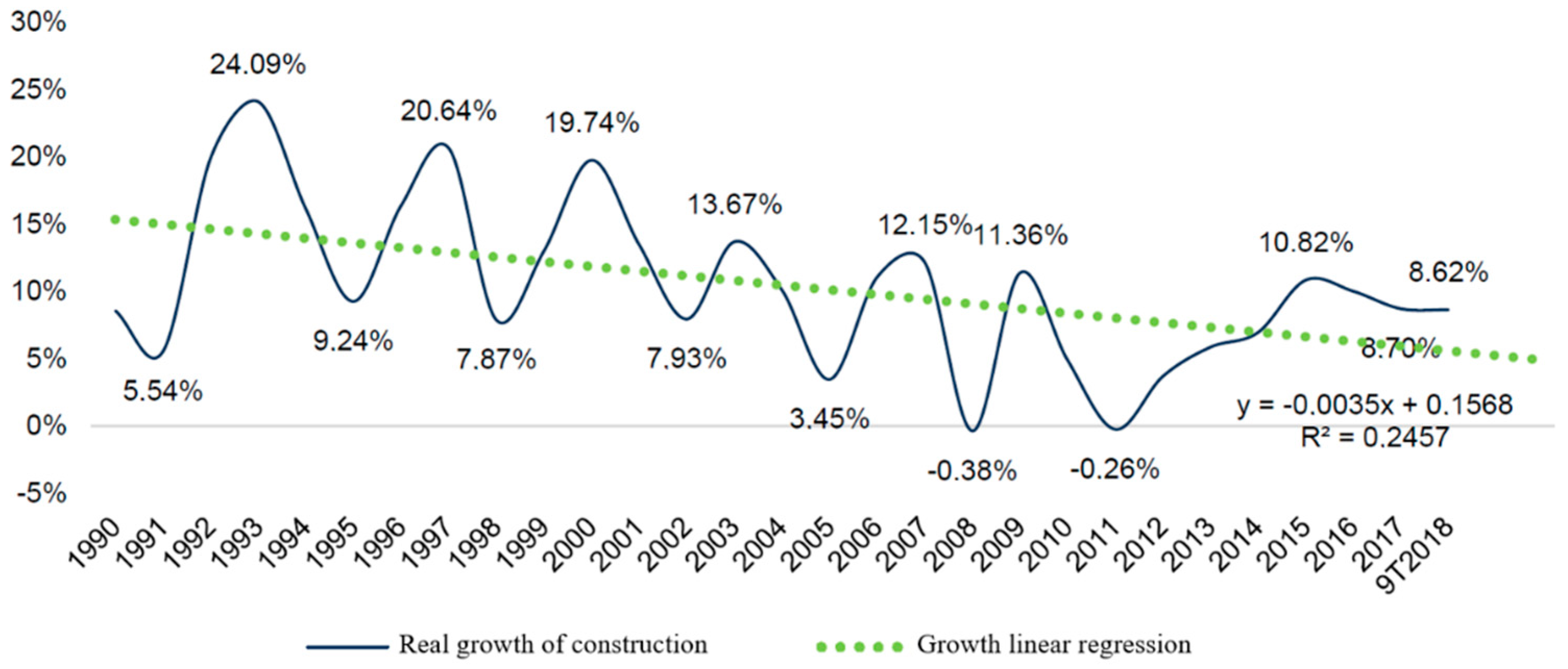
Accordingly, foreign-invested construction enterprises have the greatest competitive edge, followed by private enterprises, and state-owned ones [3]. As a whole, Vietnam’s construction industry in the period of 1990–2018 underwent six complete accelerating–decelerating cycles lasting about 4–5 years each, as demonstrated in Figure 2.
However, the business side of construction companies still faces many difficulties and challenges. As with other sectors, construction companies continue to suffer from economic difficulties. The infrastructure business in industrial zones is sluggish due to lack of investors. On the other hand, many industrial parks suffer from low occupancy. Huge debts are unresolved, especially in key projects, which have large capital scale and indirectly increase bad debt. Receivables of most enterprises lead to financial imbalances. Due to the lack of capital, the mobilization of capital sources in difficult situations enhances the negative impact on the production and business of enterprises in the construction industry. In addition, the transportation costs and input prices of raw materials and other supplies increased, while the selling price of products did not. This affected production and business efficiency.
Therefore, construction companies should find appropriate partners to deal with these issues by using the Grey model (GM (1,1)) to forecast business situations for the period of 2019–2022 [4]. Additionally, the super-slack-based measure (Super-SBM-I-V) model helps choose the most appropriate strategic combination in order to promote the strengths of each business and achieve goals. This model predicts future business and measures operation efficiency by using critical input and output variables. The autoregressive integrated moving average (ARIMA) model was used with data strings on the revenues of enterprises chosen to form alliances in the period 2009–2018 to determine future jobs and revenue trends of enterprises when carrying out the alliances [5]. These models were considered a prerequisite for the development of other activities in the construction industry to meet the goals of sustainable development. For the above reasons, integrating three models—the Super-SBM-I-V model, the GM (1,1) model, and the ARIMA model—in alliance decision-making is a new effective approach in this research.
The Grey system theory is an interdisciplinary scientific field, introduced in 1982 by Deng [6]. It is used to process, predict, and estimate the behavior of future data based on an initial range of constraints.
In the past, researchers worldwide used the data envelopment analysis (DEA) model to analyze and find strategic alliances in a variety of industries. Candace and contributors (2011) stated that strategic alliance is needed for innovation [7]. Kauser and Shaw (2004) further clarified the goals and motives of international strategic alliance by empirically studying strategic alliance agreements among the United Kingdom and Northern Ireland companies and their European, Japanese, and United States partners [8]. Chia-Nan Wang and Xuan-Tho Nguyen used the DEA and Grey theoretical models to analyze and select strategic partners in the automotive industry [9]. The results of this research possibly showed a strategic coalition in the automotive sector between Nissan and its partner, Renault. In addition, using the DEA and Grey method, Chia-Nan Wang and Han-Khanh Nguyen (2017) studied and found partnerships in textile enterprises in Vietnam [10]. According to the results of their research, textile enterprises should engage in strategic alliance to enhance their strengths and develop sustainably.
However, previous studies did not use a combination of multiple models to forecast the revenue of businesses after a union. Meanwhile, considering the development trend of employment, the revenue of businesses after a union is extremely important and helps managers decide whether to implement the alliance or not. In this study, the authors use the ARIMA model to solve this problem, offering managers a multi-dimensional perspective when making business decisions.
2. Research Development
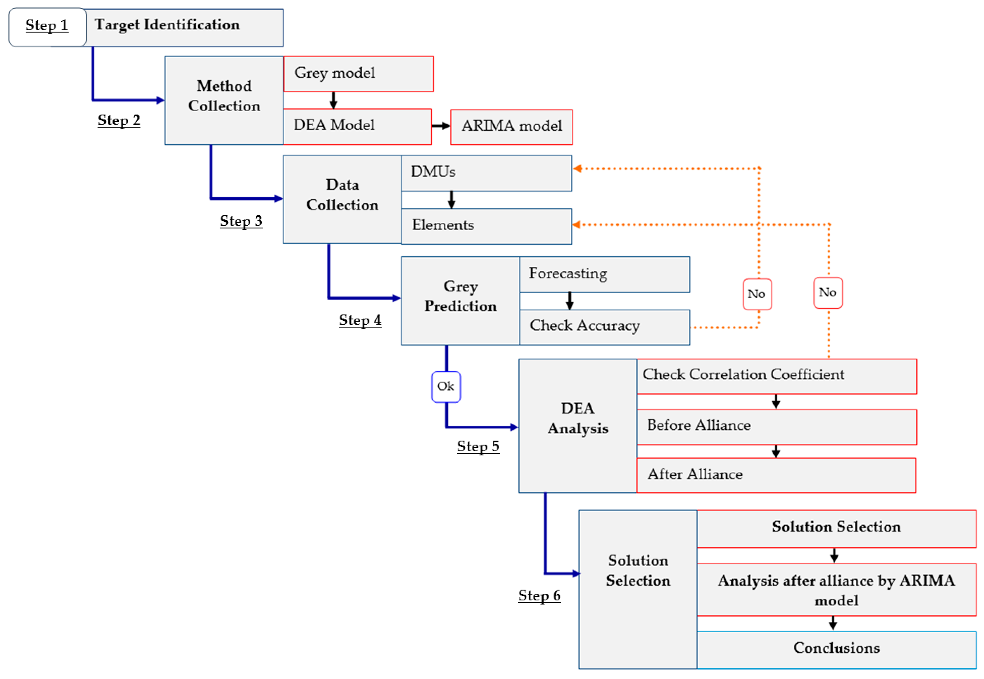
In this study, the GM (1,1) was used to predict the business results of the decision-making units (DMUs) for the 2019–2022 period; the Super-SBM-I-V model was used to select strategic partners for the construction companies; the ARIMA model was used to determine the jobs and revenue trends of enterprises in the future for forming the alliances. They are described below. This study used the following steps (Figure 3):
Step 1. Determining targets: according to current state of the construction industry, the labor, material, and equipment transportation costs are increasing. The authors find that the issues of costs and human resources need to be resolved to reduce prices, thereby giving construction enterprises in the Vietnamese market a competitive edge.
Step 2. Defining predictive methods: In this research, the authors concurrently employed several common models to analyze and assess the business efficiency of enterprises, which is described below.
The non-radial super efficiency model (Super–SBM) of DEA was used to assess the efficiency of the investment in technique and technology and the business efficiency of construction enterprises in Vietnam in the period 2015–2018. This result was the basis for the authors’ selection of strategic partners for the enterprises in the future.
The Grey forecasting model GM (1,1) was used to forecast all indicators used for the analysis in this research in order to forecast the business performance of construction enterprises in Vietnam for the period 2019–2022.
Each predictive method used in this research has its own pros and cons, depending on the statistical inputs and purpose of each model. The autoregressive integrated moving average model (ARIMA) was used by the authors as it is suitable for linear relationships among data in past, present, and future predictions [11]. This model was used in conjunction with the data strings on the revenues in the period 2009–2018 of the enterprises chosen to carry out the alliance to determine the jobs and revenue trends of the enterprise in the future when carrying out the alliance.
Step 3. Collecting data:
In this research, the authors collected the data from the website of the General Statistics Office of Vietnam.
Collecting the factors for analysis:
Input factors were as follows: total assets (TA); cost of goods sold (CS); total operating expense (TE); owners’ equity (OE).
Output factors were as follows: net sales (NS); profit after tax (PT).
Step 4. Grey prediction: The authors used the business data of the enterprises in the period 2015–2018 and used GM (1,1) to predict the business performance result for the period 2019–2022. Afterward, the authors used the mean absolute percentage error (MAPE) method to check the compatibility of the samples. If the error was not sufficiently reliable, the authors re-chose the sample enterprises.
Step 5. DEA analysis: Firstly, the authors used the Pearson coefficient to examine the correlation between the inputs and outputs in accordance with the requirements for using DEA. If the correlation coefficient was unsatisfactory, the authors repacked the components to ensure compatibility with the model. Afterward, the non-radial super efficiency model was used to compute, analyze, and assess the business performance of enterprises. From this result, the authors chose the target enterprise to carry out the alliance with other enterprises.
Step 6. Selecting solutions: After matching the target enterprise with 13 other enterprises, the authors used the result to select a suitable alliance solution for construction enterprises in Vietnam. After the appropriate alliance was chosen for the enterprises, the ARIMA model was used to determine the jobs and revenue trends of the enterprises in the future when carrying out the alliance. From such results, the authors provided the optimal evaluation and assessment of the chosen alliance for construction enterprises in Vietnam.
3. Research Method
3.1. Grey Forecasting Model
Values must fall within the range of
GM (1,1) is based on (a and b are coefficients).
Original data are from the following value chain:
X(0) = (x(0)(1), x(0)(2), …, x(0)(n)); n ≥ 4.
The original values that satisfy the above conditions are implemented in the following order:
Step 1. Use the cumulative plus method:
Step 2. Establish the GM (1,1) equation:
Step 3. Calculate the parameters a and b based on the least-squares method:
Step 4. Build the formula to calculate the predicted values as follows:
Find the GM (1,1) model’s predictive values using the following formula:
3.2. Non-Radial Super Efficiency Model (Super Slacks-Based Measure (SBM))
DEA is a powerful quantitative, analytical tool for measuring and evaluating performance. DEA was successfully applied to a host of different types of entities engaged across the industry sector. In DEA, there are several methods for measuring efficiency changes over time, in which DEA has two clusters: non-radial and radial. Non-radial models are based on the slacks-based measure (SBM) of efficiency. This SBM type model has nine variations. The first six, Super-SBM-I-C, Super-SBM-I-V, Super-SBM-I-GRS, Super-SBM-O-C, Super-SBM-O-V, and Super-SBM-O-GRS are “oriented”, while the other three, Super-SBM-C, Super-SBM-V, and Super-SBM-GRS, are “non-oriented”. In this research, the authors used the slacks-based measure of efficiency model to measure the business efficiency of the enterprises. The slacks-based measure of efficiency model was applied and developed by many researchers in various fields, which brought about good results [17,18,19,20,21]. Accordingly, the slacks-based measure of efficiency model was established according to the following equations:
Suppose (p*, λ*,) is the optimal condition of SBM, and is SBM efficient of DMU.
When p* = 1, (in fact, the inputs are irredundant, and the outputs change). Therefore, the researchers developed it into the super-efficiency model, as determined in accordance with the following formulas:
However, while the inputs are fixed, the outputs are still non-specific. To solve this issue, the researchers continued to use the DEA Solver Pro 4.1 Manual as follows:
Suppose . It defines as follows:
If there is no positive component in the output r, it becomes . The element becomes a replacement, while is unchanged.
When , the element is
When , the element becomes
3.3. Autoregressive Integrated Moving Average Model (ARIMA)
The ARIMA model was introduced by Box and Jenkins in 1970 [22]. The ARIMA model consists of three main components: (1) AR (autoregression component); (2) I (stationarity of time series); (3) MA (moving averages component). The steps of applying the ARIMA conjecturing model are as follows [23,24,25,26,27]:
Step 1. Identify the three p, d, and q components of the ARIMA model.
The authors used the augmented Dickey–Fuller unit root test and the Phillips–Perron test to test the stationarity of the series.
The autoregression model of order p, notated as AR(p), is defined as
is the time series, while is the expected value of , and is white noise.
The moving average model of order q in the MA(q) model is calculated as follows:
Combining Equations (18) and (19), we have the ARIMA(p,q) model as follows:
We then calculate the appropriate p, d, q values in the ARIMA model, in which, p and q depend on the PACF = f(t) and ACF = f(t) graphs.
Step 2. Estimate the parameters and select the model using Statistical Package for the Social Sciences software.
Step 3. Check the model: The research used the mean absolute percent error (MAPE) index to assess the reliability of the conjecturing model.
Step 4. Conjecturing: After the errors of the conjecturing models were checked, the models were used to conjecture the trends for the enterprises if they were suitable.
3.4. Evaluation of Volatility Forecasts
To test the accuracy of the predicted values, the authors used MAPE, which is a popular and reliable tool for measuring accurate values in statistics. When MAPE is smaller, the predicted value is closer to the actual value [28,29].
MAPE is divided into four ranks, as shown in Table 1.
3.5. Materials and Methods
3.5.1. DMU Collection
In order to meet the requirements of the Grey theory and DEA models used in this study, DMUs (decision-making units) must meet the following mandatory requirements in terms of scale and time of operation: business data must be accurate, specific, and clear. After finding DMUs from the General Statistics Office’s website in the construction industry in Vietnam, we collected 14 suitable DMUs, as shown in Table 2.
3.5.2. Input/Output Collection
Because the inputs/outputs have a direct impact on the results of the analysis and evaluation of the study, we carefully selected four inputs and two outputs from the financial statement of the DMUs.
The input factors were as follows:
Total assets (TA) reflect all tangible and intangible assets of the business;
Owners’ equity (OE) is the capital owned by the business owner;
Cost of goods sold (CS) is one of the costs that account for a large proportion of the production process;
Total operating expenses (TE) reflect the total daily cost of sales and management or research and development.
The output factors were as follows:
Net sales (NS) reflects the turnover of selling goods and providing service of enterprises;
Profit after tax (PT) reflects the business results (profit and loss) after income tax.
The above factors reflect the overall business situation of the enterprises (assets, costs, and profits). These factors are a highly reliable and sufficient basis for analysis, calculation, and evaluation in the study. The authors summarized the data of enterprises in the period of 2015–2018, calculated according to each year, in Table 3, Table 4, Table 5, Table 6 and Table 7.
4. Results
4.1. Results and Analysis of the Grey Forecasting
We used GM (1,1) to predict the business performance of DMUs in the 2019–2022 period. The predicted data were calculated as outlined below (we use total assets of DMU8 in Table 7 to explain this process).
The base range is the actual data for the 2015–2018 periods as follows:
X(0) = (602210; 693526; 860951; 972467).
Using the accumulated generating operation (AGO) method, we obtain the following:
The GM (1,1) equation is established as follows:
To find the coefficients of a and b, the initial values are placed in the following system of equations:
The above equation is converted into a matrix as follows:
The least-squares method is used to find a and b as follows:
The two coefficients a and b are used to generate the whitening equation of the differential equation as follows:
The predicted values are calculated using the following formula:
In turn, the values of k are replaced as follows:
| k = 0; | = 602,210; |
| k = 1; | = 1,309,482.399; |
| k = 2; | = 2,142,296.171; |
| k = 3; | = 3,122,935.003; |
| k = 4; | = 4,277,637.952; |
| k = 5; | = 5,637,301.527; |
| k = 6; | = 7,238,306.391; |
| k = 7; | = 9,123,490.801. |
Using the accumulated generating operation (AGO) method to compute the predicted values based on the original data, we obtain the following results:
Similarly, we can obtain the forecast value of the enterprises in the 2019–2022 period, as shown in Table 8, Table 9, Table 10 and Table 11.
To verify the accuracy of the predicted values to ensure an appropriate predictive method, we used MAPE. The results are shown in Table 12.
As shown in the above result, there were 11 DMUs with MAPE <10% (the average MAPE of 14 DMUs was 6.50%). According to the convention in Table 6, the predictive values in this study had high accuracy. This shows that GM (1,1) used in this study is consistent, predictive, and highly reliable.
4.2. Pearson Correlation
We used the Super-SBM-I-V model to find strategic alliance partners for the businesses. To ensure suitability when using DEA, we used the Pearson coefficient to determine the appropriate correlation between the factors (i.e., the correlative coefficient between non-negative or zero elements; if this coefficient is close to 1, the linear relationship between those two elements is stronger). Results are shown in Table 13, Table 14, Table 15 and Table 16.
The results shown from Table 13, Table 14, Table 15 and Table 16 demonstrate that the inputs and the outputs in this research have strong correlation, which satisfies the requirements of the DEA. These factors were used to evaluate the business results of construction enterprises in order to find the most suitable strategic allies.
4.3. Analysis Alliance
4.3.1. Analysis before Alliance
Based on the data on the actual business performance of the enterprises in 2018, we used the Super SBM-I-V model of the DEA to assess the business performance of the enterprises. Based on this result, we chose the target enterprises to ally with other enterprises. The results are provided in Table 17.
4.3.2. Analysis after Alliance
Based on the results of business performance analysis and business rankings derived from the Super-SBM-I-V software in Table 17, we established DMU12 as the alliance target for the enterprise. When choosing DMU4, DMU13, or DMU11, it would be difficult to persuade other DMU alliances when their business situation is too low. When combining DMU12 with the 13 other DMUs, we found 27 coordinates. Using the DEA-Solver Pro 8.0-Super-SBM-I-V model to evaluate the business performance of these 27 combinations, we obtained the results shown in Table 18.
From the results of the analysis, we chose DMU12 as a target company to combine with other companies because the results of DMU12’s business in 2018 were ineffective (rank DMU12 = 11 (11/14 DMUs); score DMU12 = 0.7946). In that situation, the DMU12 leaders needed to have practical solutions to change and improve the business situation. The solution of combining with other enterprises is a feasible new direction. On the other hand, DMU12 (Vietnam Construction Joint Stock Company No. 2) in Hanoi is one of the leading companies in the construction industry. Hanoi consists of good roads, railways, waterways, and air and sea transport systems. It is convenient for other businesses to choose DMU12 as a partner for the alliance.
Based on the results of assessing the business performance of the enterprises when joining the alliance, we divided them into two groups, as outlined below.
Group 1 (Table 19) includes effective alliances.
These alliances can encourage managers to consider possible implementation in the future, as these alliances work well for all parties involved. In particular, before implementing the DMU12 alliance, ranked 11/14, the effective score was only 0.7946. However, after making a coalition with DMU8, the situation of the business improved significantly (rank 6/27, efficiency score 1.1977). This union would help both DMU8 and DMU12 to operate effectively.
Group 2 (Table 20) includes ineffective alliances.
Alliances that would not work well should not be encouraged in the future.
4.3.3. Partner Alliance Selection
Based on the results of the assessment in Table 19, the proposal for the implementation of the alliance (DMU12 + DMU8) was the best solution for all parties.
VC2 (Vietnam Construction Joint Stock Company No.2) was established in 1970, and it specializes in constructing and building civil works, industrial works, road transportation at all levels, bridges, irrigation works, posts, foundations, urban and industrial technical infrastructure works, lines, transformers, and water supply and drainage works, as well as installing technology pipeline and pressure, electrical works, etc.
THG (Tien Giang Investment and Construction Joint Stock Company) is the precursor of Tien Giang Investment and Construction Joint Stock Company. THG’s board of directors is planning a strategy to promote its strength in irrigation construction, allying with strategic partners to expand to construction, industrial construction, and environment projects to strengthen its position, as well as increase revenue and profits.
Therefore, considering the fields of business and the strategies, this alliance can achieve positive results and expand the markets for all enterprises. When the alliance is established, the parties can develop policies to diversify possible products. In addition, the alliance will also have more customers by taking advantage of their different customer systems. If there are works in appropriate and advantageous locations for their allies, the parties can use the machinery, raw materials, and common labor of their allies in the location. This will assist in keeping production stabilized and timely, which in turn will reduce construction and transportation time, as well as production and workers living costs. As a result, this will help strengthen the enterprise’s position and competitive edge in the market, thereby increasing business efficiency.
4.3.4. Analysis after Alliance by ARIMA Model
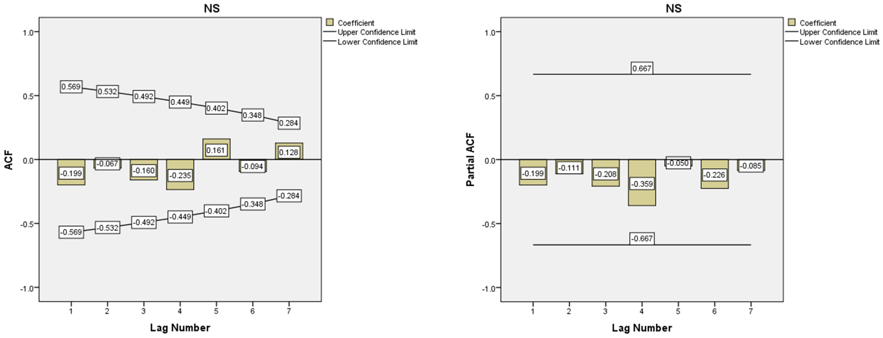
To ensure suitability when using the ARIMA model, we firstly examined the stationarity of the time series with respect to the revenue in the period 2009–2018 of the enterprises in the alliance. The result shows that the time series were non-stationary at a zero-degree difference; therefore, a first-degree difference was used to examine stationarity. After a first-degree difference was used, the time series were stationary (Figure 4).
Then, the authors used the experimental method of comparing the R2-squared indexes to come up with a suitable conjecturing model. The comparison shows that the ARIMA (1,1,1) model is the most suitable model for the dataset with respect to the revenue in the period 2009–2018 (Figure 5).
We continued to examine the suitability of the model by calculating the MAPE index of the ARIMA(1,1,1) model. The result in Table 21 shows that the model used in this research has high accuracy with MAPE = 19.642% (Sig. = 0.00).
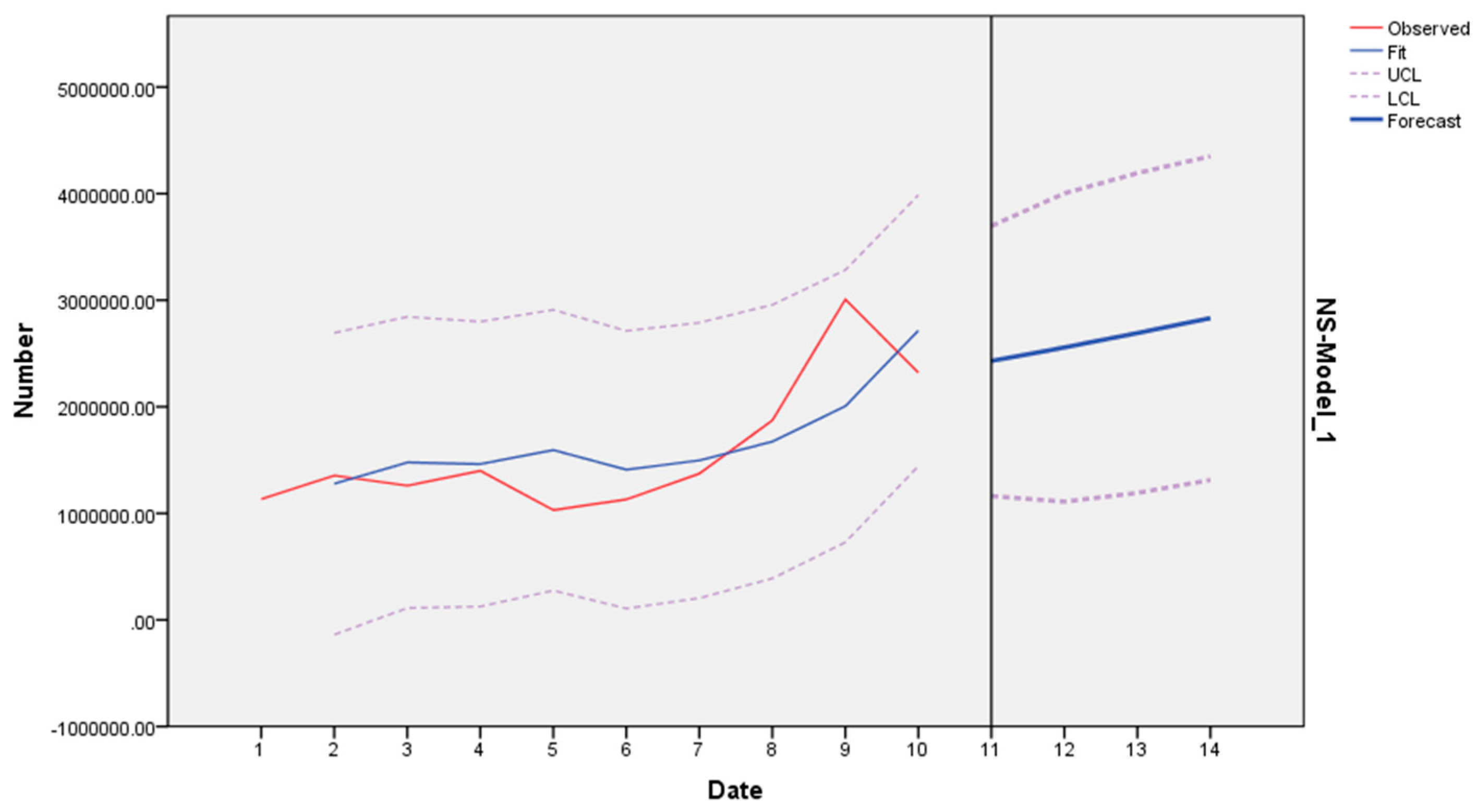
The prediction result by the ARIMA model in Table 22 and Figure 6 shows that the revenue trend would be upward throughout the years following enterprise alliance. Specifically, when DMU8 makes an alliance with DMU12, the forecasted revenue for the years from 2019 to 2020 would be as follows: 2,429,442.05; 2,556,578.22; 2,692,219.24; 2,831,908.40. This means that, if they ally, they would have more contracts from bidding and build more civil and industrial construction work.
Therefore, the conjectured result from the ARIMA model can help corporate managers and policy-makers put forward plans to deal with fierce competition in the future, as well as open up the opportunity for cooperation, promotion, and market expansion for enterprises. In addition, this research result allows corporate managers of construction enterprises to use the conjectured result in putting forward business plans to ensure a good implementation of their enterprise strategies.
5. Discussion and Conclusions
Currently, the competition among enterprises in the market is extremely fierce, and enterprises may become bankrupt if they do not have sufficient financial and technological capacity. Therefore, the alliance between enterprises can help them sharpen their competitive edge compared to other competitors. In this research, we used the DEA and GM (1,1) models to choose an appropriate strategic partner for a construction enterprise. Furthermore, the ARIMA model showed that, if the alliance is conducted, the revenue trend of the enterprises would increase, meaning that they would have more design and construction contracts. Therefore, the proposed solution can help companies assist each other, as well as cooperate and make use of existing resources related to investment, technology, techniques, and unskilled labor to design and build construction works.
In this study, we used the business data of the top 14 enterprises in construction investment, responsible for designing and executing the work for civil and industrial projects in Vietnam from 2015 to 2018. We used DEA models to evaluate the business performance of these businesses during the period of research, while we also used Grey system theory to forecast the business situation of companies for the period 2019–2022. Based on these results, we proposed alliances to benefit businesses in developing their own strengths and minimizing difficulties when the economy has many fluctuations, such as today. Then, we used the ARIMA model to predict the revenue trends of businesses when implementing the alliance. The use of multiple models which were considered and evaluated in this study can provide managers with a multi-dimensional and objective perspective to make decisions for businesses. The results of this study can help leading enterprises in the field of construction investment to have an appropriate coalition strategy in the context of a changing economy both in Vietnam and around the world. Regulatory authorities may use the results of this research to propose orientations, make decisions, and plan appropriate strategies to develop Vietnam’s construction industry.
In addition to these important contributions, this research still has certain limitations. Specifically, the authors only analyzed, evaluated, and forecasted business results based on quantitative data but without an in-depth analysis of factors on business environment and legal factors. Therefore, in the future, research should be carried out in combination with environmental factors and regulations and policies of state management in the field of construction in order to have better solutions to provide managers with a better overview to plan strategies and make more accurate decisions.
Funding
This research received no external funding.
Conflicts of Interest
The authors declare no conflict of interest.
References
- Thanh, D. Urbanization Rate in 2019 Will Reach 40%. Available online: http://kinhtedothi.vn/ (accessed on 1 April 2020).
- Hoa Khoa. What Are the Prospects for the Construction Industry in 2019? Available online: https://nhadautu.vn/ (accessed on 1 April 2020).
- Duy, N. Construction Industry Continues to Slow Down in 2019. Available online: https://cungcau.vn/ (accessed on 1 April 2020).
- Deng, J.-L. Introduction to Grey system theory. J. Grey Syst. 1989, 1, 1–24. [Google Scholar]
- Ho, S.-L.; Xie, M. The use of ARIMA models for reliability forecasting and analysis. Comput. Ind. Eng. 1998, 35, 213–216. [Google Scholar] [CrossRef]
- Candace, E.-Y.; Thomas, A.-T. Strategic alliances with competing firms and shareholder value. J. Manag. Mark. Res. 2011, 6, 1. [Google Scholar]
- Kauser, S.; Shaw, V. International strategic alliances: Objectives, motives and success. J. Glob. Mark. 2004, 17, 7–43. [Google Scholar] [CrossRef]
- Wang, C.-N.; Nguyen, X.; Wang, Y. Automobile Industry Strategic Alliance Partner Selection: The Application of a Hybrid DEA and Grey Theory Model. Sustainability 2016, 8, 173. [Google Scholar] [CrossRef] [Green Version]
- Wang, C.N.; Nguyen, H.K.; Liao, R.Y. Partner Selection in Supply Chain of Vietnam’s Textile and Apparel Industry: The Application of a Hybrid DEA and GM (1,1) Approach. Math. Probl. Eng. 2017. [Google Scholar] [CrossRef] [Green Version]
- Statistics. General Statistics Office of Vietnam. Available online: https://www.gso.gov.vn (accessed on 25 October 2019).
- Kumar, M.; Anand, M. An Application of Time Series Arima Forecasting Model for Predicting Sugarcane Production in India. Stud. Bus. Econ. 2014, 9, 81–94. [Google Scholar]
- Kayacan, E.; Ulutas, B.; Kaynak, O. Grey system theory-based models in time series prediction. Expert Syst. Appl. 2010, 37, 1784–1789. [Google Scholar] [CrossRef]
- Deng, J. Control problems of grey systems. Syst. Control Lett. 1982, 1, 288–294. [Google Scholar]
- Yin, M. Fifteen years of grey system theory research: A historical review and bibliometric analysis. Expert Syst. Appl. 2013, 40, 2767–2775. [Google Scholar] [CrossRef]
- Li, G.-D.S.; Masuda, S.; Nagai, M. An Optimal Prediction Model using Taylor Approximation Method. J. Grey Syst. 2011, 11, 173. [Google Scholar] [CrossRef]
- Liu, S.-F.; Forrest, J. The current development status on grey system theory. J. Grey Syst. 2007, 19, 111–123. [Google Scholar]
- Miliotis, P.A. Data envelopment analysis applied to electricity distribution districts. J. Oper. Res. Soc. 1992, 43, 549–555. [Google Scholar] [CrossRef]
- Banker, A.; Charnes, W.; Cooper, W. Some models for estimating technical and scale efficiencies in data envelopment analysis. Manag. Sci. 1984, 30, 1078–1092. [Google Scholar] [CrossRef] [Green Version]
- Tone, K. A slacks-based measure of super-efficiency in data envelopment analysis. Eur. J. Oper. Res. 2002, 143, 32–41. [Google Scholar] [CrossRef] [Green Version]
- Charnes, W.; Cooper, W.; Rhodes, E. Measuring the efficiency of decision making units. Eur. J. Oper. Res. 1978, 2, 429–444. [Google Scholar] [CrossRef]
- Azadeh, A.; Ghaderi, S.F.; Javaheri, Z.; Saberi, M. A fuzzy mathematical programming approach to DEA models. Am. J. Appl. Sci. 2008, 5, 1352–1357. [Google Scholar] [CrossRef] [Green Version]
- Box, G.; Jenkin, G. Time Series Analysis, Forecasting and Control; Holden-Day: San Francisco, CA, USA, 1970; pp. 234–239. [Google Scholar]
- Stellwagen, E.; Tashman, L. Arima: The Models of Box and Jenkins. Foresight. Int. J. Appl. Forecast. 2013, 30, 28–33. [Google Scholar]
- Dickey, D.; Fuller, W. Distribution of the Estimators for Autoregressive Time Series with a Unit Root. J. Am. Stat. Assoc. 1979, 74, 427–431. [Google Scholar]
- Brockwell, P.J.; Davis, R.A. Introduction to Time Series and Forecasting; Springer: New York, NY, USA, 2001; pp. 180–196. [Google Scholar]
- Cummins, D.; Griepentrog, G. Forecasting automobile insurance paid claim costs using econometric and ARIMA models. Int. J. Forecast. 1985, 1, 203–215. [Google Scholar] [CrossRef]
- Ediger, V.S.; Akar, S. ARIMA forecasting of primary energy demand by fuel in Turkey. Energy Policy 2007, 35, 1701–1708. [Google Scholar] [CrossRef]
- Yu, M.; Wang, C.; Ho, N. A Grey Forecasting Approach for the Sustainability Performance of Logistics Companies. Sustainability 2016, 8, 866. [Google Scholar] [CrossRef] [Green Version]
- Wang, C.-N.; Nguyen, H.-K. Enhancing Urban Development Quality Based on the Results of Appraising Efficient Performance of Investors—A Case Study in Vietnam. Sustainability 2017, 9, 1397. [Google Scholar] [CrossRef] [Green Version]
- McKenzie, J. Mean absolute percentage error and bias in economic forecasting. Econ. Lett. 2011, 113, 259–262. [Google Scholar] [CrossRef]
Figure 1.
Volatility in construction industry index and Vietnam index [2].
Figure 1.
Volatility in construction industry index and Vietnam index [2].

Figure 2.
Real growth of Vietnam’s construction industry (1990–2018) [3].
Figure 2.
Real growth of Vietnam’s construction industry (1990–2018) [3].

Figure 3.
Research process.

Figure 4.
The time series were stationary after implementation of first-degree difference.

Figure 5.
Upper and lower confidence limits of coefficient.

Figure 6.
Forecast revenue trend after alliance.


Table 1.
The grades of mean absolute percent error (MAPE).
| MAPE Valuation (%) | 10 | 10–20 | 20–50 | 50 |
|---|---|---|---|---|
| Accuracy | Excellent | Good | Qualified | Unqualified |
Source: Reference [30].
Table 2.
List of companies [10]. DMU—decision-making unit.
Table 2.
List of companies [10]. DMU—decision-making unit.
| DMUs | Code | DMUs | Code |
|---|---|---|---|
| DMU1 | HU3 JSC | DMU8 | THG JSC |
| DMU2 | C32 JSC | DMU9 | HU6 JSC |
| DMU3 | CTD JSC | DMU10 | TV2 JSC |
| DMU4 | HU1 JSC | DMU11 | VC1 JSC |
| DMU5 | DXG JSC | DMU12 | VC2 JSC |
| DMU6 | HU4 JSC | DMU13 | VC3 JSC |
| DMU7 | SC5 JSC | DMU14 | VC9 JSC |
Table 3.
Data in 2015 (in million Vietnamese dong (VND)) [10]. TA—total assets; OE—owners’ equity; CS—cost of goods sold; TE—total operating expenses; NS—net sales; PT—profit after tax.
Table 3.
Data in 2015 (in million Vietnamese dong (VND)) [10]. TA—total assets; OE—owners’ equity; CS—cost of goods sold; TE—total operating expenses; NS—net sales; PT—profit after tax.
| DMUs | Inputs | Outputs | ||||
|---|---|---|---|---|---|---|
| (I)TA | (I)OE | (I)CS | (I)TE | (O)NS | (O)PT | |
| DMU1 | 620,161 | 177,678 | 371,279 | 38,010 | 426,554 | 16,468 |
| DMU2 | 445,496 | 325,687 | 413,001 | 24,658 | 557,407 | 101,287 |
| DMU3 | 7,815,096 | 3,242,536 | 12,557,080 | 364,408 | 13,668,916 | 799,525 |
| DMU4 | 632,857 | 179,595 | 595,002 | 27,063 | 629,294 | 8634 |
| DMU5 | 3,573,347 | 1,771,359 | 735,260 | 277,948 | 1,394,505 | 554,605 |
| DMU6 | 738,418 | 244,283 | 172,733 | 23,791 | 195,091 | 6506 |
| DMU7 | 2,254,213 | 311,234 | 1,358,256 | 42,690 | 1,431,205 | 35,771 |
| DMU8 | 602,210 | 204,906 | 549,159 | 91,770 | 699,471 | 56,077 |
| DMU9 | 171,734 | 93,210 | 26,023 | 16,926 | 54,412 | 9947 |
| DMU10 | 1,666,729 | 605,067 | 320,629 | 34,472 | 416,693 | 63,352 |
| DMU11 | 578,886 | 240,065 | 342,574 | 14,625 | 367,520 | 11,945 |
| DMU12 | 1,564,386 | 276,713 | 604,079 | 52,074 | 673,198 | 14,826 |
| DMU13 | 1,232,421 | 242,305 | 390,277 | 41,837 | 477,037 | 42,965 |
| DMU14 | 1,335,468 | 190,956 | 695,206 | 54,678 | 755,093 | 11,077 |
Table 4.
Data in 2016 (in million VND) [10].
Table 4.
Data in 2016 (in million VND) [10].
| DMUs | Inputs | Outputs | ||||
|---|---|---|---|---|---|---|
| (I)TA | (I)OE | (I)CS | (I)TE | (O)NS | (O)PT | |
| DMU1 | 610,046 | 181,458 | 501,990 | 34,613 | 557,289 | 16,723 |
| DMU2 | 552,905 | 380,276 | 382,480 | 35,357 | 520,269 | 93,327 |
| DMU3 | 1,1740,871 | 6,233,628 | 18,983,319 | 299,422 | 20,782,721 | 1,422,144 |
| DMU4 | 653,954 | 175,646 | 361,757 | 17,949 | 385,414 | 2968 |
| DMU5 | 5,562,791 | 3,537,355 | 1,454,880 | 441255 | 2,506,517 | 791,643 |
| DMU6 | 986,077 | 251,440 | 267,696 | 26,183 | 303,203 | 13,540 |
| DMU7 | 1,987,448 | 319,615 | 1,389,419 | 40,714 | 1,471,018 | 41,926 |
| DMU8 | 693,526 | 275,639 | 643,742 | 92,720 | 829,611 | 86,648 |
| DMU9 | 179,954 | 95,298 | 50,566 | 14,510 | 76,009 | 10,884 |
| DMU10 | 1,998,479 | 653,337 | 420,233 | 15,613 | 476,012 | 37,770 |
| DMU11 | 799,291 | 238,715 | 514,582 | 28,469 | 555,272 | 12,843 |
| DMU12 | 2,539,223 | 292,291 | 899,563 | 69,822 | 1,043,090 | 30,878 |
| DMU13 | 1,157,266 | 299,950 | 433,356 | 33,295 | 557,042 | 75,352 |
| DMU14 | 1,375,140 | 191,411 | 790,342 | 53,792 | 848,714 | 13,877 |
Table 5.
Data in 2017 (in million VND) [10].
Table 5.
Data in 2017 (in million VND) [10].
| DMUs | Inputs | Outputs | ||||
|---|---|---|---|---|---|---|
| (I)TA | (I)OE | (I)CS | (I)TE | (O)NS | (O)PT | |
| DMU1 | 742,475 | 195,429 | 330,224 | 43,297 | 393,984 | 19,685 |
| DMU2 | 747,661 | 439,990 | 418,738 | 39,100 | 559,746 | 91,653 |
| DMU3 | 15,877,318 | 7,306,688 | 25,137,241 | 394,619 | 27,176,837 | 1,652,679 |
| DMU4 | 966,959 | 174,063 | 504,847 | 25,526 | 542,399 | 4645 |
| DMU5 | 10,264,403 | 4,653,845 | 1,149,440 | 606,189 | 2,879,241 | 1,419,950 |
| DMU6 | 701,752 | 248,757 | 259,228 | 19,267 | 289,973 | 9056 |
| DMU7 | 2,013,640 | 345,438 | 1,849,664 | 85,329 | 1,967,025 | 59,982 |
| DMU8 | 860,951 | 321,664 | 683,568 | 125,279 | 909,854 | 90,803 |
| DMU9 | 151,125 | 95,692 | 55,862 | 15,493 | 80,900 | 8485 |
| DMU10 | 2,191,711 | 698,002 | 524,721 | 49,300 | 637,466 | 64,227 |
| DMU11 | 813,115 | 240,134 | 560,231 | 51,619 | 623,227 | 15,176 |
| DMU12 | 2,259,759 | 305,715 | 1,860,963 | 159,349 | 2,096,871 | 31,406 |
| DMU13 | 785,519 | 332,441 | 457,728 | 38,680 | 542,239 | 43,506 |
| DMU14 | 1,684,956 | 190,531 | 991,995 | 51,492 | 1,063,354 | 12,608 |
Table 6.
Data in 2018 (in million VND) [10].
Table 6.
Data in 2018 (in million VND) [10].
| DMUs | Inputs | Outputs | ||||
|---|---|---|---|---|---|---|
| (I)TA | (I)OE | (I)CS | (I)TE | (O)NS | (O)PT | |
| DMU1 | 744,126 | 168,295 | 560,514 | 42,859 | 627,430 | 21,363 |
| DMU2 | 782,679 | 491,588 | 552,524 | 67,430 | 722,333 | 92,446 |
| DMU3 | 16,823,062 | 7,962,493 | 26,727,845 | 505,474 | 28,560,857 | 1,515,408 |
| DMU4 | 953,267 | 165,729 | 445,947 | 40,437 | 496,346 | 8595 |
| DMU5 | 13,728,715 | 6,199,094 | 2,030,544 | 970,488 | 4,645,319 | 2,267,163 |
| DMU6 | 582,109 | 198,610 | 144,269 | 12,820 | 165,349 | 3381 |
| DMU7 | 1,916,641 | 349,156 | 2,497,980 | 51,032 | 2,596,707 | 39,684 |
| DMU8 | 972,467 | 349,366 | 730,035 | 138,058 | 956,687 | 80,354 |
| DMU9 | 155,853 | 88,719 | 9066 | 17,008 | 35,502 | 9680 |
| DMU10 | 2,192,694 | 698,983 | 1,474,988 | 127,566 | 1,840,415 | 225,105 |
| DMU11 | 885,562 | 238,765 | 461,133 | 53,868 | 501,708 | 15,807 |
| DMU12 | 2,282,518 | 303,394 | 1,228,574 | 108,685 | 1,363,487 | 24,038 |
| DMU13 | 843,835 | 383,562 | 234,507 | 35,528 | 290,305 | 22,787 |
| DMU14 | 1,570,296 | 184,214 | 1,339,947 | 59,571 | 1,384,872 | 8152 |
Table 7.
Data of DMU8 from 2015 to 2018 (in million VND).
| Year | Inputs | Outputs | ||||
|---|---|---|---|---|---|---|
| (I)TA | (I)OE | (I)CS | (I)TE | (O)NS | (O)PT | |
| 2015 | 602,210 | 204,906 | 549,159 | 91,770 | 699,471 | 56,077 |
| 2016 | 693,526 | 275,639 | 643,742 | 92,720 | 829,611 | 86,648 |
| 2017 | 860,951 | 321,664 | 683,568 | 125,279 | 909,854 | 90,803 |
| 2018 | 972,467 | 349,366 | 730,035 | 138,058 | 956,687 | 80,354 |
Sources: Collected by researcher [10].
Table 8.
Data in 2019 (in million VND).
| DMUs | Inputs | Outputs | ||||
|---|---|---|---|---|---|---|
| (I)TA | (I)OE | (I)CS | (I)TE | (O)NS | (O)PT | |
| DMU1 | 838,708.92 | 169,400.37 | 535,903.13 | 48,839.72 | 610,615.71 | 24,286.45 |
| DMU2 | 944,641.58 | 559,548.14 | 654,438.07 | 91,456.08 | 838,388.03 | 91,593.75 |
| DMU3 | 20,386,203.04 | 9,044,473.61 | 32,093,863.81 | 650,102.90 | 339,46913.15 | 1,621,838.81 |
| DMU4 | 1,177,887.82 | 162,183.59 | 521,392.58 | 58,801.25 | 587,549.95 | 13,702.14 |
| DMU5 | 20,538,708.63 | 8,098,952.01 | 2,302,395.13 | 1,398,279.30 | 6,213,266.41 | 3,589,967.93 |
| DMU6 | 423,473.25 | 186,253.03 | 131,746.90 | 9383.82 | 149,351.13 | 2558.77 |
| DMU7 | 1,903,487.71 | 368,301.52 | 3,300,602.61 | 67,908.02 | 3,404,956.25 | 45,264.84 |
| DMU8 | 1,154,702.95 | 395,374.97 | 776,552.54 | 169,504.38 | 1,032,111.01 | 79,989.01 |
| DMU9 | 138,840.44 | 86,922.12 | 15,615.18 | 18,342.79 | 36,031.38 | 8466.04 |
| DMU10 | 2,325,846.83 | 729,796.26 | 2,290,102.19 | 259,478.27 | 2,853,432.09 | 294,582,81 |
| DMU11 | 923,571.18 | 239,254.57 | 462,997.05 | 73,546.81 | 511,242.15 | 17,749.81 |
| DMU12 | 2,109,580.93 | 311,633.92 | 1,626,628.32 | 148,664.52 | 1,787,202.62 | 22,821,13 |
| DMU13 | 636,219.23 | 431,402.81 | 229,348.37 | 38,033.29 | 267,258.20 | 13,657.43 |
| DMU14 | 1,739,166.58 | 181,663.63 | 1,722,528.71 | 61,170.85 | 1,750,642.10 | 7061.55 |
Sources: Calculated by researcher.
Table 9.
Data in 2020 (in million VND).
| DMUs | Inputs | Outputs | ||||
|---|---|---|---|---|---|---|
| (I)TA | (I)OE | (I)CS | (I)TE | (O)NS | (O)PT | |
| DMU1 | 920,388.73 | 163,592.73 | 576,597.29 | 53,899.36 | 658,731.09 | 27,355.68 |
| DMU2 | 1,107,361.86 | 635,138.19 | 795,181.01 | 131,959.31 | 997,366.88 | 91,156.55 |
| DMU3 | 24,046,944.07 | 10,190,457.85 | 37,604,817.24 | 841,388.44 | 39,335,282.20 | 1670,044.04 |
| DMU4 | 1,387,056.51 | 157,599.83 | 570,011.21 | 88,986.48 | 655,095.89 | 23,655.38 |
| DMU5 | 30,648,721.83 | 10,713,923.29 | 2,845,969.24 | 2,102,832.46 | 8,730,537.55 | 5,895,976.32 |
| DMU6 | 321,592.67 | 166,929.98 | 102,225.25 | 6,665.80 | 116,060.35 | 1464.87 |
| DMU7 | 1,869,976.43 | 384,565.29 | 4,422,365.07 | 72,884.54 | 4,510,032.97 | 44,331.58 |
| DMU8 | 1,359,663.58 | 443,812.74 | 827,046.52 | 204,002.94 | 1,107,205.95 | 77,191.40 |
| DMU9 | 128,572.45 | 83,947.77 | 10,188.93 | 19,872.79 | 27,335.22 | 7,923.89 |
| DMU10 | 2,432,788.32 | 754,310.21 | 4,861,631.62 | 649,432.98 | 6,318,919.13 | 793,845.02 |
| DMU11 | 973,262.66 | 239,279.53 | 440,499.21 | 95,558.97 | 488,636.45 | 19,605.23 |
| DMU12 | 1,995,608.51 | 317,394.22 | 1,801,587.19 | 171,235.15 | 1,952,098.64 | 20,373.04 |
| DMU13 | 530,320.47 | 488,564.30 | 180,982.47 | 39,189.76 | 205,415.87 | 7769.89 |
| DMU14 | 1,847,449.12 | 178,248.83 | 2,253,604.97 | 64,581.99 | 2,240,448.59 | 5578.47 |
Sources: Calculated by researcher.
Table 10.
Data in 2021 (in million VND).
| DMUs | Inputs | Outputs | ||||
|---|---|---|---|---|---|---|
| (I)TA | (I)OE | (I)CS | (I)TE | (O)NS | (O)PT | |
| DMU1 | 1,010,023.14 | 157,984.19 | 620,381.59 | 59,483.15 | 710,637.88 | 30,812.79 |
| DMU2 | 1,298,111.71 | 720,939.79 | 966,192.02 | 190,400.23 | 1,186,492.00 | 90,721.43 |
| DMU3 | 28,365,042.67 | 11,481,644.55 | 44,062,076.43 | 1,088,957.62 | 45,578,943.18 | 1,719,682.06 |
| DMU4 | 1,633,369.27 | 153,145.62 | 623,163.42 | 134,667.09 | 730,407.04 | 40,838.63 |
| DMU5 | 45,735,307.28 | 14,173,210.57 | 3,517,876.16 | 3,162,389.90 | 12,267,667.43 | 9,683,244.39 |
| DMU6 | 244,222.84 | 149,611.63 | 79,318.77 | 4735.06 | 90,190.18 | 838.62 |
| DMU7 | 1,837,055.13 | 401,547.25 | 5,925,376.41 | 782,25.75 | 5,973,761.74 | 43,417.57 |
| DMU8 | 1,601,004.86 | 498,184.66 | 880,823.79 | 245,522.85 | 1,187,764.70 | 74,491.63 |
| DMU9 | 119,063.83 | 81,075.21 | 6648.29 | 21,530.42 | 20,737.87 | 7416.46 |
| DMU10 | 2,544,646.94 | 779,647.59 | 10,320,701.88 | 1,625,427.81 | 13,993,232.57 | 2,139,262.36 |
| DMU11 | 1,025,627.72 | 239,304.49 | 419,094.58 | 124,159.25 | 467,030.31 | 21,654.60 |
| DMU12 | 1,887,793.57 | 323,260.99 | 1,995,364.51 | 197,232.52 | 2132,208.78 | 18,187.56 |
| DMU13 | 442,048.58 | 553,299.77 | 142,816.17 | 40,381.40 | 157,883.57 | 4420.39 |
| DMU14 | 1,962,473.47 | 174,898.23 | 2,948,418.40 | 68,183.35 | 2,867,296.46 | 4406.87 |
Sources: Calculated by researcher.
Table 11.
Data in 2022 (in million VND).
| DMUs | Inputs | Outputs | ||||
|---|---|---|---|---|---|---|
| (I)TA | (I)OE | (I)CS | (I)TE | (O)NS | (O)PT | |
| DMU1 | 1,108,386.83 | 152,567.92 | 667,490.67 | 65,645.41 | 766,634.82 | 34,706.79 |
| DMU2 | 1,521,719.38 | 818,332.44 | 1,173,980.52 | 274,722.93 | 1,411,479.87 | 90,288.40 |
| DMU3 | 33,458,540.23 | 12,936,431.67 | 51,628,134.94 | 1,409,371.27 | 52,813,655.96 | 1,770,795.45 |
| DMU4 | 1,923,422.13 | 148,817.29 | 681,271.94 | 203,797.56 | 814,376.12 | 70,503.80 |
| DMU5 | 68,248,142.40 | 18,749,424.69 | 4,348,414.06 | 4,755,828.19 | 17,237,846.26 | 15,903,256.19 |
| DMU6 | 185,466.91 | 134,089.99 | 61,545.14 | 3363.56 | 70,086.54 | 480.10 |
| DMU7 | 1,804,713.41 | 419,279.12 | 7,939,210.13 | 83,958.39 | 7,912,542.89 | 42,522.40 |
| DMU8 | 1,885,184.41 | 559,217.75 | 938,097.84 | 295,493.16 | 1,274,184.78 | 71,886.29 |
| DMU9 | 110,258.42 | 78,300.93 | 4338.02 | 23,326.30 | 15,732.79 | 6941.53 |
| DMU10 | 2,661,648.77 | 805,836.05 | 21,909,699.41 | 4,068,188.16 | 30,987,982.90 | 5,764,907.91 |
| DMU11 | 1,080,810.22 | 239,329.46 | 398,730.03 | 161,319.43 | 446,379.54 | 23,918.19 |
| DMU12 | 1,785,803.46 | 329,236.21 | 2,209,984.37 | 227,176.87 | 2,328,936.76 | 16,236.52 |
| DMU13 | 368,469.54 | 626,612.78 | 112,698.53 | 41,609.27 | 121,350.03 | 2,514.82 |
| DMU14 | 2,084,659.36 | 171,610.61 | 3,857,451.13 | 71,985.54 | 3,669,528.06 | 3481.33 |
Sources: Calculated by researcher.
Table 12.
MAPE.
| DMUs | Average MAPE (%) | DMUs | Average MAPE (%) |
|---|---|---|---|
| DMU1 | 7.09 | DMU8 | 1.61 |
| DMU2 | 3.28 | DMU9 | 13.38 |
| DMU3 | 2.85 | DMU10 | 14.84 |
| DMU4 | 4.95 | DMU11 | 3.88 |
| DMU5 | 5.42 | DMU12 | 11.68 |
| DMU6 | 6.37 | DMU13 | 6.37 |
| DMU7 | 6.55 | DMU14 | 2.72 |
| Average MAPE of 14 DMUs | 6.50 (%) | ||
Source: Calculated by researcher.
Table 13.
Correlation in 2015.
| TA | OE | CS | TE | NS | PT | |
|---|---|---|---|---|---|---|
| TA | 1.0000 | 0.9647 | 0.9157 | 0.9172 | 0.9282 | 0.9242 |
| OE | 0.9647 | 1.0000 | 0.8839 | 0.9587 | 0.9030 | 0.9839 |
| CS | 0.9157 | 0.8839 | 1.0000 | 0.7919 | 0.9990 | 0.8165 |
| TE | 0.9172 | 0.9587 | 0.7919 | 1.0000 | 0.8176 | 0.9799 |
| NS | 0.9282 | 0.9030 | 0.9990 | 0.8176 | 1.0000 | 0.8414 |
| PT | 0.9242 | 0.9839 | 0.8165 | 0.9799 | 0.8414 | 1.0000 |
Source: Calculated by researcher.
Table 14.
Correlation in 2016.
| TA | OE | CS | TE | NS | PT | |
|---|---|---|---|---|---|---|
| TA | 1.0000 | 0.9766 | 0.9225 | 0.7790 | 0.9364 | 0.9685 |
| OE | 0.9766 | 1.0000 | 0.8885 | 0.8454 | 0.9077 | 0.9970 |
| CS | 0.9225 | 0.8885 | 1.0000 | 0.5353 | 0.9990 | 0.8893 |
| TE | 0.7790 | 0.8454 | 0.5353 | 1.0000 | 0.5722 | 0.8510 |
| NS | 0.9364 | 0.9077 | 0.9990 | 0.5722 | 1.0000 | 0.9088 |
| PT | 0.9685 | 0.9970 | 0.8893 | 0.8510 | 0.9088 | 1.0000 |
Source: Calculated by researcher.
Table 15.
Correlation in 2017.
| TA | OE | CS | TE | NS | PT | |
|---|---|---|---|---|---|---|
| TA | 1.0000 | 0.9929 | 0.8470 | 0.8626 | 0.8770 | 0.9767 |
| OE | 0.9929 | 1.0000 | 0.8439 | 0.8538 | 0.8744 | 0.9855 |
| CS | 0.8470 | 0.8439 | 1.0000 | 0.4892 | 0.9982 | 0.7475 |
| TE | 0.8626 | 0.8538 | 0.4892 | 1.0000 | 0.5403 | 0.9210 |
| NS | 0.8770 | 0.8744 | 0.9982 | 0.5403 | 1.0000 | 0.7863 |
| PT | 0.9767 | 0.9855 | 0.7475 | 0.9210 | 0.7863 | 1.0000 |
Source: Calculated by researcher.
Table 16.
Correlation in 2018.
| TA | OE | CS | TE | NS | PT | |
|---|---|---|---|---|---|---|
| TA | 1.0000 | 0.9947 | 0.7910 | 0.8851 | 0.8413 | 0.9391 |
| OE | 0.9947 | 1.0000 | 0.8010 | 0.8747 | 0.8504 | 0.9368 |
| CS | 0.7910 | 0.8010 | 1.0000 | 0.4236 | 0.9961 | 0.5443 |
| TE | 0.8851 | 0.8747 | 0.4236 | 1.0000 | 0.5015 | 0.9849 |
| NS | 0.8413 | 0.8504 | 0.9961 | 0.5015 | 1.0000 | 0.6160 |
| PT | 0.9391 | 0.9368 | 0.5443 | 0.9849 | 0.6160 | 1.0000 |
Source: Calculated by researcher.
Table 17.
Ranking results in 2018.
| Rank | DMUs | Score | Rank | DMUs | Score |
|---|---|---|---|---|---|
| 1 | DMU9 | 6.1153 | 8 | DMU10 | 1.0449 |
| 2 | DMU5 | 4.1682 | 9 | DMU1 | 1.0017 |
| 3 | DMU8 | 1.5765 | 10 | DMU3 | 1.0000 |
| 4 | DMU6 | 1.4048 | 11 | DMU12 | 0.7946 |
| 5 | DMU7 | 1.3230 | 12 | DMU4 | 0.7743 |
| 6 | DMU14 | 1.1026 | 13 | DMU13 | 0.6488 |
| 7 | DMU2 | 1.0813 | 14 | DMU11 | 0.6384 |
Source: Calculated by researcher.
Table 18.
Virtual results.
| Rank | DMUs | Score | Rank | DMUs | Score |
|---|---|---|---|---|---|
| 1 | DMU9 | 6.1153 | 15 | DMU3 + DMU12 | 1.0000 |
| 2 | DMU6 | 1.4048 | 16 | DMU12 | 0.7946 |
| 3 | DMU8 | 1.3498 | 17 | DMU14 + DMU12 | 0.7883 |
| 4 | DMU7 | 1.3230 | 18 | DMU2 + DMU12 | 0.7812 |
| 5 | DMU5 | 1.2202 | 19 | DMU1 + DMU12 | 0.7787 |
| 6 | DMU8 + DMU12 | 1.1977 | 20 | DMU4 | 0.7743 |
| 7 | DMU14 | 1.1026 | 21 | DMU9 + DMU12 | 0.7530 |
| 8 | DMU2 | 1.0813 | 22 | DMU4 + DMU12 | 0.7360 |
| 9 | DMU3 | 1.0768 | 23 | DMU6 + DMU12 | 0.6884 |
| 10 | DMU7 + DMU12 | 1.0762 | 24 | DMU11 + DMU12 | 0.6846 |
| 11 | DMU10 | 1.0449 | 25 | DMU13 + DMU12 | 0.6623 |
| 12 | DMU10 + DMU12 | 1.0147 | 26 | DMU13 | 0.6488 |
| 13 | DMU5 + DMU12 | 1.0130 | 27 | DMU11 | 0.6384 |
| 14 | DMU1 | 1.0017 |
Source: Calculated by researcher.
Table 19.
Effective alliances.
| Virtual | Target DMU12 | Virtual Combination | Difference |
|---|---|---|---|
| Combine | Ranking (a) | Ranking (b) | (a)–(b) |
| DMU12 + DMU8 | 16 | 6 | 10 |
| DMU12 + DMU7 | 16 | 10 | 6 |
| DMU12 + DMU10 | 16 | 12 | 4 |
| DMU12 + DMU5 | 16 | 13 | 3 |
| DMU12 + DMU3 | 16 | 15 | 1 |
Source: Calculated by researcher.
Table 20.
Ineffective alliances.
| Virtual | Target DMU12 | Virtual Combination | Difference |
|---|---|---|---|
| Combine | Ranking (a) | Ranking (b) | (a)–(b) |
| DMU12 + DMU14 | 16 | 17 | (−1) |
| DMU12 + DMU2 | 16 | 18 | (−2) |
| DMU12 + DMU1 | 16 | 19 | (−3) |
| DMU12 + DMU9 | 16 | 21 | (−5) |
| DMU12 + DMU4 | 16 | 22 | (−6) |
| DMU12 + DMU6 | 16 | 23 | (−7) |
| DMU12 + DMU11 | 16 | 24 | (−8) |
| DMU12 + DMU13 | 16 | 25 | (−9) |
Source: Calculated by researcher.
Table 21.
Model Statistics.
| Model | Number of Predictors | Model Fit Statistics | Ljung-Box Q(18) | Number of Outliers | |||||
|---|---|---|---|---|---|---|---|---|---|
| Stationary R-Squared | RMSE | MAPE | Normalized BIC | Statistics | DF | Sig. | |||
| NS-Model_1 | 0 | 0.220 | 526,530.961 | 19.642 | 27.081 | . | 0 | . | 0 |
Table 22.
Forecast.
| Model | 11 | 12 | 13 | 14 | |
|---|---|---|---|---|---|
| NS-Model_1 | Forecast | 2,429,442.05 | 2,556,578.22 | 2,692,219.24 | 2,831,908.40 |
| UCL | 3,696,760.17 | 4,002,827.44 | 4,192,671.11 | 4,350,601.43 | |
| LCL | 1,162,123.94 | 1,110,328.99 | 1,191,167.36 | 1,313,215.38 | |
© 2020 by the author. Licensee MDPI, Basel, Switzerland. This article is an open access article distributed under the terms and conditions of the Creative Commons Attribution (CC BY) license (http://creativecommons.org/licenses/by/4.0/).
Share and Cite
MDPI and ACS Style
Nguyen, H.-K. Combining DEA and ARIMA Models for Partner Selection in the Supply Chain of Vietnam’s Construction Industry. Mathematics 2020, 8, 866. https://doi.org/10.3390/math8060866
AMA Style
Nguyen H-K. Combining DEA and ARIMA Models for Partner Selection in the Supply Chain of Vietnam’s Construction Industry. Mathematics. 2020; 8(6):866. https://doi.org/10.3390/math8060866
Chicago/Turabian StyleNguyen, Han-Khanh. 2020. "Combining DEA and ARIMA Models for Partner Selection in the Supply Chain of Vietnam’s Construction Industry" Mathematics 8, no. 6: 866. https://doi.org/10.3390/math8060866
Note that from the first issue of 2016, this journal uses article numbers instead of page numbers. See further details here.