Methodology for Carrying out Measurements of the Tombolo Geomorphic Landform Using Unmanned Aerial and Surface Vehicles near Sopot Pier, Poland

Abstract

The human impact on the ecosystem has been particularly evident in the last century; it transforms the Earth’s surface on an unprecedented scale and brings about irreversible changes. One example is an oceanographic phenomenon known as a tombolo, i.e., a narrow belt connecting the mainland with an island lying near the shore formed as a result of sand and gravel being deposited by sea currents. The phenomenon contributes to an increase in the biogenic substance content in the littoral zone, which leads to increased cyanobacteria blooming in the summer period. Moreover, the debris accumulation in the littoral zone results in the mud formation, which makes the beach landscape less attractive. One of the main features of the tombolo phenomenon is its variability of shape, which includes the form of both the shore and the seabed adjacent to it. Therefore, to describe its size and spatio-temporal variability, it is necessary to apply methods for geodetic (the land) and hydrographic (the sea) measurements that can be carried out in different ways. The aim of the paper is to present the methodology for carrying out measurements of the tombolo oceanographic phenomenon using Unmanned Aerial Vehicles (UAV) and Unmanned Surface Vehicles (USV) on the example of a waterbody adjacent to the Sopot pier. It also presents the results of surveys carried out in November 2019 within this area. The study demonstrated that the integration of two measuring devices whose development began in the second decade of the 20th century, i.e., UAVs and USVs, enables accurate (even up to several centimeters) and reliable determination of the scale and variability of the phenomena occurring in the littoral zone.

1. Introduction

Until recently, the equipment and measurement methods used in hydrography were not accurate enough and characterized by insufficient coverage of the seabed with measurements. This lack of survey methodology could result in the misinterpretation of the terrain relief and processes occurring in the coastal zone, especially in ultra-shallow waters (at depths of less than 1 m), such as accumulation or erosion [1,2]. Current survey techniques used by hydrographers include, among others, the tachymetric method [1,3], the geodetic method that an operator conducting the measurement on the submerged beach at predefined depth with the use of a Global Navigation Satellite System (GNSS) receiver working in real time [4,5], as well as determining coastal water depths based on analysis of high-resolution images taken by Landsat and Sentinel satellites [6,7,8]. In addition, the most commonly used measurement method with limited range of operation is the use of hydroacoustic equipment (echo sounders and sonars) on manned hydrographic vessels. However, hydroacoustic surveys were not performed in ultra-shallow waters because of the large draft of manned vessels and damage to echo sounder and sonar transducers [9,10].

For several years, an increase in the use of Unmanned Aerial Vehicles (UAVs) and Unmanned Surface Vehicles (USVs) can be seen in many measurement applications. In particular, this applies to research carried out in the coastal zone. For example, unmanned surface vehicles are used in marine and inland hydrography [11,12], especially in waterbodies, on which shallows occur [13]. In addition, they are used for tasks related to supporting the navigation process [14], in underwater photogrammetry [15], or in geological works [16]. However, when it comes to unmanned aerial vehicles, they are used to: determine the terrain relief adjacent to the sea shore [17,18], monitoring coastline changes [19], in research on geomorphological processes occurring in the littoral zone [20,21], or in bathymetric surveys in shallow waters [22,23]. With these tools, it is possible to investigate complex hydrological processes occurring in the littoral zone [24,25,26], which result from a variety of natural phenomena and human intervention in the ecosystem.

One of them is an oceanographic phenomenon known as a tombolo, i.e., a geomorphological feature that may result from the development of a beach or barrier either in the lee of an island or parallel or oblique to the coastline [27]. Tombolo is also a sediment deposit on the coast formed by wave refraction and diffraction at the edges of an obstacle (natural or artificial) originally detached from the mainland [28].

This unique oceanographic phenomenon can be considered in many scientific aspects. For example, on the southwestern coast of Prvić Island in the northeastern part of the Adriatic Sea, it was investigated from the geological and geomorphological perspective, as well as in terms of the dynamics of relief-forming processes [29]. The study was based on geomorphological mapping which involved identification, location, and drawing the main forms and processes of the morphogenetic type on a map [30]. In addition, to determine the effect of waves on the tombolo phenomenon emergence, a digital wave model (Simulating WAves Nearshore—SWAN) was used [31].

The changes in the coast observed in the area connecting the Southwestern Shetland Island with the slightly remote, tidal St. Ninian’s Isle are another example of this phenomenon. Although tombolo is relatively common on submerged coasts, such as the Shetland Islands, its unique structure, the rater of change, and the scale make widespread research in this field necessary. Since 1993, research on changes in beach profiles on St. Ninian’s Isle has been carried out twice a year. This enables the determination of seasonal and semi-annual changes. For example, in the winter, a sand loss from the tombolo center and its slight increase on the shore occur; on the other hand, in the summer, the trend in sediment transport is the opposite. The debris flow is crucial to the existence of a tombolo, as any form of sand extraction from a beach is damaging to its long-term existence [32].

In Giens (France) the tombolo phenomenon, due to its high rate of changes, causes the coastal erosion of beaches. To stop this process, scientists have prepared a prediction about changes in a beach profile shape using an Equilibrium Beach Profile (EBP) model. Beach profiles were obtained based on bathymetric surveys carried out in the years 2000–2010 using the Differential Global Positioning System (DGPS). The analyses performed show that on all beaches, significant changes, caused by the action of waves and sediment transport, occur in the shape of profiles [33].

The most extensive research in this field was conducted on the Rymittyla and Parainen islands, as well as along the Salpausselkä III ridge in Finland, where as many as 10 tombolos are found. They are located in an area of recent marine sedimentation and Late Pleistocene glacial deposits. The ground on which the tombolos are located is varied, because it is covered with rocks, glaciofluvial deposits in the form of eskers or end moraines. For this reason, the tombolos were analyzed from a geological perspective [34].

In the literature on the subject, the process of modeling three-dimensional sediment transport has been described in detail and extensively in many publications [35,36]. It includes both the impact on the sea shore, as well as the influence on infrastructure and marine structures [37,38]. The diverse research approach to the authors’ problem results from different methods of modeling taking into account: evolution [39], fixed profile [40], coupling area-line [41], area-cross-shore-alongshore transport coupling [35,42], diffusion [38], the wet-dry [43], hybrid [44] and the cut-cell models [43]. It should be noted with reference to [45] that general wave-average area models may have merits to simulate shoreline evolution for arbitrary geometry. However, the difficulty in defining the shoreward boundary has hindered the use of this type of approach for the simulation of shoreline evolution. The major defect is that it is impossible to simulate morphologic change above the wave-average sea level, although it is more or less hidden for macro-tidal environments.

In addition to modeling, the basic method for describing the tombolo phenomenon is obtaining geospatial data by bathymetric surveys (using manned vehicles) and geodetic measurements, where a surveyor uses a GNSS receiver for the seabed determination [46]. To date, the unmanned aerial and surface vehicles have not been previously used for measurements of the geospatial features of the tombolo phenomenon. There is no doubt that the use of unmanned vehicles significantly accelerates the performance of measurements, hence, the authors developed a uniform and coherent method for using UAVs and USVs for research of the tombolo phenomenon. Experimental research was carried out in a waterbody adjacent to a pier in Sopot (Poland), where a tombolo had been formed as a result of the construction of a yacht marina near the shore [24,25,26]. To this end, two unmanned vehicles were used: an UAV for photogrammetric measurements of the littoral zone land area, and an USV for hydrographic surveys of the shallow waterbody. The multi-sensory integration of data obtained during the study determined the scale and variability of the tombolo phenomenon occurring near the Sopot pier and its effects on the aquatic ecosystem.

2. Materials and Methods

As the study area for the development of a methodology for geospatial modeling of the tombolo phenomenon using unmanned vehicles, the city of Sopot was selected. The phenomenon has been developing in Sopot since 2011, despite the intense activities carried out by the city authorities to reduce its effects (by bringing out the deposited sand).

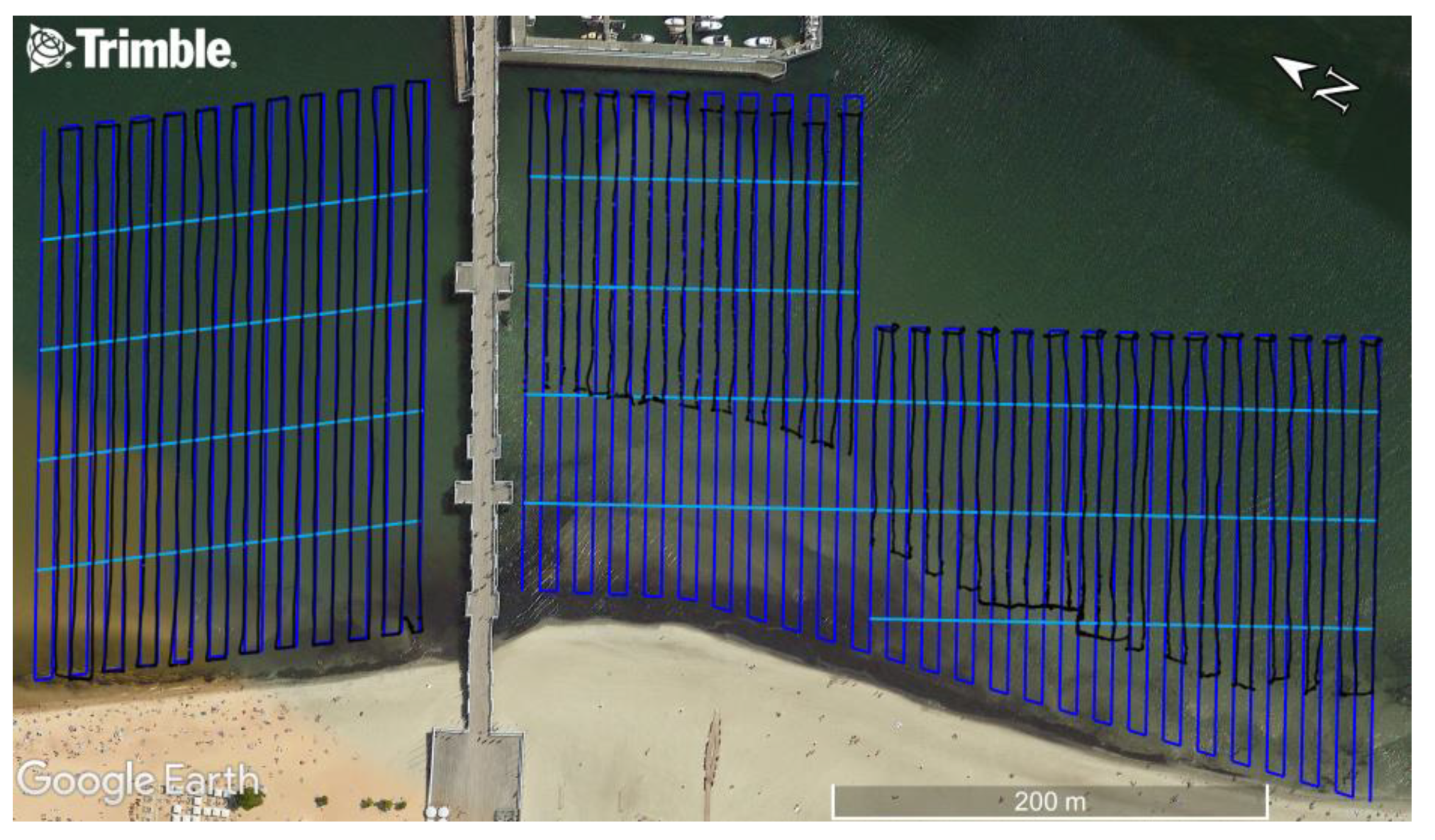
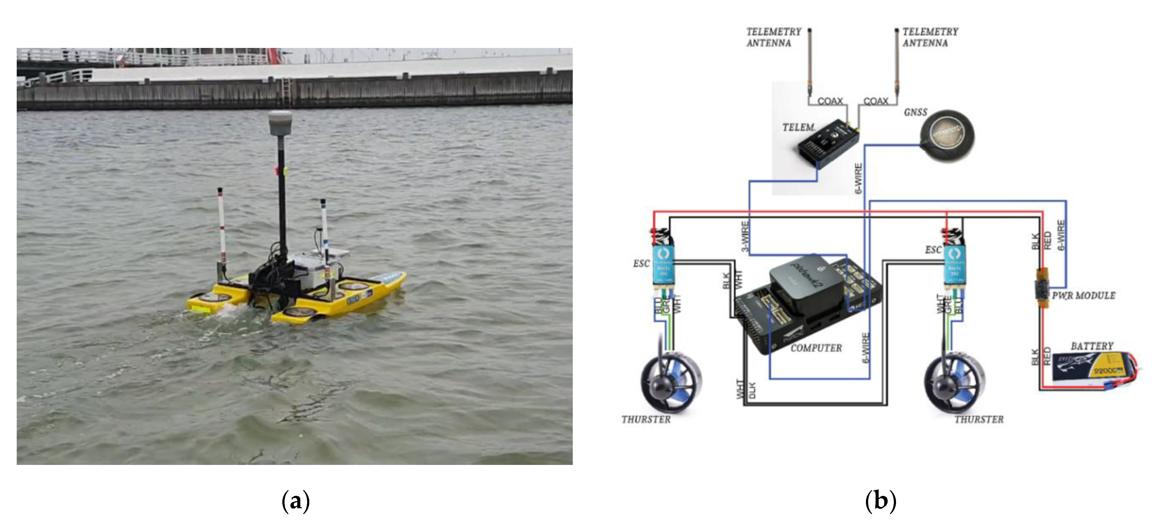
2.1. Hydrographic Surveys Carried Out Using a USV

On 26 November 2019, at 09:00 am–02:56 pm, bathymetric surveys of the waterbody adjacent to the Sopot pier were carried out. The hydrometeorological conditions prevailing in the area under study were the main factor determining the time of the measurements. For this reason, the surveys were undertaken during sea states of 1–2 degrees in the Douglas sea scale, and at a wind force of 3 degrees in the Beaufort scale. To determine the predicted weather conditions (sea current, waves, wind), short-term weather forecasts were provided online by the Institute of Meteorology and Water Management-National Research Institute (IMGW-PIB) [47], and the data from the Baltic Environmental Satellite Remote Sensing System (SatBałtyk) [48] were used. During the study, the sea level was rather stable and ranged from 472 to 476 cm in relation to the Kronstadt height system (PL-KRON86-NH). Relevant data were acquired from a tide gauge station located in Gdynia, 10 km north of the Sopot pier, which is closest to the location of measurement performance [49,50].

The next operation to be performed before carrying out the hydrographic surveys was the planning of sounding profiles along which the USV was designed to move in automatic mode. For the study, the following were designed: 73 main profiles located perpendicular to the coastline, and five control profiles located parallel to the coastline. Moreover, to prevent damage to the measuring equipment and the vehicle itself, the first sounding profile was planned at a distance of no less than 10 m from the coastline determined based on the most up-to-date orthophotomap provided on the Google Earth Pro. It was also assumed that the mutual distance between the sounding lines would be 8 m for main profiles and 50 m for control profiles (Figure 1). The direction, the shape, and the distance between sounding lines were determined based on the following standards: “IHO Standards for Hydrographic Surveys” [51], “NOS Hydrographic Surveys Specifications and Deliverables” [52] and “EM 1110-2-1003 USACE Standards for Hydrographic Surveys” [53], as well as national recommendations, books, and publications on hydrography [54,55,56].

Before the bathymetric surveys were commenced, the measuring equipment needed to be mounted on the USV. It comprised the following devices: a SonarMite BTX Single Beam Echo Sounder (SBES) for depth measurements with an accuracy of 1 cm + 0.5% depth; a Trimble R10 GNSS receiver which, by using a selected GNSS geodetic network, enables the performance of measurements in real-time with an accuracy of 1–2 cm (p = 0.95) in three dimensional coordinates; and a 3DR PX4 Pixhawk autopilot used to control an USV in the automatic mode based on readings from a low-cost GPS/GLONASS receiver (u-blox NEO-M8N) [57]. The geodetic receiver and the echo sounder transducer were placed on a relatively short pole (with a length of approx. 1 m), which is mounted in a special grip firmly fixed to the USV, i.e., on an H-shaped steel mounting frame connecting both hulls. Other devices, such as an echo sounder, a GNSS receiver controller, and an autopilot, were placed in two plastic containers protecting them against the impact of water (Figure 2) [5].

After the mounting of all measuring devices on the USV, the sensors were calibrated to verify their correct operation and to eliminate errors. Therefore, for a SBES, three operations were performed [58]:

(1)

Calibration (taring) of the vertical echo sounder.

(2)

Measurement of the vertical distribution of the speed of sound in water.

(3)

Measurement of the draft of the echo sounder transducer.

However, for the GNSS receiver, the following operations were carried out:

(1)

Inclinometer calibration.

(2)

Magnetometer calibration.

As regards the Proportional-Integral-Derivative (PID) controller, three controllers had to be set. First, the throttling valve (acceleration) controller. Then, the angular velocity (following the order to turn) controller. Finally, the navigational controller. PID controller parameters were set by a manual method [59].

The SBES taring process was carried out on the water when the USV was situated near the coastline at a depth of approx. 0.5 m. Initially, a wooden calibrating board was placed on the waterbody seabed under the echo sounder transducer. The depth between the transducer and the board was then determined. Subsequently, the depth measured using a hydroacoustic device was compared to the depth determined with a measuring tape. When the difference between the measured depths was greater than 1 cm, the depths recorded by the SBES were corrected.

After performing all the above-presented operations, the main part of the research was commenced. During the tests, the USV took measurements of 21,685 points. It is particularly noteworthy that due to the low seakeeping of the vehicle (approximately 20 kg) and the wind prevailing in this region, it proved extremely difficult to maintain the drone along the planned sounding profiles.

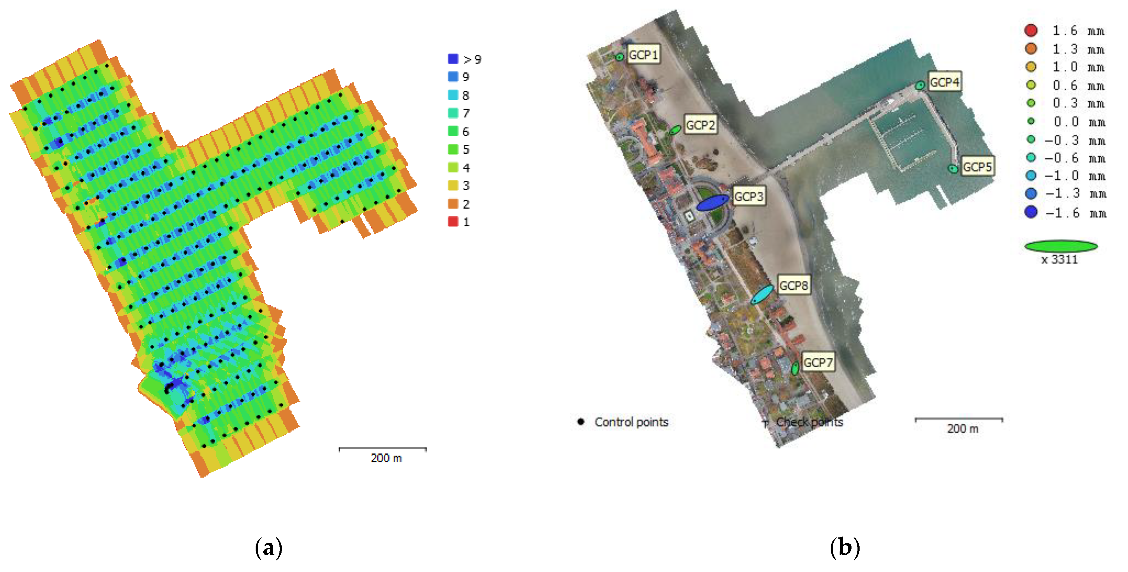
2.2. Photogrammetric Measurements Carried Out Using a UAV

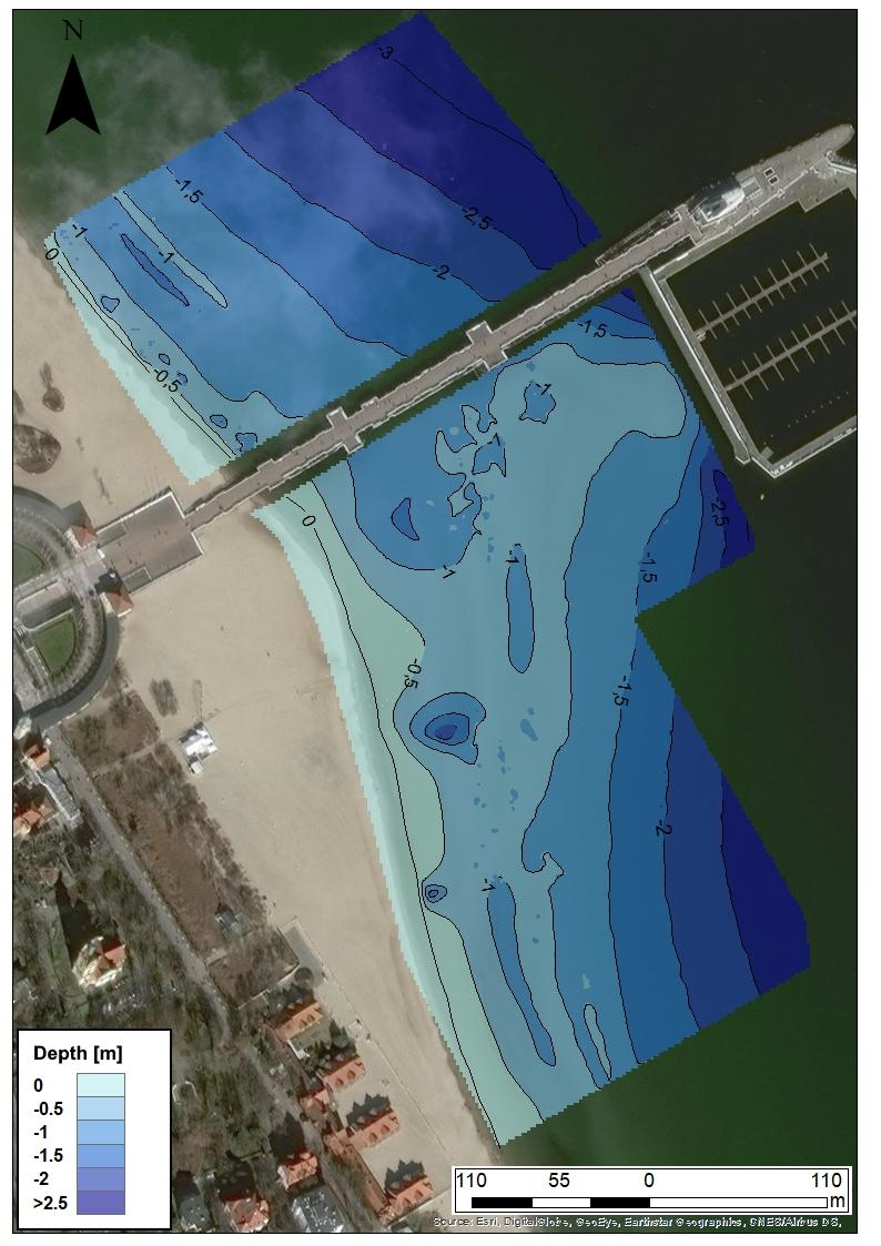
On 23 November 2019, photogrammetric measurements of the area adjacent to the Sopot pier were carried out to investigate the unique phenomenon known as tombolo which occurs in the vicinity [24]. The study was carried out using a DJI Mavic Pro 2 UAV (

Table 1. Selected technical data for the DJI Mavic Pro 2 Unmanned Aerial Vehicle (UAV).

Parameter	Parameter Value
Dimensions (length × width × height) [mm]	322 × 242 × 84
Weight [g]	907
Max ascent speed [m/s]	5
Max descent speed [m/s]	3
Max speed [km/h]	72
Max service ceiling [m]	6000
Max flight time [min]	31
Max hovering time [min]	29
Overall flight time [min]	25
Max flight distance [km]	18
Operating temperature range [°C]	−10 to 40
Satellite positioning systems	GPS/GLONASS

) equipped with a Hasselblad stabilized visible light camera (

Table 2. Selected technical data for the Hasselblad camera and sensor.

Parameter	Parameter Value
Sensor	1-inch CMOS Effective pixels: 20 million
Pixel size [μm]	2.41
Lens	Field Of View (FOV): about 77° 35 mm format equivalent: 28 mm Aperture: f/2.8–f/11 Shooting range: 1 m to ∞
ISO range	100–12800 (photo), 100–6400 (video)
Shutter speed	8–1/8000 s
Still image size [pixels]	5472 × 3648
Still photography modes	Single shot Burst shooting: 3/5 frames Auto Exposure Bracketing (AEB): 3/5 bracketed frames at 0.7 EV Bias Interval (JPEG: 2/3/5/7/10/15/20/30/60 s, RAW: 5/7/10/15/20/30/60 s)
Video resolution	4K: 3840 × 2160 24/25/30 p 2.7K: 2688 x 1512 24/25/30/48/50/60 p FHD: 1920 × 1080 24/25/30/48/50/60/120 p
Photo format	JPEG, DNG (RAW)
Video format	MP4, MOV (MPEG-4 AVC/H.264, HEVC/H.265)

). The UAV used in the study is representative of commercial platforms, designed and intended mainly for recreational flights and for amateur filmmakers. These types of UAVs are often used for photogrammetric tasks, primarily due to their popularity, reliability, ease of use and programming, and good study results [60,61].

The photogrammetric flights were programmed and carried out at an altitude of 100 m in accordance with the single grid plan, with a longitudinal and lateral overlap set at 65% (Figure 3a) as a result of the compromise between required point cloud quality [62,63], computation time [64], available time slot for the flight execution, weather and wind conditions [62], and terrain and modeling surface characteristics [61]. Due to the extent of the area and the wind blowing at more than 5 m/s, the planned flight time exceeded the maximum safe time for the UAV used. Therefore, it was decided to divide the area under study into three smaller testing areas. This enabled the performance of three flights lasting for 18 min each, and the total coverage of the area under study. A total of 462 photographs were taken during the measurements.

Photogrammetric data processing was performed using Agisoft Metashape software. The calculation process starts with importing the total number of photographs. After loading the photographs, the process of image adjustment begins. During a flight, geographic coordinates that are determined while the UAV’s GNSS receiver is taking a photograph are assigned to each recorded image. Such a process, referred to as direct georeferencing [65], significantly accelerates the process of photograph adjustment and the subsequent aerotriangulation. During the adjustment process, the software detects tie points on subsequent overlapping images. To detect tie points, it is required that an appropriate number of structures and textures be present in common areas recorded on several photographs (Figure 3a). Due to the relatively low flight altitude (100 m) and the nature of the area being recorded, it was not possible to detect tie points on the photographs that included only the water surface area with no other fixed structures recorded. Such a situation made it possible to find tie points and to adjust a block of images from 233 photographs. If it was necessary to image the water surface over a larger area adjacent to the indicated structure, the flight altitude would need to be increased so that the photographs would cover a larger area with clear fixed points. Such a procedure is possible; however, it contributes to an increase in the field pixel, which, in the case under analysis, decreases the quality of the photogrammetric study. The selection of the flight altitude is usually determined by the accuracy requirements of the study, and in low-ceiling aerial photogrammetry it is a compromise between quality and physical possibilities for performing a flight over an area under study. The maximum flight altitude is limited by technical parameters and the duration of a UAV flight, regulations, and the air traffic, while the minimum altitude is limited by the highest field structures and the requirements for the safe separation of a flight from these structures. In this case, the maximum permissible flight altitude was up to 100 m and was limited by the Military Aerodrome Traffic Zone (MATZ).

The application of direct georeferencing enables the preparation of a photogrammetric study (orthophotomaps, a Digital Terrain Model (DTM)) in a specific reference system (usually it is the World Geodetic System 1984 (WGS 84) ellipsoid); however, the positioning accuracy for the GNSS receiver mounted on the UAV does not correspond to the accuracies dedicated to surveying applications. To obtain the expected accuracies for photogrammetric studies, it is necessary to perform measurements of the Ground Control Points (GCPs) and use them to properly fit the photogrammetric study. To this end, seven GCPs were used (Figure 3b), whose coordinates were determined using a Trimble R10 GNSS receiver. Control points were evenly distributed over the area under study, which allowed accuracy of 1.56 cm Root Mean Square (RMS) to be achieved.

Results of the processing of photogrammetric measurements include an orthophotomap (Figure 4a) and a DTM (Figure 4b) of the area adjacent to the Sopot pier.

3. Results

After the completion of photogrammetric measurements using an UAV (carried out on 23 November 2019) and hydrographic surveys using an USV (carried out on 26 November 2019), preparations began for processing them to develop a bathymetric chart of the waterbody adjacent to the Sopot pier.

It was first necessary to remove the depths erroneously recorded by the echo sounder. The bathymetric data processing procedure was based on rejecting measurements with gross errors e.g., depths which several times exceeded values in the immediate vicinity of the considered point. The second step was measurement sampling relative to the density criterion. An acceptable distance interval between adjacent points in the horizontal plane was set at 50 cm. The process of removing erroneously recorded depths was carried out by a manual method using Cloud Compare software. Next, the selected depths had to be referred to the so-called chart datum which, for the PL-KRON86-NH height system, amounts to 508 cm [50]. To do so, the following formula should be used:

$$d’=-\left(d+\Delta d_{ET}\pm \Delta d_{CD}\right)$$

(1)

where:

$d’$—normal height of the point measured by echo sounder in the PL-KRON86-NH height system (cm),

$d$—depth measured by the echo sounder (cm),

$\Delta d_{ET}$—draft of the echo sounder transducer (cm),

$\Delta d_{CD}$—a depth correction referred to the chart datum in the PL-KRON86-NH height system (cm), which needs to be added where the averaged sea level (${\overline{d}}_{SL}$) does not exceed 508 cm; otherwise, it needs to be subtracted.

The correction $\Delta d_{CD}$, which is determined based on the following equation, requires additional explaination:

$$\Delta d_{CD}=508 cm-{\overline{d}}_{SL}$$

(2)

where:

${\overline{d}}_{SL}$—averaged sea level observed on a tide gauge between consecutive full hours in the PL-KRON86-NH height system (cm). It can be determined based on the data provided by the IMGW–PIB weather service (Figure 5).

Bathymetric data processed in this way were loaded into the ArcGIS software.

Subsequently, the DTM adjacent to the Sopot pier, generated based on the performed photogrammetric measurements, had to be uploaded to the ArcGIS software to create the coastline. Similarly to the depths measured by the echo sounder, an isobath of 0 m had to be referred to the average sea level in the PL-KRON86-NH height system. To create the coastline of the waterbody, a tool for creating contour lines (which determines them by the interpolation method) was used.

On the other hand, the generated coastline and the selected points measured by the echo sounder had to be reduced to a uniform geodetic reference system. Therefore, during the data processing, inter alia, the Gaussa–Krüger projection, the Universal Transverse Mercator (UTM) system (used for issuing nautical charts), the PL-KRON86-NH height system, and a PL-geoid-2011 quasigeoid model, were used [66]. After unifying the three-dimensional position coordinates, the creation of a DTM model in the ArcGIS software began. To generate it, the natural neighbor interpolation was used, i.e., one of the methods for seabed modeling that is most frequently applied in hydrography [67,68,69]. It should be noted that depths of the area located between the coastline and the 0.3 m isobath (determined by the minimum range of the echo sounder) have been interpolated due to the lack of real measurement data. Additionally, besides the DTM model, isobaths were created at 0.5 m intervals, which were presented in the form of smooth curves using the spline method [46]. Finally, it was decided to add the orthophotomap provided by the ESRI company to the DTM and the isobaths marked on it (Figure 6).

It follows from Figure 6 that the tombolo oceanographic phenomenon concerned is developing to the east of the Sopot pier. On the other hand, in the western part of the waterbody, the phenomenon practically does not occur as the isobaths (0–3 m) are located parallel to the coastline and at equal distances. The most noticeable differences in bathymetry can be seen between the yacht marina and the beach located to the east of the pier. Isobaths in this region do not increase linearly as they move away from the coastline, which results in the alternating “shallows” and “depressions” with depths ranging from 1 to 1.5 m. On the basis of our measurement results it was concluded that for 37% of the area under analysis, the seabed depth is no more than 1 m, while for 64% of the surface area of the waterbody, it does not exceed 1.5 m.

However, most importantly, the depths in the yacht mooring area near the pier and the marina range from 1 to 1.5 m, and pose a serious navigational hazard which may result in damaging the hull structure. The draft of both sailing and motorized vessels often exceeds 1–1.5 m, thus preventing them from sailing on these waters. It should be added that sailors may not be aware of this fact because the official Electronic Navigational Chart (ENC) [70], developed in 2011, suggests that isobaths increase linearly (and at equal distances) in relation to the beach coastline, and the water depth for the berthing area ranges from 2 to 3.5 m (Figure 7). Moreover, based on the chart, it can be concluded that the tombolo phenomenon stops developing at a distance of 300–400 m to the east from the Sopot pier [26].

Research has shown that, with the integration of hydrographic and photogrammetric data obtained using autonomous unmanned measurement platforms, it is possible to carry out terrain relief surveys at the land-water interface zone, meeting the requirements of the International Hydrographic Organization (IHO) Special Order [51]. It was also found that the main difficulty is to determine the depth between the coastline and the minimum depth recorded by the echo sounder (this area is devoid of real measurement data).

4. Discussion

The article presents the methodology for carrying out measurements of the tombolo oceanographic phenomenon using unmanned aerial and surface vehicles, based on the example of the waterbody adjacent to the Sopot pier. In addition to the research methodology, it also presents the measurement results carried out in November 2019 within this area.

The analyses performed indicate that currently the most effective and optimal method from the point of view of accuracy, coverage, and rate is the realization of bathymetric surveys in ultra-shallow waters (at depths of less than 1 m) using an USV on which a multi-GNSS receiver and a miniature SBES or a MultiBeam EchoSounder (MBES) can be mounted [71,72,73,74,75]. The measurements performed in the littoral zone can be supplemented with the use of an UAV equipped with a high-resolution camera [76,77,78,79,80]. However, it should be remembered that measurements using unmanned aerial and surface vehicles can be carried out during favorable weather conditions. Based on previous experience, hydrographic surveys in the coastal zone with the use of a vessel weighing about a dozen kg can be performed in small waves (sea state 0–1 in the Douglas scale) and low wind (wind strength 0–1 in the Beaufort scale). Wind blowing at 10 km/h (2 on the Beaufort scale) forms small wind waves of 10–20 cm on the water surface, which can have an adverse effect on the vessel stability and on the sounding profile (with no significant heel) [50]. The same applies to photogrammetric measurements carried out using UAVs. Air missions must be carried out under appropriate meteorological conditions [81,82]. Flights must not be performed during precipitation events, although it is possible to perform flights under a low cloud ceiling or under foggy or windy conditions, provided that the wind speed does not exceed 6–7 m/s. Therefore, in terms of the quality of the images taken, it is recommended that the photogrammetric flight pass using a drone be carried out on a sunny, windless day at the recommended low flight ceiling.

The use of unmanned aerial and surface vehicles to monitor processes in the coastal zone is a new approach. Based on the analysis of the literature, two publications were found in which unmanned measurement platforms were used in hydrographic and photogrammetric surveys at the land-water interface zone [20,83]. In the article from 2018 [20] they were applied for the detection and mapping of beachrock formations lying on very shallow waters (0–0.7 m), while in the publication from 2019 [83] they were used to determine the terrain relief to calculate the storage capacity loss of water in the river. Research has shown that the use of unmanned measurement platforms in the coastal zone is better in terms of accuracy, coverage, and rate than current solutions applied by hydrographers, such as: the tachymetric method [1,3], the geodetic method employing a GNSS receiver in real time [50,84], and the hydrographic method in which a manned vessel is used to determine the water depth [10,26].

Based on the 3D map (Figure 6), it must be concluded that the tombolo phenomenon occurring near the Sopot pier creates many problems, including a navigational hazard to sailing, particularly in the vicinity of the yacht marina. Due to its shallow waters (1–1.5 m), this region is not suitable for safe maneuvering of either motorized or sailing vessels. Additionally, the bathymetric data measured in 2019 deviate by approx. 2 m from those provided on official ENC from 2011, thus possibly making sailors unaware of this state of affairs [26]. Moreover, as demonstrated by the results of other authors’ studies, the tombolo phenomenon has an adverse effect on both the aquatic environment and humans. It results, inter alia, in the cyanobacteria blooming and other bacteria which prevents bathing and swimming in this region repeatedly during the year [85,86,87]. Additionally, despite the positive fact that the Sopot beach is expanding (under reconstruction), in other places the sand reaching the pier is taken away. This is particularly noticeable on the Orłowo Cliff, which is part of the Kępa Redłowska nature reserve. The gradual sliding of the cliff is a result of the sand accumulation near the marina in Sopot [88].

The main cause of tombolo formation in Sopot are waves coming to the coast diffracted around the marina walls; therefore, the wave energy behind the marina wall is much smaller than the wave energy coming from the deep sea. Reduced amount of energy in the area between the marina wall and the coast causes the sedimentation of debris transported by waves. The mechanism of tombolo formation between the marina wall and the coast is due to the system of double eddies (directed towards each other) and wave diffraction on both walls, perpendicular to the shore [89].

In the next stages of the research, the authors intend to determine seasonal changes in the tombolo phenomenon in Sopot, as well as during extreme weather phenomena such as storms. In addition, in order to determine the depth of the shallow waterbody (between the coastline and the minimum depth recorded by the echo sounder), it is planned to perform the analysis of high-resolution images taken by an UAV. They will be determined based on the pixel image radiometry.

References

1. Lane, S.N.; Richards, K.S.; Chandler, J.H. Developments in monitoring and modelling small-scale river bed topography. Earth Surf. Process. Landf. 1994, 19, 349–368. [Google Scholar] [CrossRef]
2. Westaway, R.M.; Lane, S.N.; Hicks, D.M. Remote Sens. of clear-water, shallow, gravel-bed rivers using digital photogrammetry. Photogramm. Eng. Remote Sens. 2001, 67, 1271–1282. [Google Scholar]
3. Koljonen, S.; Huusko, A.; Mäki-Petäys, A.; Louhi, P.; Muotka, T. Assessing habitat suitability for juvenile Atlantic salmon in relation to in-stream restoration and discharge variability. Restor. Ecol. 2012, 21, 344–352. [Google Scholar] [CrossRef]
4. Baptista, P.; Bastos, L.; Bernardes, C.; Cunha, T.; Dias, J. Monitoring sandy shores morphologies by DGPS—A practical tool to generate digital elevation models. J. Coast. Res. 2008, 24, 1516–1528. [Google Scholar] [CrossRef]
5. Specht, C.; Specht, M.; Cywiński, P.; Skóra, M.; Marchel, Ł.; Szychowski, P. A new method for determining the territorial sea baseline using an unmanned, hydrographic surface vessel. J. Coast. Res. 2019, 35, 925–936. [Google Scholar] [CrossRef]
6. Hogrefe, K.R.; Wright, D.J.; Hochberg, E.J. Derivation and integration of shallow-water bathymetry: Implications for coastal terrain modeling and subsequent analyses. Mar. Geod. 2008, 31, 299–317. [Google Scholar] [CrossRef]
7. Kulawiak, M.; Chybicki, A. Application of Web-GIS and geovisual analytics to monitoring of seabed evolution in South Baltic Sea coastal areas. Mar. Geod. 2018, 41, 405–426. [Google Scholar] [CrossRef]
8. Warnasuriya, T.W.S.; Gunaalan, K.; Gunasekara, S.S. Google Earth: A new resource for shoreline change estimation—Case study from Jaffna Peninsula, Sri Lanka. Mar. Geod. 2018, 41, 1–35. [Google Scholar] [CrossRef]
9. Song, F.; Gong, S.; Zhou, R. Underwater topography survey and precision analysis based on depth sounder and CORS-RTK technology. IOP Conf. Ser. Mater. Sci. Eng. 2020, 780, 1–8. [Google Scholar] [CrossRef]
10. Specht, C.; Weintrit, A.; Specht, M. Determination of the territorial sea baseline—Aspect of using unmanned hydrographic vessels. TransNav Int. J. Mar. Navig. Saf. Sea Transp. 2016, 10, 649–654. [Google Scholar] [CrossRef] [Green Version]
11. Stateczny, A.; Błaszczak-Bąk, W.; Sobieraj-Żłobińska, A.; Motyl, W.; Wisniewska, M. Methodology for processing of 3D multibeam sonar big data for comparative navigation. Remote Sens. 2019, 11, 2245. [Google Scholar] [CrossRef] [Green Version]
12. Zwolak, K.; Wigley, R.; Bohan, A.; Zarayskaya, Y.; Bazhenova, E.; Dorshow, W.; Sumiyoshi, M.; Sattiabaruth, S.; Roperez, J.; Proctor, A.; et al. The autonomous underwater vehicle integrated with the unmanned surface vessel mapping the Southern Ionian Sea. The winning technology solution of the Shell Ocean Discovery XPRIZE. Remote Sens. 2020, 12, 1344. [Google Scholar] [CrossRef] [Green Version]
13. Romano, A.; Duranti, P. Autonomous unmanned surface vessels for hydrographic measurement and environmental monitoring. In Proceedings of the FIG Working Week 2012, Rome, Italy, 6–10 May 2012. [Google Scholar]
14. Stateczny, A.; Kazimierski, W.; Burdziakowski, P.; Motyl, W.; Wisniewska, M. Shore construction detection by automotive radar for the needs of autonomous surface vehicle navigation. ISPRS Int. J. Geo Inf. 2019, 8, 80. [Google Scholar] [CrossRef] [Green Version]
15. Giordano, F.; Mattei, G.; Parente, C.; Peluso, F.; Santamaria, R. MicroVEGA (Micro Vessel for Geodetics Application): A marine drone for the acquisition of bathymetric data for GIS applications. Int. Arch. Photogramm. Remote Sens. Spat. Inf. Sci. 2015, XL-5-W5, 123–130. [Google Scholar] [CrossRef] [Green Version]
16. Giordano, F.; Mattei, G.; Parente, C.; Peluso, F.; Santamaria, R. Integrating sensors into a marine drone for bathymetric 3D surveys in shallow waters. Sensors 2016, 16, 41. [Google Scholar] [CrossRef] [Green Version]
17. Genchi, S.A.; Vitale, A.J.; Perillo, G.M.E.; Seitz, C.; Delrieux, C.A. Mapping topobathymetry in a shallow tidal environment using low-cost technology. Remote Sens. 2020, 12, 1394. [Google Scholar] [CrossRef]
18. Mancini, F.; Dubbini, M.; Gattelli, M.; Stecchi, F.; Fabbri, S.; Gabbianelli, G. Using Unmanned Aerial Vehicles (UAV) for high-resolution reconstruction of topography: The structure from motion approach on coastal environments. Remote Sens. 2013, 5, 6880–6898. [Google Scholar] [CrossRef] [Green Version]
19. Zanutta, A.; Lambertini, A.; Vittuari, L. UAV photogrammetry and ground surveys as a mapping tool for quickly monitoring shoreline and beach changes. J. Mar. Sci. Eng. 2020, 8, 52. [Google Scholar] [CrossRef] [Green Version]
20. Nikolakopoulos, K.G.; Lampropoulou, P.; Fakiris, E.; Sardelianos, D.; Papatheodorou, G. Synergistic use of UAV and USV data and petrographic analyses for the investigation of beachrock formations: A case study from Syros Island, Aegean Sea, Greece. Minerals 2018, 8, 534. [Google Scholar] [CrossRef] [Green Version]
21. Turner, I.L.; Harley, M.D.; Drummond, C.D. UAVs for coastal surveying. Coast. Eng. 2016, 114, 19–24. [Google Scholar] [CrossRef]
22. Bandini, F.; Olesen, D.; Jakobsen, J.; Kittel, C.M.M.; Wang, S.; Garcia, M.; Bauer-Gottwein, P. Technical note: Bathymetry observations of inland water bodies using a tethered single-beam sonar controlled by an unmanned aerial vehicle. Hydrol. Earth Syst. Sci. 2018, 22, 4165–4181. [Google Scholar] [CrossRef] [Green Version]
23. Specht, C.; Świtalski, E.; Specht, M. Application of an autonomous/unmanned survey vessel (ASV/USV) in bathymetric measurements. Pol. Marit. Res. 2017, 24, 36–44. [Google Scholar] [CrossRef] [Green Version]
24. Masnicki, R.; Specht, C.; Mindykowski, J.; Dąbrowski, P.; Specht, M. Accuracy analysis of measuring X-Y-Z coordinates with regard to the investigation of the tombolo effect. Sensors 2020, 20, 1167. [Google Scholar] [CrossRef] [PubMed] [Green Version]
25. Specht, C.; Mindykowski, J.; Dąbrowski, P.; Maśnicki, R.; Marchel, Ł.; Specht, M. Metrological aspects of the tombolo effect investigation—Polish case study. In Proceedings of the 2019 IMEKO TC-19 International Workshop on Metrology for the Sea (IMEKO 2019), Genova, Italy, 3–5 October 2019. [Google Scholar]
26. Specht, M.; Specht, C.; Mindykowski, J.; Dąbrowski, P.; Maśnicki, R.; Makar, A. Geospatial modeling of the tombolo phenomenon in Sopot using integrated geodetic and hydrographic measurement methods. Remote Sens. 2020, 12, 737. [Google Scholar] [CrossRef] [Green Version]
27. Owens, E.H. Tombolo. In Beaches and Coastal Geology, Encyclopedia of Earth Science, 1984 ed.; Springer: Boston, MA, USA, 1982. [Google Scholar]
28. De Mahiques, M.M. Tombolo. In Encyclopedia of Estuaries. Encyclopedia of Earth Sciences Series, 2016 ed.; Kennish, M.J., Ed.; Springer: Dordrecht, The Netherlands, 2016; pp. 713–714. [Google Scholar]
29. Benac, Č.; Bočić, N.; Ružić, I. On the origin of both a recent and submerged tombolo on Prvić Island in the Kvarner area (Adriatic Sea, Croatia). Geol. Croat. 2019, 72, 195–203. [Google Scholar] [CrossRef]
30. Otto, J.; Smith, M. Geomorphological mapping. In Geomorphological Techniques; Clarke, L.E., Nield, J.M., Eds.; British Society for Geomorphology: London, UK, 2013; pp. 1–10. [Google Scholar]
31. Booij, N.; Holthuijsen, L.H.; Ris, R.C. The “SWAN” wave model for shallow water. In Proceedings of the 25th International Conference on Coast. Eng. (ICCE 1996), Orlando, FL, USA, 2–6 September 1996. [Google Scholar]
32. Hansom, J.D. St Ninian’s tombolo, Shetland. In Coastal Geomorphology of Great Britain; May, V.J., Hansom, J.D., Eds.; Joint Nature Conservation Committee: Peterborough, UK, 2003; pp. 458–462. [Google Scholar]
33. Vu, M.T.; Lacroix, Y.; Nguyen, V.T. Empirical equilibrium beach profiles along the eastern tombolo of Giens. J. Mar. Sci. Appl. 2018, 17, 241–253. [Google Scholar] [CrossRef]
34. Schwartz, M.L.; Grano, O.; Pyokari, M. Spits and tombolos in the southwest archipelago of Finland. J. Coast. Res. 1989, 5, 443–451. [Google Scholar]
35. Kim, H. Three-dimensional sediment transport model. PhD Thesis, University of Liverpool, Liverpool, UK, 1993. [Google Scholar]
36. O’Connor, B.A.; Nicholson, J. A three-dimensional model of suspended particulate sediment transport. Coast. Eng. 1998, 12, 157–174. [Google Scholar] [CrossRef]
37. Kuroiwa, M.; Kamphuis, J.W.; Kuchiishi, T.; Matsubara, Y.; Noda, H. Medium-term Q-3D coastal area model with shoreline change around coastal structures. In Proceedings of the 29th International Conference on Coast. Eng. (ICCE 2004), Lisbon, Portugal, 19–24 September 2004. [Google Scholar]
38. Watanabe, A.; Maruyama, K.; Shimizu, T.; Sakakiyama, T. Numerical prediction model of three-dimensional beach deformation around a structure. Coast. Eng. Jpn. 1986, 29, 179–194. [Google Scholar] [CrossRef]
39. Shimizu, T.; Kumagai, T.; Watanabe, A. Improved 3-D beach evolution model coupled with the shoreline model (3D-SHORE). In Proceedings of the 25th International Conference on Coast. Eng. (ICCE 1996), Orlando, FL, USA, 2–6 September 1996. [Google Scholar]
40. Jörissen, J.G.L. Strandhoofden Gemodelleerd in Delft3D-RAM: Strandhoofden Als Instrument Voor Het Regelen van Het Langstransport. Master’s Thesis, Delft University of Technology, Delft, The Netherlands, 2001. [Google Scholar]
41. Nam, P.T. Numerical Model of Beach Topography Evolution due to Waves and Currents. Special Emphasis on Coastal Structures. Available online: https://pdfs.semanticscholar.org/c5af/bff0cb81a3dff8f2cc3528016c85bb1b1107.pdf?_ga=2.233758174.1954626850.1580128302-234920152.1580128302 (accessed on 19 March 2020).
42. Kuchiishi, T.; Kato, K.; Kuroiwa, M.; Matsubara, Y.; Noda, H. Applicability of 3D morphodynamic model with shoreline change using a quasi-3D nearshore current model. In Proceedings of the 14th International Offshore and Polar Engineering Conference (ISOPE 2004), Toulon, France, 23–28 May 2004. [Google Scholar]
43. Roelvink, D.; Giles, L.; van der Wegen, M. Morphological modelling of the wet-dry interface at various timescales. In Proceedings of the 7th International Conference on Hydroscience and Engineering (ICHE 2006), Philadelphia, PA, USA, 10–13 September 2006. [Google Scholar]
44. van Koningsveld, M.; van Kessel, T.; Walstra, D.-J.R. A hybrid modelling approach to coastal morphology. In Proceedings of the 5th Coastal Dynamics International Conference (CD 2005), Barcelona, Spain, 4–8 April 2005. [Google Scholar]
45. Kim, H.; Lee, S.; Park, D.; Lim, H.S. Simulation of tombolo evolution by using CST3D-WA. Vibroengineering PROCEDIA 2017, 12, 196–201. [Google Scholar]
46. Specht, M.; Specht, C.; Wąż, M.; Dąbrowski, P.; Skóra, M.; Marchel, Ł. Determining the variability of the territorial sea baseline on the example of waterbody adjacent to the municipal beach in Gdynia. Appl. Sci. 2019, 9, 3867. [Google Scholar] [CrossRef] [Green Version]
47. IMGW-PIB. Fishermans Forecast. Available online: http://baltyk.pogodynka.pl/index.php?page=2&subpage=6&data=25 (accessed on 19 March 2020). (In Polish).
48. Ostrowska, M.; Darecki, M.; Krężel, A.; Ficek, D.; Furmańczyk, K. Practical applicability and preliminary results of the Baltic environmental satellite Remote Sens. system (Satbałtyk). Pol. Marit. Res. 2015, 22, 43–49. [Google Scholar] [CrossRef] [Green Version]
49. IMGW-PIB. Pogodynka.pl—IMGW-PIB Weather Service. Available online: http://pogodynka.pl/ (accessed on 19 March 2020). (In Polish).
50. Specht, M.; Specht, C.; Wąż, M.; Naus, K.; Grządziel, A.; Iwen, D. Methodology for performing territorial sea baseline measurements in selected waterbodies of Poland. Appl. Sci. 2019, 9, 3053. [Google Scholar] [CrossRef] [Green Version]
51. International Hydrographic Organization. IHO Standards for Hydrographic Surveys, 5th ed.; Special Publication No. 44; IHO: Monte Carlo, Monaco, 2008. [Google Scholar]
52. National Oceanic and Atmospheric Administration. NOS Hydrographic Surveys Specifications and Deliverables; NOAA: Silver Spring, MD, USA, 2017. [Google Scholar]
53. United States Army Corps of Engineers. EM 1110-2-1003 USACE Standards for Hydrographic Surveys; USACE: Washington, DC, USA, 2013.
54. Kierzkowski, W. Marine Measurements. Part. I. Hydrographic Measurements; Polish Naval Academy Publishing House: Gdynia, Poland, 1984; Volume 1. (In Polish) [Google Scholar]
55. Sciortino, J.A. Fishing Harbour Planning, Construction and Management; Food and Agriculture Organization of the United Nations: Rome, Italy, 2010. [Google Scholar]
56. Stenborg, E. The Swedish parallel sounding method state of the art. Int. Hydrogr. Rev. 1987, 64, 7–14. [Google Scholar]
57. Specht, M.; Specht, C.; Lasota, H.; Cywiński, P. Assessment of the steering precision of a hydrographic Unmanned Surface Vessel (USV) along sounding profiles using a low-cost multi-Global Navigation Satellite System (GNSS) receiver supported autopilot. Sensors 2019, 19, 3939. [Google Scholar] [CrossRef] [Green Version]
58. Grządziel, A. Single beam echo sounder in hydrographic surveys. Marit. Rev. 2006, 4, 11–28. (In Polish) [Google Scholar]
59. Wikipedia, the Free Encyclopedia. PID Controller. Available online: https://en.wikipedia.org/wiki/PID_controller#Manual_tuning (accessed on 19 March 2020). (In Polish).
60. Burdziakowski, P. Low cost real time UAV stereo photogrammetry modelling technique—Accuracy considerations. E3S Web Conf. 2018, 63, 1–5. [Google Scholar] [CrossRef]
61. Burdziakowski, P. UAV in todays photogrammetry—Application areas and challenges. In Proceedings of the 18th International Multidisciplinary Scientific GeoConference (SGEM 2018), Albena, Bulgaria, 2–8 July 2018. [Google Scholar]
62. Dandois, J.P.; Olano, M.; Ellis, E.C. Optimal altitude, overlap, and weather conditions for computer vision UAV estimates of forest structure. Remote Sens. 2015, 7, 13895–13920. [Google Scholar] [CrossRef] [Green Version]
63. Yoo, Y.H.; Choi, J.W.; Choi, S.K.; Jung, S.H. Quality evaluation of orthoimage and DSM based on fixed-wing UAV corresponding to overlap and GCPs. J. Korean Soc. Geospat. Inf. Syst. 2016, 24, 3–9. [Google Scholar]
64. Torres-Sánchez, J.; López-Granados, F.; Borra-Serrano, I.; Manuel Peña, J. Assessing UAV-collected image overlap influence on computation time and digital surface model accuracy in olive orchards. Precis. Agric. 2018, 19, 115–133. [Google Scholar] [CrossRef]
65. Burdziakowski, P. Towards precise visual navigation and direct georeferencing for MAV using ORB-SLAM2. In Proceedings of the 2017 Baltic Geodetic Congress (BGC Geomatics 2017), Gdańsk, Poland, 22–25 June 2017. [Google Scholar]
66. Council of Ministers of the Republic of Poland. Ordinance of the Council of Ministers of 15 October 2012 on the National Spatial Reference System; Council of Ministers of the Republic of Poland: Warsaw, Poland, 2012. (In Polish)
67. Kogut, T.; Niemeyer, J.; Bujakiewicz, A. Neural networks for the generation of sea bed models using airborne lidar bathymetry data. Geod. Cartogr. 2016, 65, 41–53. [Google Scholar] [CrossRef] [Green Version]
68. Sassais, R.; Makar, A. Methods to generate numerical models of terrain for spatial ENC presentation. Annu. Navig. 2011, 18, 69–81. [Google Scholar]
69. Wu, C.Y.; Mossa, J.; Mao, L.; Almulla, M. Comparison of different spatial interpolation methods for historical hydrographic data of the lowermost Mississippi River. Ann. GIS 2019, 25, 133–151. [Google Scholar] [CrossRef]
70. Stateczny, A.; Gronska-Sledz, D.; Motyl, W. Precise bathymetry as a step towards producing bathymetric electronic navigational charts for comparative (terrain reference) navigation. J. Navig. 2019, 72, 1623–1632. [Google Scholar] [CrossRef]
71. Kurowski, M.; Thal, J.; Damerius, R.; Korte, H.; Jeinsch, T. Automated survey in very shallow water using an unmanned surface vehicle. IFAC PapersOnLine 2019, 52, 146–151. [Google Scholar] [CrossRef]
72. Li, C.; Jiang, J.; Duan, F.; Liu, W.; Wang, X.; Bu, L.; Sun, Z.; Yang, G. Modeling and experimental testing of an unmanned surface vehicle with rudderless double thrusters. Sensors 2019, 19, 2051. [Google Scholar] [CrossRef] [Green Version]
73. Mu, D.; Wang, G.; Fan, Y.; Qiu, B.; Sun, X. Adaptive trajectory tracking control for underactuated unmanned surface vehicle subject to unknown dynamics and time-varing disturbances. Appl. Sci. 2018, 8, 547. [Google Scholar] [CrossRef] [Green Version]
74. Stateczny, A.; Burdziakowski, P.; Najdecka, K.; Domagalska-Stateczna, B. Accuracy of trajectory tracking based on nonlinear guidance logic for hydrographic unmanned surface vessels. Sensors 2020, 20, 832. [Google Scholar] [CrossRef] [Green Version]
75. Yang, Y.; Li, Q.; Zhang, J.; Xie, Y. Iterative learning-based path and speed profile optimization for an unmanned surface vehicle. Sensors 2020, 20, 439. [Google Scholar] [CrossRef] [PubMed] [Green Version]
76. Angnuureng, D.B.; Jayson-Quashigah, P.-N.; Almar, R.; Stieglitz, T.C.; Anthony, E.J.; Aheto, D.W.; Addo, K.A. Application of shore-based video and unmanned aerial vehicles (drones): Complementary tools for beach studies. Remote Sens. 2020, 12, 394. [Google Scholar] [CrossRef] [Green Version]
77. Burdziakowski, P.; Tysiąc, P. Combined close range photogrammetry and terrestrial laser scanning for ship hull modelling. Geosciences 2019, 9, 242. [Google Scholar] [CrossRef] [Green Version]
78. Casella, E.; Drechsel, J.; Winter, C.; Benninghoff, M.; Rovere, A. Accuracy of sand beach topography surveying by drones and photogrammetry. Geo Mar. Lett. 2020, 40, 255–268. [Google Scholar] [CrossRef] [Green Version]
79. Laporte-Fauret, Q.; Marieu, V.; Castelle, B.; Michalet, R.; Bujan, S.; Rosebery, D. Low-cost UAV for high-resolution and large-scale coastal dune change monitoring using photogrammetry. J. Mar. Sci. Eng. 2019, 7, 63. [Google Scholar] [CrossRef] [Green Version]
80. Lowe, M.K.; Adnan, F.A.F.; Hamylton, S.M.; Carvalho, R.C.; Woodroffe, C.D. Assessing reef-island shoreline change using UAV-derived orthomosaics and digital surface models. Drones 2019, 3, 44. [Google Scholar] [CrossRef] [Green Version]
81. Kacprzak, M.; Wodziński, K. Execution of photo mission by manned aircraft and unmanned aerial vehicle. Trans. Inst. Aviat. 2016, 2, 130–141. (In Polish) [Google Scholar] [CrossRef]
82. Witek, M.; Jeziorska, J.; Niedzielski, T. Possibilities of using unmanned air photogrammetry to identify anthropogenic transformations in river channel. Landf. Anal. 2013, 24, 115–126. (In Polish) [Google Scholar] [CrossRef]
83. Erena, M.; Atenza, J.F.; García-Galiano, S.; Domínguez, J.A.; Bernabé, J.M. Use of drones for the topo-bathymetric monitoring of the reservoirs of the Segura River Basin. Water 2019, 11, 445. [Google Scholar] [CrossRef] [Green Version]
84. Specht, C.; Weintrit, A.; Specht, M.; Dąbrowski, P. Determination of the territorial sea baseline—Measurement aspect. IOP Conf. Ser. Earth Environ. Sci. 2017, 95, 1–10. [Google Scholar] [CrossRef] [Green Version]
85. Sopot City Hall. 2016: Tombolo Connects the Beach with the Marina. Available online: https://sopot.gmina.pl/raport-marina-tombolo-2016/ (accessed on 19 March 2020). (In Polish).
86. Sopot NaszeMiasto.pl. Sopot Beach to be Corrected again. Alignment is in Progress. Available online: http://sopot.naszemiasto.pl/artykul/sopocka-plaza-znowu-do-poprawki-trwa-wyrownywanie-zdjecia,2253932,artgal,t,id,tm.html (accessed on 19 March 2020). (In Polish).
87. Sopot NaszeMiasto.pl. Sopot is Growing! The Concrete Marina forms a Sand Peninsula at the Pier. Available online: http://sopot.naszemiasto.pl/artykul/sopot-sie-powieksza-betonowa-marina-tworzy-przy-molu,1772082,artgal,t,id,tm.html (accessed on 19 March 2020). (In Polish).
88. Trójmiasto.Wyborcza.pl. A Sand Island has Grown up at the Pier in Sopot. The Sand on the Cliff in Gdynia is Decreasing. Available online: http://trojmiasto.wyborcza.pl/trojmiasto/1,35612,20860078,wyrosla-piaskowa-wyspa-przy-molo-w-sopocie-ubywa-za-to-piasku.html (accessed on 19 March 2020). (In Polish).
89. Institute of Oceanology of the Polish Academy of Sciences. Conducting Research and Modeling of the Seafloor and Sea Shore near the Pier in Sopot. Available online: https://bip.umsopot.nv.pl/Download/get/id,32756.html (accessed on 9 June 2019).
Figure 1. The planned main profiles (blue color) and control profiles (light blue color) along with the plotted trajectory of the Unmanned Surface Vehicle (USV) (black color) during hydrographic surveys of the waterbody adjacent to the Sopot pier.
Jmse 08 00384 g001
Figure 2. Unmanned Surface Vehicle (USV) with measuring equipment mounted to it (a) and a schematic diagram of the main components of the USV after the modernization of the control system from remote to automatic mode (b) [57].
Jmse 08 00384 g002
Figure 3. The location of the camera and the overlap (the number of images that present a particular surface is marked with appropriate colors) (a) and the distribution of control points with the position error indicated (the horizontal position error by the ellipse shape and the vertical position error is presented by the ellipse color) (b).
Jmse 08 00384 g003
Figure 4. An orthophotomap (a) and a Digital Terrain Model (DTM) (b) of the area adjacent to the Sopot pier.
Jmse 08 00384 g004
Figure 5. A diagram of sea level variability observed on a tide gauge in Gdynia according to the Institute of Meteorology and Water Management—National Research Institute (IMGW—PIB) weather service.
Jmse 08 00384 g005
Figure 6. A bathymetric chart of the waterbody adjacent to the Sopot pier, developed based on hydrographic and photogrammetric measurements carried out in November 2019.
Jmse 08 00384 g006
Figure 7. A bathymetric chart of the waterbody adjacent to the Sopot pier, based on an official Electronic Navigational Chart (ENC) from 2011.
Jmse 08 00384 g007