Heat Vulnerability and Heat Island Mitigation in the United States

Abstract

Heat waves are the deadliest type of natural hazard among all weather extremes in the United States. Given the observed and anticipated increase in heat risks associated with ongoing climate change, this study examines community vulnerability to extreme heat and the degree to which heat island mitigation (HIM) actions by state/local governments reduce heat-induced fatalities. The analysis uses all heat events that occurred over the 1996–2011 period for all United States counties to model heat vulnerability. Results show that: (1) Higher income reduces extreme heat vulnerability, while poverty intensifies it; (2) living in mobile homes or rental homes heightens susceptibility to extreme heat; (3) increased heat vulnerability due to the growth of the elderly population is predicted to result in a two-fold increase in heat-related fatalities by 2030; and (4) community heat island mitigation measures reduce heat intensities and thus heat-related fatalities. Findings also show that an additional locally implemented measure reduces the annual death rate by 15%. A falsification test rules out the possibility of spurious inference on the life-saving role of heat island mitigation measures. Overall, these findings inform efforts to protect the most vulnerable population subgroups and guide future policies to counteract the growing risk of deadly heat waves.

1. Introduction

Heat waves are the deadliest type of natural hazard among all weather extremes in the United States (USA). Every year, more than 1000 heat events occur, causing an average of 131 direct heat fatalities during the last twenty years. However, excess heat exposure contributes to a far greater number of deaths, directly and indirectly—658 deaths per year on average during the years 1999–2009 according to National Center for Health Statistics (NCHS) [1]. The risk of extreme heat has been elevated in many regions of the world including the USA as extreme weather phenomena is increasing in both frequency and magnitude under global climate change [2,3]. The observed and predicted shifts in the variability and intensity of weather extremes that are driven by climate change, such as heat waves, flooding, droughts, and tornadoes have been discussed in many scientific studies [4,5,6,7]. With regard to heat events, [4] and [6] predict that future heat waves in North America will occur more frequently with greater intensity and longer duration. [8] estimates that extreme temperatures due to climate change will result in a loss of 1.3 million life-years annually in the USA by the end of 21st century.

Increasing frequency of weather extremes in recent decades coupled with predictions about climate change triggered policy efforts and community actions for hazard mitigation and adaptation [9,10]. The most relevant heat-related actions currently undertaken by state and local governments in the USA are the community-based “heat island” reduction activities [11]. The statewide or community level actions database contains all 172 actions and are publicly available from the United States Environmental Protection Agency (EPA) website https://www.epa.gov/heat-islands/heat-island-community-actions-database. Heat island reduction measures include trees and vegetation, green roofs, cool roofs, and cool pavements; these strategies are implemented through demonstration projects (e.g., green roof installation), incentive programs (e.g., tax abatements or rebates), urban forestry and community tree planting programs (e.g., Million Trees Initiative in Los Angeles, New York City, Denver, etc.), and outreach and education programs. The primary goal of community heat island reduction measures is to reduce a populated area’s elevated surface/atmospheric temperatures. Heat island reduction actions are important heat hazard mitigation measures in that they help to limit temperature rise in risk areas.

Previous studies on heat waves from a disaster vulnerability perspective have been mostly conducted by epidemiologists, sociologists, or geographers. These studies are primarily interested in the temperature–mortality relationship; most of them use daily all-cause mortality of the study area to find factors that can explain the increase in mortality during (and in the aftermath of) heat waves. Some studies examine vulnerability using excess mortality due to high temperature of certain areas in the USA [12,13,14], or in an international context [15,16,17]. Other researchers examine the impact of a large heat event as a case study [18,19]. Another large set of studies focuses on the construction and/or evaluation of a heat vulnerability index for a certain region in the USA [20,21,22,23].

The present study takes a different analytical approach. We examine every individual heat event and the resulting direct deaths that occurred across the USA within every county over 14 years. Our findings differ from previous studies in several respects. First, the modelling of heat wave impacts on society is structurally different—previous heat studies use all-cause mortality while this study uses direct heat-induced fatalities. As a result of using all-cause mortality, it is not obvious in those studies whether the factors found to be significantly contributing to mortality indicate true “heat” vulnerability factors, or just those associated with general mortality. Second, epidemiological studies apply case-oriented approaches, thus their findings are often not comparable to each other and not easily generalizable across different spatial or temporal contexts. The present article constructs a model of USA nationwide heat fatalities at a local scale, utilizing both spatial and temporal variations while controlling for regional fixed effects. Finally, none of the previous studies empirically address political and institutional aspects, whereas we seek to identify the role of community-based heat island mitigation actions initiated by state/local governments in reducing heat intensities and resulting fatalities. However, in both strands of the heat study literature, the importance of social vulnerability components in defining overall place vulnerability to heat are emphasized. We build upon the findings of previous heat studies to construct an integrative conceptual framework of heat vulnerability.

We draw on prior disaster vulnerability research from multiple disciplines to construct a framework that integrates the climatic, built-environmental, and socio-economic elements of disaster vulnerability. A fundamental notion of this integrative framework is that heat vulnerability is defined and shaped not only by physical and meteorological characteristics of the hazard itself, but also the various human components such as built-environmental conditions, population characteristics, and socio-economic factors. Within this framework, we empirically analyze the dynamics of heat vulnerability, taking into consideration meteorological socio-economic factors as well as heat hazard mitigation efforts.

Our empirical analysis involves the modeling of two critical components of heat vulnerability. For the first component, the heat hazard mitigation model, we use county-year panel structured data for years 1998–2011 to evaluate the role of heat island reduction measures in mitigating heat hazard intensity. We employ the random trend model that controls for both county-fixed effects and county-specific time trends. In the second component, we consider a heat vulnerability–fatality model, where we examine all county-level heat and excessive heat events over the 1996–2011 period to analyze a wide range of meteorological and anthropogenic determinants of heat-induced fatalities. Considering the nature of the non-panel structured heat event data with excess zero fatalities, we employ the zero-inflated negative binomial (ZINB). Lastly, we directly estimate the effects of heat island mitigation (HIM) measures on heat fatalities using the Poisson fixed effects estimator, controlling for the unobserved county heterogeneity.

Our two-part analysis shows that because of the long-lasting and synergistic effects of the heat island mitigation (HIM) measures, the heat intensity reductions of such measures accumulate. Thus, counties with more mitigation actions are progressively less vulnerable to extreme heat than counties with fewer activities. We also find that an additional locally implemented measure reduces annual death rates (deaths per heat event) by 14.87%. Urbanization as measured by the urban population density tends to increase the adverse impacts of heat waves, leading to more fatalities. The analysis also confirms that higher income reduces vulnerability to heat waves, while poverty intensifies it. Housing related factors are critical predictors of heat wave fatalities; living in mobile homes or rental homes increases disaster vulnerability. Also, population composition is important; heat vulnerability is greater in counties with higher proportions of elderly, young, and non-white populations. Findings suggest that the socially isolated elderly and the elderly living in poverty are the most heat-vulnerable population sub-groups. Notably, heightened heat vulnerability due to the growth of the elderly population is predicted to result in a two-fold increase in heat fatalities by 2030.

The rest of this article is organized as follows. In the next two sections, we discuss the risks of extreme heat in the USA and community heat island mitigation actions. In Section 3, we provide a summary of extreme heat events across the USA, and in Section 4 we present the modeling, data, and empirical methods we use in the analysis. In Section 5, we offer a discussion of our results, and Section 6 concludes the article.

2. Risk of Extreme Heat in the USA

Heat waves are not as destructive as other types of natural hazards such as hurricanes or tornadoes; however, extreme heat is by far the deadliest type of hazard among all weather extremes in the USA. Heat waves place considerable stress on the human body, causing heat exhaustion or heat stroke, which could lead to death. Every year, more than 1000 heat events occur, causing hundreds of deaths and even more heat-related illnesses. Over the past twenty years, heat resulted in an average of 131 direct deaths each year (NWS). However, extreme heat also exacerbates underlying health problems. A National vital statistics report from National Center for Health Statistics (NCHS) [1] showed that during 11 years from 1999 to 2009, extreme heat exposure resulted in 7233 deaths, where heat was the underlying cause for about 70% of the fatalities and a contributing factor for remaining 30%. Notwithstanding heat-induced illnesses and injuries, annual heat-related mortality of 658 is about five-times larger than the reported number of deaths certified as heat illness. These figures show the profound adverse impacts of extreme heat on people’s health and lives.

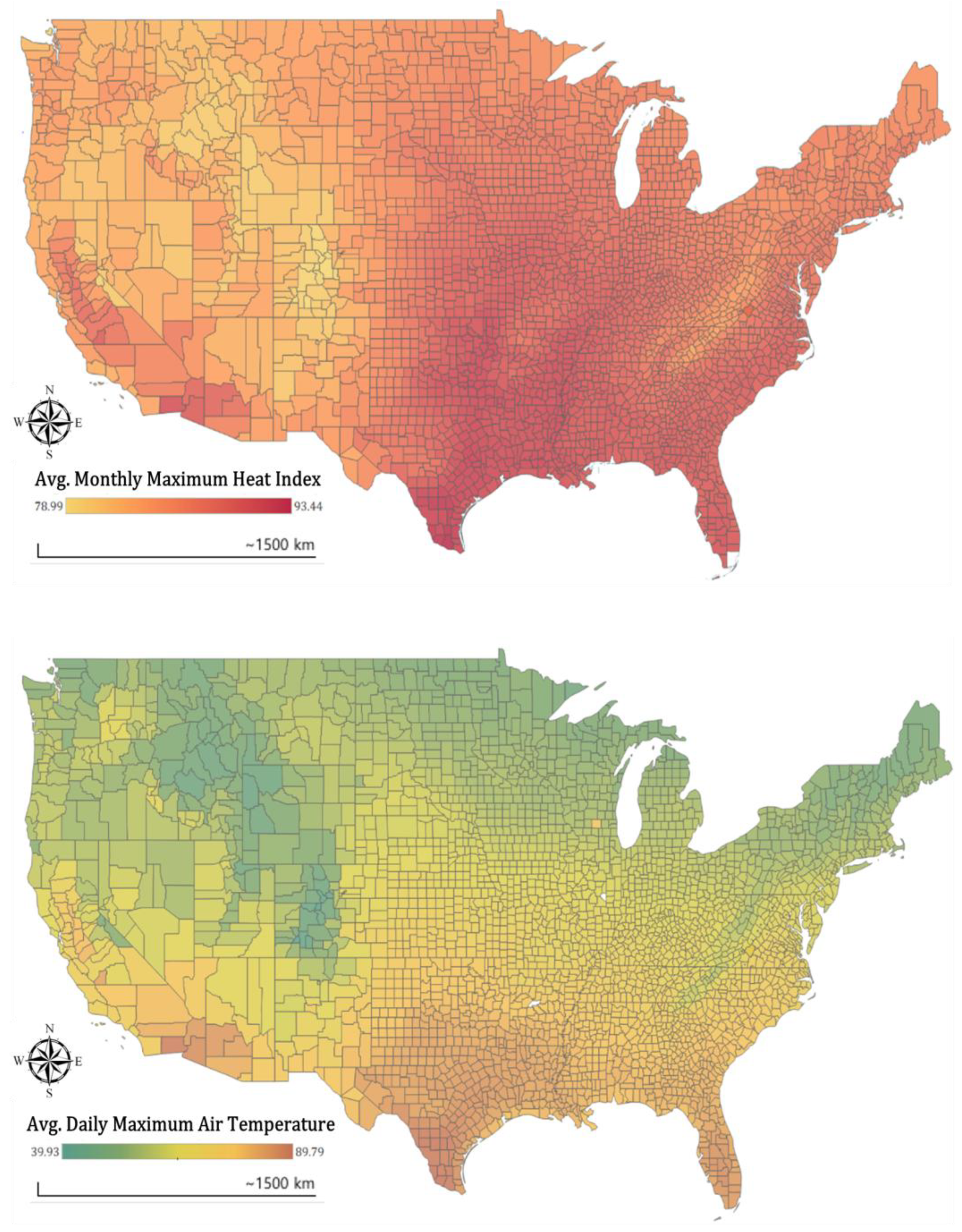
Before discussing heat waves and their impacts on people, it is important to correctly understand the definition and related measures of heat events. Like the Fujita-scale for tornadoes, there is a heat index measure for heat waves. The United States National Oceanic and Atmospheric Administration National Weather Service (NOAA NWS) defines the heat index as “a subjective measure of what it feels like to the human body when relative humidity is factored into the actual air temperature”. This implies that heat events result from a combination of high temperatures and high humidity. Figure 1 compares the summertime average maximum heat index (i.e., apparent temperature) and the average daily maximum temperature. The figure clearly shows that temperature alone does not fully explain the risk of heat across the USA regions. Compared to dry hot areas in the Western region of the USA that includes states such as Nevada, Utah, and New Mexico, humid regions in the Midwest and Eastern USA have relatively higher heat index values. Excessive heat or heat events occur as reported in the NOAA Storm Events Database whenever heat index values meet or exceed locally/regionally established excessive heat warning or heat advisory thresholds, respectively. The definition/determination of heat and excessive heat are provided in

Table A1. Determination of heat and excess heat.

Determination of a Heat Category Event in NWS Storm Data
Heat
A period of heat results from the combination of high temperatures (above normal) and relative humidity. A heat event occurs and is reported in Storm Data whenever heat index values meet or exceed locally/regionally established heat advisory thresholds. Fatalities or major impacts on human health occurring when ambient weather conditions meet heat advisory criteria are reported using the heat event. If the ambient weather conditions are below heat advisory criteria, a heat event entry is permissible only if a directly related fatality occurred due to unseasonably warm weather, and not man-made environments.
Excess Heat
Excessive heat results from a combination of high temperatures (well above normal) and high humidity. An Excessive heat event occurs and is reported in Storm Data whenever heat index values meet or exceed locally/regionally established excessive heat warning thresholds. Fatalities (directly related) or major impacts to human health that occur during excessive heat warning conditions are reported using this event category. If the event that occurred is considered significant, even though it affected a small area, it should be entered into Storm Data.

Source: National Weather Service Instruction 10-1605 (MARCH 23, 2016) Operations and Services Performance, Storm Data Preparation. (http://www.nws.noaa.gov/directives/).

in the Appendix A. The Storm Events Database managed by NOAA’s National Centers for Environmental Information (NCEI) is available at https://www.ncdc.noaa.gov/stormevents/ftp.jsp.

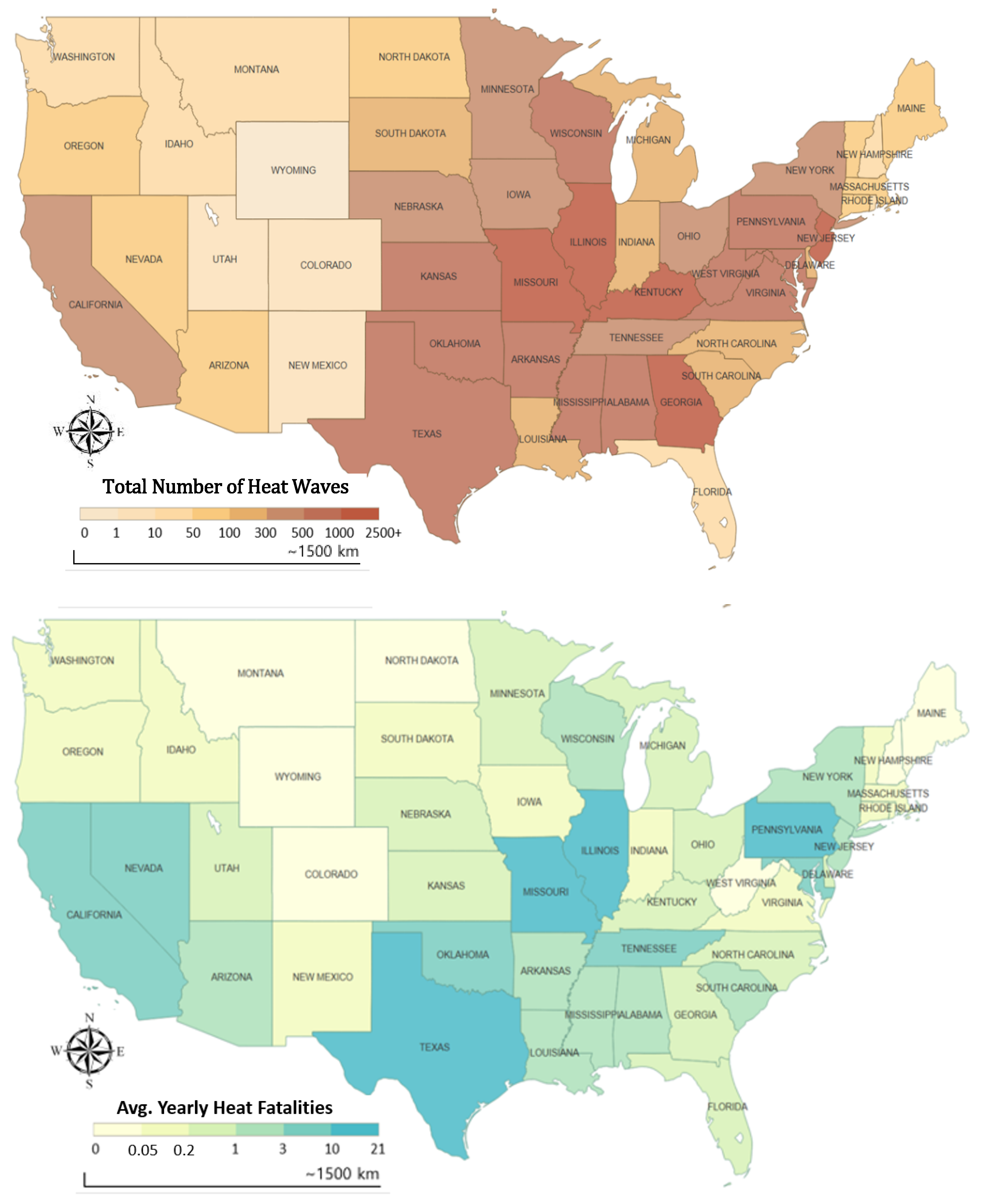
Figure 2 shows the average fatality of extreme heat events by state in the contiguous USA over the 20 years from 1996 to 2015, respectively. In general, most heat waves occur in the southern part of the country including western regions, and the Great Plains. Areas west of the Rocky Mountains exhibit high temperature; however, as both temperature and humidity are both factored, dry hot areas in western states such as Wyoming, Utah, and Colorado rarely have heat events. Missouri, Illinois, New Jersey, Georgia, and Kentucky are the top five states that experience the most extreme heat events, whereas the top five states with the highest death tolls are Illinois, Pennsylvania, Texas, Missouri, and Nevada. The human impacts of extreme heat are not proportionally distributed across the regions. The differences as reflected in Figure 1 and Figure 2 hint at the importance of societal and human components in determining disaster vulnerability.

Moreover, there are mounting concerns about the risk of heat waves in the USA; climate scientists predict that heat events will become more devastating with an increase in both magnitude and frequency of extreme heat phenomena [2,3]. The work of [4] indicates that future heat waves in North America will become “more intense, more frequent, and longer lasting.” Also, the fifth assessment report of the UN Intergovernmental Panel on Climate Change (IPCC) [6] summarizes predictions from climate models as follows: “it is ‘virtually certain’ that there will be more frequent hot and fewer cold temperature extremes over most land areas as global mean temperatures increase and it is ‘very likely’ that heat waves will occur with a higher frequency and duration.” The observed and anticipated increase in the risk of heat waves and their silent yet catastrophic impacts has drawn considerable attention from scholars in various disciplines, policy makers, and the media. In the following sections, we discuss state and local government efforts to mitigate the growing risk of heat hazards and briefly review the multi-disciplinary literature on disaster vulnerability.

3. Community Heat Island Mitigation (HIM) Actions

Increasing outbreaks of weather extremes in recent decades and associated gloomy predictions about climate change has triggered policy efforts and community actions for hazard mitigation and adaptation. The most relevant heat-related actions currently undertaken by state and local government in the USA are community-based “heat island” reduction activities. As of May 2018, a total of 172 statewide or community level actions are publicly available at the U.S. Environmental Protection Agency (EPA) website https://www.epa.gov/heat-islands/heat-island-community-actions-database. The primary goal of the community heat island mitigation measures is to lower the developed area’s elevated surface/atmospheric temperatures, thereby reducing the risk of heat waves. Under the heat island phenomena, annual mean air temperature of a city with one million or more people can be 1.8 to 5.4 °F (1 to 3 °C) warmer than air in surrounding areas [11]. The main causes of urban heat islands are reduced vegetation (i.e., more dry and impervious surfaces), materials used to build urban infrastructure (which reflect/shed less and absorb/store more of the sun’s energy), urban geometry (which affect wind flow, energy absorption, radiation), and anthropogenic heat emission (all the energy used for human activities). Increased temperature due to heat islands has considerable impacts on human life such as detrimental health impacts, added risk of heat waves, impaired water quality, and other adverse environmental impacts [11].

Growing interest and concern among communities regarding heat islands have motivated the development and implementation of heat island reduction strategies by state and local governments in recent decades. Heat island mitigation actions (currently active or completed) are listed by the United States Environmental Protection Agency (EPA). Communities use four main measures to reduce the urban heat island problem: (i) Trees and vegetation; (ii) green roofs, (iii); cool roofs; and (iv) cool pavements. Such strategies are implemented through voluntary or policy mechanisms. Voluntary mechanisms include demonstration projects (e.g., green roof installation), incentive programs (e.g., tax abatement or rebate), urban forestry and community tree planting programs (e.g., Million Trees Initiative in LA, NYC, Denver, etc.), and outreach and education programs. Policy mechanisms involve procurement, ordinances, and standards such as building/zoning code, tree and landscape ordinances, green building programs and standards, as well as comprehensive community plans and design guidelines for heat island reduction.

Table 1. Heat island mitigation actions list by initiation year (1985–2014).

Years	Trees and Vegetation	Cool Roofs	Green Roofs	Cool Pavements	Others (HVI, Master Plan)
	Within-County Actions					Total
1985–1989	2	0	0	0	0	2
1990–1994	2	1	0	0	0	3
1995–1999	4	2	3	1	1	11
2000–2004	19	9	10	8	0	46
2005–2009	35	19	18	23	1	96
2010–2014	22	19	15	15	0	71
Total	84	50	46	47	2	229
	Statewide Actions					Total
1995–1999	0	1	0	0	0	1
2000–2004	2	2	1	0	0	5
2005–2009	3	3	1	0	1	8
2010–2014	6	2	2	3	0	13
Total	11	8	4	3	1	27

Source: Authors’ own calculation using “Heat Island Community Actions Database” (EPA).

presents the total number of community and statewide heat island mitigation measures by type of strategy and by year from 1985 to 2014. During this period, 229 within-county and 27 statewide strategies have been initiated. Except for recently completed demonstration projects (e.g., green roof installation), most efforts have been ongoing since the project was initiated. The number of heat island mitigation adoptions substantially increased since the early 2000s as communities became more aware of the heat island problem and the harmful effects of elevated temperatures. The trees and vegetation measure has been the most popular strategy, followed by cool roofs. About half of the strategies have been implemented through policy mechanisms such as building/zoning codes, ordinances, programs, and standards. The other half have been carried out voluntarily through incentive programs, demonstration projects, and outreach/education.

Heat island mitigation measures address the root causes of growing heat vulnerability by modifying and reducing the long-term likelihood and prevalence of heat risk in populated areas. Heat island mitigation strategies also help communities manage the fundamental meteorological risk of high temperature, thus acting primarily as “heat-hazard mitigation.” For instance, it may not be possible to prevent tornadoes or hurricanes from happening and so efforts are devoted to minimizing the harmful consequences through anticipation, preparedness, disaster warning, and post-disaster relief, etc.,). However, heat events can be potentially averted and thus their negative impacts can be avoided if actions are taken to “cool down” at-risk communities. Given this context, we hypothesize and test the notion that communities that implement heat island mitigation strategies exhibit lower heat intensities as measured by the heat index (i.e., apparent temperature) and in turn, become less vulnerable relative to communities that do not. More details on the heat hazard mitigation model are presented in the next section.

4. Conceptual Framework, Data, and Methodology

Studies of devastating natural disasters have revealed that disaster impacts vary significantly across different population groups with different socio-economic and political status. Numerous social scientists discuss the role of socio-economic characteristics such as poverty, inequalities with regard to gender, age, or ethnicity in determining disaster vulnerability [25,26,27,28,29,30]. Over the past decade, a body of empirical disaster impact research has emerged that demonstrate the multi-faceted nature of disaster vulnerability and use the socio-political ecology of disasters model as a basis for their empirical analyses [14,31,32,33,34,35]. Generally, this strand of literature highlights the socio-economic conditions that exacerbate or alleviate disaster impacts, while some studies pay special attention to political and institutional factors that play a role in determining disaster vulnerability [31,34]. In an international context, a set of studies focus on the relationship between economic development and disaster impacts, demonstrating that economic and institutional factors are important determinants of disaster casualties [36,37,38,39,40].

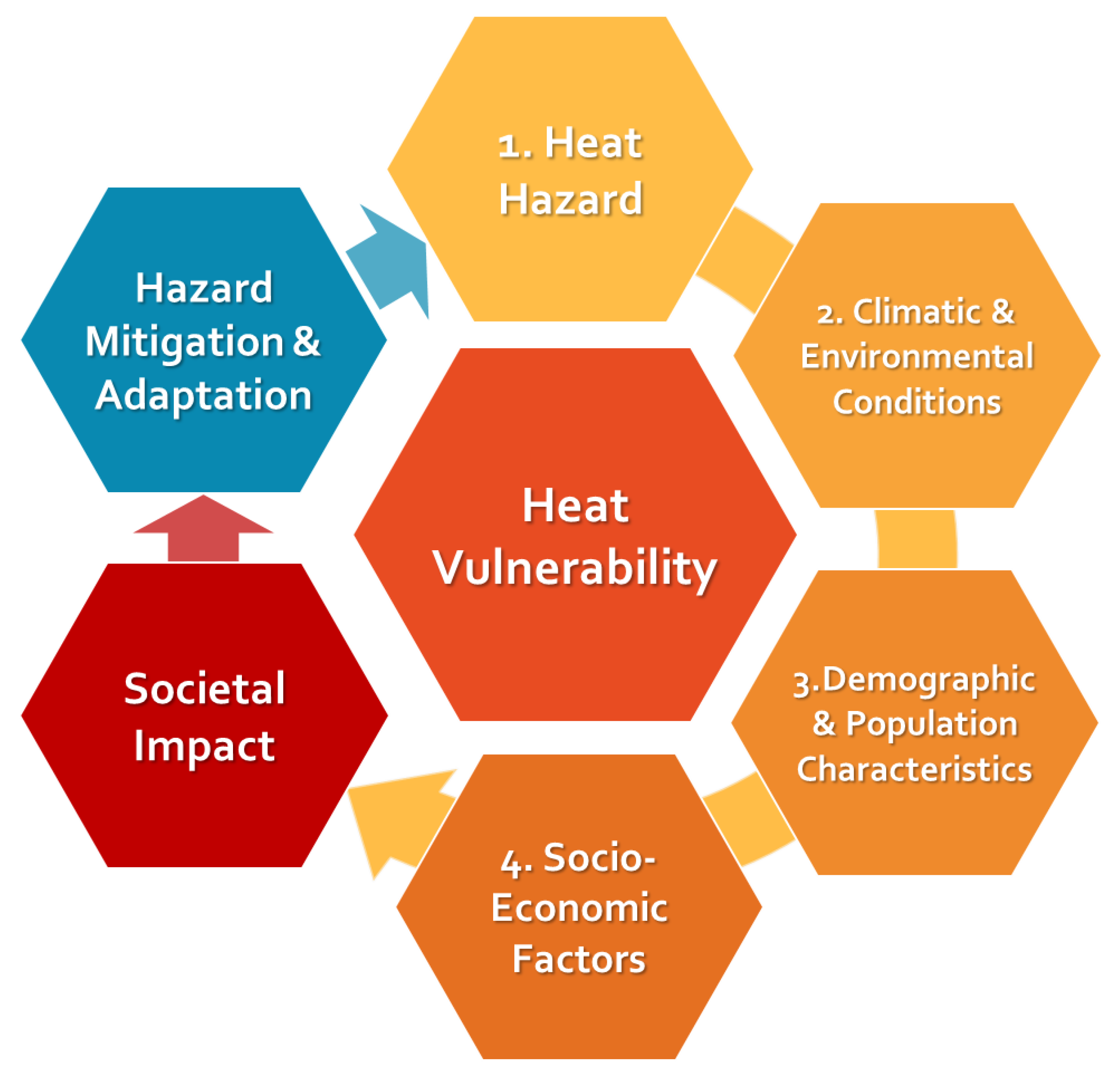
Consolidating the prior findings and knowledge on disaster vulnerability from multiple disciplines, this study applies an integrative view of the climatic, built-environmental, socio-economic, and institutional elements of disaster vulnerability for a comprehensive perspective of heat vulnerability and a robust identification of heat risk factors. To facilitate the understanding of the important linkages and interactions among various the factors, a conceptual framework of our heat vulnerability model is illustrated in Figure 3. As shown in the figure, community disaster vulnerability is multi-faceted; it is defined and shaped not only by physical and meteorological hazard characteristics, but also by various human components such as built-environmental conditions, population characteristics, and socio-economic factors.

Each of the three arrows in the figure indicates important interactions and relationships among the components, which this study is primarily interested in and addresses empirically. The first arrow connects the four key elements that shape “heat vulnerability” and points to “societal impact,” showing that societal outcomes of extreme heat hazards are determined and influenced by the key elements of heat vulnerability. Our main analysis investigates this relationship to identify the underlying societal and environmental factors that determine heat-induced fatalities and then uses the estimation results to predict future outcomes. The second arrow that connects “societal impact” and “hazard mitigation and adaptation,” indicating the shorter-run societal and political pressures for public action for heat mitigation as a reaction to the negative consequences of heat hazards. In the longer-term, public efforts on structural hazard mitigation and adaptation, such as the abovementioned heat island reduction strategies, will modify and ameliorate heat vulnerability by fundamentally reducing the heat hazard risks. This linkage is indicated by the blue arrow pointing to “heat hazard”—the first element of heat vulnerability. Each of the major heat vulnerability components and how they are incorporated in the empirical analysis is discussed in detail in the following subsections.

4.1. Major Components of Heat Vulnerability

Based on the conceptual framework presented in Figure 3, we propose that the major components that determine vulnerability to heat hazards include the: (i) Heat hazard profile; (ii) climatic and environmental conditions; and (iii) demographic and socio-economic characteristics. In addition, we consider institutional mitigation and adaptation efforts as an external factor that influences and interacts with heat vulnerability.

4.1.1. Heat Hazard Profile

The heat hazard profile includes event-specific physical and meteorological aspects of a heat event. We consider factors such as the timing of the incidence (time of day, season of the year when an event occurred), type of the heat event (excessive heat or heat), and heat index value in the month an event occurred. Previous studies on tornadoes and floods [34,41] control for the time of day by categorizing it into overnight (12:00–5:59 a.m.), morning (6:00–11:59 a.m.), early afternoon (12:00–3:59 p.m.), late afternoon (4:00–7:59 p.m.), and evening (8:00–11:59 p.m.), showing that disaster impacts differ depending on the timing of an incident. We also include indicator variables for the seasons (spring, summer, fall, and winter) as control variables. The most critical meteorological factor in our model is the heat index (also known as apparent temperature) that measures the intensity of a heat hazard. Heat intensity is approximated by the average daily maximum heat index value in the month the event occurred. Previous epidemiologic heat studies find a positive correlation between the temperature and all-cause mortality [42]. Although our study examines the direct fatalities resulting from a heat event (instead of all-cause mortality) as an outcome measure, it is expected that a similar or even stronger positive relationship holds between the heat index (apparent temperature) and heat-induced fatalities.

4.1.2. Climatic and Environmental Conditions

Heat vulnerability is also shaped by characteristics of the place exposed to the extreme heat hazard. We take into consideration the area-specific risk factors such as climatic and meteorological conditions of the area (annual average temperature, annual average of max. air temperature) and built-environmental conditions (urbanization/population density). If a heat event occurs in a community that is not accustomed to extreme high temperature and heat hazards, the impact of the heat stressor can potentially be deadlier. In this regard, the annual average air temperature and the average maximum air temperature are included in our model. As discussed earlier, heat island effects can magnify heat vulnerability in urban areas because of the urban structures and land use patterns with less vegetated surfaces relative to rural areas. Considering that urbanization is an important heat risk factor that can exacerbate heat wave impacts, we include urban population density in our model as a measure of urbanization. As an alternative measure of the urbanization, the percent of urban population was also considered. However, because of the strong correlation between the percent of urban population and population size (correlation coefficient = 0.84), we incorporate urban density by controlling for population size in the empirical analysis.

4.1.3. Demographic and Socio-Economic Characteristics

The impacts of extreme weather events on different population segments can vary depending on their social and economic characteristics. Those who are more vulnerable in a social context are also more susceptible to harm in the event of extreme heat. Based on previous studies of heat or other types of natural disasters, we stress that population composition, poverty, income, as well as housing play a role in determining heat vulnerability.

In our heat vulnerability model, demographic composition such as the proportion of the population who are young and elderly and the proportion of the population that is non-white are considered. Many epidemiological studies have shown the differences in heat mortality risk by age where the elderly and children tend to suffer greater health impacts from heat stress because of their limited ability to thermoregulate [43,44]. Race/ethnicity is another key factor that must be taken into account when modeling disaster vulnerability. Prior studies demonstrate that disaster impacts vary by race and ethnicity due to factors such as language barriers, housing patterns, community isolation, and social and economic disparities [45,46]. Our analysis sheds light on which demographic groups are most vulnerable, which in turn can be used to target resources and provide assistance.

We also incorporate several socio-economic factors that determine vulnerability. We consider economic status as measured by county per capita income and the poverty rate. A core interest for research in the economics of natural disasters literature is how the level of economic development or wealth affects disaster impacts [36,37,38,39,40]. In general, these studies find a negative relationship between income and disaster-induced fatalities; wealthier countries have a higher demand for safety where economic resources they possess enable them to employ precautionary measures to mitigate disaster risk. Other studies examine the vulnerability of people who are economically insecure or live below the poverty line [33,47]. [45,48] found that greater poverty increases vulnerability to tornadoes. Heat-episode case studies also find that the majority of the victims of the Midwest heat disaster in 1980 and the Chicago heat waves in 1995 were from low-income groups [18,48].

A last set of human components factored into our heat vulnerability model is housing-related factors—the share of renter occupied housing units and the share of mobile homes among all housing units. Previous studies show that living in low-cost, affordable housing tends to increase disaster vulnerability due to the substandard housing quality [49,50,51]. Both housing factors we consider are closely linked with structural and socio-economic vulnerability to natural hazards. [52] explains that housing ownership and mobile homes are among the most important predictors of social vulnerability. Recent disaster studies [14,33,34,41] provide empirical evidence showing that places with more mobile homes or renter occupied homes suffer greater disaster-induced fatalities. Our empirical evaluation of vulnerability in relation to housing can be used for target assistance during heat events.

4.1.4. Institutional Efforts for Mitigation and Adaptation

We also consider government-initiated mitigation and adaptation efforts as external factors that influence and interact with heat vulnerability. Many scientific simulation or experimental studies have been carried out to assess the microclimate cooling benefits of the heat island measures such as cool roofs [53,54], trees and vegetation [55,56], and cool pavements [54,57]. However, there has been no prior heat study that evaluates the extent to which government-initiated heat island mitigation (HIM) measures reduce heat vulnerability. To fill this significant gap in the literature, we construct a two-phase model in which the first-phase estimates whether communities that implement heat island mitigation measures exhibit lower heat index values (as a measure of heat intensities) than communities that do not. Using the heat index measure as an intermediary variable, we combine the result from the first-phase heat index estimates with the second-phase heat fatality analysis. We also conduct a direct estimation of the life-saving benefit of the heat island mitigation measures on heat-induced fatalities. Our analyses enable us to evaluate the role of heat island mitigation efforts in reducing extreme heat risk and to identify a mediated effect of heat island mitigation measures on heat-induced fatalities. Our empirical analysis involves modeling two phases of heat vulnerability dynamics. Each model is discussed in detail in the following subsections.

4.2. First-Phase: Heat Hazard Mitigation

Heat hazards can be exacerbated by human activities, but they can be also weakened and ameliorated by human efforts. The first-phase model evaluates the role of heat island reduction measures in mitigating heat hazards using data collected at the scale of USA counties. Factors that are known to increase heat hazards include anthropogenic heat emissions, urbanization, climatic conditions, and geographic locations [11]. Considering these contributing factors, we conceptualize the first-phase heat hazard regression model in the following equation:

$$\mathit{H}\mathit{e}\mathit{a}\mathit{t} \mathit{H}\mathit{a}\mathit{z}\mathit{a}\mathit{r}{\mathit{d}}_{\mathit{i}\mathit{t}}={\mathrm{f}(\mathrm{Anthropogenic} \mathrm{Heat}}_{it},{ \mathrm{Urbanization}}_{it},{\mathrm{Climatic} \mathrm{conditions}}_{it},\mathbf{M}\mathbf{i}\mathbf{t}\mathbf{i}\mathbf{g}\mathbf{a}\mathbf{t}\mathbf{i}\mathbf{o}{\mathbf{n}}_{it-2}|c_i, g_{i}t,{\lambda }_t)$$

(1)

where $c_i=$ unobserved county fixed effects, $g_i=$ county specific linear trend, ${\lambda }_t=$ time effects.

For the dependent variable of the first-phase estimation, the heat index (also known as apparent temperature) is used as a measure of the intensity of heat hazards. Specifically, we use the maximum for monthly average of daily maximum. Attention is given to the heat index because it measures the most severe summertime heat events that pose the greatest threat to people. We hypothesize that community efforts for heat hazard mitigation through various “cooling” strategies reduce the impacts of the deadly heatwaves. We also explore alternative specifications using different heat hazard measures. The number of heat wave days are computed at the county level; the totals show the number of heat wave days per county per year. When the geographic area affected by the heatwave spans more than one county, an extreme heat event is counted for each county where measurable observations that met the heat event definition occurred [58]. The number of heat wave days based on (i) the daily maximum heat index and (ii) the net daily heat stress (NDHS) are also used as alternative measures of heat hazard intensity.

Considering the long-lasting effects of heat mitigation strategies (planting trees and vegetation, use of cool materials for roofs and pavements), we construct a county-year heat island mitigation (HIM) actions variable that indicates a cumulative number of the heat island reduction strategies that have been implemented in a county for every year. We then group counties by the number of mitigation measures that have been implemented. Importantly, as the realization of the heat-hazard-lowering effects of the HIM measures may not be immediate, we use 2-year lagged values of the HIM actions variables. To explicitly control for the most important underlying factor that influences the community HIM adoption decisions, we include previous extreme heat risk measured by the sum of heat wave days during the 3-year period prior to any HIM adoption (i.e., heat wave days in t − 3, t − 4, and t − 5). In the regressions, three types of heat island mitigation actions variables are incorporated in each of the three specifications: (a) An indicator variable that represents whether one or more heat island mitigation action has been adopted (=1) or not, (b) a continuous variable for the total number of actions, c) multiple group indicator variables that are constructed based on the number of mitigation actions taken (0, 1, 2–3, 4+). The number of measures of 0, 1, 2–3, 4+ are specifically used to group counties in order to have a sufficient number of observations within each of the group indicators in the regression. In the earlier years of the analysis, there were very limited number of counties that adopted any HIM measures. For example, prior to 2006, counties with two HIM measures make up less than 1% of the total observations.

We use county-year panel structured data to estimate the heat-hazard-reducing effect of heat island mitigation measures using the random trend model while controlling for time effects. The random trend model (RTM) explicitly allows for two sources of heterogeneity—the level effect, $c_i$, and the county-specific linear trend, $g_i$ [59]. In the fixed effects estimation, the unobserved effect is set to have the same partial effect on the heat hazard in all time periods. However, the length of the time dimension of our panel data (1998–2011) is relatively long, during which each county could presumably have its own specific time trend. Allowing for this possibility, we estimate the random trend model, we first difference the Equation (2) to eliminate the level effect, $c_i$, and then apply the fixed effects model to the first-differenced Equation (3) to remove a trend effect, $g_i$.

By employing the random trend model, we control for the geographic location and many other area-specific physical factors that may be related to heat hazards, such as proximity to large water bodies and mountainous terrain but rarely change over time (i.e., time-invariant county traits and characteristics, $c_i$) as well as county-specific trends that could affect the intensity of heat hazards ($g_i)$. A well-known contributing factor of the urban heat island effect, urban growth, is expected to be captured by the county trend effects. A continuing urbanization trend is found nationwide, but the rate of the urban growth may vary across the counties. However, the county level urban population data are only available decennially. The interpolation method is commonly used with decennial data to obtain a monotonic interpolation of the data, i.e., a linear trend. We include the urbanization measure in the fixed effects specification but not in the RTM specification, as the trend effect $g_i$ in the RTM captures county-specific urbanization trends that influence heat hazard intensities. In addition, naturally occurring meteorological temporal variations over time that are common to all counties are absorbed by the vector of time effects, ${\mathit{\lambda }}_{\mathit{t}}$. Thus, any global or macro-scale trend of heat intensity, such as global warming, would be captured by the year effects while a meso-scale heat trend would be controlled for by the county-specific time trends.

$$\mathit{H}{\mathit{I}}_{\mathit{i}\mathit{t} }=c_i+g_{i}t+{\mathit{\beta }}_{\mathbf{1}}{\mathit{M}}_{\mathit{i}\mathit{t}-\mathbf{2}}+\beta ·X_{it}+{\mathit{\lambda }}_{\mathit{t}}+u_{it}\hspace{1em}\hspace{1em}t=3,\dots ,T$$

(2)

$$\Delta \mathit{H}{\mathit{I}}_{\mathit{i}\mathit{t}}=g_i+{\mathit{\beta }}_{\mathbf{1}}\Delta {\mathit{M}}_{\mathit{i}\mathit{t}-\mathbf{2}}+\beta ·\Delta X_{it}+\Delta {\mathit{\lambda }}_{\mathit{t}}+\Delta u_{it},\hspace{1em}t=4,\dots ,T$$

(3)

Annual air temperatures and monthly heat index data for years 1998–2011 are collected from North America Land Data Assimilation System (NLDAS) at the CDC WONDER online database [24]. Heat wave days data are from National Climate Assessment (NCA) at CDC WONDER. The statewide or community-level heat island mitigation actions data are collected from Environmental Protection Agency (EPA).

Table 2. List of variables in the heat hazard mitigation model.

Dependent Variable			Source
Max. for Monthly Average Heat Index Value (°F) of year t (t = 1998–2011)		$\mathit{H}{\mathit{I}}_{\mathit{i}\mathit{t}}$	NLDAS
Heat Wave Days Based on Daily Max. Heat Index or Net Daily Heat Stress			NCA
Explanatory/Control Variables
Heat Island Mitigation Actions	Lagged Heat Island Mitigation Status (Yes = 1, No = 0)	${\mathit{M}}_{\mathit{i}\mathit{t}-\mathbf{2}}$	EPA
	Lagged Total No. of Heat Island Mitigation Actions		EPA
	Group Indicators (Lagged No. of actions: 0, 1, 2–3, 4+)		EPA
Climatic Conditions	Total Heat Wave Days During the Previous 3 Years	${\mathit{X}}_{\mathit{i}\mathit{t}}$	NCA
	Annual Average of Max. Daily Air Temperature (°F)		NLDAS
	Annual Average of Min. Daily Air Temperature (°F)		NLDAS
Population	County Population Size		Census
County FE	Time-invariant County Traits and Characteristics.	$c_i$
Fixed Effects Trend	County-specific Linear Trend	$g_i$
Time FE	A set of Year Indicators (1998–2011)	${\mathit{\lambda }}_{\mathit{t}}$

Notes: NLDAS (North America Land Data Assimilation System), NCA (National Climate Assessment), EPA (USA Environmental Protection Agency).

shows a list of the dependent variable and explanatory and control variables included in the heat hazard mitigation model.

To understand how heat island mitigation (HIM) Actions adoption depends on prior extreme heat events, we present in

Table 3. Heat vulnerability and heat island mitigation (HIM) actions by metropolitan status.

Heat Island Mitigation Actions Adoption Status	Direct Fatalities Resulted from Heat Events (1996–2010)
	Metro + Micro + Rural			Metro + Micro			Metropolitan only
	Avg.	Obs.	%	Avg.	Obs.	%	Avg.	Obs.	%
No Actions taken	0.031	39,128	84%	0.050	22,190	82%	0.074	13,879	80%
1 or more Actions	0.094	7447	16%	0.146	4705	18%	0.196	3461	20%
Total	0.041	46,575	100%	0.067	26,895	100%	0.098	17,340	100%

Notes: 3015 county observations for 15 years from 1996–2010 consist of 46,575 total observations. Source: Authors’ own calculation using data from EPA Heat Island Community Actions Database and NCEI Storm Events Database.

the average heat fatalities by heat island mitigation actions adoption status (binary; adopted or not) and by county metropolitan categories (metro, metro and micro, and all). Differences in adoption status as shown Table 3 suggest that counties that experience more heat-related fatalities are more likely to adopt heat mitigation strategies. For example, over the 1996–2010 period the yearly average of heat fatalities in HIM adoption counties was 0.094, while that of non-adoption counties was 0.031. This difference suggests that there are societal and political pressures for public mitigation actions as a reaction to the negative consequences in communities at greater heat risk. These data show the interrelationship depicted in the red arrow in our heat vulnerability framework diagram (Figure 3) that connects “Societal Impact” and “Hazard Mitigation & Adaptation,” pointing to the latter. Table 3 offers a comparison of heat mitigation adoption status (‘%’ column) and average heat fatalities (“Avg.” column) by county metropolitan categories, showing that more urbanized counties suffer greater societal impacts from heat exposure, and thus they are more likely to invest in heat mitigation. As indicated in the first “%” column, the nationwide average HIM adoption rate over the 15 years from 1996–2010 was 16%; however, the average adoption rate for metropolitan counties was 20% as shown in the third “%” column.

4.3. Second-Phase: Heat Fatality

Based on the heat vulnerability framework discussed in Section 5, we examine all heat and excessive heat events that occurred over the 1996 and 2011 period in the contiguous USA using county level data in the second-phase heat fatality analysis. Data on heat events in the U. S. are drawn from NOAA National Centers for Environmental Information (NCEI, Data source: www.ncdc.noaa.gov/data-access/severe-weather). In the NCEI Storm Events Database, each individual heat event entry has detailed information on time, dates, locations of the events, as well as (direct and indirect) fatalities. Each heat event is matched with the county meteorological characteristics. Annual air temperatures and monthly heat index data for years 1996–2011 from North America Land Data Assimilation System (NLDAS) [24] are used. County demographic, socio-economic, and housing data are collected from United States Bureau of the Census. Decennial census data for years 1990 and 2000, and American Community Survey data for year 2015 are used for demographic and housing variables. They are interpolated to obtain yearly data over the study period 1996–2011.

Note that the unit of observation of the second-phase analysis is the individual heat event at the scale of counties. Thus, some counties may appear in the data set multiple times in a certain year but may not in a different year (the data are structured as time-series-cross-sectional event data). The dependent variable in the second-phase analysis is the number of fatalities directly resulting from individual heat events. Among total 12,779 heat events during our study period 1998–2011, only 849 events resulted in fatalities; for more than 90% of observations the dependent variable is zero. Considering the nature of the non-panel structured disaster event data which contains detailed information on heat incidents, we employ zero-inflated negative binomial (ZINB) estimator for this portion of the econometric analysis of the individual heat events and resulting fatalities. The ZINB model is used for modelling the non-negative count variables with the over-dispersion problem [60]. The ZINB model is often employed in disaster studies (e.g., [34,35,36] to deal with the excess zeros issue of disaster incidence and casualty data. In the ZINB model, the excess zeros in a response variable are modeled independently using a binary Logit model, and the negative binomial model is used for modelling count values. The ZINB regression analysis is characterized by Equations (4) and (5):

Log Likelihood:

$$\mathrm{lnL}={\displaystyle \sum }_{j\in S}\ln \left[F\left({\mathit{z}}_{\mathit{j}}\gamma \right)+\left\{1-F\left({\mathit{z}}_{\mathit{j}}\gamma \right)\right\}{p}_j^{\frac{1}{\alpha }}\right]+{\displaystyle \sum }_{j\notin S}\left[\ln \left\{1-F\left({\mathit{z}}_{\mathit{j}}\gamma \right)\right\}+\ln \mathsf{\Gamma }\left(\frac{1}{\alpha }+y_j\right)-\ln \mathsf{\Gamma }\left(y_j+1\right)-\ln \mathsf{\Gamma }\left(\frac{1}{\alpha }\right)+\frac{1}{\alpha }\ln p_j+y_j\ln \left(1-p_j\right)\right]$$

(4)

$$p_j=\frac{1}{\left[1+\alpha \exp \left({\mathit{x}}_{\mathit{j}}\mathit{\delta }\right)\right]}$$

(5)

• $F$: the inverse of the logit link
• $S$: the set of heat observations that result in zero deaths ($y_j$: death = 0)
• ${\mathit{z}}_{\mathit{j}}$: Inflation variables for the binary Logit model predicting whether an observation is in the always-zero group where $\mathrm{Pr}\left(y_j=0\right)=1$
• ${\mathit{x}}_{\mathit{j}}$: Covariates for counts model

In the empirical analysis, the covariates ${\mathit{x}}_{\mathit{j}}$ include the following variables: ${\mathit{C}}_{\mathit{j}}$, a vector of demographic, socio-economic, and housing characteristics of the county that influence fatalities of heat $j$; ${\mathit{K}}_{\mathit{j}}$, meteorological disaster-specific characteristics of individual heat event $j$; ${\mathit{E}}_{\mathit{j}}$, and a vector of climatic and environmental characteristics of the county where the disaster $j$ occurred. Our data set is in a time-series-cross-section structure, and thus our estimation exploits both cross-sectional and cross-temporal variations. We include state-fixed effects and use cluster-adjusted robust standard errors by county to account for spatial heterogeneity where panel data methods such as county fixed effects are not allowed. To control for any physical or socio-economic nationwide variations over time, year effects are included. For the inflation variables in the ZINB model, which determine the probability of being in the always-zero group, four variables are used: Annual average daily air temperature, annual average of max daily air temperature, metropolitan status, and per capita income. Each of these variables represent the affected area’s normal climate conditions, degree of urbanization, and socio-economic status. A detailed list of all variables included in the analysis is provided in

Table 4. List of variables in the heat fatality model.

Dependent Variable			Source
Direct Deaths from Heat Event		${\mathit{y}}_{\mathit{j}}$	NCEI
Explanatory/Control Variables
Heat Hazard Profile	Begin Time of the event: Overnight, Morning, Early Afternoon, Late Afternoon, Evening	${\mathit{K}}_{\mathit{j}}$	NCEI
	Season: Spring, Summer, Fall, Winter		NCEI
	Event Type: Heat, Excess Heat		NCEI
	Monthly Average of Daily Maximum Heat Index (°F)		NLDAS
Climatic & Environmental Conditions	Annual Average of Daily Air Temperature (°F)	${\mathit{E}}_{\mathit{j}}$	NLDAS
	Annual Average of Max. Daily Air Temperature (°F)		NLDAS
	Population Size		Census
	Urban Population Density (per 1000 m2)		Census
Demographic Composition	Percent of Non-White	${\mathit{C}}_{\mathit{j}}$	Census
	Percent of the Young (under 18)		Census
	Percent of the Elderly (over 65)		Census
	Percent of the Elderly Living Alone		Census
Economic Factors	Poverty Rate among Elderly		Census
	Poverty Rate		Census
	Per Capita Income		Census
Housing Factors	Percent of Renter Occupied Housing Units		Census
	Percent of Mobile Homes in Total Housing Units		Census
Time FE	Year Indicator Variables	${\mathit{T}}_{\mathit{t}}$
State FE	Indicator Variables for USA States	${\mathit{S}}_{\mathit{j}}$
Inflation Variables of ZINB logit model
Climate	Annual Average of Daily Air Temperature (°F)	${\mathit{z}}_{\mathit{j}}$	NLDAS
	Annual Average of Max. Daily Air Temperature (°F)		NLDAS
Urbanization	Metropolitan Status (Metro = 1, Micro = 0, Rural = −1)		Census
Economic Status	Per capita Income		Census

Notes: NCEI (National Centers for Environmental Information), NLDAS (North America Land Data Assimilation System).

.

Using the same notation specified in Table 2 and Table 4, we summarize two regression equations as follows:

(i)

Heat Hazard Mitigation Model

$$E\left(H{I}_{it}|M,X,c,g,\lambda \right)=c_i+g_{i}t+{\beta }_1{M}_{it-2}+\mathit{\beta }·{\mathit{X}}_{\mathit{i}\mathit{t}}+{\mathit{\lambda }}_{\mathit{t}}$$

(6)

(ii)

Heat Vulnerability–Fatality Model

$$E\left(y_{jt}|\mathit{x}\right)=\exp \left({\mathit{x}}_{\mathit{j}\mathit{t}}\mathit{\delta }\right)·\left[1-Pr\left(y=0\right)\right]=\exp \left({\mathit{x}}_{\mathit{j}\mathit{t}}\mathit{\delta }\right)·\left[1-\frac{\exp \left({\mathit{z}}_{\mathit{j}\mathit{t}}\mathit{\gamma }\right)}{1+\exp \left({\mathit{z}}_{\mathit{j}\mathit{t}}\mathit{\gamma }\right)}\right]$$

(7)

$$\mathrm{where} \exp \left({\mathit{x}}_{\mathit{j}\mathit{t}}\mathit{\delta }\right)=\exp \left({\delta }_0+{\delta }_{1}H{I}_{jt}+\mathit{\delta }·{\mathit{x}}_{\mathit{j}\mathit{t}}+{\mathit{T}}_{\mathit{t}}+{\mathit{S}}_{\mathit{j}}\right)$$

As an exploratory two-phased analysis of the life-saving effect of HIM measures, we combine the first-phase heat hazard mitigation model estimates from Equation (6) with the second-phase heat vulnerability–fatality model estimates from Equation (7), using the Heat Index ($H{I}_{it}$) as the intermediary variable. The mediated effect of heat mitigation actions ($M_{it-2})$ (as explained in Section 4.3, 2-year lagged values of the HIM Actions variable is used, taking into consideration that heat-hazard-lowering effects of the measures may not be immediate) on heat fatalities ($y_{it})$ is derived from the product of two estimates, ${\delta }_1·{\beta }_1$. Given the sign of coefficient ${\beta }_1$ is expected to be negative and ${\delta }_1$ is expected to be positive, a one unit increase in variable $M_{it-2}$, is expected to reduce heat fatalities by $\left(1-\exp ({\delta }_1·{\beta }_1\right))\%$ on average, holding all other variables constant.

4.4. Heat Island Mitigation(HIM) Actions and Heat Fatality: A Direct Estimation

As the mediated effects estimation using this method does not fully address the county fixed effects and potential serial correlation, we estimate the direct effect of HIM measures on heat fatalities, using the Poisson Fixed Effects estimator with cluster-robust standard errors while controlling for the time-invariant unobserved heterogeneity of counties that might be correlated with the area’s susceptibility to heat. For the application of the panel method, we transform the cross-sectional-time-series heat event data into county-year panel structured data. The dependent variable is now the number of fatalities per heat event, which is no longer integer valued. However, the dependent variable still has an overdispersion problem due to excess zeros (In the Poisson regression, only observation with non-zero dependent variable (i.e., at least one fatality in a year) contribute to the estimates.). However, the Poisson fixed effects (quasi-MLE) estimator is fully robust to any distributional failure and serial correlation [61].

In this analysis, we primarily focus on the effect of the heat island mitigation measures on heat fatalities, controlling for the meteorological factors, demographic characteristics, per capita income of counties, along with county fixed effects and time effects. As in the first-phase model, we take into consideration the past heat risk experiences in counties by including total heat wave days during the previous 3 years variable to control for the most important determinant of the community HIM adoption decisions (as shown in Table 2). Summary statistics for all variables included in the first-phase, second-phase, and the direct effect analysis are presented in

Table 5. Summary statistics.

Variables	Mean	Standard Deviation	Min	Max	Obs. No.
First-Phase Random Trend Model
Max. for Monthly Avg. Max. Heat Index (°F)	94.45	6.09	78.40	111.02	40,168
(°C)	34.69	−14.39	25.78	43.90
Heat Island Mitigation Status (=1 if yes)	0.164	0.37	0	1	40,168
Total No. of Heat Island Mitigation Actions	0.218	0.60	0	11	40,168
No. of Mitigation Actions: 0 (=1 if yes)	0.836	0.37	0	1	40,168
No. of Mitigation Actions: 1 (=1 if yes)	0.132	0.34	0	1	40,168
No. of Mitigation Actions: 2–3 (=1 if yes)	0.028	0.16	0	1	40,168
No. of Mitigation Actions: 4+ (=1 if yes)	0.004	0.06	0	1	40,168
Total Heat Wave Days during the previous 3 years	20.29	10.18	0	81	40,168
Annual Avg. of Max. Daily Temperature (°F)	65.31	8.99	40.84	89.79	40,168
(°C)	18.51	−12.78	4.91	32.11
Annual Avg. of Min. Daily Temperature (°F)	47.11	7.66	22.71	72.01	40,168
(°C)	8.39	−13.52	−5.16	22.23
Population (in thousands)	91.73	295.33	0.055	9818.61	40,168
Heat Wave Days Based on Daily Max Heat Index	7.36	6.75	0	52	43,414
Heat Wave Days Based on Net Daily Heat Stress	6.62	6.93	0	51	43,414
Second-Phase ZINB Model
Direct Heat Fatalities	0.13	1.30	0	93	15,050
Monthly Avg. of Max. Heat Index (°F)	96.91	6.16	78.80	111.02	15,050
(°C)	36.06	−14.36	26.00	43.90
Annual Avg. of Max. Daily Temperature (°F)	67.00	7.02	44.36	89.04	15,050
(°C)	19.44	−13.88	6.87	31.69
Annual Avg. of Daily Temperature (°F)	57.65	6.21	36.07	77.41	15,050
(°C)	14.25	−14.33	2.26	25.23
Ln (Population)	10.69	1.54	5.70	16.09	15,050
Urban Population Density per 1000 m2	1.63	1.92	0	69.47	15,050
Metro Status (Metro = 1, Micro = 0, Rural = −1)	0.12	0.91	−1	1	15,050
Ln (Per capita Income)	10.01	0.23	9.23	11.03	15,050
Poverty Rate	14.75	6.60	2.56	46.09	15,050
Percent of the Young (under 18)	24.38	2.66	13.88	41.66	15,050
Percent of the Elderly (over 65)	14.94	3.68	1.95	34.03	15,050
Percent of the Elderly Living Alone	4.31	1.29	0.36	11.08	15,050
Poverty Rate among Elderly	11.02	4.86	0	40.87	15,050
Percent of Non-White	16.96	16.35	0.47	89.22	15,050
Percent of Renter Occupied Housing	27.59	8.13	10.16	80.09	15,050
Percent of Mobile Homes	11.46	8.58	0	59.36	15,050
Excessive Heat	0.25	0.44	0	1	15,050
Heat	0.75	0.44	0	1	15,050
Overnight	0.20	0.40	0	1	15,050
Morning	0.42	0.49	0	1	15,050
Early Afternoon	0.04	0.19	0	1	15,050
Late Afternoon	0.01	0.07	0	1	15,050
Evening	0.20	0.40	0	1	15,050
Spring	0.04	0.20	0	1	15,050
Summer	0.91	0.29	0	1	15,050
Fall	0.05	0.21	0	1	15,050
Winter	0.00	0.04	0	1	15,050
Poisson Fixed Effects Heat Fatality Model
Annual Heat Fatalities per Heat Event	0.47	1.92	0	35	1585
No. of Heat Island Mitigation Actions_All	0.22	0.83	0	11	1585
No. of Heat Island Mitigation Actions_Local	0.08	0.59	0	11	1585
Total Heat Wave Days During the Previous 3 Years	18.27	7.98	0	48	1585
Heat Wave Days Based on Daily Max Temp.	11.40	11.20	0	65	1585
Annual Avg. of Max. Daily Temperature (°F)	67.12	6.72	49.93	84.95	1585
(°C)	19.51	−14.04	9.96	29.42
Annual Avg. of Min. Daily Temperature (°F)	49.11	5.20	35.63	68.91	1585
(°C)	9.51	−14.89	2.02	20.51
Population (in thousands)	395.20	833.40	2.20	9737.96	1585
Percent Urban Population	67.01	28.98	0	100	1585
Percent of the Elderly (over 65)	12.68	3.29	3.64	22.24	1585
Ln (Per Capita Income)	10.08	0.24	9.35	10.92	1585

.

5. Results and Discussion

5.1. First-Phase: Heat Hazard Mitigation

Table 6. Heat hazard model—the role of heat island mitigation actions random trend model results.

	(1)	(2)	(3)	(4)	(5)
	RTM_HI 1	RTM_HI 2	RTM_HI 3	RTM_HD 1	RTM_HD 2
Dependent Variable	Heat Index	Heat Index	Heat Index	Heat Days by Heat Index	Heat Days by Heat Stress
HIM Status_lag	−0.710 ***
	(0.102)
No. of HIM Actions_lag		−0.261 ***
		(0.063)
1 HIM Action Group_lag			−0.698 ***	−1.710 ***	−1.992 ***
			(0.106)	(0.248)	(0.255)
2–3 HIM Actions Group_lag			−0.903 ***	−2.843 ***	−2.658 ***
			(0.186)	(0.444)	(0.382)
4+ HIM Actions Group_lag			−1.930 ***	−4.068 ***	−3.999 ***
			(0.296)	(1.499)	(1.317)
Previous-3yrs_HeatWaveDays	−0.019 ***	−0.019 ***	−0.019 ***	−0.029 ***	−0.022 ***
	(0.001)	(0.001)	(0.001)	(0.005)	(0.004)
Population (in thousands)	0.018 ***	0.017 ***	0.018 ***	0.006	0.012
	(0.005)	(0.005)	(0.005)	(0.011)	(0.010)
Annual Avg of Max Daily Temp	0.540 ***	0.541 ***	0.540 ***	1.946 ***	1.709 ***
	(0.012)	(0.011)	(0.011)	(0.035)	(0.037)
Annual Avg of Min Daily Temp	0.041 **	0.039 **	0.039 **	−1.205 ***	−1.170 ***
	(0.018)	(0.018)	(0.018)	(0.045)	(0.042)
County Fixed Effects	Yes	Yes	Yes	Yes	Yes
County-Specific Time Trend	Yes	Yes	Yes	Yes	Yes
Time Effects	Yes	Yes	Yes	Yes	Yes
R-squared (within)	0.436	0.435	0.436	0.406	0.397
Number of Counties	3093	3093	3093	3101	3101
Observations	40,168	40,168	40,168	43,414	43,414

Notes: 1. Cluster (County)-adjusted Robust standard errors in parentheses, *** p < 0.01, ** p < 0.05; 2. The omitted category for the group indicators in columns (1), (3), (4), and (5) is “Non-adoption group;” 3. The estimates of the constant term, time effects, county fixed effects, and county-specific time trends are not reported here.

presents the estimates from the random trend model (RTM) (we also estimate alternative specifications using the fixed effects approach that allows only a level effect, but not a county-specific time trend. The estimates are consistent with those presented here and are available from the authors upon request. However, the Wooldridge Test [59] indicates that these fixed effects models suffer from the presence of serial correlation, supporting the choice of the random trend model with cluster-robust standard errors) for the first phase heat hazard mitigation analysis. Here, we examine the degree to which community heat mitigation efforts through the adoption of various heat island mitigation (HIM) measures reduce the risk of the deadly heatwaves. Two measures of heat hazard intensity are used—the heat index measure (i.e., the maximum for monthly average of daily max. Heat Index) in columns (1–3) and the number of heat wave days in columns (4) and (5). In particular, the number of heat wave days based on daily maximum heat index (column 4) and net daily heat stress (NDHS) (column 5) are examined as alternative measures to the heat index.

Three specifications are estimated to investigate the role of community heat island mitigation (HIM) actions on the heat index. In column (1), an indicator variable for heat island mitigation adoption status is included in the specification to identify the change in heat hazard intensity by comparing the heat index values (apparent temperature) pre- and post- adoption. The result shows that counties that initiated any mitigation strategies experience 0.71 °F (0.39 °C) lower apparent temperature, on average, compared to the period they had not implemented any HIM. In column (2), we estimate a slope relationship between the number of heat island mitigation measures and the heat index values. Here a one unit increase in the number of actions taken for heat hazard reduction is estimated to lower the heat index values by 0.261 °F (0.15 °C).

The specification RTM_HI 3 in column (3) includes multiple group indicator variables to capture the different levels of heat mitigation efforts. The results imply that the temperature lowering effects of mitigation measures are non-linear; adopting additional mitigation activities have an increasingly beneficial effect on lowering apparent temperatures. To illustrate, the estimated effect of implementing mitigation measures is substantial; a county can lower the apparent temperature by 1.93 °F (1.07 °C), on average, by implementing four or more HIM measures. However, the HI-lowering effect of 4+ HIM actions implied by the linear relationship in column (2) is approximately 1.38 °F (0.77 °C), given that the average number of HIM actions among counties in 4+ actions group is 5.27. Also, the difference in the temperature lowering effects between 1 action group and 2–3 actions group is −0.21 °F (−0.12 °C), meaning that a county is expected to have a further decrease in heat intensity by an average of 0.21 °F (0.12 °C) by adopting one or two extra HIM measures (i.e., moving from 1 actions group to 2–3 actions group). The difference further increases to −1.03 °F (−0.57 °C) if a county’s adoption status changes from 2–3 actions group to 4+ actions group. The estimated relationship confirms the long-lasting and sustainable nature of the heat mitigation measures that enables the environmental benefits to accumulate and synergistic effects to arise.

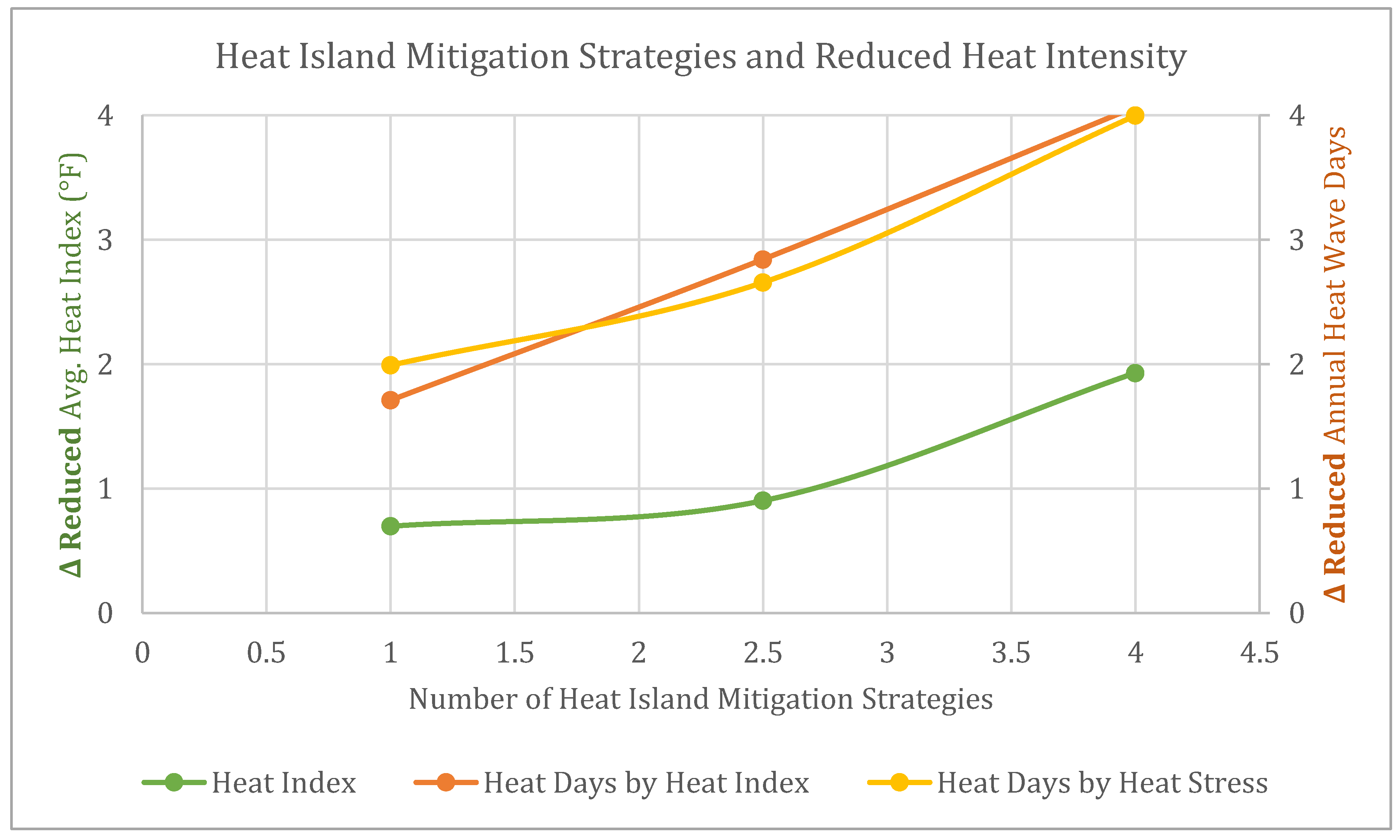
We find consistent results using a set of alternative specifications where the measure of heat hazard intensity used as an outcome variable is the number of heat wave days. The random trend model specification as described in Equation (3) with the alternative dependent variables is estimated. As shown in column (4) and (5), the estimation results suggest that counties with more heat island mitigation actions experience fewer heat wave days. For example, the Heat Wave Days decrease by 1.71 or 1.99 days on average (depending on the measure used to define the heat wave days) if a county initiates HIM activities by adopting a mitigation measure. The heat wave days further decrease as a county implements more HIM strategies; the difference between coefficients on 1 action group and 2-3 actions group dummies indicates that the reduction in heat wave days for additional measure is 0.67–1.13 days. The estimates suggest that the first HIM measure implemented in a county has the largest marginal effect (1.66–1.96), and the marginal effects of additional measures decrease, but still having a significant hazard-reduction effect. Figure 4 illustrates the heat-hazard lowering effect of heat island mitigation strategies using the results of specifications RTM_HI 3, RTM_HD 1 and 2.

5.2. Second-Phase: Heat Vulnerability–Fatality Model

Table 7. Heat vulnerability—fatalities model zero-inflated negative binomial regression results.

	Zero Inflated Negative Binomial Model (ZINB)
Dependent Variable	(1)	(2)	(3)	(4)
Direct Heat Fatalities	Specification 1	Specification 2	Specification 3	Specification 4
Monthly Avg. Max Heat Index (°F)	0.110 ***	0.110 ***	0.115 ***	0.110 ***
	(0.017)	(0.017)	(0.017)	(0.017)
Annual Avg. of Daily Temp. (°F)	−0.319 ***	−0.333 ***	−0.351 ***	−0.307 ***
	(0.104)	(0.098)	(0.108)	(0.098)
Annual Avg. of Max. Daily Temp. (°F)	0.220 **	0.230 ***	0.245 ***	0.206 **
	(0.087)	(0.084)	(0.090)	(0.083)
Ln (Population)	0.932 ***	0.927 ***	0.946 ***	0.953 ***
	(0.083)	(0.082)	(0.083)	(0.084)
Urban Population Density (per 1000 m2)	0.072 ***	0.067 ***	0.050 **	0.069 ***
	(0.022)	(0.021)	(0.020)	(0.020)
Percent Young	0.086 **	0.087 ***	0.074 **	0.083 **
	(0.034)	(0.033)	(0.033)	(0.033)
Percent Elderly	0.103 ***	0.094 ***	0.092 ***
	(0.027)	(0.028)	(0.028)
Percent Elderly Living Alone				0.292 ***
				(0.068)
Poverty Rate among Elderly			0.065 ***
			(0.021)
Poverty Rate		0.038 *
		(0.021)
Ln (Per Capita Income)	−1.003 *	−0.290	−0.146	−0.899
	(0.537)	(0.644)	(0.607)	(0.551)
Percent Non-White	0.016 ***	0.012 **	0.010 *	0.014 ***
	(0.005)	(0.006)	(0.006)	(0.005)
Percent Renter Occupied Housing	0.021 *	0.013	0.019	0.013
	(0.012)	(0.013)	(0.012)	(0.012)
Percent Mobile Homes	0.029 *	0.028 *	0.027	0.032 *
	(0.017)	(0.016)	(0.016)	(0.018)
Excessive Heat	0.001	0.012	0.007	−0.002
	(0.141)	(0.141)	(0.141)	(0.141)
State Fixed Effects	Yes	Yes	Yes	Yes
Time Effects	Yes	Yes	Yes	Yes
Observations	15,050	15,050	15,050	15,050

Notes: 1. Cluster (County)-adjusted Robust standard errors in parentheses, *** p < 0.01, ** p < 0.05, * p < 0.10; 2. The omitted category for the begin time is “Early Afternoon”; 3. The omitted category for the season is “Summer”; 4. The omitted category for event type is “Heat”; 5. The estimates of the constant term, state fixed effects, year effects, time of day indicator variables, and seasonal indicator variables are not reported here.

presents the estimates from the zero-inflated negative binomial models using heat events recorded at the scale of counties during the 1998–2011 period. The dependent variable is direct fatalities from each heat event. Because of the high correlation among the socio-economic variables, we estimate specification 1 as a base model and then introduce the poverty rate variable in specification 2, elderly poverty rate in specification 3 and percent elderly living alone in specification 4. Specifications 2 and 3 connect the issue of poverty and the resulting increase in heat vulnerability, whereas specifications 3 and 4 offer insight in the context of an aging society. The results from the first-stage inflation model (Logit) are available from the authors upon request.

5.2.1. Heat Hazard Profile

Consider now the results of the heat hazard profile variables. A measure of the intensity of a heat event, the heat index level, is found to be one of the most crucial meteorological elements of heat hazard that determines the level of societal impacts. The results from all four specifications demonstrate that a significant positive relationship holds between the heat index and heat-induced fatalities. An increase in the maximum daily heat index value by one degree (F) leads to 12% more heat fatalities, on average. The variables that signify the timing of the event are also estimated to affect the degree of heat impacts. The adverse impact of a heat event is greater when it begins to occur during late afternoon hours (4:00–7:59 p.m.), perhaps because higher temperatures at night in urban areas (because of the impeded release of heat absorbed during daytime in urban areas) may further increase nighttime atmospheric temperatures and exacerbate extreme heat impacts on human health.

5.2.2. Climatic and Environmental Conditions

Our estimates confirm that climatic and environmental characteristics of the place are also important determinants of heat vulnerability. The negative coefficient of the average daily air temperature suggests that counties in warmer climates tend to be less sensitive to heat as they are more likely accustomed to high temperatures. However, among counties with the same average temperature, those with the higher maximum daily temperatures may suffer greater heat-related fatalities. This result shows that susceptibility to heat hazards not only depends on an area’s normal climate conditions, but also on the meteorological variability (e.g., daily temperature range). Consistent with the previous heat study findings, the level of urbanization is an important heat risk factor. We find that more populated counties experience higher risk of life-threatening extreme heat. Also, urban concentration magnifies the risk aggravating heat island effects. The estimates imply that with a one standard deviation (SD) increase (≈2) in urban density (per 1000 m²), heat fatalities rise by 15%.

5.2.3. Demographic and Socio-Economic Characteristics

Our analysis provides statistically significant evidence of meaningful magnitudes in support of the “socio-political nature of disasters” framework—those who are more vulnerable in society are also more susceptible to harm from disaster events. First, we ascertain that demographic composition, such as the proportions of young and elderly population, and the proportion of non-white as essential factors that play a role in heat vulnerability. Of interest, age is a key factor where elderly people are more vulnerable to heat waves. Our heat vulnerability model estimates that a one percentage point increase in the share of the elderly population is associated with an 11% increase in heat fatalities (specification 1).

The relationship between heat vulnerability and the socially isolated elderly is also notable, as isolation increases physiological and societal vulnerabilities. The estimate in specification 4 indicates that a one-point increase in the proportion of the population that is elderly and isolated is associated with a 34% increase in heat-related fatalities. Greater heat vulnerability resulting from a growing share of socially isolated elderly is attributable to both the individual vulnerability of the elderly and the population characteristics of an aging society.

Estimates also show that racial groups experience differential heat impacts. Counties with a greater non-white population tend to have more heat-induced fatalities; a one standard deviation increase (≈16) in the share of the non-white population is correlated with 17–30% more heat fatalities, depending on the model specifications. Because vulnerability of certain race/ethnicity groups are highly linked with their socio-economic status [46], the estimated effect of the percent non-white variable decreases once we include poverty measures in specifications 2 and 3.

Overall, the results suggest that socio-economic factors are among several factors contributing to heat vulnerability. First, our estimates support the idea that higher economic status reduces vulnerability to extreme weather events, which has been echoed by other studies on disaster vulnerability. This relationship holds in the case of extreme heat, as well. Those with greater economic resources can utilize their wealth to prevent the worst consequences of and better respond to heat hazards. People living below the poverty line, on the other hand, are at a greater risk as they possess limited financial, physical, and social assets, which limits their coping capacity. A one percentage point increase in the poverty rate is associated with a 4% increase in fatalities, whereas a one standard deviation increase (≈7) is associated with 30% increase in fatalities.

A combination of two vulnerability factors—aging coupled with poverty—is considered in specification 3. For a one percentage point increase in senior poverty rates, heat fatalities are estimated to be 7% greater. Comparing with the estimated effect of a one-unit change in the overall poverty rate—4% increase in fatalities, we infer that among those who live in poverty, the elderly are much more susceptible to heat. Note that this is a partial effect because other variables—including the share of elderly population—are held constant.

To further investigate growing heat vulnerability resulting from an aging population, using the model estimate of specification 3 we calculate the future increase in heat fatalities. Before discussing the forecast further, we acknowledge that one should be cautious in interpreting the predicted increase in fatalities in

Table 8. Increase in heat fatalities given the projected growth of the elderly population in 2030 and 2040.

	Population aged 65+		65+ Population Growth		Yearly Heat Fatalities 2
Year	Share	Number 1	Δ Share	Δ Number 1	Pct Δ	Avg. Deaths/year	Δ Deaths
1998–2011	12.3%	35,945				142
2030	20.6%	73,138	8.3%	37,193	215%	305	163
2050	22.6%	85,675	10.3%	49,730	258%	366	224

Notes: ¹ Numbers in thousands; ² The predicted heat fatalities are calculated using the estimation result of the specification 3 in Table 7. Note that the predicted changes are average partial effects of the percent elderly variable, with all other variables being held constant.

as a causal effect considering the estimates from ZINB model (non-panel method; county heterogeneity not fully controlled for) may not necessarily reflect a causal relationship. We carry out this post-estimation exercise to provide a rough approximation of growing heat vulnerability in an aging society based on the projected growth of the elderly population and elderly poverty rates: (i) The national share of elderly in the population during our study period is 12.3% (12.3% is the national level statistic while our sample mean of 14.94% in Table 5 is the mean of county level Pct Elderly, where some counties are included multiple times for the computation of the mean value.) (a 14-year average) and is projected to rise to 20.6% by 2030 and 22.6% by 2050 [62]; and (ii) 1 out of 10 elderly lived in poverty during 1990–2014 (10.34%, 25 year average) [63]. The population projections indicate that the share of elderly will rise by 8.3 percentage points by 2030 and 10.3 percentage points by 2050. Using these statistics, the predicted increase in heat fatalities for years 2030 and 2050 are calculated using the coefficient estimates from specification 3 as reported in Table 7, assuming the poverty rates among elderly will remain the same at the average rate of 10.34% in 2030 and 2050. We are primarily interested in the projected increase in heat fatalities in relation with the growth in elderly in this calculation while considering the poverty rates among the elderly. However, because of the assumption of ceteris paribus of multiple regression analysis, the coefficient of Pct Elderly in specification 3 is a partial effect of the increase in Pct Elderly, holding other variables including the elderly poverty rate constant. Assuming the poverty rates among the elderly will remain the same, we estimate the predicted increase in heat fatalities as a result of the aging population using the estimates from specification 3.

As shown in Table 8, we find that the heightened heat vulnerability due to the growth of the elderly population may result in a two-fold increase in heat fatalities by 2030 and about 2.6-fold increase by 2040, relative to the average fatalities during our study period (1998–2011). Heat vulnerability in the USA is predicted to increase substantially in the coming decades as the most heat-vulnerable group of people (the elderly) is a growing share of the population.

Consider next the housing-related factors where the results show that housing ownership is closely related with heat vulnerability. A one standard deviation increase (≈8) in the share of renter occupied housing is associated with a 16% increase in heat fatalities (specification 3). Also, consistent with the previous findings on the vulnerability of those living in mobile homes [33,34,41], our analysis shows that living in mobile homes are a significant heat risk factor. For a one standard deviation increase (≈9) in the share of mobile homes in the total housing stock, heat fatalities are estimated to be 26% larger. It may be that increased vulnerability of those living in mobile homes (particularly older mobile homes) is the result of lower quality relative to traditional homes in terms of cooling systems and/or insufficient insulation and windows. These results also further highlight greater vulnerability of those who have limited financial resources and may have no other choice but to live in lower cost rental housing or mobile homes.

5.3. Heat Island Mitigation Actions and Heat Fatality

5.3.1. First and Second Phase Models Combined: A Mediated Effect

As illustrated in Section 4, we combine the results from the first-phase heat index model (Equation (4)) with the second-phase estimation results of the heat fatality analysis (Equation (5)) to derive a mediated effect of heat mitigation actions on heat fatalities. Using the estimated coefficients from three specifications (columns 1, 2, 3) in Table 6 and the coefficient on the heat index variable from specification 2 in Table 7, we compute the mediated effects on heat fatalities as presented in

Table 9. The mediated effect of heat mitigation measures on heat fatalities.

Model		Variables	Estimates	Effects on Heat Fatalities
Heat Fatality Model		Monthly Avg. Max Heat Index (°F)	${\widehat{\delta }}_1$ = +0.110 ***	$(1-\exp ({\widehat{\delta }}_1·{\widehat{\beta }}_1)) \%$
Heat Hazard Model	1	Heat Island Mitigation (HIM) Adoption Status 1	${\widehat{\beta }}_{1d}$ = −0.710 ***	7.51% Reduction 1
	2	No. of HIM Measures	${\widehat{\beta }}_{1n}$ = −0.261 ***	2.83% Reduction (for one additional action)
	3	1 Mitigation Actions Group 1	${\widehat{\beta }}_{11}$ = −0.698 ***	7.39% Reduction 1
		2–3 Mitigation Actions Group 1	${\widehat{\beta }}_{12}$ = −0.903 ***	9.46% Reduction 1
		+4 Mitigation Actions Group 1	${\widehat{\beta }}_{13}$ = −1.930 ***	19.13% Reduction 1

Notes: ¹ The reference group for these group indicator variables is non-adoption (zero-actions) group; ² *** means p-values <0.01.

.

Before discussing the findings, on caveat is in order: Even though our findings provide evidence on the negative causality between the heat mitigation measures and the heat fatalities, one should be cautious in interpreting the magnitude of the effects. The estimates indicate that counties in the heat island mitigation adoption group experience an average of 7.51% fewer heat fatalities than those in non-adoption group. Also, one additional heat reduction measure reduces heat fatalities by 2.8%, on average. However, because of the long-lasting and synergistic effects of the heat mitigation measures, the temperature lowering benefit of such measures accumulate and thus, counties with more mitigation actions are progressively less vulnerable to extreme heat than counties with fewer actions. As shown in the lowest panel of Table 9, counties in the 1 action group suffer 7.39% fewer heat fatalities, compared to the non-adoption counties, whereas counties in that 2–3 actions group experience 9.46% fewer heat fatalities. The fatality reducing effects increase progressively as a county adopts 4 or more heat mitigation actions. The mediated effect analysis shows that counties in 4+ actions group avoid many heat event fatalities as result of their mitigation efforts. This evaluation suggests that heat fatalities are reduced by 19% as compared to the non-adoption group.

5.3.2. A Direct Estimation of the Effect

We also perform a direct estimation of the effect of heat island mitigation (HIM) measures on heat fatalities, using the Poisson fixed effects estimator, controlling for the unobserved heterogeneity of counties as well as year effects. We use county-year panel structured data with deaths per heat event as the dependent variable. In Section 5.1, the HIM measures are found to have significant heat lowering effects. In Section 5.2, using the heat index as an intermediary variable, we show that HIM measures influence the heat outcomes. Focusing on the identification of the effect of heat mitigation efforts on fatalities, we only include the HIM variables as a regressor along with controls, excluding the intermediary variable—the heat index measure. However, it is still important to capture the changes in heat fatalities due to the naturally occurring variation in heat over the period that might not be explained by other climatic variables nor by the HIM variable. Thus, we include the days in which the county max air temperature (the heat days measure is closely related with the heat index, but it only accounts for the temperature component of extreme heat and not the humidity component) reached or exceeded the 95th percentile of daily max temperature during the May–September period, along with other meteorological conditions.

The results of the direct estimation of the effects of HIM actions on heat fatalities using the Poisson fixed effects estimation method are presented in columns (1)–(2) of

Table 10. A direct estimation of the effect of heat island mitigation (HIM) actions on heat fatalities–Poisson fixed (FE) and random (RE) effects model key results.

Dependent Variable	(1)	(2)	(3)	(4)
Direct Heat Fatalities	Poisson FE	Poisson RE	Poisson FE	Poisson RE
No. of HIM Actions_lag (All)	−0.052	−0.107 *
	(0.068)	(0.064)
No. of HIM Actions_lag_(Non-Statewide)			−0.161 ***	−0.169 **
			(0.060)	(0.066)
Previous-3yrs_HeatWaveDays	−0.057 ***	−0.047 ***	−0.057 ***	−0.047 ***
	(0.018)	(0.016)	(0.018)	(0.016)
Heat Wave Days (based on Max Temp)	0.017 *	0.009	0.017 *	0.010
	(0.010)	(0.008)	(0.009)	(0.008)
Population (in thousands)	0.001	0.001 ***	0.001	0.001 ***
	(0.001)	(0.000)	(0.002)	(0.000)
Pct Urban Population	0.041	0.028 ***	0.030	0.028 ***
	(0.051)	(0.006)	(0.050)	(0.006)
Ln (Per Capita Income)	−2.202	−1.477 **	−3.195	−1.491 **
	(3.025)	(0.587)	(2.971)	(0.590)
Number of Counties	260	1906	260	1906
Observations	1519	6635	1519	6635

Notes: 1. Cluster (County)-adjusted Robust standard errors in parentheses, *** p < 0.01, ** p < 0.05, * p < 0.10; 2. The estimates of meteorological, demographic control variables, the constant term, and time fixed effects are not reported here; 3. The number of counties with any heat occurrence during the study period is 1906 (random effect estimation). However, the number of counties with any heat fatality during the period is 260 (fixed effects estimation).

. The random effects model results are provided in columns (3)–(4) as a robustness check. We find a statistically significant evidence that the more HIM measures a county has implemented, the smaller the heat fatalities in that county. However, the difference between the estimated effects of the number of all HIM measures shown in column (2) and the effects of the number of locally implemented measures (i.e., non-statewide activities) in column (3) implies that the heat-vulnerability reducing benefits of HIM activities can differ depending on the spatial-scale and the main agents of HIM implementation. The results indicate that community-based local government initiated HIM actions have larger fatality reducing effects. This result suggests adaptation plans and interventions that are tailored to each targeted area and established with knowledge on unique circumstances of localities is important. An additional heat island mitigation measure that is locally implemented in a county is estimated to reduce the annual deaths rate (deaths per heat event) by 14.87%. However, note that the estimated direct effect is much larger than the mediated effect that is identified in Table 9. This might be partly due to the differences in estimators—cross-sectional method (ZINB) vs. within-estimator (FE) where the latter is preferable in causal inferences. Also, the incongruent data structures of the first- and second-phase models and the different measures for the heat intensity variable in the two phases—annual max. HI vs. monthly max. HI—likely contribute to the difference in the mediated versus direct effects.

5.4. Falsification Tests

We also perform falsification tests on the significant effects of HIM measures estimated in the first-phase heat hazard mitigation model and in the direct estimation of fatality-reducing effect of the HIM measures. Our falsification tests use the baseline specifications, except that we include the 2-year-lead heat island mitigation variables instead of the 2-year lagged variables in the baseline regressions. This test is performed to verify that the estimated effects are not driven by characteristics common to counties that are about to employ heat mitigation measures.

The falsification test results of the first-phase heat hazard model are available from the authors upon request. Once the 2-year-lead HIM variables are used, the cooling-effects of HIM measures disappear. Test results of other specifications with different heat intensity measures, such as annual heat wave days by maximum heat index or heat wave days by net daily heat stress are also consistent. The positive coefficients may be capturing the inverse relationship between heat hazard (=heat intensities) and the proactive adaptation measures to mitigate the risk of heat (=HIM). The higher the heat intensity within a community is, the more likely it is for a community to take heat risk mitigation actions.

Similarly, the falsification test results of the direct estimation of the effects of HIM actions on heat fatalities, which are also available from the authors upon request, rule out the possibility that our results are spurious. Compared to the statistically significant, negative estimates of lagged HIM measures from the baseline regressions in Table 10, lead variables reverse the previous results, losing statistical significance in all specifications.

6. Conclusions

Under ongoing climate change, the frequency and intensity of extreme heat events are predicted to increase. Given the devastating consequences of heat events and the growing risk of extreme heat, it is critical to identify the major determinants of heat vulnerability to minimize potential human losses. Our analysis reveals the multi-faceted nature of the heat vulnerability; event-specific heat hazard profiles, meteorological, climatic, and environmental conditions, as well as various socio-economic and housing factors all play a role in determining heat vulnerability. Findings suggest that current societal issues such as the aging population, continuing urbanization, and deepening poverty and inequality that seem to be unrelated to natural disasters, are contributing factors to the growing extreme heat vulnerability in the USA Of special interest is the aging population combined with the projected increase in heat risks, which is expected to aggravate the adverse consequences of extreme heat. According to our estimates, increasing heat vulnerability due to the growth of the elderly population is predicted to generate a two-fold increase in heat-induced fatalities by 2030; public heat island mitigation efforts are more important than ever. This study provides evidence of the benefits of community heat island mitigation measures in reducing heat risk and associated fatalities. Our findings underscore the need for more proactive and precautionary public measures to counteract the harmful effects of heat hazards. In this regard, a key area of additional research is to conduct further analyses to examine which of the heat island mitigation strategies are most effective and which have the highest net societal benefits. Further study along these lines would provide useful information for community decisions regarding heat island mitigation measures. Overall, findings of this study inform targeting efforts designed to protect and assist the most vulnerable population subgroups and guide future policies and mitigation efforts to counteract the growing risk of heat waves at the local, state and national levels.

References

- Kochanek, K.D.; Miniño, A.M.; Murphy, S.L.; Xu, J.; Kung, H.-C. Deaths: Final Data for 2009. 2011. Available online: https://stacks.cdc.gov/view/cdc/12124 (accessed on 8 March 2018).
- Greenough, G.; McGeehin, M.; Bernard, S.M.; Trtanj, J.; Riad, J.; Engelberg, D. The potential impacts of climate variability and change on health impacts of extreme weather events in the United States. Environ. Health Perspect. 2001, 109, 191–198. [Google Scholar]
- Beniston, M.; Stephenson, D.B. Extreme climatic events and their evolution under changing climatic conditions. Glob. Planet. Chang. 2004, 44, 1–9. [Google Scholar] [CrossRef] [Green Version]
- Meehl, G.A.; Tebaldi, C. More intense, more frequent, and longer lasting heat waves in the 21st century. Science 2004, 305, 994–997. [Google Scholar] [CrossRef] [PubMed] [Green Version]
- Milly, P.C.D.; Wetherald, R.T.; Dunne, K.A.; Delworth, T.L. Increasing risk of great floods in a changing climate. Nature 2002, 415, 514–517. [Google Scholar] [CrossRef] [PubMed]
- Stocker, T.F.; Qin, D.; Plattner, G.K.; Tignor, M.; Allen, S.K.; Boschung, J.; Nauels, A.; Xia, Y.; Bex, V.; Midgley, P.M. IPCC, 2013: Summary for Policymakers in Climate Change 2013: The Physical Science Basis, Contribution of Working Group I to the Fifth Assessment Report of the Intergovernmental Panel on Climate Change; Cambridge University Press: Cambridge, UK, 2013. [Google Scholar]
- Strader, S.M.; Ashley, W.S.; Pingel, T.J.; Krmenec, A.J. Projected 21st century changes in tornado exposure, risk, and disaster potential. Clim. Chang. 2017, 141, 301–313. [Google Scholar] [CrossRef]
- Deschênes, O.; Greenstone, M. Climate Change, Mortality, and Adaptation: Evidence from Annual Fluctuations in Weather in the US. Am. Econ. J. Appl. Econ. 2011, 3, 152–185. [Google Scholar] [CrossRef]
- Morss, R.E.; Wilhelmi, O.V.; Meehl, G.A.; Dilling, L. Improving Societal Outcomes of Extreme Weather in a Changing Climate: An Integrated Perspective. Annu. Rev. Environ. Resour. 2011, 36, 1–25. [Google Scholar] [CrossRef] [Green Version]
- Gago, E.J.; Roldan, J.; Pacheco-Torres, R.; Ordóñez, J. The city and urban heat islands: A review of strategies to mitigate adverse effects. Renew. Sustain. Energy Rev. 2013, 25, 749–758. [Google Scholar] [CrossRef]
- U.S. Environmental Protection Agency (EPA). Reducing Urban Heat Islands: Compendium of Strategies Draft; U.S. Environmental Protection Agency (EPA): Washington, DC, USA, 2008.
- Hondula, D.M.; Davis, R.E.; Leisten, M.J.; Saha, M.V.; Veazey, L.M.; Wegner, C.R. Fine-scale spatial variability of heat-related mortality in Philadelphia County, USA, from 1983–2008: A case-series analysis. Environ. Health 2012, 11, 16. [Google Scholar] [CrossRef] [Green Version]
- Sheridan, S.C.; Dolney, T.J. Heat, mortality, and level of urbanization: Measuring vulnerability across Ohio, USA. Clim. Res. 2003, 24, 255–265. [Google Scholar] [CrossRef] [Green Version]
- Uejio, C.K.; Wilhelmi, O.V.; Golden, J.S.; Mills, D.M.; Gulino, S.P.; Samenow, J.P. Intra-urban societal vulnerability to extreme heat: The role of heat exposure and the built environment, socioeconomics, and neighborhood stability. Health Place 2011, 17, 498–507. [Google Scholar] [CrossRef]
- Bell, M.L.; O’neill, M.S.; Ranjit, N.; Borja-Aburto, V.H.; Cifuentes, L.A.; Gouveia, N.C. Vulnerability to heat-related mortality in Latin America: A case-crossover study in Sao Paulo, Brazil, Santiago, Chile and Mexico City, Mexico. Int. J. Epidemiol. 2008, 37, 796–804. [Google Scholar] [CrossRef] [PubMed] [Green Version]
- Loughnan, M.; Tapper, N.; Phan, T. Identifying Vulnerable Populations in Subtropical Brisbane, Australia: A Guide for Heatwave Preparedness and Health Promotion. Int. Sch. Res. Not. 2014, 2014, e821759. [Google Scholar] [CrossRef] [Green Version]
- Stafoggia, M.; Forastiere, F.; Agostini, D.; Biggeri, A.; Bisanti, L.; Cadum, E.; Caranci, N.; de’Donato, F.; De Lisio, S.; De Maria, M.; et al. Vulnerability to heat-related mortality: A multicity, population-based, case-crossover analysis. Epidemiology 2006, 17, 315–323. [Google Scholar] [CrossRef] [PubMed]
- Klinenberg, E. Denaturalizing Disaster: A Social Autopsy of the 1995 Chicago Heat Wave. Theory Soc. 1999, 28, 239–295. [Google Scholar] [CrossRef]
- Browning, C.R.; Wallace, D.; Feinberg, S.L.; Cagney, K.A. Neighborhood social processes, physical conditions, and disaster-related mortality: The case of the 1995 Chicago heat wave. Am. Sociol. Rev. 2006, 71, 661–678. [Google Scholar] [CrossRef] [Green Version]
- Aubrecht, C.; Özceylan, D. Identification of heat risk patterns in the U.S. National Capital Region by integrating heat stress and related vulnerability. Environ. Int. 2013, 56, 65–77. [Google Scholar] [CrossRef]
- Harlan, S.L.; Declet-Barreto, J.H.; Stefanov, W.L.; Petitti, D.B. Neighborhood Effects on Heat Deaths: Social and Environmental Predictors of Vulnerability in Maricopa County, Arizona. Environ. Health Perspect. (Online) Res. Triangle Park 2013, 121, 197. [Google Scholar] [CrossRef] [Green Version]
- Johnson, D.P.; Stanforth, A.; Lulla, V.; Luber, G. Developing an applied extreme heat vulnerability index utilizing socioeconomic and environmental data. Appl. Geogr. 2012, 35, 23–31. [Google Scholar] [CrossRef]
- Reid, C.E.; O’Neill, M.S.; Gronlund, C.J.; Brines, S.J.; Brown, D.G.; Diez-Roux, A.V.; Schwartz, J. Mapping community determinants of heat vulnerability. Environ. Health Perspect. 2009, 117, 1730. [Google Scholar] [CrossRef]
- North America Land Data Assimilation System (NLDAS). Daily Air Temperatures and Heat Index, years 1979–2011 on CDC WONDER Online Database. Available online: http://wonder.cdc.gov/NCA-heatwavedays-historic.html (accessed on 11 January 2018).
- Albala-Bertrand, J.M. Political Economy of Large Natural Disasters; Oxford University Press: New York, NY, USA, 1993. [Google Scholar]
- Blaikie, P.; Canon, T.; Davis, I.; Wisner, B. At risk: Natural Hazards, People’s Vulnerability, and Disasters; Routledge: New York, NY, USA, 1994. [Google Scholar]
- Cutter, S.L. The landscape of disaster resilience indicators in the USA. Nat. Hazards 2016, 80, 741–758. [Google Scholar] [CrossRef]
- Enarson, E.; Morrow, B.H. The Gendered Terrain of Disaster: Through Womens Eyes; International Hurricane Center, Praeger Publishers: Westport, CT, USA, 1998. [Google Scholar]
- Peacock, W.G.; Morrow, B.H.; Gladwin, H. Hurricane Andrew: Ethnicity, Gender, and the Sociology of Disasters; Routledge: New York, NY, USA, 1997. [Google Scholar]
- Morrow, B.H. Identifying and Mapping Community Vulnerability. Disasters 1999, 23, 1–18. [Google Scholar] [CrossRef] [PubMed]
- Brooks, N.; Adger, W.N.; Kelly, P.M. The Determinants of Vulnerability and Adaptive Capacity at the National Level and the Implications for Adaptation. Glob. Environ. Chang. Adapt. Clim. Chang. Perspect. Across Scales 2005, 15, 151–163. [Google Scholar] [CrossRef]
- Donner, W.R. The political ecology of disaster: An analysis of factors influencing U.S. tornado fatalities and injuries, 1998–2000. Demography 2007, 44, 669–685. [Google Scholar] [CrossRef]
- Lim, J.; Loveridge, S.; Shupp, R.; Skidmore, M. Double Danger in the Double Wide: Dimensions of Poverty, Housing Quality and Tornado Impacts. Reg. Sci. Urban Econ. 2017, 65, 1–15. [Google Scholar] [CrossRef]
- Lim, J.; Skidmore, M. Flood Fatalities in the United States: The Roles of Socio-Economic Factors and the National Flood Insurance Program. South. Econ. J. 2019, 85, 1032–1057. [Google Scholar] [CrossRef]
- Zahran, S.; Brody, S.D.; Peacock, W.G.; Vedlitz, A.; Grover, H. Social Vulnerability and the Natural and Built Environment: A Model of Flood Casualties in Texas. Disasters 2008, 32, 537–560. [Google Scholar] [CrossRef]
- Kahn, M.E. The Death Toll from Natural Disasters: The Role of Income, Geography, and Institutions. Rev. Econ. Stat. 2005, 87, 271–284. [Google Scholar] [CrossRef]
- Toya, H.; Skidmore, M. Economic development and the impacts of natural disasters. Econ. Lett. 2007, 94, 20–25. [Google Scholar] [CrossRef]
- Strömberg, D. Natural Disasters, Economic Development, and Humanitarian Aid. J. Econ. Perspect. 2007, 21, 199–222. [Google Scholar] [CrossRef]
- Kellenberg, D.K.; Mobarak, A.M. Does rising income increase or decrease damage risk from natural disasters? J. Urban Econ. 2008, 63, 788–802. [Google Scholar] [CrossRef]
- Raschky, P.A. Institutions and the Losses from Natural Disasters. Nat. Hazards Earth Syst. Sci. 2008, 8, 627–634. [Google Scholar] [CrossRef]
- Simmons, K.M.; Sutter, D. The Economic and Societal Impact of Tornadoes; Springer Science & Business Media: Berlin/Heidelberg, Germany, 2011. [Google Scholar]
- Hajat, S.; Kosatky, T. Heat-Related Mortality: A Review and Exploration of Heterogeneity. J. Epidemiol. Community Health 2010, 64, 753–760. [Google Scholar] [CrossRef] [PubMed]
- Åström, D.O.; Bertil, F.; Joacim, R. Heat wave impact on morbidity and mortality in the elderly population: A review of recent studies. Maturitas 2011, 69, 99–105. [Google Scholar] [CrossRef]
- Kovats, R.S.; Hajat, S. Heat Stress and Public Health: A Critical Review. Annu. Rev. Public Health 2008, 29, 41–55. [Google Scholar] [CrossRef] [PubMed]
- Fothergill, A.; Maestas, E.G.; Darlington, J.D. Race, ethnicity and disasters in the United States: A review of the literature. Disasters 1999, 23, 156–173. [Google Scholar] [CrossRef]
- Hansen, A.; Bi, L.; Saniotis, A.; Nitschke, M. Vulnerability to Extreme Heat and Climate Change: Is Ethnicity a Factor? Glob. Health Action 2013, 6, 21364. [Google Scholar] [CrossRef] [PubMed] [Green Version]
- Lal, P.N.; Lal, P.N.; Singh, R.; Holland, P. Relationship between Natural Disasters and Poverty: A Fiji Case Study; SOPAC: Suva, Fiji, 2009. [Google Scholar]
- Fothergill, A.; Peek, L.A. Poverty and Disasters in the United States: A Review of Recent Sociological Findings. Nat. Hazards 2004, 32, 89–110. [Google Scholar] [CrossRef]
- Aptekar, L. The Psychosocial Process of Adjusting to Natural Disasters; Natural Hazards Research and Applications Information Center, University of Colorado: Boulder, CO, USA, 1991. [Google Scholar]
- Phillips, B.D. Cultural diversity in disasters: Sheltering, housing, and long-term recovery. Int. J. Mass Emerg. Disasters 1993, 11, 99–110. [Google Scholar]
- Pastor, M.; Bullard, R.D.; Boyce, J.K.; Fothergill, A.; Morello-Frosch, R.; Wright, B. In the Wake of the Storm: Environment, Disaster and Race after Katrina; Russell Sage Foundation: New York, NY, USA, 2006. [Google Scholar]
- Cutter, S.L.; Boruff, B.J.; Shirley, W.L. Social Vulnerability to Environmental Hazards*. Soc. Sci. Q. 2003, 84, 242–261. [Google Scholar] [CrossRef]
- Rosenzweig, C.; Solecki, W.D.; Cox, J.; Hodges, S.; Parshall, L.; Lynn, B.; Goldberg, R.; Gaffin, S.; Slosberg, R.B.; Savio, P. Mitigating New York City’s Heat Island: Integrating Stakeholder Perspectives and Scientific Evaluation. Bull. Am. Meteorol. Soc. 2009, 90, 1297–1312. [Google Scholar] [CrossRef]
- Synnefa, A.; Dandou, A.; Santamouris, M.; Tombrou, M.; Soulakellis, N. On the Use of Cool Materials as a Heat Island Mitigation Strategy. J. Appl. Meteorol. Climatol. 2008, 47, 2846–2856. [Google Scholar] [CrossRef]
- Perini, K.; Magliocco, A. Effects of Vegetation, Urban Density, Building Height, and Atmospheric Conditions on Local Temperatures and Thermal Comfort. Urban. For. Urban Green. 2014, 13, 495–506. [Google Scholar] [CrossRef]
- Tan, Z.; Lau, K.K.-L.; Ng, E. Urban Tree Design Approaches for Mitigating Daytime Urban Heat Island Effects in a High-Density Urban Environment. Energy Build. 2016, 114, 265–274. [Google Scholar] [CrossRef]
- Akbari, H.; Pomerantz, M.; Taha, H. Cool Surfaces and Shade Trees to Reduce Energy Use and Improve Air Quality in Urban Areas. Sol. Energy Urban. Environ. 2001, 70, 295–310. [Google Scholar] [CrossRef]
- Center for Disease Control and Prevention National Climate Assessment-Extreme Heat Events: Heat Wave Days in May-September for years 1981–2010 on CDC WONDER Online Database. Available online: http://wonder.cdc.gov/NCA-heatwavedays-historic.html (accessed on 15 January 2018).
- Wooldridge, J.M. Econometric Analysis of Cross Section and Panel Data; MIT Press: Cambridge, MA, USA, 2010; ISBN 978-0-262-29679-3. [Google Scholar]
- Long, J.S.; Freese, J. Regression Models for Categorical Dependent Variables Using Stata; Stata Press: College Station, TX, USA, 2006. [Google Scholar]
- Wooldridge, J.M. Specification testing and quasi-maximum-likelihood estimation. J. Econom. 1991, 48, 29–55. [Google Scholar] [CrossRef] [Green Version]
- U.S. Census Bureau. Projected Age Groups and Sex. Composition of the Population: Main Projections Series for the United States, 2017–2060; U.S. Census Bureau, Population Division: Washington, DC, USA, 2017.
- U.S. Census Bureau. 65+ in the United States: 2010; U.S. Government Printing Office: Washington, DC, USA, 2014.
Figure 1.
Summertime average maximum heat index vs. daily maximum temperature (1998–2011). Authors’ own illustration. Data: NLDAS Daily Air Temperatures and Heat Index, CDC [24].
Figure 2.
Total number of heat waves and yearly heat-induced fatalities by state (1996–2015). Source: Authors’ own illustration. Data: National Centers for Environmental Information (NCEI).
Figure 3.
Conceptualizing multi-faceted heat vulnerability. Source: Authors’ own illustration.
Figure 4.
The heat-hazard-lowering effects of heat island mitigation strategies.