The Buttressed Walls Problem: An Application of a Hybrid Clustering Particle Swarm Optimization Algorithm

Abstract

The design of reinforced earth retaining walls is a combinatorial optimization problem of interest due to practical applications regarding the cost savings involved in the design and the optimization in the amount of CO${}_2$ emissions generated in its construction. On the other hand, this problem presents important challenges in computational complexity since it involves 32 design variables; therefore we have in the order of ${10}^{20}$ possible combinations. In this article, we propose a hybrid algorithm in which the particle swarm optimization method is integrated that solves optimization problems in continuous spaces with the db-scan clustering technique, with the aim of addressing the combinatorial problem of the design of reinforced earth retaining walls. This algorithm optimizes two objective functions: the carbon emissions embedded and the economic cost of reinforced concrete walls. To assess the contribution of the db-scan operator in the optimization process, a random operator was designed. The best solutions, the averages, and the interquartile ranges of the obtained distributions are compared. The db-scan algorithm was then compared with a hybrid version that uses k-means as the discretization method and with a discrete implementation of the harmony search algorithm. The results indicate that the db-scan operator significantly improves the quality of the solutions and that the proposed metaheuristic shows competitive results with respect to the harmony search algorithm.

1. Introduction

Retaining walls are structures widely used in engineering for supporting soil laterally. The design of these walls is a problem of interaction between the soil and the structure to retain a material safely and economically. When the height of a cantilever wall becomes important, the volume of concrete required begins to be considerable. From a height of 8–10 m, buttressed walls economize its design. The design of these structures is mainly carried out following rules very much linked to the experience of structural engineers [1]. If the initial design dimensions or material qualities are inadequate, the structure is redefined. With this procedure of trial and error, the different designs obtained do not go beyond a few tests. This process leads to a safe, but not necessarily economic, design [2]. Structural optimization methods have clear advantages over experience-based design.

Presently, the optimum design of reinforced concrete (RC) structures constitutes a relevant line of research. In practical structural optimization problems, the variables used must be discrete, so they are combinatorial optimization problems. However, combinatorial problems are found in a large number of real problems such as allocation resources [3,4], logistics [5], transport [6], routing problems [7,8], scheduling problems [6,9], and engineering design projects [10,11], among others. These problems present a space of solutions that grows exponentially with the variables used, so the metaheuristics, which were inspired by natural phenomena for continuous spaces, are a good approach to obtain optimum solutions to engineering problems. However, two important characteristics of metaheuristics, intensification and diversification, must be preserved to design discrete versions of these algorithms.

While structural optimization began by minimizing the weight or cost of structures [12,13], other objective functions related to the social, Reference [14] and environmental sustainability of structures [15] throughout their entire life cycle have subsequently been incorporated. Reducing the carbon footprint of RC structures is currently investigated as an optimization target. In particular, a hybrid multistart optimization strategic method based on a variable neighborhood search threshold acceptance strategy [16] was used to reduce the cost and carbon-emissions in cantilever retaining walls. A hybrid harmony search together with a threshold acceptance strategy [17,18], the black hole algorithm [17] and a hybrid k-means cuckoo search algorithms [10] were applied to minimize both the economic cost and the CO${}_2$ emissions in counterfort retaining walls. A CO${}_2$ and cost analysis in precast–prestressed concrete road bridges was developed in [15]. In [14], the importance of the criteria that define social sustainability was analyzed. These criteria considered the complete life of infrastructure. The social sustainability of infrastructure projects was tackled in [14] using Bayesian methods. In recent works [19,20], different meta-heuristics algorithms were used for optimal design of RC retaining walls. The life cycle assessment of earth-retaining walls was analyzed in [21,22].

A strategy that reinforces the results obtained by the metaheuristics has been the hybridization with techniques that deeply modify their way of working. Hybridization is carried out in different ways, the most important of which are: (i) mathematics, integrating mathematical programming and metaheuristics [23], (ii) hybrid heuristics, combining different metaheuristics [24], (iii) symmetrical heuristics, where simulation and metaheuristics are combined [25], and (iv) hybridization between metaheuristics and machine learning.

In this article, we used an emerging line of research that integrates the areas of machine learning and metaheuristic algorithms with the goal of tackle the design of reinforced earth retaining walls problem. This problem presents important challenges in computational complexity since it involves 32 design variables, therefore we have on the order of ${10}^{20}$ possible combinations. Therefore, it is interesting to understand how these types of hybrid techniques perform in this problem, in addition to comparing these ones with the state-of-the-art solutions that addressed the design of this type of walls.

The proposed hybrid algorithm uses a machine learning algorithm in a discrete operator that allows continuous metaheuristics to tackle combinatorial optimization problems. In this way, a combinatorial optimization problem, such as the buttressed wall design, can be addressed. The contributions of this work are as follows:

• A hybrid Particle Swarm Optimization (PSO) based on a db-scan clustering technique is proposed. The db-scan is very effective in binary combinatorial problems [6,10]. PSO is often used to solve continuous optimization problems and its tuning is very simple.
• The contribution of the db-scan in the discretization process was studied through a random operator. In addition, the discretization performed by db-scan was compared with methods using k-means [5,26].
• The proposed algorithm is applied to obtain low-carbon, low-cost counterfort wall designs. This hybrid algorithm is compared with an efficient algorithm adapted from the harmony search (HS) proposed in [18].

The rest of this paper is structured as follows: in Section 2 we develop a state-of-the-art of hybridizing metaheuristics with machine learning; in Section 3 we define the optimization problem, the variables involved, and the restrictions; then in Section 4 we detail the discrete db-scan algorithm; we move on with the experiments and results obtained in Section 5; and conclude with Section 6 in which we summarize the conclusions and new lines of research.

2. Hybridizing Metaheuristics with Machine Learning

Metaheuristics is a broad collection of incomplete optimization techniques inspired by some real-world phenomenon in nature or in the behavior of living beings [27,28]. The objective is to solve problems of high computational complexity in a reasonable execution time so that its optimization mechanism is not significantly affected when the problem to be solved is altered. Then again, the set of techniques capable of learning from a database are the so-called machine learning algorithms [29]. Depending on the learning mode, these techniques are divided into learning by reinforcement, supervised learning, and unsupervised learning. It is common for these algorithms to be used in a wide range of problems such as regression, dimensionality reduction, transformation, classification, time series or anomaly detection and computer vision problems.

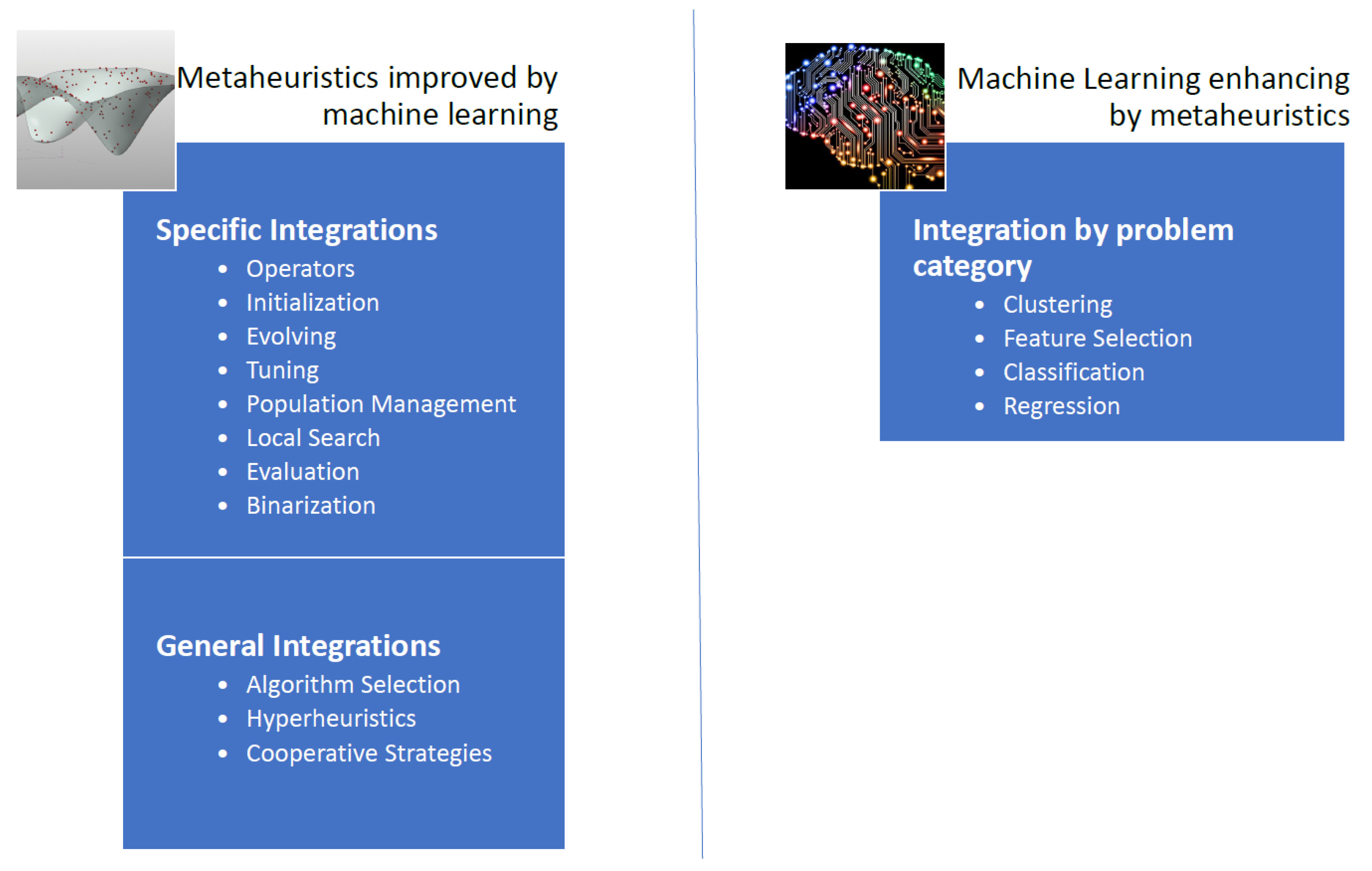
The integration of the machine learning techniques with the metaheuristic algorithms can be done basically with two approaches [30]. Either machine learning techniques are used to increase the quality of the solutions and the convergence rates obtained by metaheuristics, or metaheuristic are used to enhance the performance of machine learning techniques [30]. However, metaheuristics often improves the efficiency of an optimization problem concerning machine learning. Based on the work of [30], we propose an extension of the scheme of techniques in which metaheuristics and machine learning are combined (Figure 1).

Machine learning can be used as a metamodel to determine from a set of metaheuristics the best one for each instance. In addition, specific machine learning operators can also be embedded into a metaheuristic, resulting in three different groups of techniques: hyper-heuristics, algorithm selection, and cooperative strategies [30].

If we automate the design and tuning of metaheuristics to solve a large number of problems, we obtain the so-called hyper-heuristics. The aim of the cooperation strategies is to obtain methods that are more robust by combining the algorithms in a parallel or sequential way. The cooperation mechanism can share the whole solution, or only a part of it. In [31], a multi-objective optimization of an aerogel glazing system through a surrogate model driven by the cross-entropy function was developed with the implementation of the supervised machine-learning method. In [32] the multilevel thresholding image segmentation-based hyperheuristic method was addressed. Finally, in [33] an agent-based distributed framework was proposed to solve the problem of permutation flow stores, and in which each agent is implementing a different metaheuristic.

On the other hand, there are operators that allow enhancing the performance of a metaheuristic integrating machine learning operators. Initialization, population management, solution disruption, binaryization, local search operators and parameter setting and are examples of such operators [30]. Binary operators using unsupervised learning techniques can be integrated into metaheuristics that operate in continuous spaces to perform the binarization process [6]. In [34], a percentile transition-ranking algorithm was proposed as a mechanism to binarize continuous metaheuristics. In [9], the application of Big Data techniques was applied to improve a cuckoo search binary algorithm. The tuning of the parameters of metaheuristics is another line of research of interest. In [35], a tuning method was applied on different sized problem sets for the real-world integration and test order problem. In [36] a semi-automatic approach designs the fuzzy logic rule base to obtain instance-specific parameter values using decision trees. The use of machine learning techniques improves the initiation of solutions, without the need to start it randomly. A cluster-based population initialization framework was proposed in [37] and applied to differential evolution algorithms. In [38] a case-based reasoning technique was applied to initiate a genetic algorithm in a weighted circle design problem. To solve an economic dispatch problem, Hopfield neural networks were used to start solutions of a genetic algorithm [39].

Metaheuristics improve the machine learning algorithms in problems such as feature selection, grouping, classification, feature extraction, among others. Image analysis to identify breast cancer can be enhanced by a genetic algorithm [40] that improves the performance of the Support Vector Machine (SVM). The medical diagnoses and prognoses were tackled in [41] combining swarm intelligence metaheuristics with the probabilistic search models of estimation of distribution algorithms. In [42], the authors used swarm intelligence metaheuristics for the convolution neural network hyper-parameters tuning. In [32], a multiverse optimizer algorithm was used for text documents clustering. An improved normalized mutual information variable selection algorithm for soft sensors in [43] was used to perform the variable selection and validate error information of artificial neural networks. A dropout regularization method for convolutional neural networks was tackled in [44] through the use of metaheuristic algorithms. In [45], a firefly algorithm was combined with the least-squares support vector machine technique to address geotechnical engineering problems. Metaheuristics contributed to the problems of regression, as is the case with the prediction of the strength of high strength concretes in [46]. Another example is the integration of artificial neural networks and metaheuristics for improved stock price prediction [47]. In [48], proposes a sliding-window metaheuristic optimization for predicting the share price of construction companies in Taiwan. In [49], the least squares support vector machine hybridizing a fruit fly algorithms is applied to simulate the nonlinear system of a MEL time series. Metaheuristics also apply to unsupervised learning techniques, such as clustering techniques. For example, in [50] a metaheuristic optimization was used for a clustering system for dynamic data streams. Metaheuristics have also been integrated into clustering techniques in the search for the centroids that best group the data under a certain metric. A bee colony metaheuristic was used for energy efficient clustering in wireless sensor networks [51]. In [52], a clustering search metaheuristic was applied for the capacitated helicopter routing problem. In [53], a hybrid-encoding scheme was used to find the optimal number of hidden neurons and connection weights in neutral networks. Four metaheuristic-driven techniques were used in [44] to determine the dropout probability in convolutional neural networks. In [54] the bat algorithm and cuckoo search were used to adjust the weights of neural networks. An algorithm was proposed using simulated annealing, differential evolution, and harmony search to optimize convolutional neural networks was proposed in [55]. In [56] long-term short memory trained with metaheuristics were applied in healthcare analysis.

In this paper, the study proposes a hybrid algorithm in which the unsupervised db-scan learning technique to obtain binary versions of the PSO optimization algorithm. This hybrid algorithm was used to obtain a sustainable design buttressed walls. Recently, the db-scan binarization algorithm obtained versions of continuous metaheuristics that have been used to solve the set covering problem [6] and the multidimensional knapsack problem [10] which are NP-hard problems.

3. Problem Definition

This Section describes the optimization problem. First, the equations to be optimized are defined. The variables that define the structure and the parameters applied to solve the problem are described below. In addition, finally, the restrictions and the calculation method applied to verify the structure are summarized.

3.1. Optimization Problem

The goal is to minimize the objective functions $F_i$ for a width of 1 m of a buttress wall. The economic cost in euros will be valued for $F_1$, and for $F_2$ the CO${}_2$ equivalent emissions in kg produced in the execution of all parts of the structure. The evaluation of both functions is carried out with precision, and depends on the r construction units used, such as formwork, concrete, steel, excavation and fillings. The values of the units applied to this problem were obtained from [2,18], and were reflected in

Table 1. Values per unit of cost and emissions [2,18].

Construction Unit	Cost (€) ${\mathit{a}}_{1\mathit{j}}$	(CO${}_2$-eq) ${\mathit{a}}_{2\mathit{j}}$
Steel (kg)
B400	0.56	2.82
B500	0.58	3.02
Concrete in stem (m${}^3$)
C25/30	56.66	224.34
C30/37	60.80	224.94
C35/45	65.32	265.28
C40/50	70.41	265.28
C45/55	75.22	265.91
C50/60	80.03	265.95
Stem formwork (m${}^2$)	21.61	1.92
Backfill (m${}^3$)	5.56	28.79
Concrete in foundation (m${}^3$)
C25/30	50.65	224.34
C30/37	54.79	224.94
C35/45	59.31	265.28
C40/50	64.40	265.28
C45/55	69.21	265.91
C50/60	74.02	265.95

. The prices were provided by local Valencian road construction contractors and CO${}_2$ emissions from the BEDEC PR / PCT ITeC (Institute of Construction Technology of Catalonia) database [57]. The objective functions are represented in the following Equation (1). The formula represented values both the cost and the emissions produced during the construction of the wall. It is calculated as the sum of the cost or emissions of each construction unit, being for each unit the product of the unit cost or the unit’s emission by its quantity.

$$F_i\left(x\right)=\sum _{j=1}^r{a}_{ij}{x}_j$$

(1)

Being $a_{ij}$ the unit value taken from Table 1, for $i=1$ in cost and $i=2$ in emissions, corresponding to the measurement of the construction units $x_j$. The evaluation of Equation (1), in addition to the group of variables, depends on a set of parameters that remain constant throughout the optimization, and as long as the restrictions of the ultimate and service limit states (ULS and SLS) are met.

3.2. Problem Design Variables

Design variables allow defining the structure. These variables are discrete and modified by the solution search algorithm during the optimization process. There are 3 groups of variables: geometric, material qualities and reinforcing steels. In total there are 32 variables. The definition, arrangement and characteristics of the variables are defined in [58].

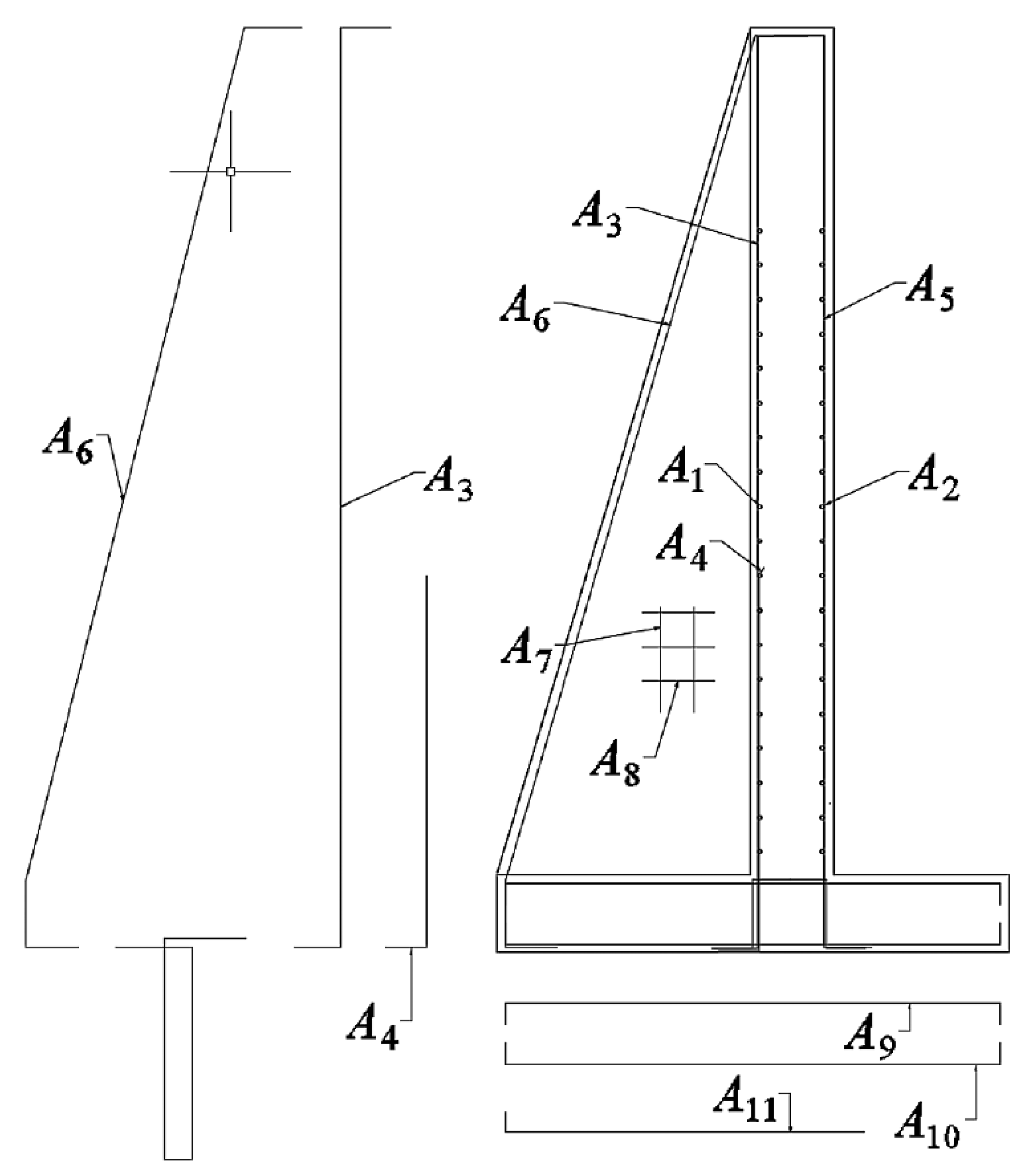
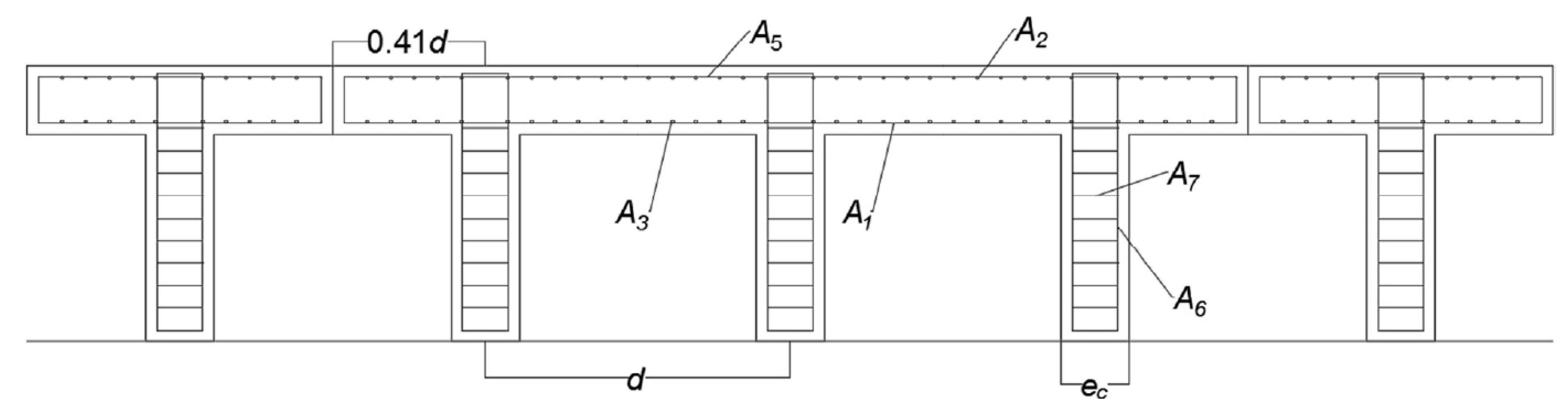
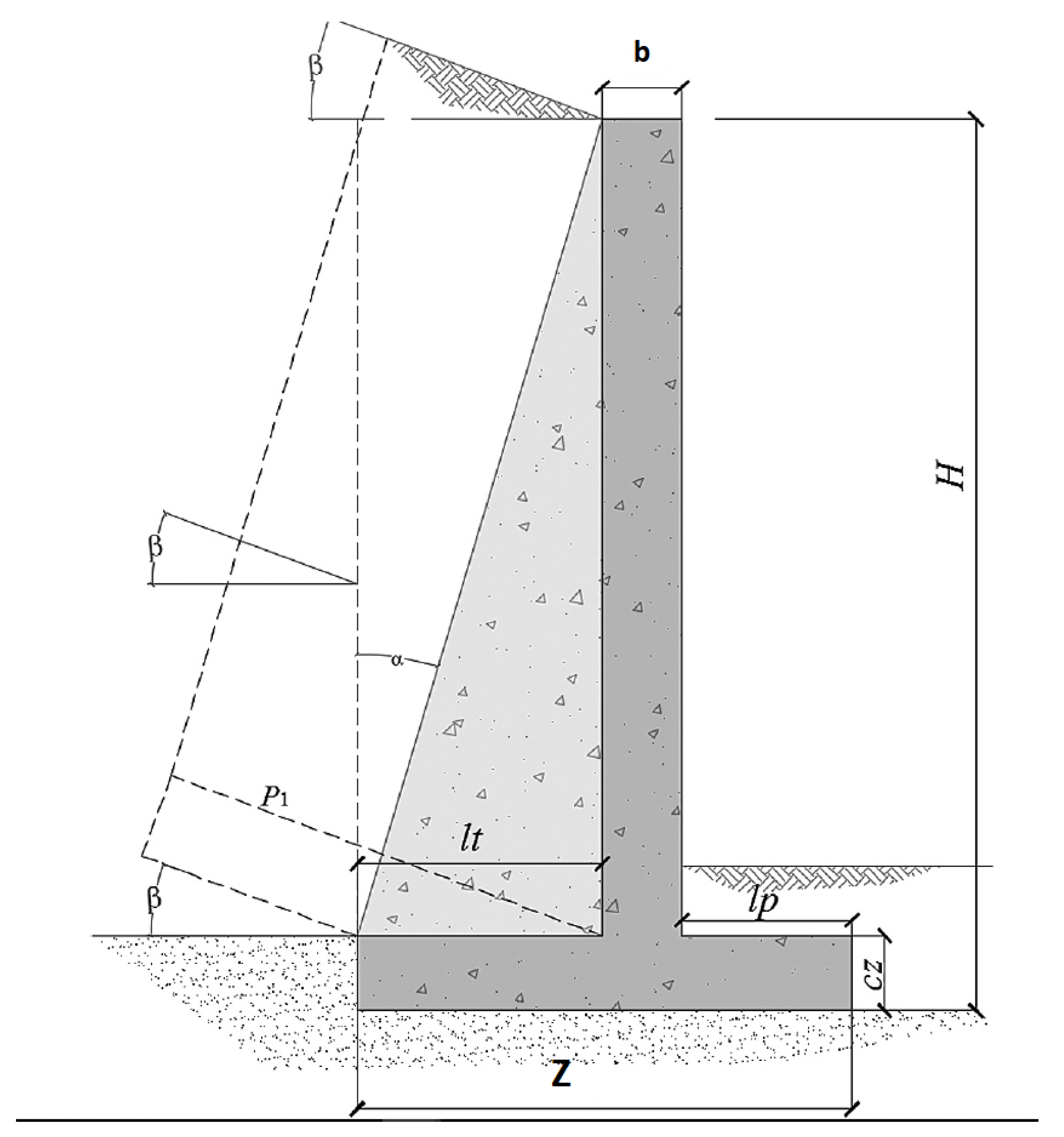
Of the set of variables, 24 are shown in Figure 2, Figure 3 and Figure 4. Figure 2 and Figure 3 represent the configuration of the reinforcement (A1–12), with the diameter and number of steel bars. Three flexural reinforcing bars defined as A1, A2 and A3 contribute to the main bending of the stem. A4 represents the vertical reinforcement of the base at the rear of the stem. The secondary longitudinal reinforcement is provided by A5 for shrinkage and thermal effects on the stem. A6 represents the longitudinal reinforcement of the buttress. The area of the reinforcing bracket from the bottom of the buttress is provided by A7 and A8. A9 and A11 define the upper and lower heel reinforcements and A12, the shear reinforcement in the footing. Finally, the longitudinal effects on the toe are defined by A10. Figure 4 represents most of the geometric variables.These variables are the thickness of the stem (b), the thickness of the footing (cz), the thickness of the buttresses (ec), the length of the heel (lt), the length of the toe (lp), the distance between the buttresses (d), two classes of steel B500S and B400S, and six classes of concrete between C25/30 and C50/60 by discrete intervals of 5 MPa.

Table 2. Design variables.

Variables	Lower Bound	Upper Bound	Increment
c	H/20	H/6	1 cm
d	H/4	H/2	1 cm
b	20 cm	219	1 cm
p	20 cm	610	1 cm
t	20 cm	619	1 cm
$e_c$	20 cm	219	1 cm
$f_{ck}$			25, 30, 35, 40, 45, 50 Mpa
$f_{yk}$			400, 500 Mpa
$A_1$ to $A_{10}$ $\mathsf{\Phi }$			6, 8, 10, 12, 16, 20, 25, 32 mm
n	1	12	1 rebar
$A_{11}$ to $A_{12}$ $\mathsf{\Phi }$			6, 8, 10, 12, 16, 20, 25, 32 mm
n	4	10	1 rebar

details the set of discrete variables with the ranges of the values they can take. The possible combinations constitute the space solutions of the problem. For the case of a 12 m high wall, the solution space is of the order of ${10}^{20}$.

3.3. Problem Design Parameters

All the cases analyzed in this study are completely defined by constant contour values called problem parameters. These parameters are described in [58] and are represented in

Table 3. Problem design parameters values.

Parameter Type	Parameter Considered	Value
Geometric:
	Foundation depth, H2	2 m
Geotechnical and relative to the load:
	Bearing capacity	0.3 MPa
	Fill slope	0
	Base-friction coefficient, $\mu$	tg ${30}^{\circ }$
	Wall-fill friction angle, $\delta$	$0^{\circ }$
	Uniform load on top of the fill, $\gamma$	10 kN/m${}^2$
Safety coefficient:
	Against sliding, ${\gamma }_{fs}$	1.5
	Against overturning, ${\gamma }_{fo}$	1.8
	For loading (EHE)	Normal
	Of concrete (ULS)	1.5
	Of steel (ULS)	1.15
Ambient exposure (EHE)		IIa

.

3.4. Problem Constrains

The viability of the structure is verified as described in [58], in accordance with the Spanish technical standards defined in [59] and the detailed recommendations for foundations in road works [60]. The bending and shear limit states, and the cracking limit state are verified. The structure is checked according to the stem stress distribution [61] for non-cohesive granular materials. The rectangular distribution of soil stresses in the foundations is considered according to the criteria in [62]. The structural hyperstatic model assumes that the top of the stem functions as a cantilever, while the bottom of the stem is embedded between the footing and the lower part of the buttress.

The bending stress verified in the horizontal T-shaped cross section is performed taking into account the effective width, in accordance with [63]. The checking of the mechanical shear and the flexural capacity is carried out considering the equations expressed in [62] and with the verifications in [59]. To assess the controls against overturning and sliding, and the limit of soil stresses, the effect of buttresses is included [58]. It is taken into account that the favorable overturning moments are sufficiently greater than the unfavorable overturning moments with a safety coefficient for frequent events. A slip safety coefficient and a coefficient of base-friction foundation against sliding are also considered.

4. The db-Scan Discrete Algorithm

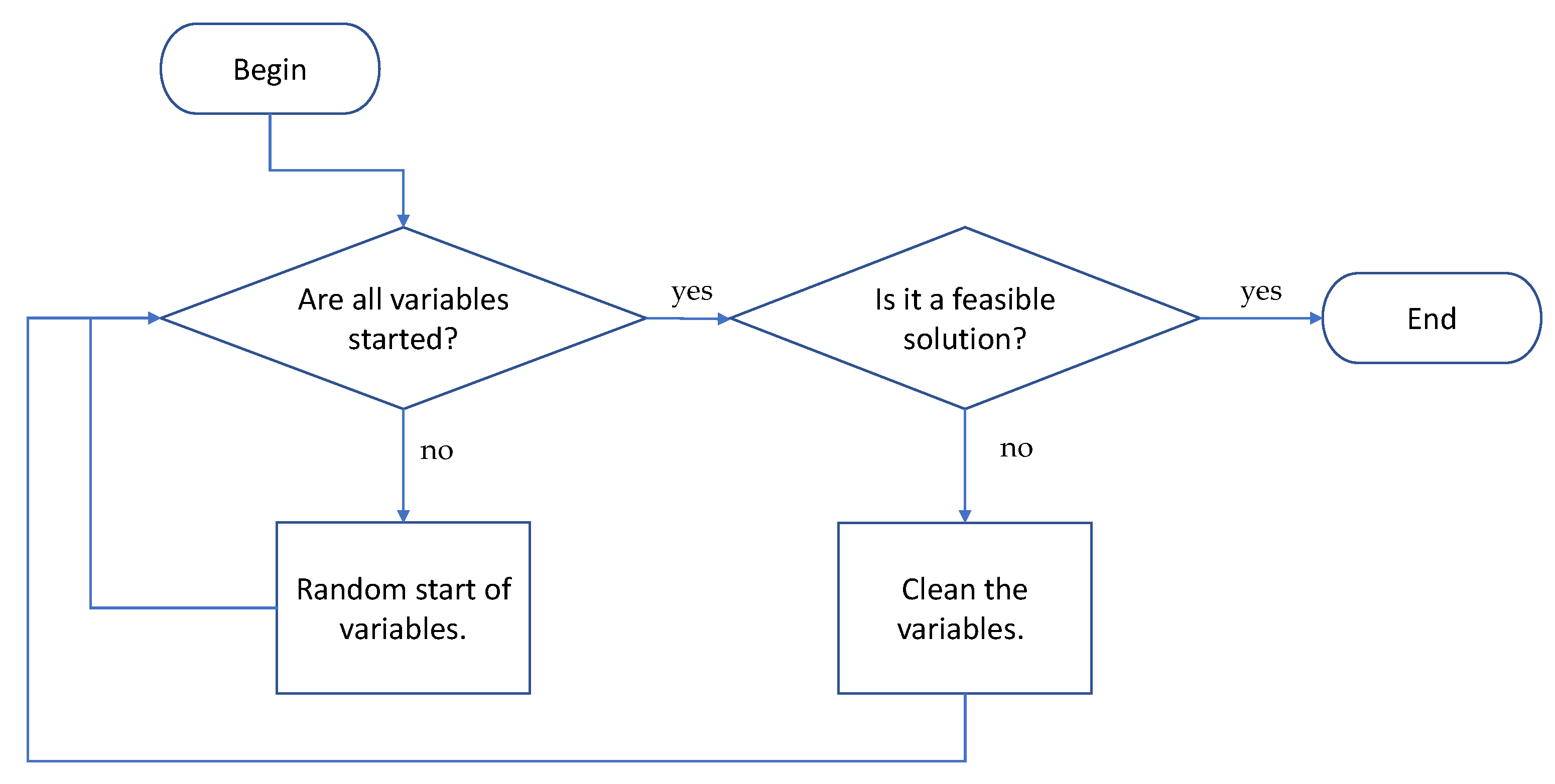
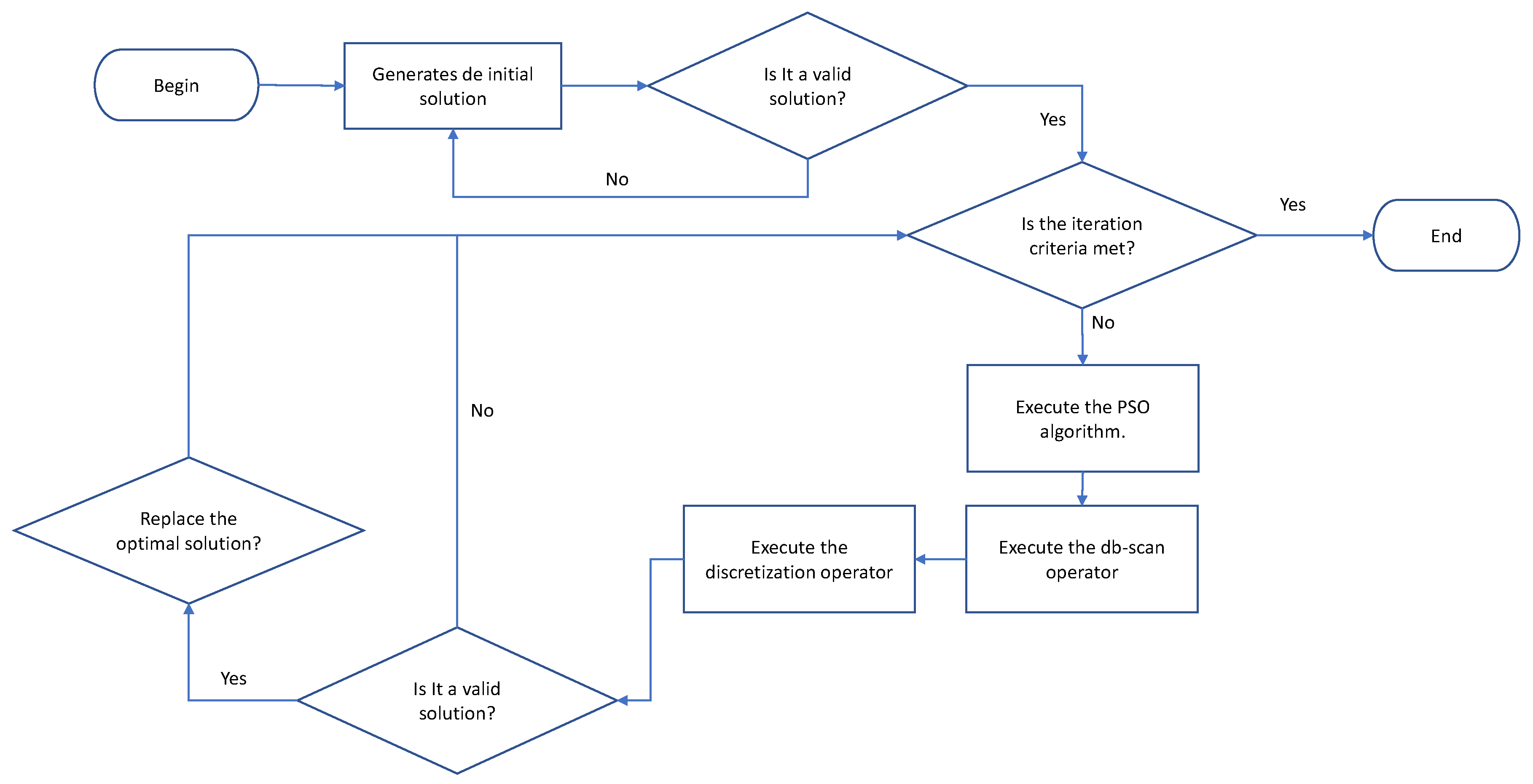
As a first step, the algorithm generates a set of valid solutions. These solutions are randomly generated. In this procedure, first, it is validated if the solution variables are started. In the case that they are not all started, the variables are started randomly. Once all the variables are generated, the next step is to verify if the solution obtained is valid. In the event that it is not valid, all variables are removed and regenerated. The detail of the initiation procedure is shown in Figure 5. Subsequently, PSO is used to produce a new solution in the continuous space. The PSO algorithm will be described in Section 4.1. Subsequently, the db-scan operator is applied to the continuous solution in order to transform continuous movements into groups associates to transition probabilities. The db-scan operator will be detailed in Section 4.2. After the db-scan operator generates the groups, the discretization operator applies the corresponding transition probability to each group, generating a new discrete solution. The discretization operator is detailed in Section 4.3. Finally, the new solution is validated and, in case it meets the restrictions, it is compared with the best solution obtained. If the new value is higher, it replaces the current one. The detailed flow chart of the hybrid algorithm is shown in Figure 6.

4.1. Particle Swarm Optimization

For the proper functioning of the PSO algorithm, the concepts of population that are usually called a swarm, and each of these solutions is called a particle. The essence of the algorithm is that each particle is guided by a combination of the best value particle obtained so far in the search space (maximum global) together with the best result obtained by the particle (local maximum). The optimization process is iterative until some termination condition is met.

Formally let $f:{\mathbb{R}}^n\to \mathbb{R}$ corresponds to the fitness function to be optimized. This function considers a candidate solution that is represented by a vector in ${\mathbb{R}}^n$ and generates a real value as output. This obtained value, represents the value of the objective function for the given candidate solution. The goal is to find a solution for which $f\left(a\right)\le f\left(b\right)$ for all b in the search space, which would mean that a is the global minimum. The algorithm pseudo-code is shown in Procedure 1.

Algorithm 1 Particle swarm optimization algorithm

1: Objective function f(s)  2: Generate initial solutions of n particles.  3: Get the particle’s best known position to its initial position: $p_i\leftarrow s_i$.  4: if$f\left(p_i\right)<f\left(g\right)$then  5:     Update the swarm’s best known position: $g\leftarrow p_i$  6: end if  7: Initialize the particle’s velocity: $v_i$  8: while stop criterion are meet do  9:     for each particle and dimension do 10:         Pick random numbers: $r_p,r_g$ 11:         Update the particle’s velocity: $v_{i,d}\leftarrow \omega v_{i,d}+{\varphi }_p{r}_p(p_{i,d}-s_{i,d})+{\varphi }_g{r}_g(g_d-s_{i,d})$ 12:         Update the particle’s position: $s_i\leftarrow s_i+v_i$ 13:     end for 14:     if $f\left(s_i\right)$ < $f\left(p_i\right)$ then 15:         Update the particle’s best known position: $p_i\leftarrow s_i$. 16:         if $f\left(p_i\right)$ < $f\left(g\right)$ then 17:             Update the swarm’s best known position: $p_i\leftarrow s_i$. 18:         end if 19:     end if 20: end while

4.2. db-Scan Operator

The solutions resulting from the execution of the PSO algorithm are grouped by the db-scan operator. We should note that the db-scan operator can be applied to any swarm intelligence continuous metaheuristics. The spatial clustering technique based on noise density of applications (db-scan), requires for the clustering, a set of points S within a vector space, and a metric, usually, the metric is the Euclidean. Db-scan groups the points of S that meet a minimum density criterion. The rest of the points are considered outliers. As input parameters db-scan requires a radius $ϵ$ and the minimum number of neighbors $\delta$. The main steps of the algorithm are shown below:

• Find the points in the $ϵ$ neighborhood of every point and identify the core points with more than $\delta$ neighbors.
• Find the connected components of core points on the neighbor graph, ignoring all non-core points.
• Assign each non-core point to a nearby cluster if the cluster is an $ϵ$ neighbor; otherwise, assign it to noise.

In the db-scan (dbscanOp) operator, the db-scan grouping technique is used to make groups of points to which we will assign a probability of transition. This probability of transition will subsequently allow the discretization operator to discretize continuous solutions. The grouping proposal uses the movements obtained by PSO in each dimension for all the particles. Suppose $s\left(t\right)$ is a solution in iteration t, then ${\Delta }^i\left(s\left(t\right)\right)$ represents the magnitude of the offset $\Delta \left(s\right(t\left)\right)$ in the i-th position, considering the iterations t and $t+1$. After all the displacements were obtained, the grouping is carried out. To obtain the groups, the displacement module will be used, which is denoted by $|{\Delta }^i\left(s\left(t\right)\right)|$. This grouping is done using the db-scan technique. Finally, a generic function $P_{tr}$ is used, which is shown in Equation (2) with the objective of assigning a probability of transition to each group and therefore to each displacement.

Then using the function $P_{tr}$, a probability is assigned to each group obtained from the clustering process. In this article, we use the linear function given in Equation (2), where Clust ($x^i$) indicates the location of the group to which ${\Delta }^i\left(s\right)$ belongs. The coefficient $\alpha$ represents the initial transition coefficient and $\beta$ models the transition separation for the different groups. Both parameters must be estimated. The pseudo-code of the discretization procedure is shown in Algorithm 2.

$$P_{tr}\left(x\right)=\alpha +\gamma x$$

(2)

where x represents the value of $Clust\left(s^i\right)$. Also, because $s^i\in Clust\left(s^i\right)$, each element of $Clust\left(s^i\right)$, is assigned the same value $P_{tr}$. That is, $P_{tr}\left(s^i\right)=P_{tr}\left(Clust\left(s^i\right)\right)$. On the other hand, $\gamma =\alpha \ast \beta$ are constants that will be determined in the tuning of parameters, where $\alpha$ corresponds to the initial transition coefficient and $\beta$ represents the transition probability coefficient.

Algorithm 2 db-scan operator

1: Function dbscanOp($ls\left(t\right)$,$ls(t+1)$) 2: Input$s\left(t\right)$, $s(t+1)$ 3: Output lTransitionProbability$(t+1)$ 4: $l{\Delta }^i\left(s(t+1)\right)\leftarrow$ getDelta($ls\left(t\right)$, $ls(t+1)$) 5: $Clust\leftarrow$ getClusters($l{\Delta }^i\left(s\left(t\right)\right)$) 6: lTransitionProbability$(t+1)$← getTranProb($Clust$, $ls\left(t\right)$)–Equation (2) 7: return (lTransitionProbability$(t+1)$)

4.3. Discretization Operator

The discretization operator receives the list lTransitionProbability $(t+1)$. This list contains the values of the transition probabilities which were the result delivered by the db-scan operator. Then given a solution $s\left(t\right)\in ls\left(t\right)$, we select each of its components $s^i\left(t\right)$ and we proceed to determine through the transition probability if this component should be modified. In the case of large transition probabilities, there is a greater possibility of modification. Then a random number is obtained at [0, 1] and this number is compared with the value of the transition probability assigned to the component. In cases where the modification condition is satisfied, it can increase the value by 1 or decrease it by 1. Finally, the selected value is compared with the best value obtained by the algorithm and remains with the minimum of both. The pseudocode of the discrete procedure is shown in Algorithm 3.

Algorithm 3 Discretization operator.

1: Function DiscOperator(lTransitionProbability$(t+1)$, $ls\left(t\right)$)  2: Input lTransitionProbability$(t+1)$  3: Output$s(t+1)$–where $s(t+1)$ is discrete.  4: movement = 0  5: for$s^i\in s\left(t\right)\in ls\left(t\right)$do  6:     if $r_1>0.5$then  7:         movement = 1  8:     else  9:         movement = −1 10:     end if 11:     $s^i$ = max(1,min($s_{best}^i$,$s^i$+movement)) 12: end for

5. Results and Discussion

The experiments developed with the objective of determining the performance of our hybrid algorithm applied to the counterfort retaining wall problem will be detailed in this section. In Section 5.1, we will explain the strategy used to perform the tuning of the parameters. Then, in the first experiment detailed in Section 5.2, we will study the contribution of the db-scan operator to the discretization process. This study will be carried out through a comparison with a random operator. Subsequently, in the second experiment, the db-scan technique will be compared with the k-means clustering technique. This comparison is detailed in Section 5.3. Finally, in Section 5.4 our db-scan PSO proposal will be compared with another algorithm in the literature that solved the same problem. Regarding the scenario of the experiments, each problem will be run 30 times. The value 30 is the minimum number appropriate to be able to obtain statistical conclusions on a population [64], in addition, the signed-rank Wilcoxon test [65] will be incorporated to determine if the difference between the results is statistically significant. For this test, the p-value used was $0.05$. The software was built in Python 3.6 and run on a computer with the following configuration: Intel Core i7-4770 CPU and 16 GB of RAM.

5.1. Parameter Settings

In the methodology used to perform the adjustment of the algorithm parameters, heights of 8 and 12 m were considered. The selection of these heights was motivated by their difference in complexity. 8 represents walls of small size and 12 represents walls of a greater size where the satisfaction of stability restrictions has a greater difficulty. After defining the instances to use, each of the defined configurations was resolved 5 times for each height. The set of configurations used are detailed in

Table 4. Parameter setting for the PSO algorithm.

Parameters	Description	Value	Range
$\alpha$	Initial transition coefficient	0.1	[0.08, 0.1, 0.12]
$\beta$	Transition probability coefficient	0.4	[0.3, 0.4, 0.5]
N	Number of particles	20	[10, 20, 30]
$ϵ$	$ϵ$ db-scan parameter	0.25	[0.2, 0.25, 0.3]
$minPts$	Point db-scan parameter	10%	[10, 12, 14]
Iteration Number	Maximum iterations	900	[800, 900, 1000]

. The value 5 was chosen with the intention of being able to execute all the combinations in a limited time. The range column in Table 4 represents the scanned values to perform the PSO adjustment. Obtaining these ranges was based on previous studies where the db-scan technique was applied to other combinatorial problems. For more details on the method, see the reference [26].

In order to find the best configuration, the method proposes using four measurements. The best solution (bs), the worst solution (ws), the average solution (as) and the convergence time (ct). These measures are defined in Equations (3)–(6). The best global value (bgv) corresponds to the best value obtained in all the configurations executed. Furthermore, the best local value (blv) represents the best value obtained by a particular configuration. The worst local value (wlv) represents the worst moment obtained for a given configuration. The average local value (alv) is the average value obtained by a configuration. The minimum global time (mgt) accounts for the minimum convergence time resulting from all evaluated configurations and the convergence local time (clt) the minimum time for a particular configuration. The minimum global time (mgt) corresponds to the best value getting for all configuration. Finally, the worst global value (wgv) accounts for the worst value obtained by all the configurations. Each of the measures defined, the closer to 1, the better performance that indicator has. On the other hand, the closer to 0, the worse performance. Since there are 4 measurements to be able to carry out the evaluation, we incorporate them into a radar graph and calculate their area. As a consequence of the measurement definition, the largest area corresponds to the configuration that has the best performance considering the 4 defined measurements.

Definition 1 

([10,26]). Measure definitions:

1. 

The deviation of the best local value obtained in five executions compared with the best global value:

$$bs=1-\frac{bgv-blv}{bgv}$$

(3)

2. 

The deviation of the worst value obtained in five executions compared with the best global value:

$$ws=1-\frac{bgv-wlv}{bgv}$$

(4)

3. 

The deviation of the average value obtained in five executions compared with the best global value:

$$as=1-\frac{bgv-alv}{bgv}$$

(5)

4. 

The convergence time for the average value in each experiment is normalized according to Equation (6).

$$ct=1-\frac{clt-mgt}{wgv-mgt}$$

(6)

For PSO, the coefficients $c_1$ and $c_2$ are set to 2. The parameter $\omega$ linearly decreases from 0.9 to 0.4. For the parameters used by db-scan, the minimum number of neighbors ($minPts$) is estimated as a percentage of the number of particles (N). The parameter settings are shown in Table 4. In the table, the column labeled “Value” represents the selected value, and the column labeled “Range” corresponds to the set of scanned values.

5.2. db-Scan and Random Operators Comparison

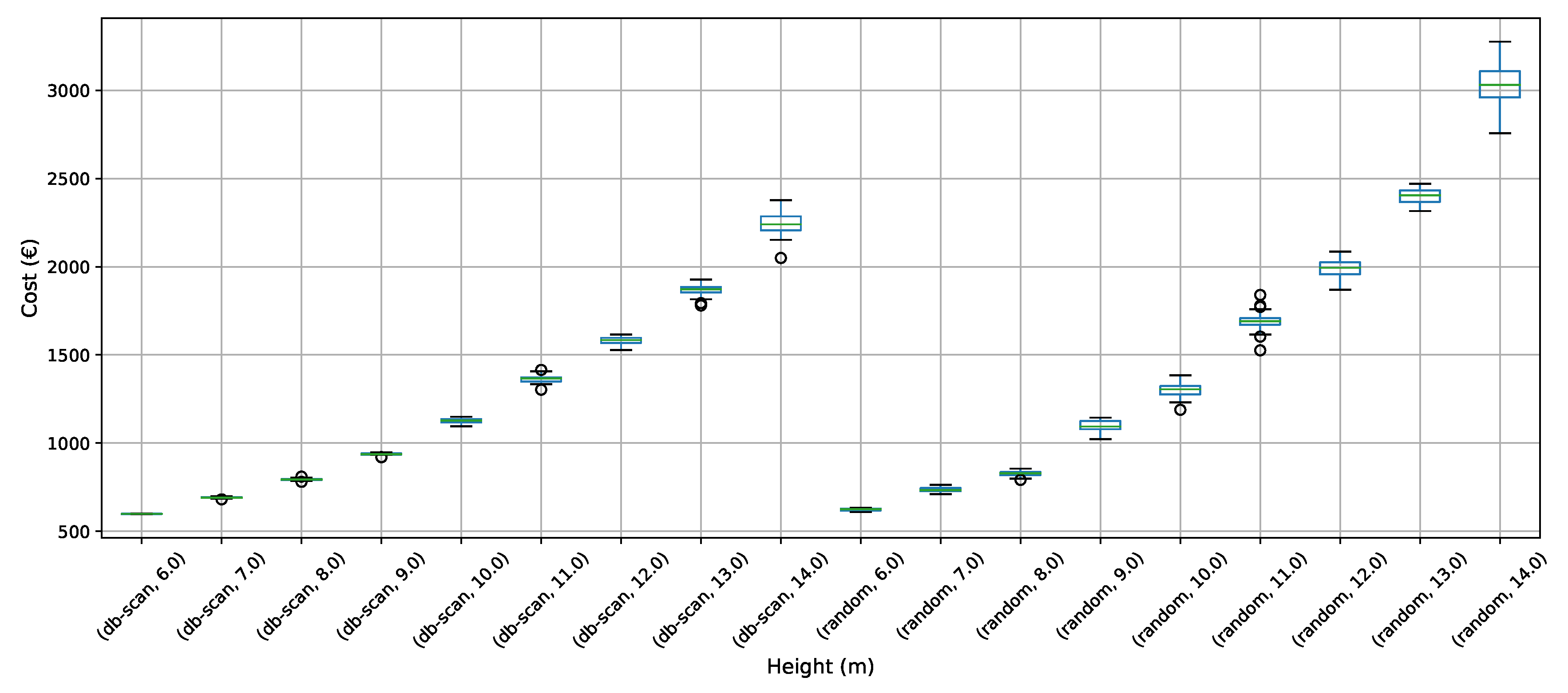
In this first experiment, the contribution of the db-scan operator in optimizing costs and emissions for the design of the wall will be studied. To properly determine the contribution of the db-scan operator, a random operator was designed to replace the discretization performed by db-scan. In particular, the execution of the db-scan operator in Figure 6 is replaced by a random operator. This random operator assigns a fixed probability of 0.5 instead of assigning probabilities per group. Different heights of the wall were considered, starting at 6 (m) and ending at 14 (m) with increments of one meter. For a proper statistical comparison, 30 runs are executed for each height and operator. The results are then documented in tables and boxplots. Finally, the Wilcoxon signed-rank test is used to determine the significance of the results.

Table 5. Comparison between random and db-scan operators in cost and emission optimization.

Height	Best Cost	Avg Cost	Best Emissions	Avg	Best Cost	Avg Cost	Best Emissions	Avg
(m)	Value	db-Scan	Value	Emissions	Value	Random	Value	Emissions
	db-Scan		db-Scan	db-Scan	Random		Random	Random
6	595	598.38	1249	1254.24	608	622.64	1287	1302.92
7	680	691.53	1452	1460.05	711	735.21	1470	1498.69
8	780	793.57	1662	1679.95	791	827.26	1717	1783.61
9	920	937.40	1997	2069.05	1022	1094.61	2190	2215.22
10	1095	1126.22	2462	2546.37	1188	1300.18	3050	3131.50
11	1302	1363.15	3061	3148.37	1526	1694.54	3614	3816.46
12	1528	1581.43	3715	3900.52	1870	1994.33	4299	4547.35
13	1780	1864.57	4470	4643.26	2315	2401.84	5180	5473.56
14	2049	2245.28	5294	5502.76	2756	3032.15	6048	6468.52
Wilcoxon						$4.31\times {10}^{-6}$		$1.87\times {10}^{-5}$
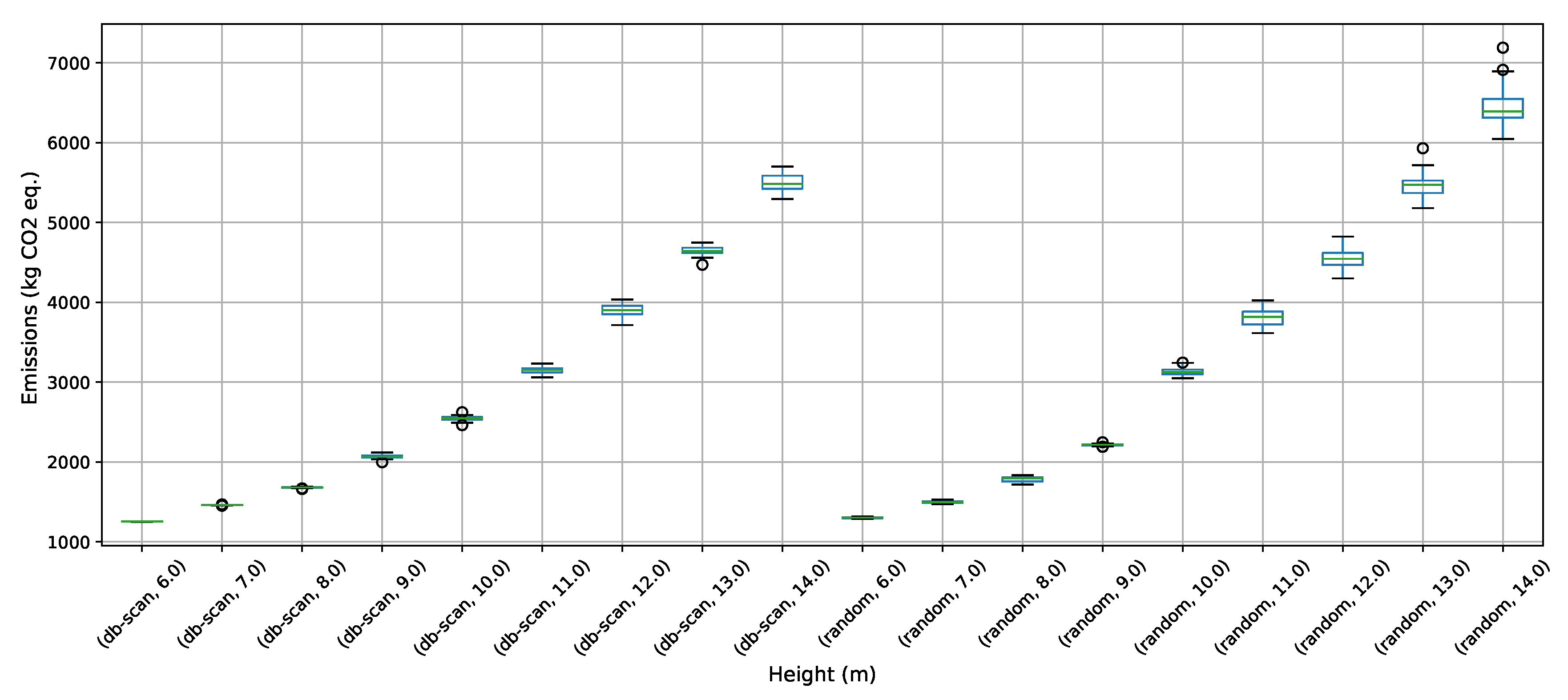
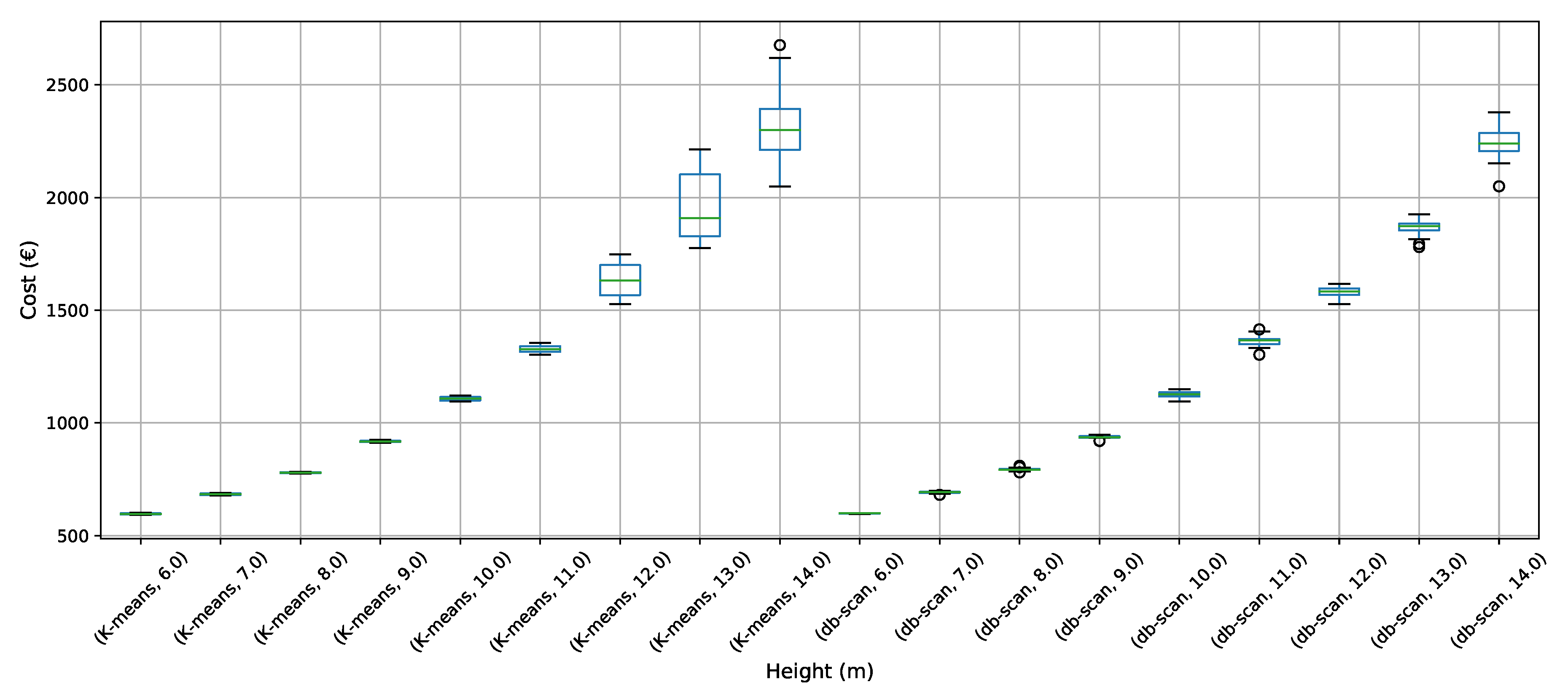
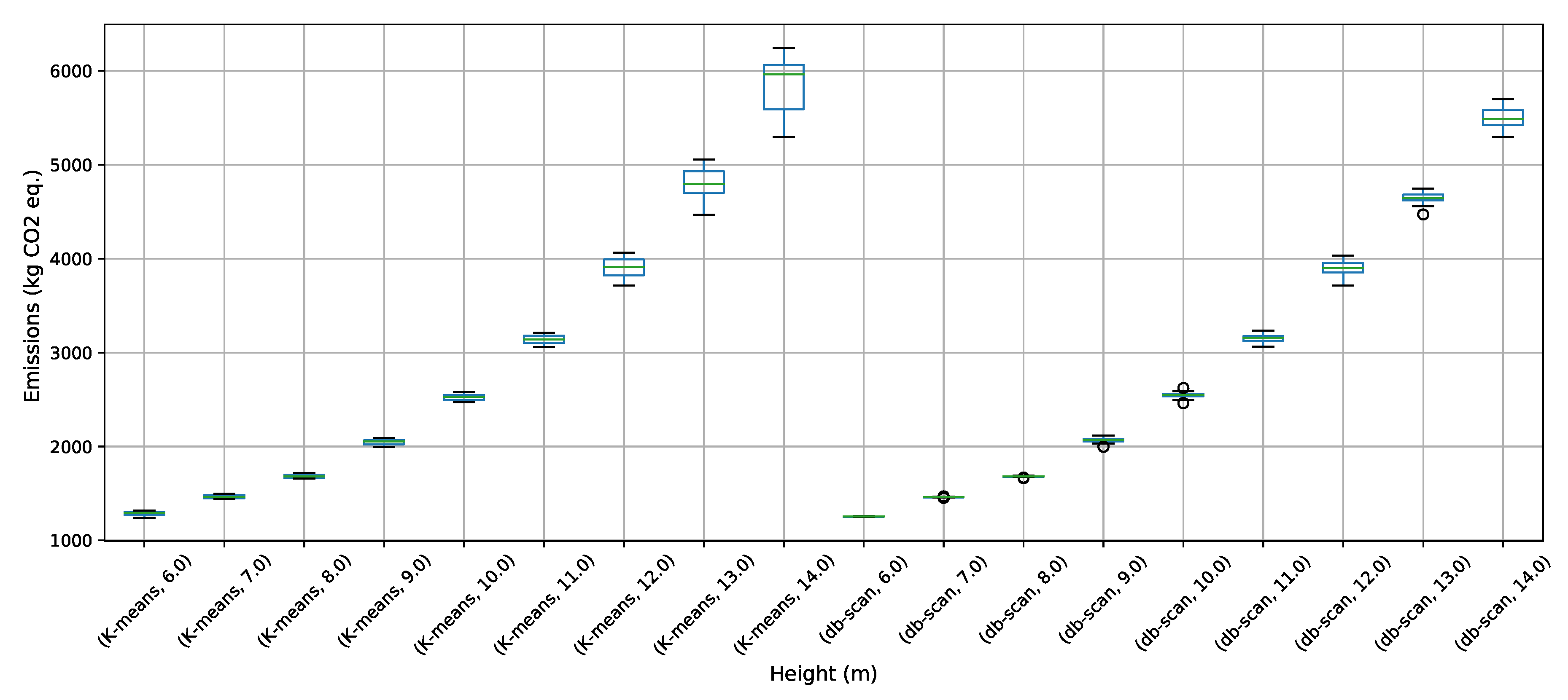
p-value

, Figure 7 and Figure 8 detail the results obtained in experiment 1. When comparing the values in Figure 7, in the case of the best value indicator, the operator that uses db-scan was Superior at all heights for both cost and emissions. Additionally, we observe the difference between the operators increases as the height increases. In the case of 6 and 7 m in the case of cost, the difference is 2.2% and 4.6% respectively. In the case of heights of 13 and 14 m, this difference is 30.0% and 34.5% respectively. When carrying out this same analysis for the emissions of CO${}_2$, we find that for the heights of 6 and 7 the differences are 3.0% and 1.2% respectively and at the heights of 13 and 14 we obtain 15.9% and 14.2% respectively. In the comparison of the average indicator, we see a very similar result to that reported in the best value analysis. The average indicator of the db-scan operator is higher for all heights than the random operator in both optimizations. Like the best value case, the difference increases as the height increases. In the case of averages, because the number of values is greater than in the case of the best value, we apply the Wilcoxon significance test. The result indicates that the difference is statistically significant in both cases, costs, and emissions. In Figure 7 we show the boxplots for the cost optimization results. In both cases, db-scan and random it is observed that the dispersion and the Inter-quartile range of the values obtained in the optimization increases as the height increases. However, from height 9 onwards this dispersion is more noticeable in the case of the random operator. When analyzing the results of the optimization of CO${}_2$, emissions, which are shown in Figure 8, the behavior is very similar to that of cost. In the case of emissions, the increase in dispersion and in the inter-quartile range is more noticeable in the random operator from the height of 11 m.

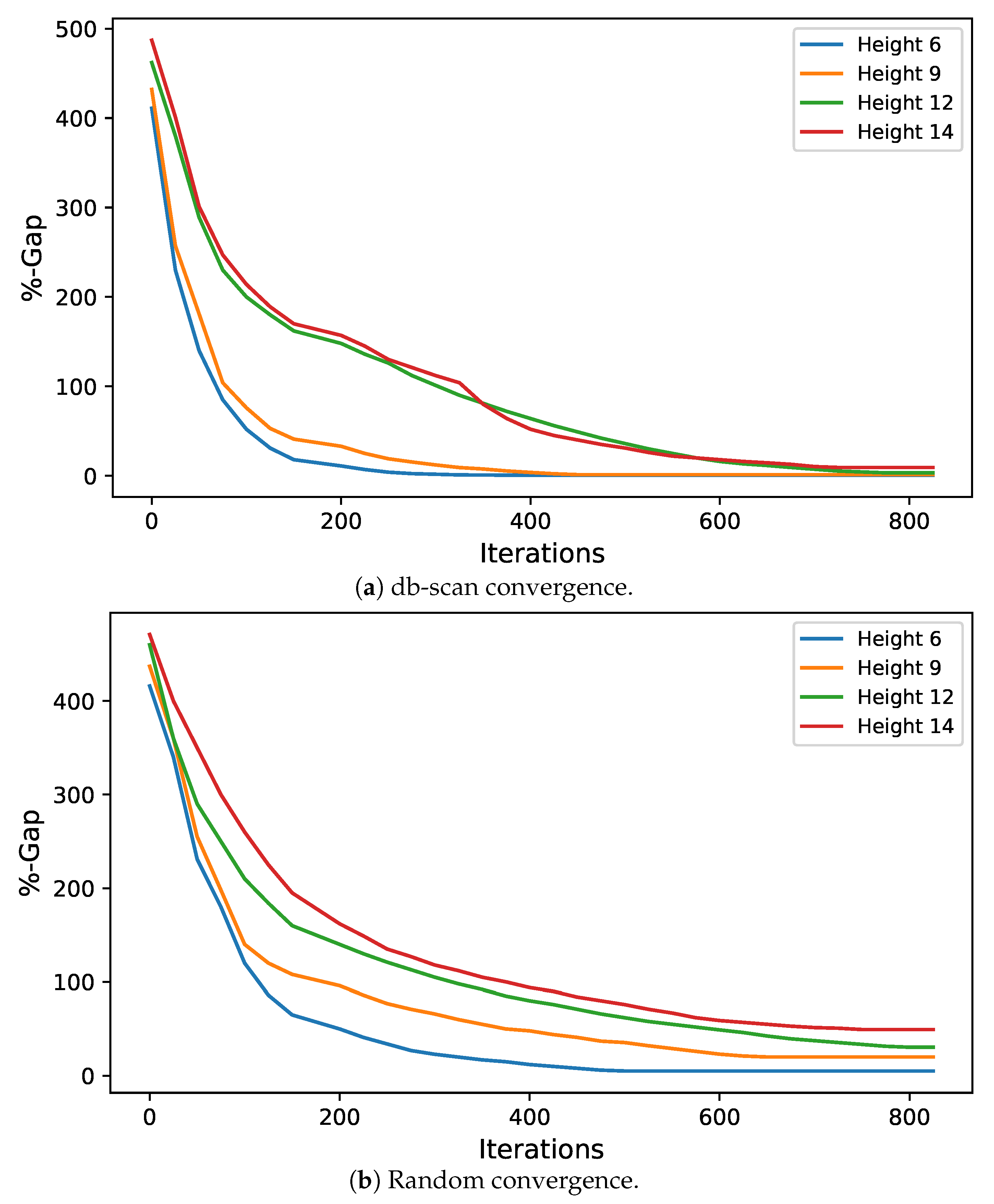
The convergence diagrams for heights 6, 9, 12 and 14 are shown in Figure 9a,b. These diagrams correspond to the results obtained in cost optimization using the random and db-scan operators. From the db-scan convergence chart, we see that height 6 has the best convergence, followed closely by 9. On the other hand, heights 12 and 14 have a similar convergence, being slower than the case of 6 and 9. At higher wall heights, complying with constraints becomes more complicated and therefore the optimization problem is more difficult to solve. In the case of the random operator, it shows a correspondence between the height and the speed of convergence. The lower the height, the better its convergence. On the other hand, we see that for the random case, already in the 500 iterations the slope tends to stabilize unlike in the db-scan case where for the most difficult problems the slope stabilizes after the 600 iterations.

5.3. db-Scan and k-Means Operators Comparison

This second experiment aims to compare the performance of the algorithm that uses db-scan, with another algorithm that uses k-means as a discretization method. This experiment is inspired by the fact that both techniques correspond to unsupervised learning algorithms that aim to cluster points. In the case of k-means, unlike db-scan, the number of clusters must be defined a priori. In this experiment, suggested by the articles [10,26], k was configured with the value 5. The Equation (2) was used to set the values of the probability of transition for each cluster. As in experiment 1, the db-scan module in Figure 6 is replaced in this case by k-means leaving the rest of the modules unchanged.

The results of this experiment are shown in

Table 6. Comparison between db-scan and k-means operators in cost and emission optimization.

Height	Best Cost	Avg Cost	Best Emissions	Avg	Best Cost	Avg Cost	Best Emissions	Avg
(m)	Value	db-Scan	Value	Emissions	Value	k-Means	Value	Emissions
	db-Scan		db-Scan	db-Scan	k-Means		k-Means	k-Means
6	595	598.38	1249	1254.24	591	596.35	1242	1284.92
7	680	691.53	1452	1460.05	678	683.62	1440	1465.52
8	780	793.57	1662	1679.95	775	779.34	1659	1685.83
9	920	937.40	1997	2069.05	911	938.24	1997	2046.26
10	1095	1126.22	2462	2546.37	1095	1107.80	2470	2523.35
11	1302	1363.15	3061	3148.37	1302	1327.16	3061	3139.20
12	1528	1581.43	3715	3900.52	1528	1638.84	3715	3902.61
13	1780	1864.57	4470	4643.26	1775	1958.62	4470	4798.79
14	2049	2245.28	5294	5502.76	2049	2322.87	5294	5821.08
Wilcoxon						0.42		$4.08\times {10}^{-4}$
p-value

and Figure 10 and Figure 11. When analyzing the results of the best value indicator shown in Table 6, we observed in the case of cost optimization, the results are similar, with k-means being higher in 5 of the 9 heights. In the case of optimization of CO${}_2$ emissions, something similar occurs, with very close values between the two algorithms. In the last case, k-means was higher in 3 cases, db-scan in 1, and in 4 heights their values coincided. When analyzing the average indicator, in the case of optimizing the cost of the wall, we observe that for small heights very close values are obtained in both algorithms, being k-means higher than db-scan. Particularly in the case of heights 6, 7, 8 the difference in percentage was 0.34%, 1.16%, and 1.83% respectively. On the other hand, when we analyze the values obtained in the highest walls, we find that db-scan is superior to k-means. Particularly for heights 12, 13, and 14, we have that the difference is 3.63%, 5.04%, and 3.46% respectively. Wilcoxon’s statistical test when analyzing the total population indicates that the difference between both algorithms is not significant. In the case of emission optimization, the behavior of the average indicator is different from that of cost optimization. The db-scan algorithm is superior in 6 of the 9 heights in this indicator. Heights 13 and 14 stand out, achieving differences of 3.3% and 5.78% respectively. When analyzing the total distribution of points, the Wilcoxon test indicates that the difference is significant in favor of db-scan.Finally, when analyzing Figure 10 and Figure 11 both algorithms have a similar behavior between heights 6 and 11. From height 12 onwards, the increase in dispersion and in the Inter-quartile range becomes much more notorious in the case of k-means. This last result shows that for more difficult problems, db-scan behaves more robust than k-means.

5.4. db-Scan PSO and HS Comparison

The third experiment aims to compare the hybrid db-scan PSO algorithm with results published in the literature. We particularly consider the results published in [18,58]. In these articles, a variant of the HS algorithm for the optimization of buttress retaining walls was developed. To carry out the evaluation, the same procedure as the previous experiments will be followed, i.e., through the best value and average indicators supplemented with boxplots and the Wilcoxon test for the statistical significance of the results.

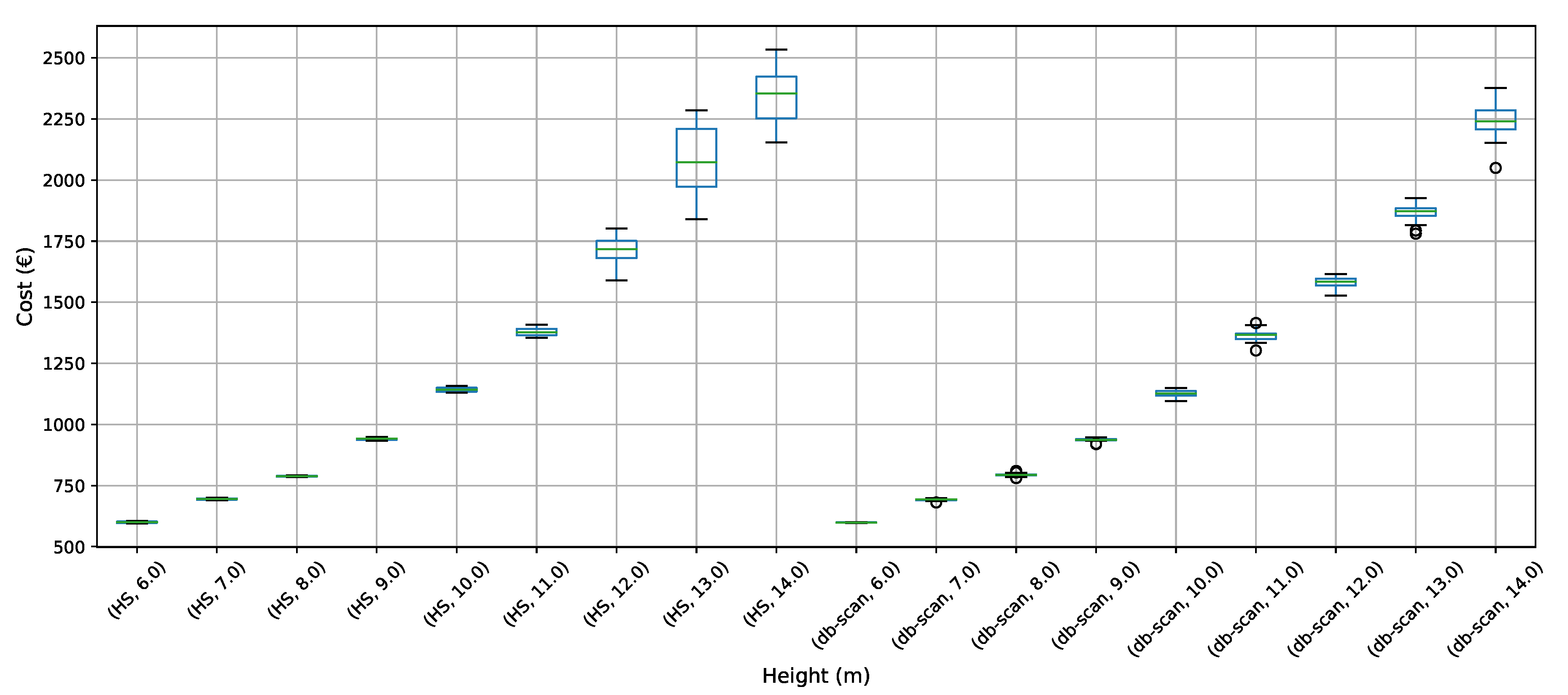
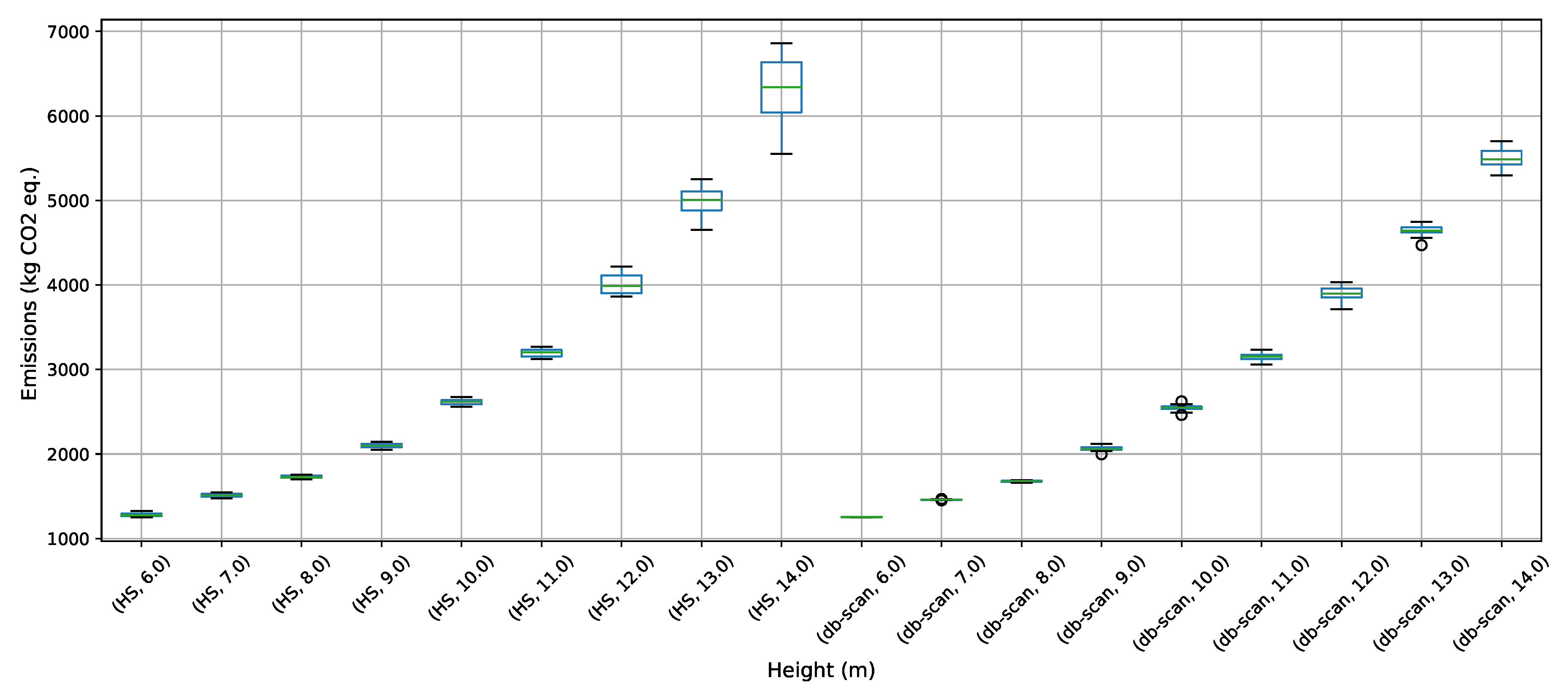
The comparison of both algorithms is documented in

Table 7. Comparison between db-scan PSO and HS algorithms in cost and emission optimization.

Height	Best Cost	Avg Cost	Best Emissions	Avg	Best Cost	Avg Cost	Best Emissions	Avg
(m)	Value	db-Scan	Value	Emissions	Value	HS	Value	Emissions
	db-Scan		db-Scan	db-Scan	HS		HS	HS
6	595	598.38	1249	1254.24	595	600.15	1250	1289.14
7	680	691.53	1452	1460.05	689	694.98	1478	1511.53
8	780	793.57	1662	1679.95	784	788.38	1699	1731.54
9	920	937.40	1997	2069.05	934	941.29	2050	2097.45
10	1095	1126.22	2462	2546.37	1130	1143.64	2560	2617.81
11	1302	1363.15	3061	3148.37	1354	1381.50	3124	3201.45
12	1528	1581.43	3715	3900.52	1590	1707.24	3865	4046.95
13	1780	1864.57	4470	4643.26	1840	2067.37	4650	4955.95
14	2049	2245.28	5294	5502.76	2154	2348.71	5550	6241.00
Wilcoxon						$4.17\times {10}^{-7}$		$2.24\times {10}^{-8}$
p-value

and in Figure 12 and Figure 13. When analyzing the best value indicator, the db-scan PSO algorithm is superior in 8 of the 9 instances to HS. In optimizing emissions of CO${}_2$, in 9 of the 9 instances, db-scan performs better. When evaluating the average indicator, the situation is similar to reported by the best value indicator. In 8 of 9 heights of the wall, db-scan PSO has better performance for cost optimization and in the 9 heights, it is superior for emissions. Wilcoxon’s test indicates that in both cases the difference is significant. When analyzing the Figure 12 and Figure 13 we observe that from height 12 onwards, the dispersion and the inter-quartile range of HS solutions grow significantly concerning db-scan PSO.

6. Conclusions

To address the buttressed walls problem, a hybrid algorithm based on the db-scan clustering technique and the PSO optimization algorithm was proposed in this article. This hybridization was necessary because PSO works naturally in continuous spaces and the problem studied is combinatorial. A Db-scan was used as a discretization mechanism. The optimization functions considered were cost and emission of CO${}_2$. To measure the robustness of our proposal, three experiments were designed. The first evaluates the performance of the hybrid algorithm with respect to a random operator. Later in the second experiment, the performance was compared with respect to the k-means clustering technique. Finally, in the last experiment, we studied the performance of the hybrid algorithm when compared to an HS adaptation described in the literature. The first experiment concludes that the db-scan operator contributes to the quality of the solutions, obtaining better values than the random operator, in addition to reducing the dispersion of these. In comparison with k-means mixed results are obtained, in some cases, k-means is superior to db-scan and in other db-scan improves the solutions obtained by k-means. Regarding the dispersion in the different instances, we observed that from height 12 onwards db-scan obtained much smaller dispersions than k-means. Lastly, in comparison with HS, in general, db-scan surpass HS obtaining better results, especially in the instances where the height was over 12 m.

From the results obtained in this study, several lines of research emerge. The first line is related to population management. In the present work, the population was a static parameter. By analyzing the results generated by the algorithm as it iterates, it is possible to identify regions where search needs to be intensified or regions where further exploration is needed. This would allow for dynamic population management. Another interesting research line is related to the parameters used by the algorithm. According to what is detailed in Section 5.1, a robust method was used to get the most suitable configuration. However, this configuration is a static one and is not necessarily the best configuration throughout all execution. Proposing a framework that allows adapting the parameters based on the results obtained by the algorithm as it is executed, would allow generating even more robust methods than the current one.

References

- Carbonell, A.; González-Vidosa, F.; Yepes, V. Design of reinforced concrete road vaults by heuristic optimization. Adv. Eng. Softw. 2011, 42, 151–159. [Google Scholar]
- Yepes, V.; Alcala, J.; Perea, C.; González-Vidosa, F. A parametric study of optimum earth-retaining walls by simulated annealing. Eng. Struct. 2008, 30, 821–830. [Google Scholar] [CrossRef]
- García, J.; Lalla-Ruiz, E.; Voß, S.; Droguett, E.L. Enhancing a machine learning binarization framework by perturbation operators: Analysis on the multidimensional knapsack problem. Int. J. Mach. Learn. Cybern. 2020. [Google Scholar] [CrossRef]
- García, J.; Moraga, P.; Valenzuela, M.; Pinto, H. A db-Scan Hybrid Algorithm: An Application to the Multidimensional Knapsack Problem. Mathematics 2020, 8, 507. [Google Scholar] [CrossRef] [Green Version]
- García, J.; Crawford, B.; Soto, R.; Astorga, G. A clustering algorithm applied to the binarization of Swarm intelligence continuous metaheuristics. Swarm Evol. Comput. 2019, 44, 646–664. [Google Scholar]
- García, J.; Moraga, P.; Valenzuela, M.; Crawford, B.; Soto, R.; Pinto, H.; Pe na, A.; Altimiras, F.; Astorga, G. A Db-Scan Binarization Algorithm Applied to Matrix Covering Problems. Comput. Intell. Neurosci. 2019, 2019. [Google Scholar] [CrossRef] [Green Version]
- Saeheaw, T.; Charoenchai, N. A comparative study among different parallel hybrid artificial intelligent approaches to solve the capacitated vehicle routing problem. Int. J. Bio-Inspir. Comput. 2018, 11, 171–191. [Google Scholar] [CrossRef]
- Crawford, B.; Soto, R.; Astorga, G.; García, J. Constructive metaheuristics for the set covering problem. In International Conference on Bioinspired Methods and Their Applications; Springer: Berlin, Germany, 2018; pp. 88–99. [Google Scholar]
- García, J.; Altimiras, F.; Pe na, A.; Astorga, G.; Peredo, O. A binary cuckoo search big data algorithm applied to large-scale crew scheduling problems. Complexity 2018, 2018. [Google Scholar] [CrossRef]
- García, J.; Martí, J.; Yepes, V. A Hybrid k-Means Cuckoo Search Algorithm Applied to the Counterfort Retaining Walls Problem. Mathematics 2020, 8, 555. [Google Scholar] [CrossRef]
- Marti-Vargas, J.R.; Ferri, F.J.; Yepes, V. Prediction of the transfer length of prestressing strands with neural networks. Comput. Concr. 2013, 12, 187–209. [Google Scholar] [CrossRef]
- Penadés-Plà, V.; García-Segura, T.; Yepes, V. Robust Design Optimization for Low-Cost Concrete Box-Girder Bridge. Mathematics 2020, 8, 398. [Google Scholar]
- García-Segura, T.; Yepes, V.; Frangopol, D.M.; Yang, D.Y. Lifetime reliability-based optimization of post-tensioned box-girder bridges. Eng. Struct. 2017, 145, 381–391. [Google Scholar] [CrossRef]
- Sierra, L.A.; Yepes, V.; García-Segura, T.; Pellicer, E. Bayesian network method for decision-making about the social sustainability of infrastructure projects. J. Clean. Prod. 2018, 176, 521–534. [Google Scholar]
- Yepes, V.; Martí, J.V.; García-Segura, T. Cost and CO2 emission optimization of precast–prestressed concrete U-beam road bridges by a hybrid glowworm swarm algorithm. Autom. Constr. 2015, 49, 123–134. [Google Scholar] [CrossRef]
- Yepes, V.; Gonzalez-Vidosa, F.; Alcala, J.; Villalba, P. CO2-optimization design of reinforced concrete retaining walls based on a VNS-threshold acceptance strategy. J. Comput. Civ. Eng. 2012, 26, 378–386. [Google Scholar] [CrossRef] [Green Version]
- Yepes, V.; Martí, J.V.; García, J. Black Hole Algorithm for Sustainable Design of Counterfort Retaining Walls. Sustainability 2020, 12, 2767. [Google Scholar] [CrossRef] [Green Version]
- Molina-Moreno, F.; Martí, J.V.; Yepes, V. Carbon embodied optimization for buttressed earth-retaining walls: Implications for low-carbon conceptual designs. J. Clean. Prod. 2017, 164, 872–884. [Google Scholar] [CrossRef]
- Kaveh, A.; Biabani Hamedani, K.; Zaerreza, A. A set theoretical shuffled shepherd optimization algorithm for optimal design of cantilever retaining wall structures. Eng. Comput. 2020. [Google Scholar] [CrossRef]
- Mergos, P.E.; Mantoglou, F. Optimum design of reinforced concrete retaining walls with the flower pollination algorithm. Struct. Multidiscipl. Optim. 2020, 61, 575–585. [Google Scholar]
- Pons, J.J.; Penadés-Plà, V.; Yepes, V.; Martí, J.V. Life cycle assessment of earth-retaining walls: An environmental comparison. J. Clean. Prod. 2018, 192, 411–420. [Google Scholar] [CrossRef]
- Zastrow, P.; Molina-Moreno, F.; García-Segura, T.; Martí, J.V.; Yepes, V. Life cycle assessment of cost-optimized buttress earth-retaining walls: A parametric study. J. Clean. Prod. 2017, 140, 1037–1048. [Google Scholar] [CrossRef]
- Caserta, M.; Voß, S. Matheuristics: Hybridizing Metaheuristics and Mathematical Programming. In Metaheuristics: Intelligent Problem Solving; Springer: Berlin, Germany, 2009; pp. 1–38. [Google Scholar]
- Talbi, E.G. Combining metaheuristics with mathematical programming, constraint programming and machine learning. Ann. Oper. Res. 2016, 240, 171–215. [Google Scholar]
- Juan, A.A.; Faulin, J.; Grasman, S.E.; Rabe, M.; Figueira, G. A review of simheuristics: Extending metaheuristics to deal with stochastic combinatorial optimization problems. Oper. Res. Perspect. 2015, 2, 62–72. [Google Scholar] [CrossRef] [Green Version]
- García, J.; Crawford, B.; Soto, R.; Castro, C.; Paredes, F. A k-means binarization framework applied to multidimensional knapsack problem. Appl. Intell. 2018, 48, 357–380. [Google Scholar] [CrossRef]
- Crawford, B.; Soto, R.; Astorga, G.; García, J.; Castro, C.; Paredes, F. Putting continuous metaheuristics to work in binary search spaces. Complexity 2017, 2017, 8404231. [Google Scholar]
- Voß, S. Meta-heuristics: The state of the art. In Workshop on Local Search for Planning and Scheduling; Springer: Berlin, Germany, 2000; pp. 1–23. [Google Scholar]
- Bishop, C.M. Pattern Recognition and Machine Learning; Springer: Berlin, Germany, 2006. [Google Scholar]
- Calvet, L.; de Armas, J.; Masip, D.; Juan, A.A. Learnheuristics: Hybridizing metaheuristics with machine learning for optimization with dynamic inputs. Open Math. 2017, 15, 261–280. [Google Scholar] [CrossRef]
- Zhou, Y.K.; Zheng, S.Q. Machine learning-based multi-objective optimisation of an aerogel glazing system using NSGA-II-study of modelling and application in the subtropical climate Hong Kong. J. Clean. Prod. 2020, 253, 119964. [Google Scholar]
- Abasi, A.K.; Khader, A.T.; Al-Betar, M.A.; Naim, S.; Makhadmeh, S.N.; Alyasseri, Z.A.A. Link-based multi-verse optimizer for text documents clustering. Appl. Soft Comput. 2020, 87, 106002. [Google Scholar]
- Martin, S.; Ouelhadj, D.; Beullens, P.; Ozcan, E.; Juan, A.A.; Burke, E.K. A multi-agent based cooperative approach to scheduling and routing. Eur. J. Oper. Res. 2016, 254, 169–178. [Google Scholar] [CrossRef] [Green Version]
- García, J.; Crawford, B.; Soto, R.; Astorga, G. A percentile transition ranking algorithm applied to binarization of continuous swarm intelligence metaheuristics. In International Conference on Soft Computing and Data Mining; Springer: Johor, Malaysia, 2018; pp. 3–13. [Google Scholar]
- Crepinsek, M.; Ravber, M.; Mernik, M.; Kosar, T. Tuning Multi-Objective Evolutionary Algorithms on Different Sized Problem Sets. Mathematics 2019, 7, 824. [Google Scholar]
- Ries, J.; Beullens, P. A semi-automated design of instance-based fuzzy parameter tuning for metaheuristics based on decision tree induction. J. Oper. Res. Soc. 2015, 66, 782–793. [Google Scholar] [CrossRef] [Green Version]
- Poikolainen, I.; Neri, F.; Caraffini, F. Cluster-based population initialization for differential evolution frameworks. Inf. Sci. 2015, 297, 216–235. [Google Scholar] [CrossRef] [Green Version]
- Li, Z.Q.; Zhang, H.L.; Zheng, J.H.; Dong, M.J.; Xie, Y.F.; Tian, Z.J. Heuristic evolutionary approach for weighted circles layout. In International Symposium on Information and Automation; Springer: Berlin, Germany, 2010; pp. 324–331. [Google Scholar]
- Yalcinoz, T.; Altun, H. Power economic dispatch using a hybrid genetic algorithm. IEEE Power Eng. Rev. 2001, 21, 59–60. [Google Scholar]
- Kaur, H.; Virmani, J.; Thakur, S. A genetic algorithm-based metaheuristic approach to customize a computer-aided classification system for enhanced screen film mammograms. In U-Healthcare Monitoring Systems; Advances in Ubiquitous Sensing Applications for Healthcare; Dey, N., Ashour, A.S., Fong, S.J., Borra, S., Eds.; Academic Press: Cambridge, MA, USA, 2019; pp. 217–259. [Google Scholar] [CrossRef]
- Santucci, V.; Milani, A.; Caraffini, F. An Optimisation-Driven Prediction Method for Automated Diagnosis and Prognosis. Mathematics 2019, 7, 1051. [Google Scholar] [CrossRef] [Green Version]
- Bacanin, N.; Bezdan, T.; Tuba, E.; Strumberger, I.; Tuba, M. Optimizing Convolutional Neural Network Hyperparameters by Enhanced Swarm Intelligence Metaheuristics. Algorithms 2020, 13, 67. [Google Scholar] [CrossRef] [Green Version]
- Sun, K.; Tian, P.X.; Qi, H.N.; Ma, F.Y.; Yang, G.K. An Improved Normalized Mutual Information Variable Selection Algorithm for Neural Network-Based Soft Sensors. Sensors 2019, 19, 5368. [Google Scholar]
- De Rosa, G.H.; Papa, J.P.; Yang, X.S. Handling dropout probability estimation in convolution neural networks using meta-heuristics. Soft Comput. 2018, 22, 6147–6156. [Google Scholar]
- Chou, J.S.; Thedja, J.P.P. Metaheuristic optimization within machine learning-based classification system for early warnings related to geotechnical problems. Autom. Constr. 2016, 68, 65–80. [Google Scholar] [CrossRef]
- Pham, A.D.; Hoang, N.D.; Nguyen, Q.T. Predicting compressive strength of high-performance concrete using metaheuristic-optimized least squares support vector regression. J. Comput. Civ. Eng. 2015, 30, 06015002. [Google Scholar]
- Göçken, M.; Özçalıcı, M.; Boru, A.; Dosdoğru, A.T. Integrating metaheuristics and artificial neural networks for improved stock price prediction. Expert Syst. Appl. 2016, 44, 320–331. [Google Scholar]
- Chou, J.S.; Nguyen, T.K. Forward Forecast of Stock Price Using Sliding-Window Metaheuristic-Optimized Machine-Learning Regression. IEEE Trans. Ind. Inform. 2018, 14, 3132–3142. [Google Scholar] [CrossRef]
- Li, M.W.; Geng, J.; Hong, W.C.; Zhang, Y. Hybridizing chaotic and quantum mechanisms and fruit fly optimization algorithm with least squares support vector regression model in electric load forecasting. Energies 2018, 11, 2226. [Google Scholar] [CrossRef] [Green Version]
- Yeoh, J.M.; Caraffini, F.; Homapour, E.; Santucci, V.; Milani, A. A Clustering System for Dynamic Data Streams Based on Metaheuristic Optimisation. Mathematics 2019, 7, 1229. [Google Scholar] [CrossRef] [Green Version]
- Mann, P.S.; Singh, S. Energy efficient clustering protocol based on improved metaheuristic in wireless sensor networks. J. Netw. Comput. Appl. 2017, 83, 40–52. [Google Scholar] [CrossRef]
- De Alvarenga Rosa, R.; Machado, A.M.; Ribeiro, G.M.; Mauri, G.R. A mathematical model and a Clustering Search metaheuristic for planning the helicopter transportation of employees to the production platforms of oil and gas. Comput. Ind. Eng. 2016, 101, 303–312. [Google Scholar] [CrossRef]
- Faris, H.; Mirjalili, S.; Aljarah, I. Automatic selection of hidden neurons and weights in neural networks using grey wolf optimizer based on a hybrid encoding scheme. Int. J. Mach. Learn. Cybern. 2019, 10, 2901–2920. [Google Scholar] [CrossRef]
- Tuba, M.; Alihodzic, A.; Bacanin, N. Cuckoo search and bat algorithm applied to training feed-forward neural networks. In Recent Advances in Swarm Intelligence and Evolutionary Computation; Springer: Berlin, Germany, 2015; pp. 139–162. [Google Scholar]
- Rere, L.; Fanany, M.I.; Arymurthy, A.M. Metaheuristic algorithms for convolution neural network. Comput. Intell. Neurosci. 2016, 2016, 1537325. [Google Scholar] [CrossRef] [Green Version]
- Rashid, T.A.; Hassan, M.K.; Mohammadi, M.; Fraser, K. Improvement of variant adaptable LSTM trained with metaheuristic algorithms for healthcare analysis. In Advanced Classification Techniques for Healthcare Analysis; IGI Global: Hershey, PA, USA, 2019; pp. 111–131. [Google Scholar]
- Catalonia Institute of Construction Technology. BEDEC PR/ PCT ITEC Materials Database; Catalonia Institute of Construction Technology: Barcelona, Spain, 2009. [Google Scholar]
- Molina-Moreno, F.; García-Segura, T.; Martí, J.V.; Yepes, V. Optimization of buttressed earth-retaining walls using hybrid harmony search algorithms. Eng. Struct. 2017, 134, 205–216. [Google Scholar] [CrossRef]
- Ministerio de Fomento. EHE: Code of Structural Concrete; Ministerio de Fomento: Madrid, Spain, 2008.
- Ministerio de Fomento. CTE. DB-SE. Structural Safety: Foundations; Ministerio de Fomento: Madrid, Spain, 2008. (In Spanish)
- Huntington, W.C. Earth Pressures and Retaining Walls; Literary Licensing, LLC: Whitefish, MT, USA, 1957. [Google Scholar]
- Calavera, J. Muros de Contención y Muros de Sótano; INTEMAC: Madrid, Spain, 2001. (In Spanish) [Google Scholar]
- CEB-FIB. Model Code. Design Code; Thomas Telford Services Ltd.: London, UK, 2008. [Google Scholar]
- Hays, W.L.; Winkler, R.L. Statistics: Probability, Inference, and Decision; Holt, Rinehart, and Winston: New York, NY, USA, 1971. [Google Scholar]
- Wilcoxon, F. Individual comparisons by ranking methods. In Breakthroughs in Statistics; Springer: Berlin, Germany, 1992; pp. 196–202. [Google Scholar]
Figure 1.
General scheme: Combining Machine Learning and Metaheuristics [10].
Figure 2.
Reinforcement variables for the design of earth-retaining walls [58].
Figure 3.
Earth-retaining buttressed wall. Floor cross-section [58].
Figure 4.
Problem design parameters [58].
Figure 5.
Solution initiation procedure [10].
Figure 6.
The discrete db-scan algorithm flow chart.
Figure 7.
Cost box-plots, comparison between db-scan and random operators.
Figure 8.
Emission box-plots, comparison between db-scan and random operators.
Figure 9.
Cost optimization convergence plots for db-scan and random operators.
Figure 10.
Cost box-plots, comparison between db-scan and k-means operators.
Figure 11.
Emission box-plots, comparison between db-scan and k-means operators.
Figure 12.
Cost box-plots, comparison between db-scan PSO and HS algorithms.
Figure 13.
Emission box-plots, comparison between db-scan PSO and HS algorithms.