A Semantic Framework to Debug Parallel Lazy Functional Languages

Abstract

It is not easy to debug lazy functional programs. The reason is that laziness and higher-order complicates basic debugging strategies. Although there exist several debuggers for sequential lazy languages, dealing with parallel languages is much harder. In this case, it is important to implement debugging platforms for parallel extensions, but it is also important to provide theoretical foundations to simplify the task of understanding the debugging process. In this work, we deal with the debugging process in two parallel languages that extend the lazy language Haskell. In particular, we provide an operational semantics that allows us to reason about our parallel extension of the sequential debugger Hood. In addition, we show how we can use it to analyze the amount of speculative work done by the processes, so that it can be used to optimize their use of resources.

1. Introduction

Pure functional languages provide advantages such as polymorphism, higher-order functions, and the absence of side-effects. In the case of parallel functional languages, the use of higher-order functions and function composition simplifies the clear separation between coordination and computation, facilitating also the definition of skeletons [1,2,3,4,5,6,7,8,9,10]. Moreover, the absence of state avoids side-effects, simplifying the coordination between processes, as it is only necessary to specify the arguments to be communicated among processes. These characteristics allow for defining the coordination in a simple way.

Parallel programming has been a hot topic in the functional programming community (see, e.g., [11]). In fact, several parallel functional languages have been developed up to now. Examples include: Ph (parallel Haskell) [12], Caliban [13], GpH [14,15], Fun [16], Nepal [17], Data Parallel Haskell [18], Data Field Haskell [19], HDC [20], PMLS [21], Manticore [22], Multicore Haskell [23], Eden [24], Accelerate [25,26], Repa [27,28], and Futhark [29]. Each of them leaves for the programmer different details of the parallelism organization. a comparative study of some of these approaches is presented in [30], and it includes GpH and Eden, two parallel extensions of Haskell [31] that obtain acceptable speedups with low programming effort (see, e.g., [32,33,34,35,36]). For instance, Eden provides both low-level (to increase efficiency) and high-level constructs (to facilitate implementing parallel programs).

The use of the functional programming paradigm makes it easier the implementation of parallel programs. However, such languages do not usually provide debuggers. Developing debuggers for lazy functional languages has also additional difficulties in the sequential case (see, e.g., [37]). The main reason is the absence of state in pure functional languages. Thus, we cannot observe how variables change along time because variables do not change in functional languages. Thus, partial computations cannot be observed in the same way as in imperative languages. Moreover, lazy evaluation makes it even harder to debug a program because when we introduce a simple observation (e.g., printing a message) we could modify the evaluation order. That is, we need to find a way to introduce observations without modifying the evaluation order, that is, any computation should only be performed in the same cases as if the observations were not introduced.

The debugging problem for lazy functional languages is an old problem that goes back well into the 1980s [38,39,40]. Fortunately, several Haskell debuggers have been developed during the last years. One of the first approaches to the debugging process in lazy functional languages was based on the observation of the computation graph. One of these developed debuggers was ART (Advanced Redex Trails [41]). However, this debugger is often very difficult to use and to understand. Another approach to the debugging problem is the use of algorithmic debugging [42] and declarative debuggers (see [43,44,45]) like Freja [46,47] or Buddha [48,49]. Both of them try to find the faulty code by asking some automatic questions to the programmers and by analyzing their answers. Moreover, Hat [50,51,52] and Hood (Haskell Object Observation Debugger [53,54,55]) are commonly used Haskell debuggers. On the one hand, Hat can be considered as an extension of ART. Nevertheless, Hat has been modified during years to incorporate ideas appearing in other debuggers and can be considered as a set of tools to help in the debugging process. It follows the spirit of ART, that is, to analyze the computation graph produced during the execution. On the other hand, Hood is a debugger that allows the programmer to observe the evaluation of any expression. This expression can be considered as the lazy version of the typical imperative debugging techniques based on the use of printf–like sentences. a detailed comparison of some of these debuggers can be found in [56]. In addition, and following the imperative approach to the solution of this problem (stop, restart the computation, break points, etc.), there are other debuggers that have been developed such as HsDebug [57], Rectus [58], and a debugger integrated in the GHCi [59,60].

Among the previous debuggers, we think that Hood is particularly interesting because it is simple to use and to implement. In Hood, the user can introduce calls to a predefined observation function annotating any expression of the program. When using it, it records the result of the corresponding expression, without modifying the evaluation demand. That is, the observed expression is only evaluated if the corresponding unobserved expression would also be evaluated (and up to the same evaluation degree). The implementation of Hood is done using an independent library. Thus, it is not compiler-dependent: any Haskell compiler can be used, provided that a given extension is available. Regarding the parallelization of Hood, in [61], we introduced pHood, the parallel extension of Hood that we have already implemented, and that can be used with both Eden and GpH languages. pHood allows us to debug parallel programs, but it also allows us to analyze races among producer and consumer processes.

Although Hood is an useful tool, it is often difficult to understand its behavior in complex cases. In fact, in [53], it is stated that a clear semantics should be defined to deal with Hood observations. We defined such semantics for sequential Hood in [62]. However, dealing with the parallel version is much harder.

In this paper, we extend our previous work [61,63] to deal with two parallel extensions of Haskell. More precisely, we present a formal semantics allowing for dealing with Hood observations in the parallel languages GpH and Eden. We take as starting point the parallel semantics introduced in [64], and then we use the ideas presented in [62] to introduce Hood observations in the sequential scenario. In that work, we used a big step semantics to deal with sequential Hood. However, in the parallel case, we need to handle communications between processes. Hence, we use a finer grain semantics, following the ideas introduced in [64].

The structure of the rest of the paper is the following: in the next section, we comment on the basic aspects of Hood. Then, in Section 3, we present the parallel languages under consideration. Next, in Section 4, we introduce a common core language to deal with the basic aspects of both GpH and Eden. Afterwards, the semantics of Hood in GpH and Eden are introduced in Section 5 and Section 6. Then, in Section 7, we prove that pHood does not modify the evaluation of the observed expressions. After that, Section 8 presents a method where pHood is used to analyze speculative work. Next, we discuss the results we have obtained. Finally, Section 10 contains our conclusions and lines of future work.

2. An Introduction to Hood

First of all, we review the main characteristics of Hood. More details about it can be found in [53].

As mentioned above, when a programmer has to debug an imperative program, it is possible to explore the evolution of any variable, showing not only its final value, but also all its intermediate values at each moment during the execution. That is, we can track the value of each variable along time.

Unfortunately, it is difficult to obtain similar tracking facilities in lazy functional languages. This problem has been treated over the years [38,39,40]. There are three reasons that justify this difficulty. First, there are not variables whose values change during the execution of the program. Second, lazy evaluation should be preserved even under tracing observations; that is, tracing observations should not modify the evaluation order of any expression. Third, tracers must deal with higher-order functions. Fortunately, Hood provides observations that are similar to those provided in classic imperative languages. By using Hood, any intermediate expression appearing in a program can be observed. In fact, if we also use GHood [54], not only can we observe its final value, but we can also observe the evolution in time of its evaluation degree.

Let us consider an example (originally introduced in [53]) to show how to use Hood. It is a simple example, so that it can be easily understood. However, it is also complex enough to illustrate the main ideas underlying Hood. The function to be analyzed computes the list of digits of a given natural number:

digits ::Int ->[Int]

digits =reverse

         . map(‘mod‘ 10)

         . takeWhile(/=0)

         . iterate(‘div‘ 10)

In the first line, we provide the type of the function. That is, it receives an integer as input, and it outputs a list of integers. The rest of the definition is a sequence of functions that are composed to obtain the final output, where the last function to be applied is reverse. For instance, in case we evaluate digits 3408, we will obtain the list 3:4:0:8:[] as output, where [] denotes the empty list and : denotes the list constructor. In addition to the final result, there are also three lists that are computed after applying each of the steps of the definition. These lists are the following:

--After iterate

3408:340:34:3:0:_

--After takeWhile

3408:340:34:3:[]

--After map

8:0:4:3:[]

Let us remark that the first list produced is infinite because iterate generates an infinite list, where (‘div‘ 10) is applied infinite times to the number calculated in the previous application of (‘div‘ 10). However, even though the list is infinite, only five elements are actually demanded. The rest of the elements are not needed to obtain the overall result. Thus, they are not computed. Hence, the underscore char is used to represent the rest of the list.

In case we want to use Hood to obtain as output the intermediate lists shown before, we should use observe (the basic combinator of Hood) to annotate the intermediate lists. The type of observe is the following:

observe ::String ->a ->a

The output returned by observe is its second input parameter. Thus, observe s a = a. However, in addition to computing such final results, it also creates a side effect, so that the value of a (together with the tag s) is written in a file. By doing so, this file can be post-processed after the program execution is finished, so that we can show the intermediate results to the user. Let us remark that observe uses lazy evaluation. That is, introducing observe does not modify the evaluation degree of a. In this sense, the computational effect of observe s is exactly the same as that of the identity function id. Due to the fact that observe does not modify the evaluation degree, Hood can handle infinite lists. In particular, it can handle the infinite list generated in the previous example after the application of function iterate.

Let us suppose that we want to observe the three intermediate lists appearing in the digits example. In this case, we only need to annotate the source code by including the observe function in the appropriate places:

digits ::Int ->[Int]

digits =reverse

         . observe "after map"

         . map(‘mod‘ 10)

         . observe "after takeWhile"

         . takeWhile(/=0)

         . observe "after iterate"

         . iterate(‘div‘ 10)

The execution of digits 3408 will provide the expected output. Notice that iterate (‘div‘ 10) is the first function to be applied to the input value 3408. Then, it is applied observe "after iterate", and so on. As we have introduced three observations, the side-effect will obtain three intermediate lists. For instance, observe "after iterate" will write to the log file the output of applying iterate (‘div‘ 10) 3408.

As it can be expected in a higher-order language like Haskell, Hood can be used not only with simple structures (as shown in the previous example), but also to observe functions. For instance,

observe "sum" sum (7:3:6:[])

allows for observing the function (Notice that in Haskell function application associates with the left. Thus, observe "sum" sum (7:3:6:[]) is equivalent to (observe "sum" sum) (7:3:6:[]). That is, the piece of information being observed is function sum itself, not only the output of the function application.) sum. In particular, it will show the output of any of its applications. In this case, it is applied a single time (that is, to the list 7:3:6:[]). Thus, it returns

-- sum

  { \ (7:3:6:[]) -> 16

  }

The previous output can be interpreted as sum is a function that outputs the value 16 when it receives as input 7:3:6:[]. In this case, values 7, 3, and 6 appear explicitly. The reason is that they were actually demanded to compute the final result. However, in case we perform the following observation:

observe "length" length (7:3:6:[])

then the output will be as follows:

-- length

  { \ (_:_:_:[]) -> 3

  }

Let us remark that function length does not need to demand the concrete values of the input list, only the number of elements. Thus, Hood observes a function that produces as output the number 3 when it receives as input a list containing three elements (without actually demanding the concrete values of the list).

As expected, it is also possible to observe higher-order functions. In this case, we only need to introduce the observation associated with the corresponding higher-order function. As an example, function iterate can be observed as follows:

digits ::Int ->[Int]

digits =reverse

         . map (‘mod‘ 10)

         . takeWhile (/=0)

         . observe "iterate" iterate (‘div‘ 10)

Let us remind that iterate is a higher-order function that takes two arguments and returns an infinite list, applying the first function it receives an infinite number of times. For instance, the expression iterate (+5) 1 generates the infinite list 1:6:11:16:21:…. Notice that in this case observe is only applied to function iterate. Thus, we will observe its behavior each time it is applied. For instance, digits 3408 will now return:

-- iterate

  { \ { \ 3 -> 0

     , \ 34 -> 3

     , \ 340 -> 34

     , \ 3408 -> 340

     } 3408

      -> 3408 : 340 : 34 : 3 : 0 : _

  }

Thus, the observation shows that iterate is a function that outputs 3408:340:34:3:0:_ when the second input parameter is 3408 and the first input is another function (‘div‘ 10), where this input function was observed in four different cases: 3408, 340, 34, and 3.

Let us point out that not only is it necessary to analyze whether an expression was evaluated or not, but it is also necessary to know who was responsible for such evaluation. For instance, in case a structure is being observed in a certain environment, but the same structure can also be demanded from a different environment, we are only interested in recording the demand due to the environment under observation. As an example, the following observation of function length

  let xs =take 5 (1:2:3:4:5:6:7:[])

  in (observe "length" length xs) + (sum xs)

will produce the following log:

-- length

  { \ (_:_:_:_:_:[]) -> 5

  }

As expected, all the elements were demanded to evaluate sum, but the observation records that length did not demand any of them.

Implementation Details

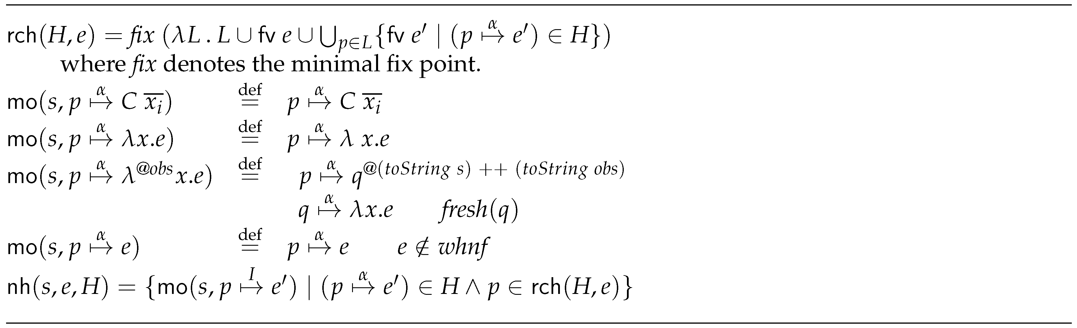
Next, we comment some implementation details of Hood that are relevant to understand how we will define appropriate semantic rules in the following sections. Hood’s implementation produce annotations of the form $(\mathit{portId},\mathit{parent},\mathit{change})$. The first component ($\mathit{portId}$) points to the place where the annotation is made. The second component ($\mathit{parent}$) is needed to know the context where an expression was evaluated. For instance, when a function is evaluated, its arguments need to know the place where they were invoked. That is, it is necessary to access to the $\mathit{parent}$ of those arguments. More precisely, parent is a tuple $(\mathit{observeParent},\mathit{observePort})$, where $\mathit{observeParent}$ is the $\mathit{portId}$ of the parent and $\mathit{observePort}$ is the position of the argument. The third parameter ($\mathit{change}$) informs about the kind of observation that is being done. It has the following possibilities:

$\mathit{Observe}\mathit{String}$ 

is created when entering in a binding that is an observation. This new observation has no parent. More precisely, its parent is the predefined general parent, denoted as $(0,0)$. As expected, when we start the evaluation of an annotated variable, this is the initial annotation that is created.

$\mathit{Enter}$ 

is created when starting the evaluation of a binding.

$\mathit{Cons}\mathit{Int}\mathit{String}$ 

is created when we evaluate a constructor. The first parameter represents the arity of the constructor, while the second one represents its name. As you might expect, the children of the constructor will receive annotations of the form $(\mathit{parentPortId},1)$, …, $(\mathit{parentPortId},\mathit{arity})$ where $\mathit{parentPortId}$ is the pointer to the $\mathit{Cons}$ annotation. By doing so, it is possible to reconstruct the constructor application.

$\mathit{Fun}$ 

is created when the binding evaluation arrives at a lambda expression. Only curryfied functions are considered, so lambda expressions have a single input value and a single result. When a lambda is applied to an input parameter, the argument is annotated with parent $(\mathit{parentPortId},0)$, while the annotation given to the result is $(\mathit{parentPortId},1)$, $\mathit{parentPortId}$ being a pointer to the $\mathit{Fun}$ annotation.

Let us remark that not only does Hood observe normal forms, it also records when an evaluation has been started. Thus, it is possible to know what binding has been demanded by other ones. When the computation finishes, the corresponding annotations are post-processed to provide the appropriate output to the user.

3. Introduction to GpH and Eden

Next, we present the basic ideas underlying the two parallel extensions of Haskell that we will use in the rest of the paper.

3.1. Glasgow Parallel Haskell

GpH [14,15,65,66] extends Haskell with simple annotations to indicate expressions that could be evaluated in parallel. It follows a thread-based approach. That is, programmers have some control to decide the parallel threads that are to be created, but they lack mechanisms to control the threads once they have been created. Threads are only handled by the underlying runtime system. The use of higher-order functions, combined with simple thread primitives, allows the programmer to create high-level abstractions. In particular, the use of evaluation strategies [65] has proven to be very useful in GpH.

The language provides two primitives for parallel (par) and sequential (seq) composition. From a denotational point of view, both primitives only return their second argument. However, from an operational point of view, e1 ‘seq‘ e2 starts forcing its first parameter (e1) to be reduced to weak head normal form, and then it starts the computation of (e2). By contrast, e1 ‘par‘ e2 first creates an annotation indicating that e1 could be evaluated using an independent parallel thread, and then it starts the computation of the second parameter. This process of annotating expressions that could be executed in parallel appears in many parallel languages, and is called the sparking of parallelism. Then, the runtime system can decide to ignore (or not) some of these annotations. That is, the programmer only suggests expressions that could be useful to be evaluated in parallel, but the runtime system manages all the low level decisions (creation of threads, synchronization, etc.).

3.2. Eden

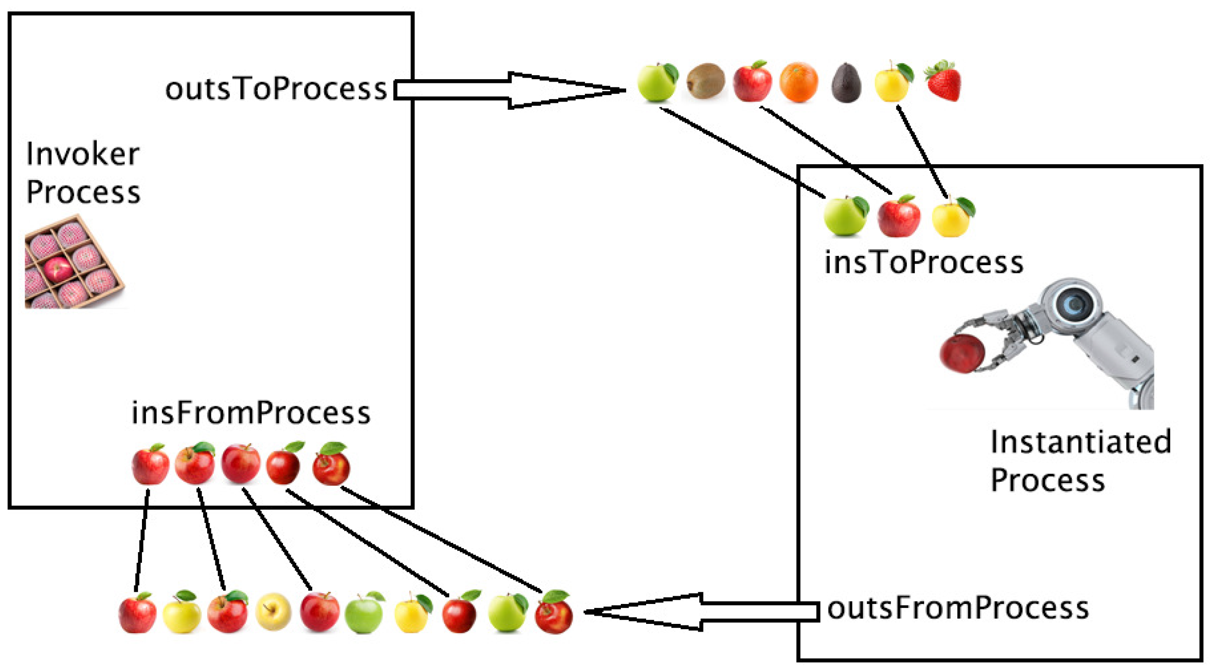
Eden [24,67,68,69] extends Haskell adding constructions to define process abstractions and to instantiate them. Any function can be transformed into a process abstraction by applying to it the predefined higher-order function process. The new process abstraction is similar to the original function it comes from, but the process abstraction can be instantiated to be executed in parallel. That is, from a semantics point of view, functions and process abstractions are analogous, the only differences appear when they are applied to their arguments. In this case, functions are applied with a function application (e1 e2), while processes are applied using a process instantiation (e1 # e2).

In Eden, a process is not a syntactical structure, it is a new computational environment that performs its computations autonomously. Each time a process instantiation (e1 # e2) takes place, the runtime system creates a new computational environment. The creator (also called parent process) of the new process will be responsible for sending the value for $e_2$ via an input channel, while the new process (also named child process or instantiated process) will receive such input value and will return to its parent (through an output channel) the result of evaluating $e_1{e}_2$.

In Eden, the communication between processes is done using pushing of information instead of pulling. That is, values are communicated even if the receiver has not demanded them (As you might expect, this rule introduces eagerness in the language. Thus, the programmer has to be careful to avoid creating unneeded work). Moreover, when a process has to send a value through one of its output channels, the corresponding values have to be fully evaluated before sending them. Streams are the only exceptions of this rule because they are sent element by element through the channels. However, each element of the stream has to be evaluated to full normal form before being transmitted. When a thread needs a value that is to be received through an input channel, and this value has not been received yet, the thread is temporarily suspended. This mechanism is the only one that can be used to synchronize Eden processes. Let us remark that the creation of processes in Eden is done explicitly, but the communication (and also the synchronization) between processes is done implicitly.

4. GpH-Eden Core Language

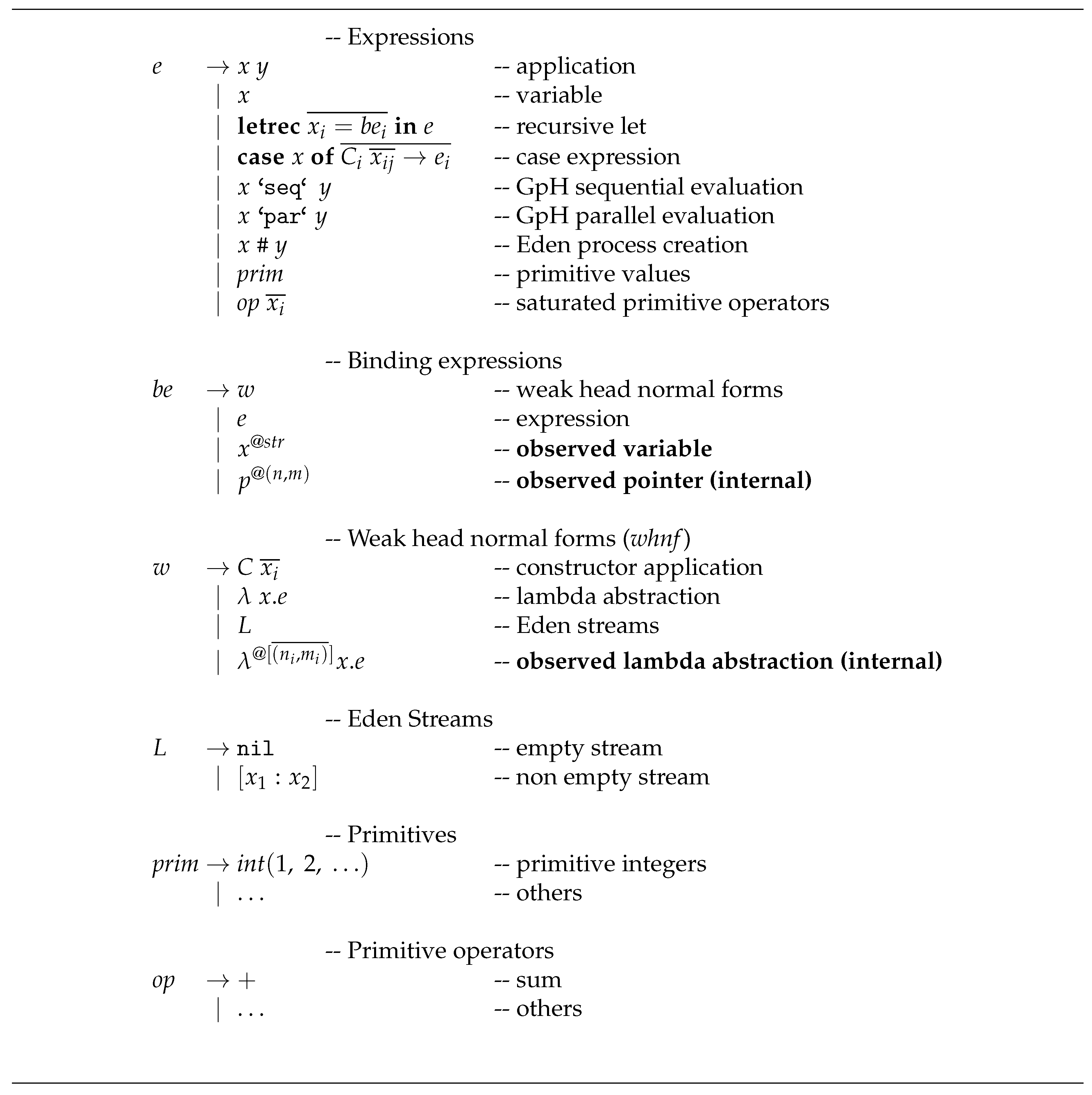
GpH and Eden are different extensions of Haskell, but they share a large part of their core languages. Thus, we will use a single framework (called GpH-Eden core) to deal with the common characteristics of both languages. The syntax of the common language can be seen in Figure 1. It is an untyped $\lambda$-calculus extended with case expressions, recursive lets, constructors application, and primitive values. It also includes expressions for the sequential and parallel compositions of GpH, as well as expressions to deal with Eden process instantiations. Any Eden or GpH expression can be translated into GpH-Eden core’s expressions by using a normalization phase. This is done by introducing the corresponding let expressions, together with the required number of intermediary variables. Regarding Eden streams, they are handled as constructors ($[x_1:x_2]$ is a constructor of arity 2, $\mathit{Cons}{x}_1{x}_2$). Thus, they can appear in case expressions. Notice that streams cannot be members of any other stream, but they can contain any other value.

Any variable can be annotated as observable by the programmer. Thus, any process abstraction can also be marked as observable. Let us remark that our core language includes two internal expressions, namely $p^{@(n,m)}$ and ${\lambda }^{@[\overline{(n_i,m_i)}]}x.e$ ($\lambda$-abstractions are annotated with a list of observers because it is possible to be observed from different points). These expressions cannot be written by the programmer. They can only appear as a result of applying other semantic rules. In this sense, they are auxiliary expressions that are useful to track who is responsible for each of the observations.

Following other classical approaches used for parallel languages (see, e.g., [64,70]), our semantics uses two levels of transition systems: the lower level is in charge of the local behavior inside each of the processes, while the upper level deals with global effects that affect several processes. In the lower level, GpH and Eden behave analogously, the only difference being that Eden does not distinguish between active and runnable threads. At a local level, the functional computations take place, such as the $\beta$-reduction, the reduction of the $\mathbf{case}$, $\mathbf{letrec}$, etc. At a global level, the global coordination behavior of the system is described with rules such as process creation, process communication, etc.

Following [64,70], we model the evaluation state of a process with a Heap: a set of bindings of variables to binding expressions. We consider that each binding can be a potential thread, and we associate a label that indicates its current state: $p\stackrel{\alpha }{\mapsto }e$, being $\alpha ::=I\left|A\right|B|R$, where the different possibilities correspond to the following meanings:

I:

Inactive. It has not been demanded yet, or its evaluation has already finished.

A:

Active. It has already been demanded and it is under evaluation.

B:

Blocked. It has been demanded, but it is currently waiting to receive a value from another binding.

R:

Runnable. It has been demanded and it is not waiting for any data, but it is not Active because it lacks an available processor.

Active and Runnable are only different in the context of GpH. The reason is that the original semantics of GpH distinguishes them, but not that of Eden. In fact, in GpH, threads are only activated in case there is an idle processor, while Eden’s scheduler is quite different in this aspect.

For the sake of conciseness, the semantic rules allow for including several labels in each binding. Each of them will represent the different possibilities that the rule admits. For instance, when $p\stackrel{IAB}{\mapsto }e$ is in the left part of a rule, while $p\stackrel{ABA}{\mapsto }{e}^{\prime }$ appears in the right part, it means that, if the thread associated with binding $p\mapsto e$ was inactive or blocked, then it becomes active. Analogously, in case it was active, then it becomes blocked. We denote by $\mathit{dom}\left(\mathit{H}\right)$ to the set that contains all the variables appearing in the left-side of any binding of the heap. Moreover, $\mathit{H}+\{p\stackrel{\alpha }{\mapsto }e\}$ represents the extension of the heap H with the binding $p\stackrel{\alpha }{\mapsto }e$. Finally, $\mathit{H}:p\stackrel{\alpha }{\mapsto }e$ indicates that the guiding binding is the one corresponding to p, that is, it is the binding that guides the application of the corresponding rule. In the previous two situations, the condition $p\notin \mathit{dom}\left(H\right)$ is assumed.

When the execution of a program e starts, $H_0=\{p_{\mathit{main}}\stackrel{A}{\mapsto }e\}$ is the starting heap, where $p_{\mathit{main}}$ is assumed to be a fresh variable (pointer). Thus, $p_{\mathit{main}}$ does not appear in e.

The meaning of $p\stackrel{B}{\mapsto }e$ is that this binding is blocked, that is, it has to wait until other computation generates certain value. We will say that expression e is blocked on a variable x, and it will be denoted by $e\in \mathsf{ble}\left(x\right)$, if it has one of the following forms $\{x,xy,\mathbf{case}x\mathbf{of}\mathit{alts},x^{@\mathit{str}},x^{@(n,m)},x‘\mathtt{seq}‘y\}$.

From now on, we will use $x,y,p,q,l,t,\mathit{ch},{\mathit{ch}}_o,{\mathit{ch}}_i\in \mathit{Var}$ for ordinary variables, $x,y$ denote program variables (written by a programmer), while $p,q,l,t$ are dynamically created free variables (that we will call pointers), ${\mathit{ch}}_i$ corresponds to input channels in Eden, ${\mathit{ch}}_o$ represents output channels, and $\mathit{ch}$ can represent any Eden channel. In the case of weak head normal forms, we will represent them using w. Moreover, in an abuse of notation, we will also use w for primitive values. The notation $\overline{P_j}$ represents that a given pattern P is repeated several times, indexing such repetitions with variable j. For instance, $\mathbf{letrec}\overline{x_i={\mathit{be}}_i}\mathbf{in}e$ will stands for $\mathbf{letrec}{x}_1={\mathit{be}}_1,\dots ,x_n={\mathit{be}}_n\mathbf{in}e$.

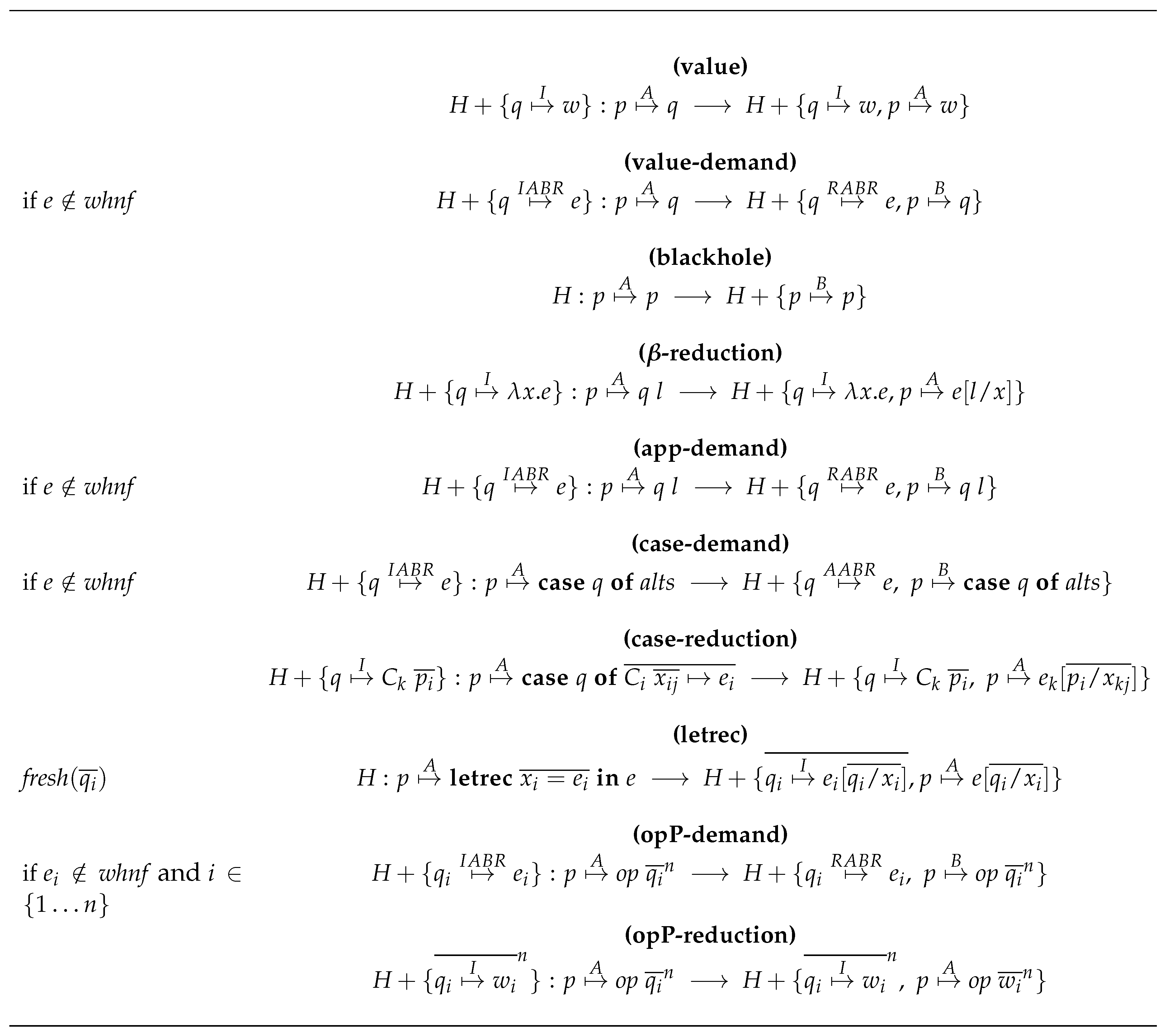
4.1. Local transitions

Local transitions are classified into two groups. The first one corresponds to ordinary expressions (see Figure 2), while the second one corresponds to Hood observations (see Figure 3). We start commenting on Figure 2, whose rules deal with the lazy evaluation of expressions. In a lazy context, if an expression is to be evaluated, it has to be demanded. This demand is represented by active bindings. That is, the guiding binding is always an active binding. A binding that is active can bind a variable to a value (meaning that the computation was already completed), to other variable, to an application, to a let-expression or to a case-expression. When a binding is active and binds a variable to other variable, there are two possibilities:

• If the two variables are equal, then we must block the corresponding variable, as we have entered a blackhole (rule blackhole).
• If the two variables are not equal, then there are two new possibilities:

  -

  When the second variable is bound to a value that has already been evaluated, we have to copy such value to the former variable (rule value).

  -

  When the second variable is bound to an expression that is not completely evaluated yet, the first variable has to be blocked (waiting until the second one is completely evaluated). Moreover, if the second variable was inactive, then it has to be turned into runnable (in the case of GpH) or into active (in the case of Eden) (rule value-demand).

Two possibilities appear when a variable is bound to an application, depending on whether the variable corresponding to its body is bound to a $\lambda$-abstraction or to a non-$\mathit{whnf}$ expression. The first situation must continue with a $\beta$-reduction (rule $\mathit{\beta }$-reduction), while, in the other situation, it is necessary to evaluate the body. That is, we turn into runnable the corresponding binding (rule app-demand).

The situation is analogous when we have to evaluate a case-expression. We have to perform the reduction when the variable is associated with a constructor (rule case-reduction), while we have to demand its evaluation in any other case (rule case-demand).

Regarding let-expressions, when we evaluate them, we have to add the corresponding new bindings (rule letrec).

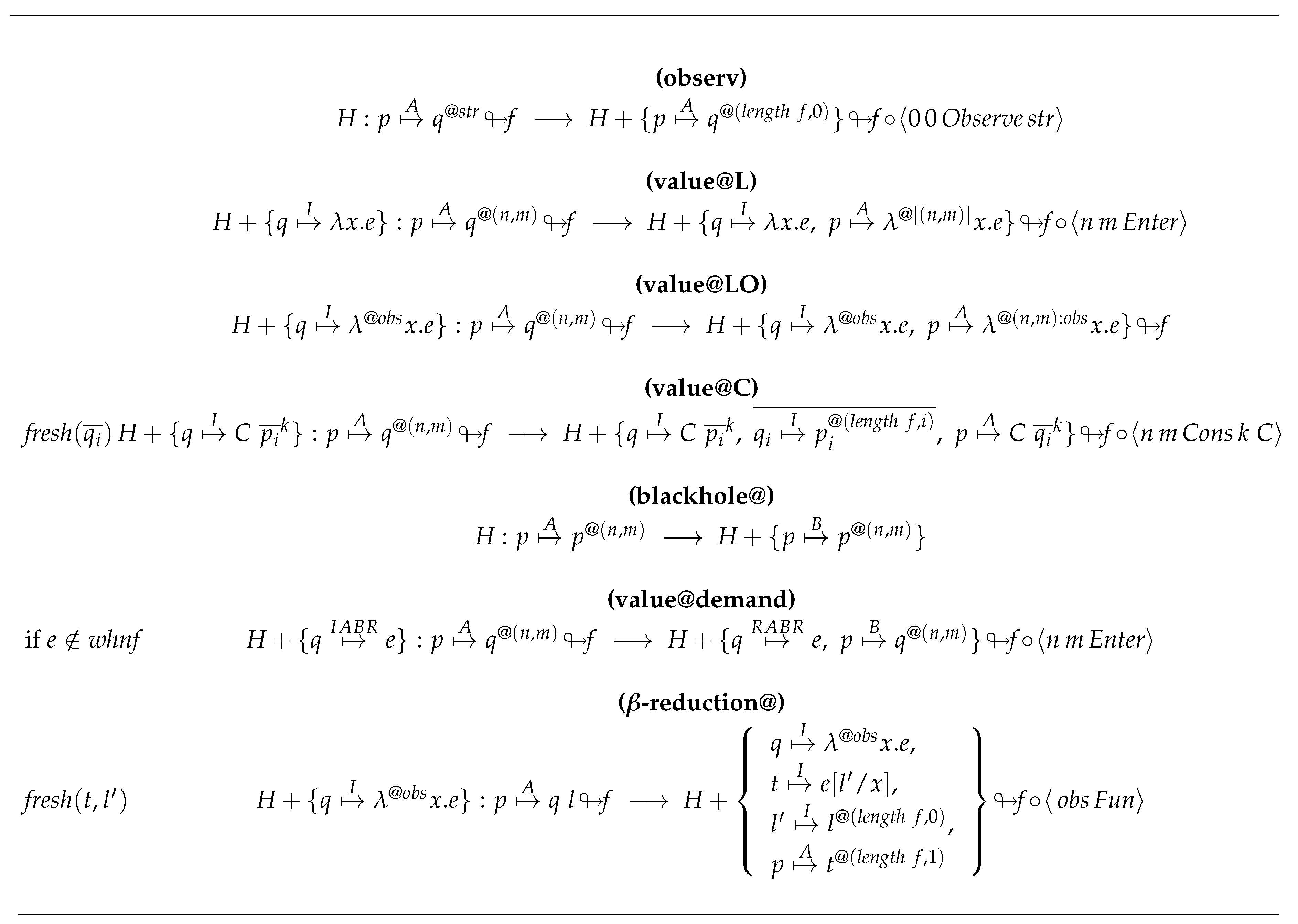
Local Rules with Observations

The rules shown in Figure 3 define the evolution of observation marks in the context of lazy evaluation. Notice that local transitions are including now a file to track the observations related to the bindings. This file will be post-processed afterwards to show the appropriate results to the user. Thus, transitions are now of the form $\mathit{H}:p\stackrel{A}{\mapsto }e\looparrowright f⟶\mathit{H}{}^{\prime }\looparrowright f^{\prime }$, meaning that the evaluation of the active thread $p\stackrel{A}{\mapsto }e$ transforms the heap $\mathit{H}+\{p\stackrel{A}{\mapsto }e\}$ into ${\mathit{H}}^{\prime }$ and adds observations to f generating a new file $f^{\prime }$. Data are always appended to the file, without modifying data previously added. Hence, $f\circ \langle \mathit{ann}\rangle$ denotes that annotation $\mathit{ann}$ has been appended to file f. Let us remark that rules in Figure 2 should also handle the corresponding files. However, for the sake of clarity, we prefer to ignore the files there because they never modify any file.

Our files will contain annotations as follows:

$$\begin{array}{ccc}\hfill \mathit{ann}& \to & \left(\mathit{observeParent}\mathit{observePort}\right)\mathit{Observe}\mathit{str}\hfill \\ & |& \left(\mathit{observeParent}\mathit{observePort}\right)\mathit{Enter}\hfill \\ & |& \left(\mathit{observeParent}\mathit{observePort}\right)\mathit{Cons}\mathit{arity}\mathit{nameConstr}\hfill \\ & |& [\overline{\left({\mathit{observeParent}}_i{\mathit{observePort}}_i\right)}]\mathit{Fun}\hfill \end{array}$$

These annotations are nearly the same as those generated by Hood, but there are two differences. First, we do not include the $portId$ corresponding to the annotation. The reason is that we can obtain this information from the line number in the file. Notice that $observeParent$ is a natural number representing the line corresponding to the annotation of the parent. Thus, $observePort$ is also a natural number. Function $\mathit{length}f$ will be used to compute the total amount of lines of the file f, 0 being the first line of the file. The second change affects the annotations of $\lambda$-abstractions: in our case, we use a list of pairs $\mathit{observeParent}$ and $\mathit{observePort}$ representing all the bindings that need to observe such $\lambda$-abstraction. This modification allows us to simplify the process of observing the same $\lambda$-abstractions from different points.

Next, we describe the observation rules:

Rule observ. 

In this case, we start an observation with the string str. Thus, an annotation $\langle 00\mathit{Observe}\mathit{str}\rangle$ is added to the file, and then the evaluation goes on, but taking into account the annotation that points to its parent, that is $(\mathit{length}f,0)$.

Rule value@L, value@LO. 

In case we deal with an active binding $p\stackrel{A}{\mapsto }{q}^{@(n,m)}$ where q is bound to a function, we have to continue evaluating a new kind of expression. If the function is previously being observed, then it is necessary to add the new observation mark to that function (rule value@LO) ${\lambda }^{@(n,m):\mathit{obs}}x.e$; otherwise, if the function has not been observed (rule value@L), then the new $\lambda$-abstraction ${\lambda }^{@[(n,m)]}x.e$ is created. This kind of lambda indicates that it is under observation associated with the tag $@[(n,m)]$. In addition, a new annotation $\langle nm\mathit{Enter}\rangle$ is generated, indicating that we enter to evaluate that binding.

Rule value@C. 

In case $q^{@(n,m)}$ is evaluated to a constructor, we have to generate a new annotation $\langle nm\mathit{Cons}kC\rangle$. This indicates that the binding whose parent is $(n,m)$ has been reduced to the constructor C (whose arity is k). New bindings pointing to each argument of that constructor are generated. These bindings are annotated to indicate that they are being observed. Moreover, in this annotation, we must indicate its position in the constructor and that its parent is in the corresponding line of the file.

Rule blackhole@. 

In this case, we have an annotated binding whose reduction needs to access to itself. Thus, we have to block the binding.

Rule value@demand. 

When dealing with a binding $p\stackrel{A}{\mapsto }{q}^{@(n,m)}$, we have to generate a new annotation $\langle nm\mathit{Enter}\rangle$ to record that we have started its evaluation.

Rule β-reduction@. 

This is the key rule to deal with the observation of functions. In case we have to evaluate an application of a function that is under observation, we generate the annotation in the file indicating that we are applying an observed function. Then, we mark its argument as observable, and we use $(\mathit{length}f,0)$ as its parent. In order to observe the result, we create a new observed binding whose parent is $(\mathit{length}f,1)$. The ports are different to remember that one is the argument and the other is the result of the lambda.

Note that it is not necessary to specify the application to an observed pointer $e{p}^{@(n,m)}$. The reason is that, in the syntax, we have restricted the places where an observed variable may appear, and in the rules we never substitute a variable by an observed pointer.

4.2. Example

Before starting to explain the specific details of each language, for the sake of clarity, we present an example. Thus, we will consider a simple example in order to see the way the observations take place.

Example 1.

We are interested in observing a single integer number but with two observations. Thus, we consider a Haskell expression as follows:

  observe "obs2" (observe "obs1" (10::Int))::Int

This expression is converted by the normalization process to a new expression ($e_0$) in our core language:

  letrec

    ten  =10

    tenO =ten@{obs1}

    tenOO=tenO@{obs2}

  in tenOO

Next, we show how this expression is reduced using our semantics. We will concentrate on the local rules, so we will not show the not yet explained global rules needed to reduce it, such as the rules concerning the activation or the blocking of the threads. In this case, as we only need one heap and one file, we will show all the steps highlighting with • the active threads that will guide the reduction. The first step corresponds to the application of theletrecrule that replaces the variables with fresh pointers: $p_1$ for ten, $p_2$ for tenO, and $p_3$ for tenOO.

$$\boxed{p_{\mathit{main}}\stackrel{A}{\mapsto }\mathbf{letrec}\dots \mathbf{in}\mathit{tenOO}}\looparrowright \left\{\begin{array}{c}\hfill \end{array}\right\}⤏$$

At this point, closure p₃ becomes active due to the application of the global rules.

   Now, adding the line numbers to the observation file we get the following file:   

$$\left\{\begin{array}{cc}Line\hfill & Observation\hfill \\ 0\hfill & 00\mathit{Observe}obs2\hfill \\ 1\hfill & 00\mathit{Enter}\hfill \\ 2\hfill & 00\mathit{Observe}obs1\hfill \\ 3\hfill & 20\mathit{Cons}010\hfill \\ 4\hfill & 00\mathit{Cons}010\hfill \end{array}\right\}$$

This file has more information than that required by Hood. In particular, the information follows the same order as the process of binding reduction. Moreover, the $\mathit{Enter}$ mark is not necessary for Hood, but this mark can provide us information about which closure was under evaluation in case of unfinished computations. Thus, the information we obtain is large enough to provide all the information required by Hood, but also all the information required by GHood [54] to produce graphical animations. Note that GHood is a graphical tool that analyzes the file and represents every annotation, for example, indicating that the closure is under evaluation when it processes an $\mathit{Enter}$ mark.

The binding corresponding to the mark obs2 ($p_3$) is the first binding under observation that is demanded. The next annotation appearing in the file means that the binding has been entered to reduce it. Before reducing this binding to normal form, $p_2$ (that is, the one annotated with obs1) has been demanded. Then, we enter to reduce this last binding, as its expression was already in normal form, an $\mathit{Enter}$ annotation for the reference $(2,0)$ has not been generated and it has immediately reached its normal form (line 3).

Now, we will show how Hood annotations can be obtained from this file. We have to generate a different observation tree for each Observe annotation in the file. To generate this tree, we start with the observations $\mathit{Observe}\mathit{str}$. Each $\mathit{Observe}\mathit{str}$ is the root of an independent tree, whose annotation is given by $\mathit{str}$. Then, it is necessary to analyze sequentially the annotations of the file. Notice that we are only interested in the marks starting with $\mathit{Cons}$: There are two of them, as it can be seen in lines 3 and 4. The former points to line 2, meaning that the parent is in line 2, while the later points to line 0. Hence, two trees are obtained:

Then, we only have to flatten the previous trees to produce the same output that Hood produces:

--obs1

      10

--obs2

      10

5. GpH Formal Semantics

When we evaluate a GpH core expression, we will usually need to create several independent threads. However, we will only need one heap because GpH core does not have processes, communication, etc.

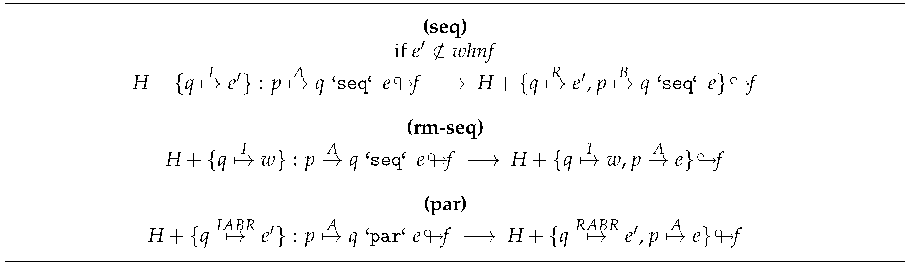
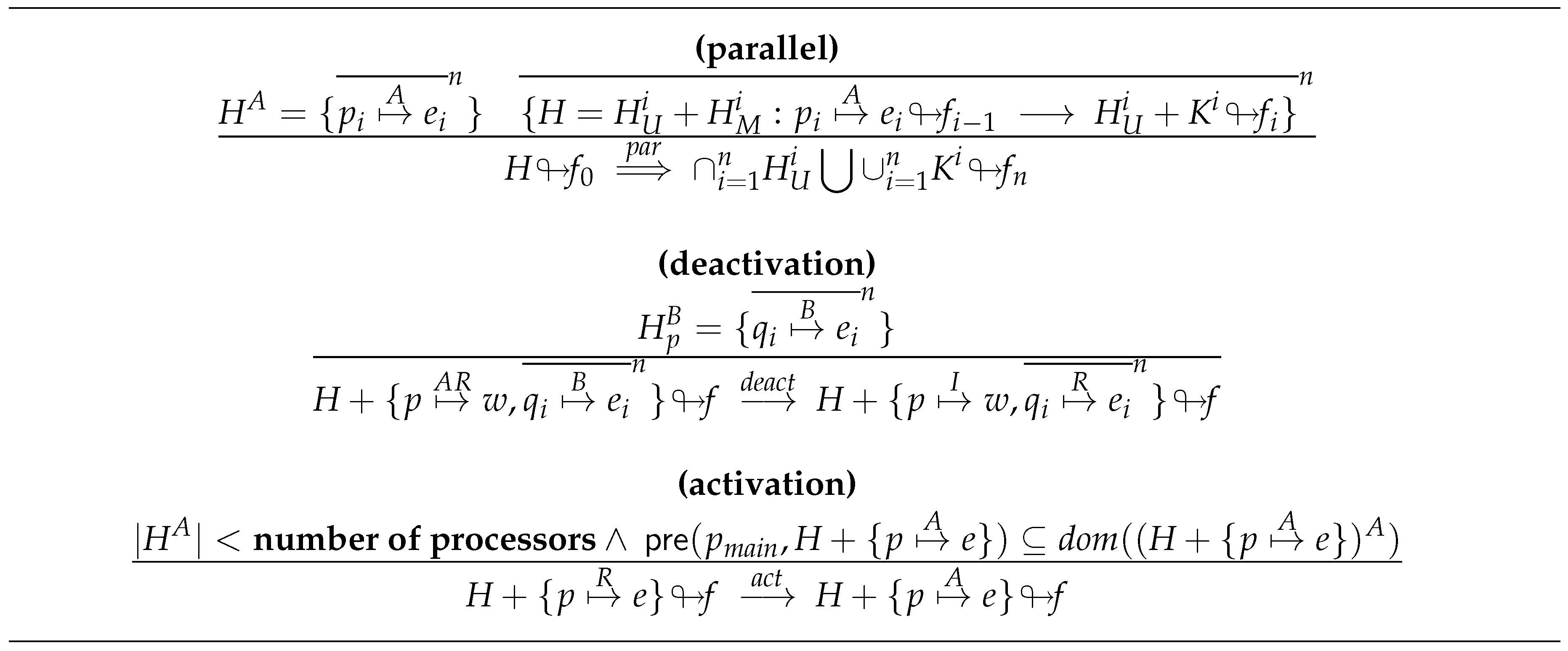
The semantics has been divided in two parts: The rules corresponding to the local behavior of the GpH operators ($‘\mathtt{seq}‘$ and $‘\mathtt{par}‘$) can be seen in Figure 4, and the ones defining the global behavior of GpH are shown in Figure 5. First, let us comment the first set of rules. In case the left variable is not yet reduced to $\mathit{whnf}$, the sequentiality of the $‘\mathtt{seq}‘$ operator forces its evaluation (rule seq). After obtaining the value, we proceed with the evaluation of the second variable (rule rm-seq). Regarding the $‘\mathtt{par}‘$ operator, it creates a potential thread. If p points to a $‘\mathtt{par}‘$ binding, we have to go on with the evaluation of its second parameter. Moreover, the binding corresponding to the first parameter becomes runnable (denoting that it can be a new thread), provided that it wasn’t demanded yet (rule par).

5.1. GpH Global transitions

Let us start introducing some notation. The global rules define named transitions of the form $\stackrel{\diamond }{⟶}$, where ⋄ corresponds to the name of some rule. In addition, the meaning of $\stackrel{\diamond }{⟹}$ is that rule $\stackrel{\diamond }{⟶}$ has to be applied as many times as possible. Moreover, $\stackrel{\diamond }{⟹}\circ \stackrel{\square }{⟹}$ represents the composition of rules ⋄ and □: First, the rule □ is applied and afterwards the rule ⋄. The local evolution of the system depends on the threads that are active in H, and we represent this set as ${\mathit{H}}^A$:

$${\mathit{H}}^A=\{(p\stackrel{A}{\mapsto }\mathit{be})|(p\stackrel{A}{\mapsto }\mathit{be})\in \mathit{H}\}$$

and $|{\mathit{H}}^A|$ is its cardinal. Following the same notation, the threads blocked on p are represented as ${\mathit{H}}_p^B$:

$${\mathit{H}}_p^B=\{(q\stackrel{B}{\mapsto }\mathit{be})|(q\stackrel{B}{\mapsto }\mathit{be})\in \mathit{H}\wedge \mathit{be}\in \mathsf{ble}\left(p\right)\}$$

Now, we will discuss the global transitions of the GpH semantics. First of all, let us remark that GpH has a single common heap for all threads. Thus, the introduction of the annotation file in the rules is quite straightforward, as this file will be shared by all threads under execution. Next, we comment on the rules dealing with the global behavior (Figure 5):

Rule parallel 

Each thread that is active can evolve independently (using local rules), and then we have to merge the corresponding heaps to obtain the global behavior. More precisely, we have to consider each active thread $p_i\stackrel{A}{\mapsto }{e}_i$. Then, for each one, we consider two parts of the heap $\mathit{H}={\mathit{H}}_U^i+{\mathit{H}}_M^i$, where ${\mathit{H}}_U^i$ contains those bindings that are not modified by the local rules, while ${\mathit{H}}_M^i$ contains those bindings that were modified by the evolution of the thread, and their final state after such evolution is represented by ${\mathit{K}}^i$. The final heap contains those parts that were not modified by any thread ${\cap }_{i=1}^n{\mathit{H}}_U^i$, together with the result of the execution of the threads ${\cup }_{i=1}^n{\mathit{K}}^i$. In order to consider this rule, it is necessary to prove that all the involved heaps are consistent, that is, there is no interference between the evolution of the active bindings. This proof can be found in [71].

We print the observations in sequence: We start with $f_0$ and then we continue printing the annotations coming from the evaluation of thread $p_1\stackrel{A}{\mapsto }{e}_1$; next, we go on with those corresponding to thread $p_2\stackrel{A}{\mapsto }{e}_2$; later, we continue with those of $p_3\stackrel{A}{\mapsto }{e}_3$, and so on.

Let us remark that different evaluation orders among threads can result in different files. However, all of the possible files are consistent with the observations. In fact, we could even modify the rule to mimic the concurrent evaluation of the threads. The only restriction is that a semaphore has to be used to access the file, so that we can guarantee that the printing operations are atomic.

Rule deactivation 

In this case, we do not transform the annotation file. The rule turns into runnable those bindings that were previously blocked on a pointer, provided that this pointer is now bound to a value. Moreover, the pointer has to turn into inactive mode.

Rule activation 

As in the previous case, the rule does not transform the annotation file. There can be as many active threads as available processors, and this number is a global constant. Thus, it is not possible to always turn any runnable thread into an active thread, and it is necessary to define a priority criterion. In particular, GpH gives priority to those variables that are currently demanded by the main thread. More precisely, the preference criterion $\mathsf{pre}(p_{\mathit{main}},\mathit{H})$ is the following:

$$\mathsf{pre}(p,\mathit{H})=\left\{\begin{array}{cc}p,\hfill & \mathrm{if}p\stackrel{AR}{\mapsto }e\in \mathit{H}\hfill \\ \mathsf{pre}(q,\mathit{H}),\hfill & \mathrm{if}p\stackrel{B}{\mapsto }e\in \mathit{H}ande\in \mathsf{ble}\left(q\right)\hfill \end{array}\right.$$

Global evolution comprises a scheduling phase that consists of deactivation and the activation of threads:

$$\stackrel{\mathit{sched}}{⟹}=\stackrel{\mathit{act}}{⟹}\circ \stackrel{\mathit{deact}}{⟹}$$

Finally, the global evolution is defined as follows:

$$⟹=\stackrel{\mathit{sched}}{⟹}\circ \stackrel{\mathit{par}}{⟹}$$

First, all the rules concerning the parallel evolution are applied, and then the scheduling evolution takes place.

5.2. Example: Semantic Evaluation in GpH

In order to better understand the behavior of the observations in GpH, let us provide an example of the semantic evaluation of a GpH expression. In this example, we will concentrate on the reduction steps corresponding to the observations. For that, we will show the interaction between the observation marks and the parallel computation.

Example 2.

In this example, we will observe the Fibonacci function: We will evaluate a parallel version of this function with an observation mark. The parallelism will be achieved because the arguments of the function will be evaluated in parallel. Notice that the observations will also be produced in parallel, due to both recursive calls of the parfibO. We will present here only the rules corresponding to observations and parallel computations.

We will reduce the Fibonacci of 2 that will be enough to understand the parallel evolution. We will consider that we have two processors to produce the reduction. The initial GpH expression is the following:

main=parfibO 2

parfibO=observe "parfib" parfib

parfib::Int ->Int

parfib 0=1

parfib 1=1

parfib n=nf2 ‘par‘ (nf1 ‘seq‘ (nf1+nf2))

           where nf1=parfibO (n-1)

                 nf2=parfibO (n-2)

After the normalization process, the corresponding expression in our language is $e_0$:

  letrec

    one   = 1

    two   = 2

    parfib  = \n. case n of

               0 -> one

               1 -> one

               _ -> letrec

                            n1= - n one

                            n2= - n two

                            nf1= parfibO n1

                            nf2= parfibO n2

                            sum= + nf1 nf2

                            sol= nf1 ‘seq‘ sum

                        in   nf2 ‘par‘ sol

    parfibO = parfib@parfib

  in parfibO two

Notice that n corresponds to an unboxed integer. Let us recall that the integers are considered ordinary constructors of arity 0. To present the examples, we consider that $\mathbf{case}$ expressions have a default alternative “_” meaning that we are not interested in the value of n. The starting configuration is the following:

$$\boxed{p_{\mathit{main}}\stackrel{A}{\mapsto }\mathbf{letrec}\dots \mathbf{in}\mathrm{parfib}0\mathrm{two}}\looparrowright \left\{\begin{array}{c}\hfill \end{array}\right\}⤏$$

At this point, there is only one active thread under execution. It will evolve until new threads are created.

After the next step (just below), we have reached the point where $p_6$ points to the $‘\mathtt{par}‘$ expression. At this point, two threads are generated, corresponding with the reduction of the $‘\mathtt{par}‘$ expression $p_6$. The main thread becomes blocked and two new active threads are created ($p_6$ and $p_{10}$).

At this point, the parallel evolution of the two new threads starts. The evolution of the thread $p_{10}$ will produce the following configurations:

At this moment, the parallel rule activates the threads $p_{12}$ and $p_{14}$. This activation produces a demand on the bindings $p_9$ and $p_{13}$; these bindings become active after a new application of rule parallel. Now, two new observations are produced: One corresponding to a reduction applying the $\mathit{\beta }$-reduction@ rule to the binding $p_9$, and another one corresponding to the application of the demand@ rule to the binding $p_{13}$. These observations might have been produced in a different order, although one can easily check that the final observations would have been the same. These reductions correspond to the following configurations:

After these reductions, the rule demand@ is applied to the binding $p_9$. This rule produces another observation in the observation file, and it activates the bindings $p_8$ and $p_{16}$. Next, the activation rule is applied to the bindings $p_8$ and $p_{16}$. These steps are presented here:

Now, the rule demand@ is applied in parallel to the bindings $p_{13}$ and $p_{15}$. The evaluation of both threads in parallel will generate the following configurations:

At this point, the evaluation of the binding $p_{10}$ finishes, but the computations must continue evaluating the only thread under execution: $p_{16}$.

The computation ends at this point. Thus, the produced annotation file will contain the following observations:

$$\left\{\begin{array}{cc}Line\hfill & Observation\hfill \\ 0\hfill & 00\mathit{Observe}parfib\hfill \\ 1\hfill & [(00)]\mathit{Fun}\hfill \\ 2\hfill & 11\mathit{Enter}\hfill \\ 3\hfill & 10\mathit{Cons}02\hfill \\ 4\hfill & [(00)]\mathit{Fun}\hfill \\ 5\hfill & 41\mathit{Enter}\hfill \\ 6\hfill & [(00)]\mathit{Fun}\hfill \\ 7\hfill & 40\mathit{Enter}\hfill \\ 8\hfill & 61\mathit{Enter}\hfill \\ 9\hfill & 40\mathit{Cons}00\hfill \\ 10\hfill & 60\mathit{Enter}\hfill \\ 11\hfill & 60\mathit{Cons}01\hfill \\ 12\hfill & 41\mathit{Cons}01\hfill \\ 13\hfill & 61\mathit{Cons}01\hfill \\ 14\hfill & 11\mathit{Cons}02\hfill \end{array}\right\}$$

By analyzing this file, we can generate the following observation tree:

The flattening of the tree will produce the following observation:

-- parfib

  { \ 2 -> 2

  , \ 1 -> 1

  , \ 0 -> 1

  }

6. Eden Formal Semantics

When we evaluate an Eden core expression, it can be necessary to create many parallel processes, where each of them encompasses several independent threads. In particular, each thread will be in charge of evaluating one of the outputs that the process has to produce. The input values of the process are given by its parent at the moment of its creation, and this input data are shared by all the threads within the process. The threads trying to access to unevaluated inputs are temporarily blocked. Let us recall that the instantiation of processes is done explicitly, while any other aspect (like communication or synchronization) is carried out implicitly. Eden allows two kinds of communications: transmitting a value in a single piece, or using stream-based communication. First, we will only deal with single value communication; and, later, we will give the rules for stream-based communication.

Figure 2 and Figure 3 show the rules dealing with the local behavior in Eden. It is only important to highlight that we do not distinguish between active and runnable threads. That is, we assume that labels A and R are equal.

In contrast to the case of GpH, now there is not a single heap. An independent heap is used for each process, and they do not share bindings among them. Thus, it will be easier to use independent files to handle the observations of each process. Thus, a process is now denoted by $\langle \mathit{id},\mathit{H}\looparrowright f\rangle$, where $id$ is the identifier of the process, H represents the heap, and f denotes the corresponding file of observations.

6.1. Eden Global transitions

We will use the global transition rules to manage how the processes evolve in parallel. The basic aspect of a global transition is as follows:

$$\{\overline{\langle r,{\mathit{H}}_r\rangle \looparrowright f_r}\}\stackrel{\diamond }{⟶}\{\overline{\langle r,{\mathit{H}}_r^{\prime }\rangle \looparrowright f_r^{\prime }}\}$$

Notice that the heap of each process r (that is, ${\mathit{H}}_r$) can change into a new heap ${\mathit{H}}_r^{\prime }$. Moreover, the transition can also create new processes. Furthermore, the observation file of each process ($f_r$) can also be modified, adding new annotations and producing a new file $f_r^{\prime }$.

6.1.1. Auxiliary Functions

A few auxiliary functions will be useful to simplify the definition of our global rules:

Function $\mathsf{nh}$. 

Each process has its own heap, without sharing bindings with other processes. Thus, when a new process is created, we have to copy from the parent heap to the new heap all the bindings that will be necessary to evaluate the process body. Function $\mathsf{nh}$ (needed heap, see Figure 6) will be used to tackle this issue. In particular, $\mathsf{nh}(s,e,\mathit{H})$ gathers those bindings of $\mathit{H}$ that can be reached from e. Moreover, it also transforms the observation marks in all the closures adding them the string s. During the process of cloning bindings between heaps, care has to be taken when we find a lambda abstraction that is under observation (notice that they are the only $\mathit{whnf}$ that can be under observation). In this case, it is important to record its original process. We will achieve this by modifying the observation associated with the binding. Function $\mathsf{mo}(s,p\mapsto e)$ (modify observations) deals with this problem. Notice that it only has to consider the definition for $\mathit{whnf}$ forms. Nevertheless, there exist different options to define this modification:

• As it appears in Figure 6. The observations are modified to remember where they come from, that is, which is the corresponding parent.
• Not modifying the observations and simply copying them to the new heap ($\mathsf{mo}(\mathit{id},p\stackrel{\alpha }{\mapsto }{\lambda }^{@\mathit{obs}}x.e)=p\stackrel{\alpha }{\mapsto }{\lambda }^{@\mathit{obs}}x.e$). In this way, it is not possible to get the relations between the observations produced in the child and in the parent. Nevertheless, by post-processing the annotation files, it is possible to rebuild these relations.
• A third option consists of removing the observation marks of all the bindings ($\mathsf{mo}(\mathit{id},p\stackrel{\alpha }{\mapsto }{\lambda }^{@\mathit{obs}}x.e)=p\stackrel{\alpha }{\mapsto }\lambda x.e$). In this way, the observations are only produced in the process that starts the evaluation of the observation mark. Thus, in case programmers are interested in observing some data in the child process, it is necessary that they explicitly introduce an observation mark in the body of the process.

Function $\mathsf{nff}$. 

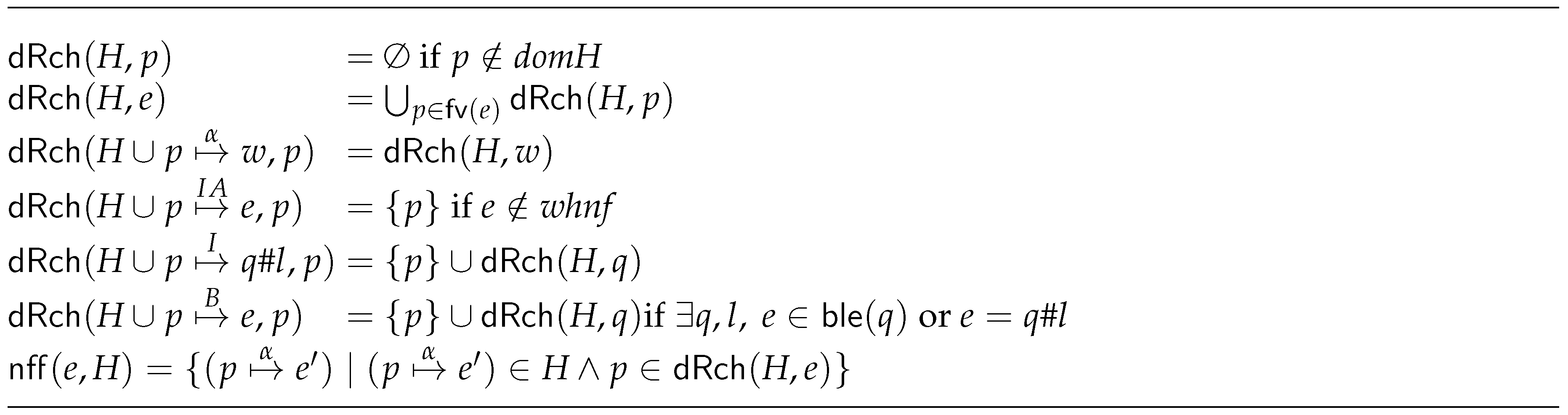
Every time a process is created or communication between processes takes place, it is necessary to guarantee that any expression that is sent is in $\mathit{whnf}$. This is done recursively. That is, in case a pointer appears in an expression, then we have to follow such pointer and guarantee that the expression it is pointing at is also in $\mathit{whnf}$. Function needed first free ($\mathsf{nff}$, see Figure 7) checks this condition, and it returns those reachable expressions that are not in $\mathit{whnf}$. Thus, if we look at the process creation rules, we see that we can only create process q with heap H provided that $\mathsf{nff}(q,H)=\varnothing$. Analogously, we need $\mathsf{nff}(e,H)=\varnothing$ to be able to send e in a heap H (value communication demand rule). Function $\mathsf{nff}$ will also appear in rule process creation demand. In this case, it provides the bindings that are needed to perform the eager creation of the new process.

6.1.2. Global Rules

After introducing the necessary notation, we will comment on the rules concerning the global evolution of Eden. At this level, we need to tackle the following issues: process creation (Figure 8), inter-process communication (Figure 9), thread management (Figure 10), and the actual system evolution (Figure 11). For each of them, several steps will be needed to obtain the required behavior, and they will typically require to handle two processes. In order to keep the rules simple, we do not show the observation files in those rules that never modify it. Moreover, let us remind that the rules can only transfer the file from the left to the right part of the rule.

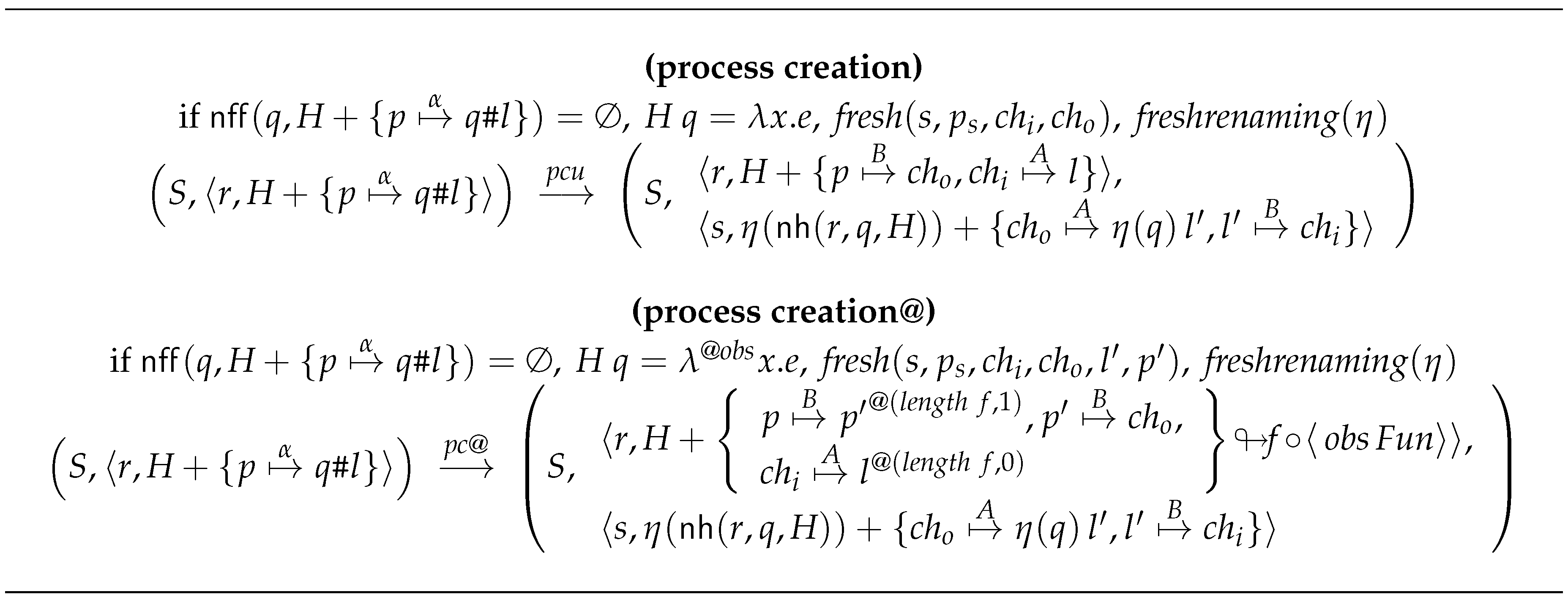
Process creation. 

The creation of a new process takes place when an #-expression is evaluated. In this case, we have to apply a rule from Figure 8. In case the process is under observation, we use rule process creation@, while rule process creation is used otherwise.

Analogously to the case of the definition of $\mathsf{nh}$ function, there exist different options for the process creation rule:

• To create the new process without taking into account if the process is an observed $\lambda$-abstraction or not. In this way, the rule process creation@ would not be necessary. It is only necessary to consider that the body of the process in process creation rule can be an observed $\lambda$-abstraction. This $\lambda$-abstraction will be modified by the function $\mathsf{nh}$; so, the observations obtained will depend on the version of $\mathsf{nh}$ that we use.
• To create the new process taking into account that the process can be an observed $\lambda$-abstraction. In this case, we will observe the input and output channels. The rule process creation@ indicates this behavior. As in the previous case, the $\lambda$-abstraction will be modified by the function $\mathsf{nh}$; and the observations will depend on the choice of $\mathsf{nh}$.

In any case, when we create a new process, we create a new output channel ${\mathit{ch}}_o$ and we have to block on it the parent thread that evaluated the #-expression. This channel corresponds to the initial thread in the new child process s and it will be used to communicate the final value from the child to the parent. Analogously, on the child side, a thread will be blocked on a new input channel ${\mathit{ch}}_i$; this channel is controlled by a new thread in the parent and it will be used for sending data from the parent to the child. As we have already mentioned, the creation of processes is not lazy. In fact, a process is instantiated as soon as we find in the heap a variable that points directly to a #-expression, no matter if the binding is currently active or not.

Both rules are equal in all aspects but one: The second rule needs to introduce observations in the data exchanged with the process. Let us remark that the annotations in process r are handled in the same way as the observation of a $\lambda$-abstraction.

We define the iteration of these rules as:

$$\stackrel{\mathit{pc}}{⟹}=\stackrel{\mathit{pc}@}{⟹}\circ \stackrel{\mathit{pcu}}{⟹}$$

Inter-processes communication. 

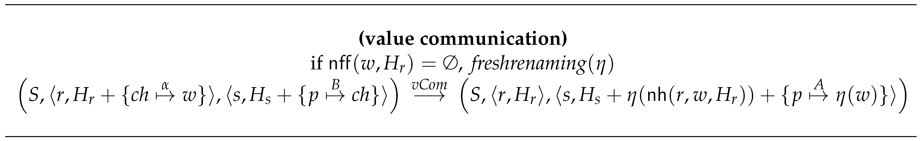
Figure 9 deals with the communication of values. Let us remind that in order to send a value we have to copy (from the heap of the sender to the heap of the receiver) the bindings of the variables that can be reached from such value. The situation is the same as when we were creating a new process, that is, we can only proceed with the rule in case the expressions to be copied are in $\mathit{whnf}$($\mathsf{nff}(w,{\mathit{H}}_r)=\varnothing$). We need to avoid name repetitions in the heap of the child process. Thus, we apply an $\eta$–rename to everything in $\mathsf{nh}(r,w,{\mathit{H}}_r)$. Then, the multi-step rule dealing with communication is defined as follows: $\stackrel{\mathit{Com}}{⟹}=\stackrel{\mathit{vCom}}{⟹}$. Let us remark that the rule appearing in Figure 9 deals with the communication of a single value. Later, in Section 6.3, we will extend the semantics so that it can deal with stream communication.

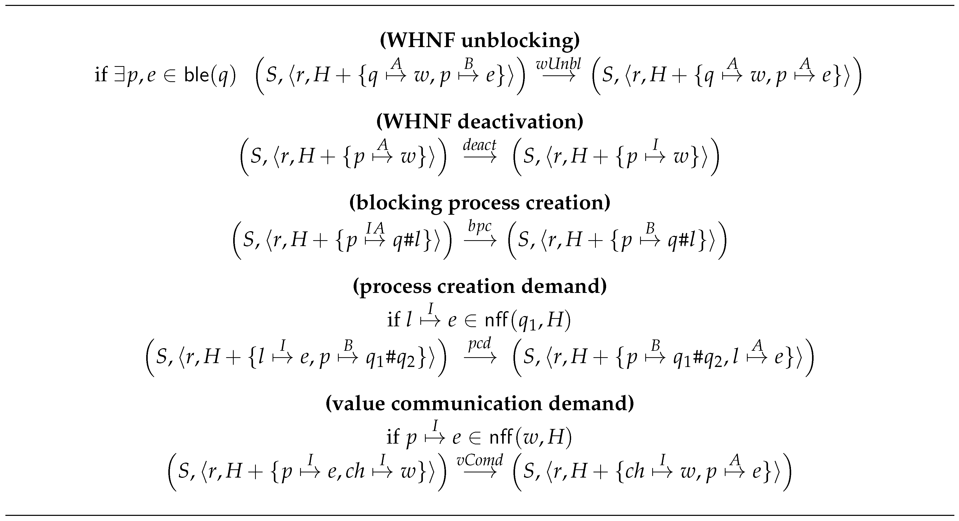
Thread management. 

Figure 10 contains the rules dealing with the management of the threads. The aim of each one is the following:

WHNF unblocking: 

When a binding finally reaches its final value (it is a $\mathit{whnf}$), the threads blocked on it are unblocked.

WHNF deactivation: 

Another operation that must be performed is the deactivation of the bindings that have reached their final value.

Blocking process creation: 

The creation of new processes must be blocked until their free dependencies are in $\mathit{whnf}$.

Process creation demand: 

In order to be able to unblock the recently created processes, the evaluation of their needed free variables must be demanded.

Value communication demand: 

In order to be able to communicate a value through a channel, it must be in $\mathit{whnf}$, so its evaluation must be demanded.

Finally, let us recall the previous rules activate the application of rules value and app-demand.

By combining and iterating rules from Figure 10, we obtain the following rule:

$$\stackrel{\mathit{Unbl}}{⟹}=\stackrel{\mathit{vComd}}{⟹}\circ \stackrel{\mathit{pcd}}{⟹}\circ \stackrel{\mathit{bpc}}{⟹}\circ \stackrel{\mathit{deact}}{⟹}\circ \stackrel{\mathit{wUnbl}}{⟹}.$$

It is trivial to prove that Unbl always finishes. That is, these rules can only be applied a finite number of times. The reason is that the amount of threads that are blocked cannot be infinite, and its number cannot be increased by using a deactivation or an unblock.

System evolution rules. 

The overall behavior of the system is governed by these rules. Each process evolves by using local transitions, and then the global system evolves. Figure 11 gathers this behavior: Rule parallel-r deals with the local evolution inside a process, while the overall evolution is done with parallel that handles all processes in a single rule.

The internal evolution of each process is done following the local rules shown in Section 4.1. Thus, the internal evolution of process r depends on the active threads in $H_r$ that can evolve. Notice that parallel-r is the equivalent to the rule parallel that was defined for GpH. The difference is that in Eden there is an independent heap for each process. Thus, the number of active threads belonging to process r is $n_r=\left|H_r^A\right|$.

After defining how each process evolves, rule parallel defines how the whole system S evolves.

6.1.3. Global System Evolution

Once we have defined how each process evolves, we need to tackle the evolution of the overall system. We use $⟹$ to represent it. Its definition is as follows:

$$⟹=\stackrel{\mathit{sys}}{⟹}\circ \stackrel{\mathit{par}}{⟹}$$

We defined $\stackrel{\mathit{par}}{⟹}$ in rule parallel. Now, we can define $\stackrel{\mathit{sys}}{⟹}$ as follows:

$$\stackrel{\mathit{sys}}{⟹}=\stackrel{\mathit{Unbl}}{⟹}\circ \stackrel{\mathit{pc}}{⟹}\circ \stackrel{\mathit{Com}}{⟹}$$

Transition $\stackrel{\mathit{sys}}{⟹}$ indicates that all pending communications must be performed, next we create new processes, and then we deal with thread management.

Finally, a computation is an evolution of the global system:

$$S_0⟹S_1⟹\dots$$

We consider that the computation finishes when the $p_{\mathit{main}}$ pointer is inactive. However, there are more options to consider the end of a computation such as there are not any active threads in the system.

6.1.4. Semantic Possibilities

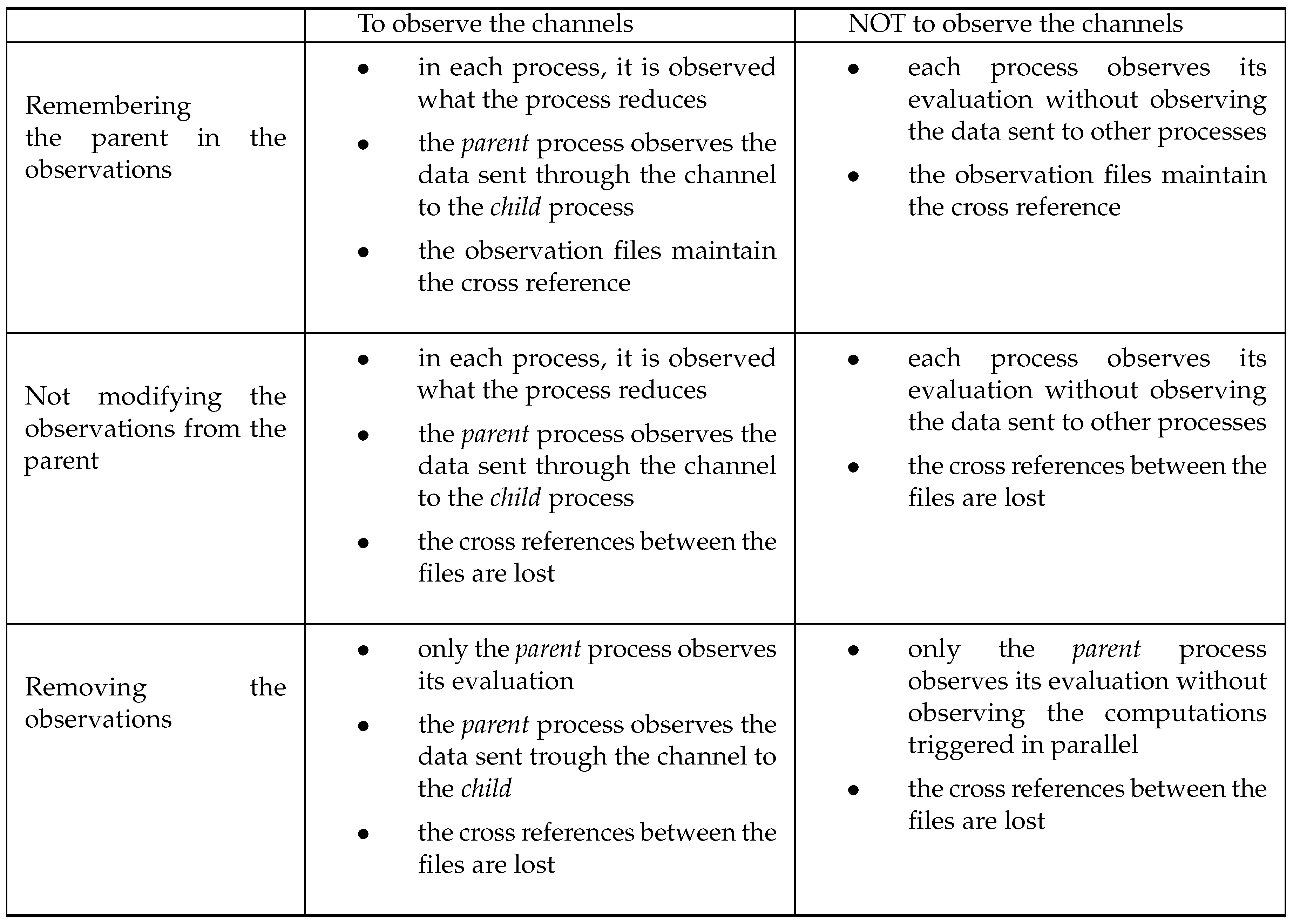
As we have discussed previously, there are several options to define the process creation rule (two alternatives) and the definition of the function $\mathsf{mo}$ (three options). Since both features are independent, we have up to six possibilities to define the formal semantics with respect to the observations. The selection of any of these possibilities will affect to the observations we get in the annotation file. Thus, when analyzing the final results, we must be aware of the semantic option we are considering.

The table in Figure 12 summarizes these semantic possibilities. In this table, we want to remark that the richest option with respect to the observations is the one that chooses to observe the channels in the process creation rule and to remember the parent in the $\mathsf{mo}$ function. The fewer observations are obtained in the semantic option that chooses not to observe the channels in the process creation rule and to remove the observations in the $\mathsf{mo}$ function. The rest of the cases just lay in the middle of both alternatives.

6.2. Example: Semantic Evaluation in Eden

As in the case of the GpH semantics, now we present an example to illustrate the behavior of the semantics we have just defined. For that, we will show the interactions between the parallel computation and the reduction of the observation marks. It will also be interesting to analyze the different semantic options because this will clarify the advantages and disadvantages of each alternative.

Example 3.

We are going to consider the same example we used to illustrate the GpH semantics: The parallel computation of the Fibonacci function. In this way, we can also see the differences at the semantic level between Eden and GpH. Again, we are going to compute in parallel the recursive calls of the Fibonacci function.

As in the GpH example, we will reduce the Fibonacci of 2 that will be representative enough to analyze the parallel evolution. Thus, the starting expression in Eden is:

main=parfibO~2

 

parfibO=observe "parfib" (process parfib)

 

parfib::Int ->Int

parfib 0=1

parfib 1=1

parfib n=(parfibO#(n-1))+(parfibO#(n-2))

that yields, after the normalization process, the initial expression $e_0$:

  letrec

    one   = 1

    two   = 2

 

    parfib  = \n. case n of

                    0 -> one

                    1 -> one

                    _ -> letrec

                                 n1= - n one

                                 n2= - n two

                                 nf1=parfibO # n1

                                 nf2=parfibO # n2

                             in  + nf1~nf2

 

    parfibO = parfib@{parfib}

  in parfibO two

Again, we will consider that $\mathbf{case}$ expressions have a default alternative _ meaning that the actual value of n is not relevant. Next, we will present the most important reductions from the initial configuration:

$$\boxed{p_{\mathit{main}}\stackrel{A}{\mapsto }\mathbf{letrec}\dots \mathbf{in}\mathrm{parfib}\mathrm{O}\mathrm{two}}\looparrowright \left\{\begin{array}{c}\hfill \end{array}\right\}$$

Up to this point, the computation has been similar to the one produced in GpH. Now, the parallel computation begins and the evolution differs from the one we have shown for GpH in Example 2. At this point, the semantic rules indicate that two processes must be created to compute the bindings $p_9$ and $p_{10}$ in parallel.

A new heap for each of the new processes is built. These heaps will be different depending on the semantic option we are considering. For each of the semantic options we have described, we will show the resulting annotation files.

1. 

Observing the channels and modifying the observation marks adding that they came from the other process (such as is presented in the semantic rules, Figure 8):

This is the richest semantics in terms of observations in the annotation files. First, the rules indicate that two new processes (child 1 and child 2) must be created. Thus, two new heaps are built, each one contains the information needed by the process. We also create the communication channels. On the one hand, we have the bindings corresponding to the output parent channels (the variables $c{h}_{13}$ and $c{h}_{21}$), the corresponding bindings are blocked in the parent process and active in the offspring. On the other hand, we have input parent channels (${\mathit{ch}}_{12}$ and ${\mathit{ch}}_{20}$) that are active in the parent process and blocked in the child processes.

More precisely, each process is the application of the Fibonacci function (parfibO) to the corresponding parameters. Thus, the first task that must be accomplished is to copy all the needed heap to compute this function into the child processes. Since it is an observed λ-abstraction, the rule process creation@ is applied. In the table below, the heaps of the three processes just after the application of this rule can be found.

Since we are using the version of the function $\mathsf{mo}$ that modifies the observations, we get bindings with the observations modified: [main, (0 0)] . Note that rule process creation@ makes an annotation in the file of the parent process as if it were a function. Thus, lines 4 and 5 of the parent annotation file (in the table below) are produced at this moment.

Then, all three of the processes evolve independently until the child processes are blocked because they need the argument of the Fibonacci function. This value has to be computed in the parent process. During this autonomous evolution, annotations are produced in the annotation files. The parent process has to evaluate the parameters needed by the child processes, and this evaluation generates the lines 6–9 in the parent process file. The child processes begin their execution and as result we obtain lines 0–2 in their respective files.

At this point, the child processes can no longer continue until they communicate with the parent process, so the value communication rule is applied. After that, the child processes continue and generate lines 3–4 in their respective annotation files. Now that the resulting values have just been computed in the child processes, they can be sent back to the parent process by using again the rule value communication. In addition, finally the parent process makes the annotation in lines 10–12 in its file. In the table below, we show all the annotations we have described:

$$\boxed{\begin{array}{ccc}main\hfill & child1\hfill & child2\hfill \\ \left\{\begin{array}{cc}Line\hfill & Observation\hfill \\ 0\hfill & 00\mathit{Observe}parfib\hfill \\ 1\hfill & [(00)]\mathit{Fun}\hfill \\ 2\hfill & 11\mathit{Enter}\hfill \\ 3\hfill & 10\mathit{Cons}02\hfill \\ 4\hfill & [(00)]\mathit{Fun}\hfill \\ 5\hfill & [(00)]\mathit{Fun}\hfill \\ 6\hfill & 50\mathit{Enter}\hfill \\ 7\hfill & 40\mathit{Enter}\hfill \\ 8\hfill & 40\mathit{Cons}01\hfill \\ 9\hfill & 50\mathit{Cons}00\hfill \\ 10\hfill & 41\mathit{Cons}01\hfill \\ 11\hfill & 51\mathit{Cons}01\hfill \\ 12\hfill & 11\mathit{Cons}02\hfill \end{array}\right\}\hfill & \left\{\begin{array}{cc}Line\hfill & Observation\hfill \\ 0\hfill & 00\mathit{Observe}[main,(00)]\hfill \\ 1\hfill & [(00)]\mathit{Fun}\hfill \\ 2\hfill & 11\mathit{Enter}\hfill \\ 3\hfill & 10\mathit{Cons}00\hfill \\ 4\hfill & 11\mathit{Cons}01\hfill \end{array}\right\}\hfill & \left\{\begin{array}{cc}Line\hfill & Observation\hfill \\ 0\hfill & 00\mathit{Observe}[main,(00)]\hfill \\ 1\hfill & [(00)]\mathit{Fun}\hfill \\ 2\hfill & 11\mathit{Enter}\hfill \\ 3\hfill & 10\mathit{Cons}01\hfill \\ 4\hfill & 11\mathit{Cons}01\hfill \end{array}\right\}\hfill \end{array}}$$

Analyzing each file independently, we can obtain the following observation trees:

main	child 1	child 2

These trees can be flattened to be shown to the user as:

main	child 1	child 2
-- parfib    { \ 2 -> 2    , \ 1 -> 1    , \ 0 -> 1    }	-- [main, parfib]    { \ 0 -> 1    }	-- [main, parfib]    { \ 1 -> 1    }

2. 

Observing the channels and not modifying the observations:

In this case, the differences appear when the rule process creation@ is applied because now it is only necessary to copy the needed heap from the parent process (applying an η renaming). The main difference with respect to the previous case is that the bindings $p_{15}$ and $p_{23}$ are not created, and the bindings $p_{14}$ and $p_{22}$ will be bound to the expression ${\lambda }^{@[(0,0)]}n.\mathbf{case}\mathit{n}\mathbf{of}\mathit{alts}$. Then, proceeding like in the previous case, we get that the final observations appearing in the files are the following:

$$\boxed{\begin{array}{ccc}main\hfill & child1\hfill & child2\hfill \\ \left\{\begin{array}{cc}Line\hfill & Observation\hfill \\ 0\hfill & 00\mathit{Observe}parfib\hfill \\ 1\hfill & [(00)]\mathit{Fun}\hfill \\ 2\hfill & 11\mathit{Enter}\hfill \\ 3\hfill & 10\mathit{Cons}02\hfill \\ 4\hfill & [(00)]\mathit{Fun}\hfill \\ 5\hfill & [(00)]\mathit{Fun}\hfill \\ 6\hfill & 50\mathit{Enter}\hfill \\ 7\hfill & 40\mathit{Enter}\hfill \\ 8\hfill & 40\mathit{Cons}01\hfill \\ 9\hfill & 50\mathit{Cons}00\hfill \\ 10\hfill & 41\mathit{Cons}01\hfill \\ 11\hfill & 51\mathit{Cons}01\hfill \\ 12\hfill & 11\mathit{Cons}02\hfill \end{array}\right\}\hfill & \left\{\begin{array}{cc}Line\hfill & Observation\hfill \\ 0\hfill & [(00)]\mathit{Fun}\hfill \\ 1\hfill & 01\mathit{Enter}\hfill \\ 2\hfill & 00\mathit{Cons}00\hfill \\ 3\hfill & 01\mathit{Cons}01\hfill \end{array}\right\}\hfill & \left\{\begin{array}{cc}Line\hfill & Observation\hfill \\ 0\hfill & [(00)]\mathit{Fun}\hfill \\ 1\hfill & 01\mathit{Enter}\hfill \\ 2\hfill & 00\mathit{Cons}01\hfill \\ 3\hfill & 01\mathit{Cons}01\hfill \end{array}\right\}\hfill \end{array}}$$

Thus, we obtain the following observation trees:

main	child 1	child 2

In addition, they produce the following observations:

main	child 1	child 2
-- parfib    { \ 2 -> 2    , \ 1 -> 1    , \ 0 -> 1    }	--    { \ 0 -> 1    }	--    { \ 1 -> 1    }

As we can observe, in this case, the annotations of the child processes that refer to the parent process are missing.

3. 

Observing the channels and removing the observations when the bindings are copied into another process:

Now, the differences with respect to the previous case is that $p_{14}$ and $p_{22}$ will be bound to a non-observed expression $\lambda n.\mathbf{case}\mathit{n}\mathbf{of}\mathit{alts}$. Thus, we do not get any observations in the corresponding files of the child processes. Therefore, the final annotation files will be the following:

$$\boxed{\begin{array}{ccc}main\hfill & child1\hfill & child2\hfill \\ \left\{\begin{array}{cc}Line\hfill & Observation\hfill \\ 0\hfill & 00\mathit{Observe}parfib\hfill \\ 1\hfill & [(00)]\mathit{Fun}\hfill \\ 2\hfill & 11\mathit{Enter}\hfill \\ 3\hfill & 10\mathit{Cons}02\hfill \\ 4\hfill & [(00)]\mathit{Fun}\hfill \\ 5\hfill & [(00)]\mathit{Fun}\hfill \\ 6\hfill & 50\mathit{Enter}\hfill \\ 7\hfill & 40\mathit{Enter}\hfill \\ 8\hfill & 40\mathit{Cons}01\hfill \\ 9\hfill & 50\mathit{Cons}00\hfill \\ 10\hfill & 41\mathit{Cons}01\hfill \\ 11\hfill & 51\mathit{Cons}01\hfill \\ 12\hfill & 11\mathit{Cons}02\hfill \end{array}\right\}\hfill & \left\{\begin{array}{c}\hfill \end{array}\right\}\hfill & \left\{\begin{array}{c}\hfill \end{array}\right\}\hfill \end{array}}$$

Then, showing the observations in a tree form, we get:

main	child 1	child 2

In addition, the corresponding observations are as follows:

main	child 1	child 2
-- parfib    { \ 2 -> 2    , \ 1 -> 1    , \ 0 -> 1    }

4. 

Not observing the channels and modifying the observation marks adding the process they come from: In this case (and in the following ones), when the child processes are created, the rule process creation will be used, even if the function that is going to be executed in the child process is under observation. The difference with respect to case 1 is that the channels are under observation (as indicated in rule process creation). Thus, the bindings of pointers $p_9$ and $p_{10}$ are bounded directly with its corresponding channels ${\mathit{ch}}_{13}$ and ${\mathit{ch}}_{21}$, and the channels ${\mathit{ch}}_{12}$ and ${\mathit{ch}}_{20}$ are directly bounded to $p_7$ and $p_8$ (without any observation marks). Then, proceeding as in the previous cases, the resulting annotation files are:

$$\boxed{\begin{array}{ccc}main\hfill & child1\hfill & child2\hfill \\ \left\{\begin{array}{cc}Line\hfill & Observation\hfill \\ 0\hfill & 00\mathit{Observe}parfib\hfill \\ 1\hfill & [(00)]\mathit{Fun}\hfill \\ 2\hfill & 11\mathit{Enter}\hfill \\ 3\hfill & 10\mathit{Cons}02\hfill \\ 4\hfill & 11\mathit{Cons}02\hfill \end{array}\right\}\hfill & \left\{\begin{array}{cc}Line\hfill & Observation\hfill \\ 0\hfill & 00\mathit{Observe}main[(10)]\hfill \\ 1\hfill & [(00)]\mathit{Fun}\hfill \\ 2\hfill & 01\mathit{Enter}\hfill \\ 3\hfill & 00\mathit{Cons}00\hfill \\ 4\hfill & 01\mathit{Cons}01\hfill \end{array}\right\}\hfill & \left\{\begin{array}{cc}Line\hfill & Observation\hfill \\ 0\hfill & 00\mathit{Observe}main[(10)]\hfill \\ 1\hfill & [(00)]\mathit{Fun}\hfill \\ 2\hfill & 01\mathit{Enter}\hfill \\ 3\hfill & 00\mathit{Cons}01\hfill \\ 4\hfill & 01\mathit{Cons}01\hfill \end{array}\right\}\hfill \end{array}}$$

Whose tree representation is:

main	child 1	child 2

Thus, the final observations are as follows:

main	child 1	child 2
-- parfib   { \ 2 -> 2    }	-- [main parfib]   { \ 0 -> 1   }	-- [main parfib]    { \ 1 -> 1    }

This case is similar to case 1, the difference being that the data transmitted through the channels are not observed. In every process, the λ-abstraction applications that have been reduced locally are only obseved.

5. 

Not observing the channels and not modifying the observations:

In this case, bindings $p_{15}$ and $p_{23}$ are created, and bindings $p_{14}$ and $p_{29}$ will be bound to the expression ${\lambda }^{@[(0,0)]}n.\mathbf{case}\mathit{n}\mathbf{of}\mathit{alts}$. Thus, the final observation files produced in the global computation will be the following:

$$\boxed{\begin{array}{ccc}main\hfill & child1\hfill & child2\hfill \\ \left\{\begin{array}{cc}Line\hfill & Observation\hfill \\ 0\hfill & 00\mathit{Observe}parfib\hfill \\ 1\hfill & [(00)]\mathit{Fun}\hfill \\ 2\hfill & 11\mathit{Enter}\hfill \\ 3\hfill & 10\mathit{Cons}02\hfill \\ 12\hfill & 11\mathit{Cons}02\hfill \end{array}\right\}\hfill & \left\{\begin{array}{cc}Line\hfill & Observation\hfill \\ 0\hfill & [(00)]\mathit{Fun}\hfill \\ 1\hfill & 01\mathit{Enter}\hfill \\ 2\hfill & 00\mathit{Cons}00\hfill \\ 3\hfill & 01\mathit{Cons}01\hfill \end{array}\right\}\hfill & \left\{\begin{array}{cc}Line\hfill & Observation\hfill \\ 0\hfill & [(00)]\mathit{Fun}\hfill \\ 1\hfill & 01\mathit{Enter}\hfill \\ 2\hfill & 00\mathit{Cons}01\hfill \\ 3\hfill & 01\mathit{Cons}01\hfill \end{array}\right\}\hfill \end{array}}$$

Again, analyzing each file we get the following observation trees:

main	child 1	child 2

In addition, the produced observations are as follows:

main	child 1	child 2
-- parfib    { \ 2 -> 2    }	--    { \ 0 -> 1    }	--    { \ 1 -> 1    }

The main difference with respect to the previous case is that the references to the parent process are missing in the child process annotations.

6. 

Not observing the channels and removing the observations when the bindings are copied into the child process:

In this case, bindings $p_{14}$ and $p_{22}$ will be directly bound to the unobserved expression $\lambda n.\mathbf{case}\mathit{n}\mathbf{of}\mathit{alts}$. Therefore, the child processes will not produce any kind of observations. This implies that the observation files after the computation will be the following:

$$\boxed{\begin{array}{ccc}main\hfill & child1\hfill & child2\hfill \\ \left\{\begin{array}{cc}Line\hfill & Observation\hfill \\ 0\hfill & 00\mathit{Observe}parfib\hfill \\ 1\hfill & [(00)]\mathit{Fun}\hfill \\ 2\hfill & 11\mathit{Enter}\hfill \\ 3\hfill & 10\mathit{Cons}02\hfill \\ 4\hfill & 11\mathit{Cons}02\hfill \end{array}\right\}\hfill & \left\{\begin{array}{c}\hfill \end{array}\right\}\hfill & \left\{\begin{array}{c}\hfill \end{array}\right\}\hfill \end{array}}$$

Thus, their tree representations are:

main	child 1	child 2

In addition, the corresponding observations are as follows:

main	child 1	child 2
-- parfib    { \ 2 -> 2    }

As it can be seen in the previous example, the most complete option is the one that uses the rule process creation@ and the complete $\mathsf{mo}$ function. Unfortunately, this option requires introducing changes in the Haskell compiler to implement it that would break the modularity of Hood (it is one of its most interesting features). Thus, in our current implementation (see [61]), we have decided to use rule process creation@ but with the intermediate option for function $\mathsf{mo}$. That is, in order to keep our implementation simple, we are not recording all the possible information, but we are quite close to obtaining all the information. In fact, by using adequate annotations and by postprocessing the results, we can obtain nearly the same information.

6.3. Eden Streams

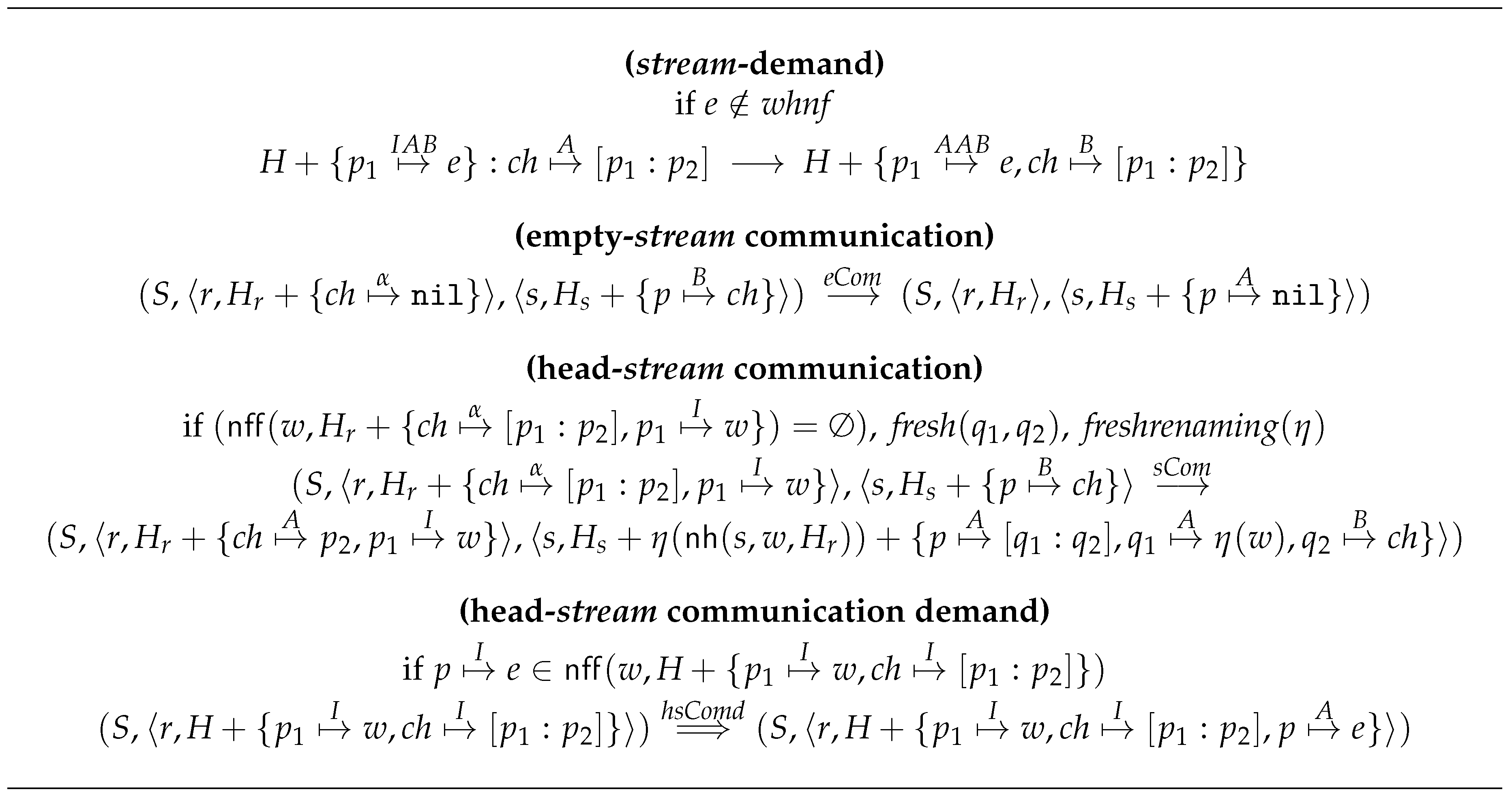
In the rules we have introduced so far, processes communicate only a single value through any channel. Of course, this single value could be a list, but in order to send this list it should be in normal form, which would prevent sending many of the interesting structured data that can be defined in a lazy language. In order to allow for communicating more than a value through the channel, Eden has streams, a structure similar to lists that allows for sending a list of values through a channel, sending them one at a time, and as soon as they are available. In order to handle streams, we need the rules in Figure 13: one new local rule (stream-demand), two new global communication rules (empty-stream communication and head-stream communication) and one new global demand communication rule (head-stream communication demand). Let us remark that the observation file is not modified by any of these rules.

We explain them briefly:

stream-demand.

If a channel deals with streams, and we have not yet evaluated the head of the stream, we demand it. The reason is that Eden streams are evaluated eagerly.

empty-streamcommunication.

If the stream is finished (that is, it is $\mathtt{nil}$), we send such value and then we close the stream. Thus, it will not be possible to perform any other communication using the channel.

head-streamcommunication.

When the head of a stream is available to be sent, the receiver gets a fresh variable with the corresponding value. This communication is similar to the one of the value communication rule.

head-streamcommunication demand.

If the head of the stream is evaluated to $\mathit{whnf}$, then we have to demand its needed first free bindings.

Let us remark that any communication can allow new communications to take place. Hence, we have to repeat the applications of rules value communication, empty-stream communication, and head-stream communication until no further communication is possible. Thus, we define

$$\stackrel{\mathit{Com}}{⟶}=\stackrel{\mathit{vCom}}{⟹}\circ \stackrel{\mathit{eCom}}{⟹}\circ \stackrel{\mathit{sCom}}{⟹}$$

and then $\stackrel{\mathit{Com}}{⟹}$ as usual. It is also necessary to modify the $\stackrel{\mathit{Unbl}}{⟹}$ rule by adding the rule head-stream communication demand:

$$\stackrel{\mathit{Unbl}}{⟹}=\stackrel{\mathit{hsComd}}{⟹}\circ \stackrel{\mathit{vComd}}{⟹}\circ \stackrel{\mathit{pcd}}{⟹}\circ \stackrel{\mathit{bpc}}{⟹}\circ \stackrel{\mathit{deact}}{⟹}\circ \stackrel{\mathit{wUnbl}}{⟹}.$$

6.4. Stream Communication in Eden via an Example

Next, we will present an example of communication using Eden streams. In this example, we will also present a problem that will be studied in more detail in Section 8: Speculative computations. In order to speed up the computation, Eden communications are performed eagerly, that is, the data to be communicated must be computed even if there is not demand for those data. This implies that some unneeded computations could be performed.

Example 4.

In this example, the parent process creates a child process that generates an infinite list. The parent process will only use the second element of this list, so the child process may compute many non-demanded values. The concrete expression we are going to show is the following:

main = elemI 2 (lFromNO # 7)

 

lFromNO = observe "lFromN"~lFromN

 

lFromn :: int -> [Int]

lFromn n = n:lFromn (n + 1)

 

elemI ::Int ->[a] ->a

elemI 1 (x:xs)=x

elemI n (x:xs)=elemI (n-1) xs

After the normalization process, the expression we have to compute in our language is $e_0$:

  letrec

    one   = 1

    two   = 2

    seven = 7

 

    elemI  = \n\ys. case n of

                1 -> case ys of

                       Cons x xs -> x

                _ -> case ys of

                 Cons x xs -> letrec

                                       n1= - n one

                                       elemN1= elemI n1

                                    in  elemN1~xs

 

    lFromn  = \n. letrec

                n1= + n one

                lns= lFromn n1

             in (n : lns)

 

    lFromNO = lFromN@{lFromN}

 

    instEden = lFromNO # seven

    elemTwo = elemI~two

 

  in elemTwo instEden

The reduction of the $\mathbf{letrec}$ expression will produce the following configuration:

At this moment, due to the rule process creation@, the reduction of $p_6$ needs to create the child process. After that, the computation reaches the following configuration:

This is the point where the parallel computation starts in Eden. Due to the rules stream–demand and head–stream demand, the child begins to produce results. When the child produces a new result, it will be transmitted according to the rule head–stream communication. The next configuration is produced after the application of the rule stream–demand that produces a demand on the head of the stream:

In order to communicate a value, it is necessary that all reachable bindings from $p_6$ are in $\mathit{whnf}$. Thus, we reach the following configuration:

Now, according to the rule head–stream communication, the value computed in the child process is communicated and we reach the following configuration:

The computation continues. Note that the child and the parent are not synchronized. Thus, while the parent is making its computation, the child could be able to produce data even if they are not demanded by the parent, that is, speculative work can be done. In this example, we will suppose that the child process generates two extra data before the computation ends. The global computation ends when the parent gets all the data it needs and it finishes its own computation; then, it sends a kill signal to the child process.

$$\boxed{\begin{array}{cc}main\hfill & child\hfill \\ \left\{\begin{array}{cc}Line\hfill & Observation\hfill \\ 0\hfill & 00\mathit{Observe}lFromN\hfill \\ 1\hfill & [(00)]\mathit{Fun}\hfill \\ 2\hfill & 10\mathit{Cons}07\hfill \\ 3\hfill & 11\mathit{Cons}2:\hfill \\ 4\hfill & 31\mathit{Cons}2:\hfill \\ 5\hfill & 40\mathit{Cons}08\hfill \end{array}\right\}\hfill & \left\{\begin{array}{cc}Line\hfill & Observation\hfill \\ 0\hfill & 00\mathit{Observe}main[(10)]\hfill \\ 1\hfill & [(00)]\mathit{Fun}\hfill \\ 2\hfill & 11\mathit{Enter}\hfill \\ 3\hfill & 11\mathit{Cons}2:\hfill \\ 4\hfill & 30\mathit{Enter}\hfill \\ 5\hfill & 10\mathit{Cons}07\hfill \\ 6\hfill & 30\mathit{Cons}07\hfill \\ 7\hfill & 31\mathit{Enter}\hfill \\ 8\hfill & 31\mathit{Cons}2:\hfill \\ 9\hfill & 80\mathit{Enter}\hfill \\ 10\hfill & 80\mathit{Cons}08\hfill \\ 11\hfill & 81\mathit{Enter}\hfill \\ 12\hfill & 81\mathit{Cons}2:\hfill \\ 13\hfill & 120\mathit{Enter}\hfill \\ 14\hfill & 120\mathit{Cons}09\hfill \\ 15\hfill & 121\mathit{Enter}\hfill \\ 16\hfill & 121\mathit{Cons}2:\hfill \\ 17\hfill & 160\mathit{Enter}\hfill \\ 18\hfill & 160\mathit{Cons}010\hfill \\ 19\hfill & 161\mathit{Enter}\hfill \\ 20\hfill & 161\mathit{Cons}2:\hfill \end{array}\right\}\hfill \end{array}}$$

By analyzing each file, we obtain the following observation trees:

That can be flattened to obtain the following observation:

-- lFromN   { \ 7 -> _ : 8 : _   }

-- main[(1 0)]   { \ 7 -> 7 : 8 : 9 : 10 : _ : _   }

Analyzing these observations, we can extract the following conclusions:

• The parent did not need the first value sent from the child to compound the final result.
• The child has produced two extra numbers, 9 and 10 that the parent did not need to get its final result.

In general, the programmers can have difficulty with finding by their own this unneeded computations. However, once a tool points out the situation, it is not difficult to modify the program to overcome this problem. In Section 8, we illustrate how we can easily obtain information about unneeded work in Eden.

7. Correctness and Equivalences

One key aspect of Hood is that the observations should not modify the meaning of any expression. Thus, any time we evaluate an annotated expression, the result should be equal to the result obtained when we evaluate the equivalent expression without annotations. In addition to that, it is necessary to prove that the expressions that are demanded now are exactly the same as in the evaluation of the original non-observed expression.

Obviously, observation marks are the main differences. Hence, we define a function that removes them, so that we will be able to compare expressions with and without observations. The transformation removing the observations from any GpH-Eden core’s expression is defined next.

Definition 1.

Function $\mathsf{R}:GpH-Edencore⟶GpH-Edencore$ removes observations. Its definition is done recursively, and the only case that is not straightforward appears when we find an observed expression:

$$\begin{array}{ccc}\mathsf{R}{x}^{@\mathit{str}}\hfill & \stackrel{def}{=}& x\hfill \\ \mathsf{R}{p}^{@(r,s)}\hfill & \stackrel{def}{=}& p\hfill \\ \mathsf{R}{\lambda }^{@\mathit{obs}}x.e\hfill & \stackrel{def}{=}& \lambda x.\mathsf{R}e\hfill \end{array}$$

We can trivially extend the previous definition to remove all the observations of a heap, since we only have to apply $\mathsf{R}$ to all the expressions appearing in the Heap. Thus, $\mathsf{R}\mathit{H}$ means $\{p\mapsto \mathsf{R}e\mid (p\mapsto e)\in \mathit{H}\}$.

The theorem we want to prove states that, if we evaluate an expression with observation marks, the final result is the same as if we remove the observation marks from the expression. The first problem we have to address is defining what we understand by the final result. Since we are working with a lazy language, it is not enough to consider the final value of the expression, we have to guarantee that we have not introduced eagerness into the evaluation. Thus, we need a stronger result that the final heap in both cases is the same. Formally, we would like to prove the following property For all $e\in$ GpH core:

$$\{p_{\mathit{main}}\stackrel{A}{\mapsto }\mathsf{R}e\}\looparrowright \langle \rangle ⟹\mathit{H}\looparrowright \langle \rangle \mathrm{iff}\{p_{\mathit{main}}\stackrel{A}{\mapsto }e\}\looparrowright \langle \rangle ⟹\mathit{H}\looparrowright f$$

Unfortunately, this property does not hold. The problem is that in the rules with observations we introduce auxiliary pointers to deal with observations, for instance rule $\mathit{\beta }$-reduction@ adds two new pointers to the heap (t and $l^{\prime }$); these new pointers do not have an exact equivalent in the corresponding rule without observations: $\mathit{\beta }$-reduction. These new pointers point to the original ones, but they have marks to remind that we are observing them. Thus, instead of proving that they are equal, we will prove that both expressions are essentially the same. We would like to define a simulation relation between heaps $\mathit{H}⊑{\mathit{H}}^{\prime }$ such that $\forall (p\stackrel{\alpha }{\mapsto }e)\in \mathit{H}$ the equivalent binding $(p^{\prime }\stackrel{\alpha }{\mapsto }{e}^{\prime })\in {\mathit{H}}^{\prime }$ has the same value as e in $\mathit{H}$, that is, if we follow all the pointers, we will finally find the same expressions. To establish the simulation relation between the heaps, it is necessary to take into account the state of the threads. That is, when we are evaluating an expression without observations, if the corresponding thread is active and the reduction of an equivalent expression with observation marks has intermediate pointers, the state of one of these pointers will be active; moreover, the previous intermediate pointers will be blocked as they will be waiting the result of the thread, and the posterior intermediate threads will be inactive. When the state of the binding without observations is inactive or blocked, then the intermediate pointers in the equivalent expression with observation marks will be inactive or blocked, respectively. Finally, when the state of the binding without observations is runnable, then the first or the last intermediate pointers in the equivalent expression with observation marks will be runnable. If it is the first, then the rest will be inactive and if it is the last then the rest will be blocked waiting the final result. The following definition establishes that simulation relation, where $\mathit{rp}e$ corresponds to the obvious function that removes pointers from the original expression, so that expressions can be comparable.

Definition 2.

Let $\mathit{H},{\mathit{H}}^{\prime }$ be two heaps. We say that:

• $\mathit{H}⊑{\mathit{H}}^{\prime }$ if $\exists \eta -rename$, $\forall (p\stackrel{\beta }{\mapsto }e)\in \mathit{H}$ then $\exists n\in IN,\{{\overline{q_i\stackrel{{\alpha }_i}{\mapsto }{q}_{i+1}}}^{n-1},q_n\stackrel{{\alpha }_n}{\mapsto }{e}^{\prime }\}$ where $\eta p=q_1$ and the following conditions holds:

  -

  $\mathit{rp}e{⊑}_{\mathsf{R}}\mathit{rp}{e}^{\prime }$

  -

  and one of the following conditions holds:

  ∗

  if $\beta =A$ then $\exists k\in \{1\dots n\}$, ${\alpha }_k=A$, $\forall j\in \{1\dots k-1\}$, ${\alpha }_j=B$ and $\forall j\in \{k+1\dots n\}$, ${\alpha }_j=I$.

  ∗

  if $\beta =I$ then $\forall j\in \{1\dots n\}$, ${\alpha }_j=I$.

  ∗

  if $\beta =B$ then $\forall j\in \{1\dots n\}$, ${\alpha }_j=B$.

  ∗

  if $\beta =R$ then one of the following conditions holds:

  ·

  ${\alpha }_1=R$ and $\forall j\in \{2\dots n\}$, ${\alpha }_j=I$

  ·

  ${\alpha }_n=R$ and $\forall j\in \{1\dots n-1\}$, ${\alpha }_j=B$

• $\mathit{H}{⊑}_{\mathsf{R}}{\mathit{H}}^{\prime }$ if $\mathit{H}⊑\mathsf{R}{\mathit{H}}^{\prime }$

First, we present a proof about the equivalence in GpH of the evaluation of observed and unobserved expressions. Then, we will deal with the analogous proof for the case of Eden. Let us remind that all GpH threads share a common heap.

Theorem 1.

For any $e\in$ GpH core we have:

$$\{p_{\mathit{main}}\stackrel{A}{\mapsto }\mathsf{R}e\}\looparrowright \langle \rangle ⟹\mathit{H}\looparrowright \langle \rangle iff\{p_{\mathit{main}}\stackrel{A}{\mapsto }e\}\looparrowright \langle \rangle ⟹{\mathit{H}}^{\prime }\looparrowright f$$

$$and\mathit{H}{⊑}_{\mathsf{R}}{\mathit{H}}^{\prime }$$

We can prove it taking into account the ideas presented in [72]. Thus, first we consider a generalization of Theorem 1, as shown in the following proposition.

Proposition 1.

Let $\mathit{H}$ be one heap without observation marks, ${\mathit{H}}^{*}$ one heap such that $\mathit{H}{⊑}_{\mathsf{R}}{\mathit{H}}^{*}$, and f a file, then:

$$\mathit{H}⟹\mathit{K}iff{\mathit{H}}^{*}\looparrowright f⟹{\mathit{K}}^{*}\looparrowright f^{\prime }$$

$$and\mathit{K}{⊑}_{\mathsf{R}}{\mathit{K}}^{*}$$

Proof. 

All the technical details of the proof can be seen in the Appendix A. Next, we present the main scheme of the proof.

We will prove it by induction on the derivation. First, it is necessary to prove that the local rules with observations produce equivalent configurations to the local rules without observations. To prove this, in some cases, it is needed to apply more than one rule in the evaluation of an expression with observation marks, while it will be needed to apply only one rule in the equivalent heap without observation marks. Regarding local transitions, the only difference is that in GpH we can use $‘\mathtt{seq}‘$ and $‘\mathtt{par}‘$, but observations do not affect them. Thus, local rules preserve the equivalence.

The proof has to pay special attention to rule $\mathbf{parallel}$ because the annotation file is not modified by rules $\mathbf{activation}$ and $\mathbf{deactivation}$. The difficulty with rule $\mathbf{parallel}$ comes when we have to perform ${\cup }_{i=1}^n{\mathit{K}}^i$. In this case, we have to take care of possible conflicts between observed pointers. In fact, we prove the absence of interferences in the case of GpH. That is, in case there are bindings in heaps ${\mathit{K}}^j$ and ${\mathit{K}}^k$ for the same pointer p, then the value is equal. That is, if $(p\stackrel{\alpha }{\mapsto }{e}_j)\in {\mathit{K}}^j$ and $(p\stackrel{\beta }{\mapsto }{e}_k)\in {\mathit{K}}^k$, then $\alpha =\beta$ and $e_j=e_k$. Regarding observations, one heap could have two bindings $(p\stackrel{\alpha }{\mapsto }{q}^{@(n_1,n_2)})\in {\mathit{K}}^j$ and $(p\stackrel{\alpha }{\mapsto }{q}^{@(n_1^{\prime },n_2^{\prime })})\in {\mathit{K}}^k$. That means $(p\stackrel{A}{\mapsto }{q}^{@\mathit{str}})\in \mathit{H}$, so $(p\stackrel{A}{\mapsto }{q}^{@\mathit{str}})\in {\mathit{H}}^A$. Hence, $p\stackrel{A}{\mapsto }{q}^{@\mathit{str}}$ would be involved in rule parallel. For instance, we assume it would have index $i_0$. It is an active binding, so that other parts of the rule cannot modify it, so that $(p\stackrel{A}{\mapsto }{q}^{@\mathit{str}})\in H_l$ for all $l\ne i_0$. Thus, necessarily, we have $j=k=i_0$, and then $n_1=n_1^{\prime }$ and $n_2=n_2^{\prime }$.  □

Theorem 1 is a particular case of the proved proposition. Thus, the theorem holds as a corollary of it.

Next, we prove that observations neither create new processes nor modify the behavior in Eden.

Theorem 2.

For any $e\in$ Eden core, we have:

$$\{\langle \mathit{main},\{p_{\mathit{main}}\stackrel{A}{\mapsto }\mathsf{R}e\}\looparrowright \langle \rangle \rangle \}⟹\{\overline{\langle r,{\mathit{H}}_r\looparrowright \langle \rangle \rangle }\}iff\{\langle \mathit{main},\{p_{\mathit{main}}\stackrel{A}{\mapsto }e\}\looparrowright \langle \rangle \rangle \}⟹\{\overline{\langle r,{\mathit{H}}_r^{\prime }\rangle \looparrowright f_r}\}$$

$$and{\mathit{H}}_r{⊑}_{\mathsf{R}}{\mathit{H}}_r^{\prime }$$

Following the same approach as that in the previous case, we start proving a generalization of Theorem 2 and as a corollary of it we will have that Theorem 2 holds.

Proposition 2.

Let ${\overline{\langle {\mathit{id}}_i,{\mathit{H}}_i\rangle }}^n$ be a system without observation marks and ${\overline{\langle {\mathit{id}}_i,{\mathit{H}}_i^{\prime }\looparrowright f_i\rangle }}^n$ a system such that ${\overline{{\mathit{H}}_i{⊑}_{\mathsf{R}}{\mathit{H}}_i^{\prime }}}^n$ then:

$${\overline{\langle {\mathit{id}}_i,{\mathit{H}}_i\rangle }}^n⟹{\overline{\langle {\mathit{id}}_i,{\mathit{K}}_i\rangle }}^{m}iff{\overline{\langle {\mathit{id}}_i,{\mathit{H}}_i^{\prime }\looparrowright f_i\rangle }}^n⟹{\overline{\langle {\mathit{id}}_i,{\mathit{K}}_i^{\prime }\looparrowright f_i^{\prime }\rangle }}^m$$

$$and{\overline{{\mathit{K}}_i{⊑}_{\mathsf{R}}{\mathit{K}}_i^{\prime }}}^m$$

The main difference with respect to the previous case is that now we need to take into account that we have an independent heap for each process. Therefore, to prove that a system is equivalent to another system, it is necessary to prove that all the heaps are equivalent.

Proof. 

As we did with the previous proposition, we present the basic ideas of the proof, while all the details can be found in the Appendix A. We prove it following three steps:

• We deal with local rules, proving that they do not modify the equivalence. This proof is trivial, since we have already proven the same property for the case of GpH. Notice that in Eden the rule $\mathbf{parallel}-\mathbf{r}$ is analogous to the rule $\mathbf{parallel}$ of GpH, and GpH local rules are a superset of those of Eden.
• We need to prove that function $\mathsf{nh}$ produces equivalent heaps if we apply it to equivalent heaps. Thus, we get that the rules related with the data transmission, (value communication), (empty-stream communication) and (head-stream communication) maintain the equivalence.
• The proof analyzes if transition $\stackrel{\mathit{sys}}{⟹}$ preserves equivalence. There is a single rule changing its behavior under observations: Rule (process creation@) creates a heap that is equivalent with respect to (process creation). Thus, the transition $\stackrel{\mathit{sys}}{⟹}$ preserves the equivalence.

 □

8. Analyzing Speculative Work in Eden

Eden creates new processes eagerly. Moreover, once a process has been created, it starts its computation even if its output has not been yet demanded by its parent process. This eagerness was introduced in the language to facilitate the efficient management of parallelism, but it can also produce inconveniences. In particular, a program could evaluate expressions that are not needed at all for the final output. These unneeded computations are considered speculative work. Fortunately, our observations can be used to analyze if speculative work has been done in Eden.

Let us remind that processes are similar to functions. Thus, we can observe process abstractions. We can obtain the number of speculative data computed by calculating the difference between the data transmitted as output and the part of that data that was actually demanded by the corresponding receiver.

Notice that we are interested in observing inputs and outputs of a process, but we can obtain such information by introducing a single observation in the lambda that describes the behavior of the process abstraction. For any expression $x\#y$, we can substitute it by:

$$\mathbf{letrec}xO=x^{@\mathit{processObserved}}\mathbf{in}xO\#y$$

By doing so, the process abstraction is observed. However, when a lambda is observed, we observe both its inputs and its outputs. Thus, we obtain all the information we need.

Figure 14 schematizes the information that we are observing. Obviously, what the invoker sends to the instantiated process is exactly what the instantiated one receives. However, receiving a datum does not imply that the datum was actually needed (used) by the receiver. Thus, we distinguish between what the invoker sends (outsToProcess) and what the instantiated one uses (insToProcess); analogously, (outsFromProcess) includes all the data sent by the instantiated process, while (insFromProcess) only contains the part that was actually used. Notice that the annotations corresponding to outsToProcess and insFromProcess are gathered in the file of the invoker:

--processObserved

  { \ outsToProcess->insFromProcess }

In contrast, the file corresponding to the instantiated process will contain the information of insToProcess and outsFromProcess:

--Parent nameParent @(pos1, pos2)

  { \ insToProcess->outsFromProcess }

By using the previous data, we can easily compute the amount of speculative data. First, the difference outsFromProcess − insFromProcess represents the useless data computed by the instantiated process. Second, outsToProcess − insToProcess represents the useless speculative data computed by the invoker process.

Let us show an example:

 letrec

   output=processObs # initialNumbers

   initialNumbers=[3,7,5,1,8,2,9.4]

   processObs=process@"annotation"

   process=\x. map sqr (takeWhile (<=7) x)

in  head output + last output

Since the only values we are demanding are the first one and the last one of the output list, in the invoker process, we will observe

--annotation

  { \ (3:7:5:1:8:2:9:4:[]) -> (9:_:_:1:[]) }

In contrast, the annotations in the instantiated process has to record that the observation was originated in process r. Moreover, it will record the parent of the annotation (for example, $(8,0)$):

--Parent r @(8,0)

   { \ (3:7:5:1:8:_) -> (9:49:25:1:[]) }

As it can be seen, the instantiated process has computed two values that were not used (49, 25), and it has received three values (2, 9, 4) that were never used. After post-processing the information to provide a more readable display to the user, we will obtain:

--annotation Child

   { \ (3:7:5:1:8:_) -> (9:49:25:1:[]) }

To conclude this section, we want to remark that we have an actual implementation of a parallel extension of Hood. By using this extension, we have analyzed the speculative work of larger examples (see [61]). In particular, we have shown how to improve the efficiency of a parallel linear solver by using our speculation analysis.

9. Discussion

Parallel programming introduces additional difficulties to the debugging process. In addition to the problems we can find in the sequential case, parallelism introduces races among processes, synchronization problems, etc. The inherent complexity of these issues justifies the significance of developing a formal framework to analyze how to interpret the output produced by a debugger of a parallel language.

Our main motivation when we started our work was to provide a framework to allow debugging programs written in Eden, the parallel functional language we have been working on since the first years of its creation. Thus, we started analyzing tools available for its sequential part (that is, Haskell). In this sense, it is important to remark that the debugging process in Haskell is different from the classic imperative debugging techniques. Fortunately, Haskell type system allows for catching many potential errors at compilation time, and the clear separation of responsibilities among functions (due to the absence of side-effects) simplifies isolating the source of an error. However, laziness and the absence of state makes it difficult to apply classical simple (and useful) imperative techniques to debug programs.

The main reasons to select Hood as the core of our proposal are its simplicity and its versatility. First, its implementation is done as an independent library, so that it can be easily ported to any Haskell compiler. In particular, this fact simplifies porting it to parallel versions of Haskell, as we have already done. Second, its external aspect is similar to that used in classical imperative languages, so that it can be easier for programmers coming to the parallel functional paradigm with just an imperative background. In addition, third, Hood handles laziness very nicely, so that it is possible to analyze what has been actually demanded. This is the key characteristic to allow introducing special analyses, like the one presented to analyze the amount of speculative work done in Eden.

In [61], we have already presented pHood, our extension of Hood to deal with parallel versions of Haskell. Thus, the main contribution of our current paper is to provide a semantic framework to reason about our pHood tool, and to explore different alternatives that could be implemented. For instance, in this paper, we have studied six different semantic options in the case of Eden programs (see Section 6.1.4 and Section 6.2), analyzing the amount (and kind) of information that could be obtained in each case. The implementation presented in [61] corresponds with the use of rule process creation@ but with the intermediate option for function $\mathsf{mo}$. Our semantic framework suggests that we could improve the results obtained in our implementation by extending the definition of function $\mathsf{mo}$, at the cost of needing to modify the compiler (instead of providing a simple independent debugging library).

A theoretical implication that can be inferred from our formalization is that it is possible (and even desirable) to define a common framework to deal with the debugging process of different parallel languages. In fact, our semantic framework can also be the basis to include other debugging techniques for GpH and Eden. However, our approach is limited to deal with lazy functional languages. Moreover, in case we would like to include other debuggers (e.g., Hat, Freja, etc.) for GpH and Eden, we should have to duplicate many semantic rules to adapt them to the peculiarities of each of the debuggers.

10. Conclusions and Future Work

We have introduced semantic rules to handle the introduction of observations that can be used to debug GpH and Eden programs. Indeed, our semantics corresponds with the implementation we have already presented in [61], where Hood was extended to deal with GpH and Eden. Both the formal framework and our implementation can be easily adapted to deal with other parallel extensions of Haskell. Thus, the work presented here could be used as the basis to develop a general debugging framework for parallel lazy functional languages.

We have also shown how to use our approach to analyze the amount of unneeded speculative work done in Eden programs. Notice that different kinds of analyses could also be developed for different parallel languages, depending on the concrete characteristics of them. For instance, in parallel languages without shared heaps, it could be possible to use observations to detect closures that have been evaluated twice. That is, Hood-like observations could detect the amount of duplicated work done in the programs.

As future work, we want to deal with several issues. First, following the work done in [73], we want to obtain an abstract machine from our semantics. Second, we want to develop new types of language-specific analysis based on the use of observations. Third, we are interested in analyzing how to debug errors appearing when Haskell uses libraries written in other programming language. In addition, fourth, we want to improve the visualization facilities of our implementation.

References

- Cole, M. Algorithmic Skeletons: Structure Management of Parallel Computations; Research Monographs in Parallel and Distributed Computing; MIT Press: Cambridge, MA, USA, 1989. [Google Scholar]
- Klusik, U.; Loogen, R.; Priebe, S.; Rubio, F. Implementation Skeletons in Eden: Low-Effort Parallel Programming. In Implementation of Functional Languages; Springer: Berlin/Heidelberg, Germany, 2001; pp. 71–88. [Google Scholar]
- Cole, M. Bringing Skeletons out of the Closet: A Pragmatic Manifesto for Skeletal Parallel Programming. Parallel Comput. 2004, 30, 389–406. [Google Scholar] [CrossRef] [Green Version]
- Dieterle, M.; Horstmeyer, T.; Berthold, J.; Loogen, R. Iterating Skeletons—Structured Parallelism by Composition. In Proceedings of the Implementation and Application of Functional Languages (IFL’12), Oxford, UK, 30 August–1 September 2012; Springer: Berlin/Heidelberg, Germany, 2013; Volume 8241, pp. 18–36. [Google Scholar]
- Valero-Lara, P.; Nookala, P.; Pelayo, F.L.; Jansson, J.; Dimitropoulos, S.; Raicu, I. Many-Task Computing on Many-Core Architectures. Scalable Comput. Pract. Exp. 2016, 17, 32–46. [Google Scholar]
- Dieterle, M.; Horstmeyer, T.; Loogen, R.; Berthold, J. Skeleton composition versus stable process systems in Eden. J. Funct. Program. 2016, 26. [Google Scholar] [CrossRef]
- Kessler, C.; Gorlatch, S.; Enmyren, J.; Dastgeer, U.; Steuwer, M.; Kegel, P. Skeleton Programming for Portable Many-Core Computing. Program. Multicore Many-Core Comput. Syst. 2017, 121. [Google Scholar] [CrossRef]
- Stypka, J.; Turek, W.; Byrski, A.; Kisiel-Dorohinicki, M.; Barwell, A.D.; Brown, C.; Hammond, K.; Janjic, V. The missing link! A new skeleton for evolutionary multi-agent systems in Erlang. Int. J. Parallel Program. 2018, 46, 4–22. [Google Scholar]
- Öhberg, T.; Ernstsson, A.; Kessler, C. Hybrid CPU–GPU execution support in the skeleton programming framework SkePU. J. Supercomput. 2019, 1–19. [Google Scholar] [CrossRef] [Green Version]
- Maier, P.; Archibald, B.; Stewart, R.; Trinder, P. YewPar: Skeletons for Exact Combinatorial Search. In Proceedings of the 25th ACM SIGPLAN Symposium on Principles and Practice of Parallel Programming 2020 (PPoPP 2020), San Diego, CA, USA, 22–26 February 2020; ACM: New York, NY, USA, 2020. [Google Scholar]
- Achten, P.; van Eekelen, M.C.J.D.; Koopman, P.W.M.; Morazán, M.T. Trends in Trends in Functional Programming 1999/2000 versus 2007/2008. High. Order Symb. Comput. 2010, 23, 465–487. [Google Scholar] [CrossRef]
- Nikhil, R.S.; Arvind. Implicit Parallel Programming in PH; Morgan Haufman Publishers: Burlington, MA, USA, 2001. [Google Scholar]
- Kelly, P. Functional Programming for Loosely-Coupled Multiprocessors. Ph.D. Thesis, Department of Computer Science, Westfield College, Westfield, MA, USA, 1987. [Google Scholar]
- Trinder, P.W.; Hammond, K.; Mattson, J.S., Jr.; Partridge, A.S.; Peyton Jones, S.L. GUM: A portable parallel implementation of Haskell. In Proceedings of the Conference on Programming Language Design and Implementation, PLDI’96, Philadelphia, PA, USA, 21–24 May 1996; ACM: New York, NY, USA, 1996; pp. 79–88. [Google Scholar]
- Belikov, E.; Loidl, H.W.; Michaelson, G. Colocation of Potential Parallelism in a Distributed Adaptive Run-Time System for Parallel Haskell. In International Symposium on Trends in Functional Programming; Springer: Cham, Switzerland, 2018; pp. 1–19. [Google Scholar]
- Bois, A.R.D.; da Rocha Costa, A.C. Distributed Execution of Functional Programs Using the JVM. In Computer Aided Systems Theory—EUROCAST’01; Springer: Berlin/Heidelberg, Germany, 2001; Volume 2178, pp. 570–582. [Google Scholar]
- Chakravarty, M.M.T.; Keller, G.; Lechtchinsky, R.; Pfannenstiel, W. Nepal-Nested Data Parallelism in Haskell. In Proceedings of the 7th International European Conference on Parallel Processing, Euro-Par’01, Manchester, UK, 28–31 August 2001; Springer: Berlin/Heidelberg, Germany, 2001; Volume 2150, pp. 524–534. [Google Scholar]
- Jones, S.L.P.; Leshchinskiy, R.; Keller, G.; Chakravarty, M.M.T. Harnessing the Multicores: Nested Data Parallelism in Haskell. In Proceedings of the Foundations of Software Technology and Theoretical Computer Science, FSTTCS’08, Bangalore, India, 9–11 December 2008. [Google Scholar]
- Holmerin, J.; Lisper, B. Development of Parallel Algorithms in Data Field Haskell (Research Note). In Proceedings of the 6th International Euro-Par Conference on Parallel Processing, Euro-Par’00, Munich, Germany, 29 August–1 September 2000; Springer: Berlin/Heidelberg, Germany, 2000; Volume 1900, pp. 762–766. [Google Scholar]
- Herrmann, C. The Skeleton-Based Parallelization of Divide-and-Conquer Recursions. Ph.D. Thesis, Passau University, Passau, Germany, 2000. [Google Scholar]
- Scaife, N.; Horiguchi, S.; Michaelson, G.; Bristow, P. A Parallel SML Compiler Based on Algorithmic Skeletons. J. Funct. Program. 2005, 15, 615–650. [Google Scholar] [CrossRef]
- Fluet, M.; Rainey, M.; Reppy, J.H.; Shaw, A. Implicitly-threaded parallelism in Manticore. In Proceedings of the International Conference on Functional programming, ICFP’08, Vitoria, BC, Canada, 22–24 September 2008; pp. 119–130. [Google Scholar]
- Marlow, S.; Jones, S.L.P.; Singh, S. Runtime support for multicore Haskell. In Proceedings of the International Conference on Functional Programming, ICFP’09, Edinburgh, UK, 31 August–2 September 2009; pp. 65–78. [Google Scholar]
- Loogen, R. Eden-Parallel Functional Programming with Haskell. In Proceedings of the Central European Functional Programming School, CEFP’11, Budapest, Hungary, 14–24 June 2011; Springer: Berlin/Heidelberg, Germany, 2012; pp. 142–206. [Google Scholar]
- Chakravarty, M.M.T.; Keller, G.; Lee, S.; McDonell, T.L.; Grover, V. Accelerating Haskell array codes with multicore GPUs. In Proceedings of the Workshop on Declarative Aspects of Multicore Programming, DAMP’11, Austin, TX, USA, 23 January 2011; ACM: New York, NY, USA, 2011; pp. 3–14. [Google Scholar]
- McDonell, T.L.; Chakravarty, M.M.T.; Keller, G.; Lippmeier, B. Optimising purely functional GPU programs. In Proceedings of the ACM SIGPLAN International Conference on Functional Programming, ICFP’13, Boston, MA, USA, 25–27 September 2013; ACM: New York, NY, USA, 2013; pp. 49–60. [Google Scholar]
- Keller, G.; Chakravarty, M.T.; Leshchinskiy, R.; Jones, S.L.P.; Lippmeier, B. Regular, shape-polymorphic, parallel arrays in Haskell. In Proceedings of the 15th ACM SIGPLAN International Conference on Functional programming, ICFP’10, Baltimore, MD, USA, 27–29 September 2010; ACM: New York, NY, USA, 2010; pp. 261–272. [Google Scholar]
- Lippmeier, B.; Chakravarty, M.M.T.; Keller, G.; Peyton Jones, S.L. Guiding parallel array fusion with indexed types. In Proceedings of the ACM SIGPLAN Symposium on Haskell, Haskell’12, Copenhagen, Denmark, 13 September 2012; ACM Press: New York, NY, USA, 2012; pp. 25–36. [Google Scholar]
- Henriksen, T.; Serup, N.G.; Elsman, M.; Henglein, F.; Oancea, C.E. Futhark: Purely functional GPU-programming with nested parallelism and in-place array updates. In Proceedings of the 38th ACM SIGPLAN Conference on Programming Language Design and Implementation, Barcelona, Spain, 18–23 June 2017; pp. 556–571. [Google Scholar]
- Trinder, P.; Loidl, H.W.; Pointon, R. Parallel and Distributed Haskells. J. Funct. Program. 2002, 12, 469–510. [Google Scholar] [CrossRef]
- Peyton Jones, S.L. Haskell 98 Language and Libraries: The Revised Report; Cambridge University Press: Cambridge, UK, 2003. [Google Scholar]
- Loidl, H.W.; Rubio, F.; Scaife, N.; Hammond, K.; Horiguchi, S.; Klusik, U.; Loogen, R.; Michaelson, G.J.; Peña, R.; Priebe, S.; et al. Comparing Parallel Functional Languages: Programming and Performance. High. Order Symb. Comput. 2003, 16, 203–251. [Google Scholar]
- Zain, A.A.; Trinder, P.W.; Michaelson, G.; Loidl, H. Evaluating a High-Level Parallel Language (GpH) for Computational GRIDs. IEEE Trans. Parallel Distrib. Syst. 2008, 19, 219–233. [Google Scholar] [CrossRef] [Green Version]
- Zain, A.A.; Hammond, K.; Berthold, J.; Trinder, P.W.; Michaelson, G.; Aswad, M. Low-pain, high-gain multicore programming in Haskell: Coordinating irregular symbolic computations on multicore architectures. In Proceedings of the Workshop on Declarative Aspects of Multicore Programming (DAMP’09), Savannah, GA, USA, 19–20 January 2009; ACM: New York, NY, USA, 2009; pp. 25–36. [Google Scholar]
- Belikov, E.; Loidl, H.W.; Michaelson, G.J. Towards a characterisation of parallel functional applications. In Proceedings of the CEUR Workshop Proceedings, CEUR-WS, Gemeinsamer Tagungsband der Workshops der Tagung Software Engineering, Dresden, Germany, 17–18 March 2015; Volume 1337, pp. 146–153. [Google Scholar]
- Berthold, J.; Loidl, H.W.; Hammond, K. PAEAN: Portable and scalable runtime support for parallel Haskell dialects. J. Funct. Program. 2016, 26. [Google Scholar]
- Nilsson, H. Declarative Debugging for Lazy Functional Languages. Ph.D. Thesis, Department of Computer and Information Science, Linköpings Universitet, Linköping, Sweden, 1998. [Google Scholar]
- Hall, C.V.; O’Donnell, J.T. Debugging in Side Effect Free Programming Environment. In Proceedings of the ACM SIGPLAN 85 Symposium on Language Issues in Programming Environments, SLIPE’85, Seattle, WA, USA, 25–28 June 1985; pp. 60–68. [Google Scholar]
- Toyn, I.; Runciman, C. Adapting Combinator and SEC Machines to Display Snapshots of Functional Computations. New Gener. Comput. 1986, 4, 339–363. [Google Scholar]
- O’Donnell, J.T.; Hall, C.V. Debugging in Applicative Languages. LISP Symb. Comput. 1988, 1, 113–145. [Google Scholar] [CrossRef]
- Sparud, J.; Runciman, C. Tracing Lazy Functional Computations Using Redex Trails. In Programming Languages: Implementations, Logics, and Programs; Springer: Berlin/Heidelberg, Germany, 1997; pp. 291–308. [Google Scholar]
- Insa, D.; Silva, J. Algorithmic debugging generalized. J. Log. Algebr. Methods Program. 2018, 97, 85–104. [Google Scholar] [CrossRef]
- Del Vado Vírseda, R.; Castiñeiras, I. A Theoretical Framework for the Declarative Debugging of Functional Logic Programs with Lambda Abstractions. In Functional and Constraint Logic Programming, WFLP 2009; Springer: Berlin/Heidelberg, Germany, 2009; Volume 5979, pp. 162–178. [Google Scholar] [CrossRef]
- Caballero, R.; Riesco, A.; Silva, J. A survey of algorithmic debugging. ACM Comput. Surv. (CSUR) 2017, 50, 1–35. [Google Scholar] [CrossRef]
- Caballero, R.; Martin-Martin, E.; Riesco, A.; Tamarit, S. A core Erlang semantics for declarative debugging. J. Log. Algebr. Methods Program. 2019, 107, 1–37. [Google Scholar] [CrossRef]
- Nilsson, H.; Sparud, J. The Evaluation Dependence Tree as a Basis for Lazy Functional Debugging. Autom. Softw. Eng. Int. J. 1997, 2, 121–150. [Google Scholar]
- Nilsson, H. How to look busy while being as lazy as ever: The implementation of a lazy functional debugger. J. Funct. Program. 2001, 11, 629–671. [Google Scholar] [CrossRef] [Green Version]
- Pope, B. Buddha: A Declarative Debugger for Haskell. Ph.D. Thesis, Department of Computer Science, University of Melbourne, Melbourne, Australia, 1998. [Google Scholar]
- Pope, B. Declarative Debugging with Buddha. In Proceedings of the 5th International School on Advanced Functional Programming, AFP’04, Tartu, Estonia, 14–21 August 2004; Springer: Berlin/Heidelberg, Germany, 2004; Volume 3622, pp. 273–308. [Google Scholar]
- Wallace, M.; Chitil, O.; Brehm, T.; Runciman, C. Multiple-View Tracing for Haskell: A New Hat. In Proceedings of the 5th 2001 ACM SIGPLAN Haskell Workshop, Firenze, Italy, 3–5 September 2001; Elsevier Science: Amsterdam, The Netherlands, 2001; Volume 59, pp. 151–170. [Google Scholar]
- Chitil, O.; Runciman, C.; Wallace, M. Transforming Haskell for Tracing. In Proceedings of the 14th International Workshop on the Implementation of Functional Languages, IFL’02, Madrid, Spain, 16–18 September 2002; Springer: Berlin/Heidelberg, Germany, 2002; Volume 2670, pp. 165–181. [Google Scholar]
- Chitil, O.; Faddegon, M.; Runciman, C. A lightweight hat: Simple type-preserving instrumentation for self-tracing lazy functional programs. In Proceedings of the 28th Symposium on the Implementation and Application of Functional Programming Languages, Leuven, Belgium, 31 August–2 September 2016; pp. 1–14. [Google Scholar]
- Gill, A. Debugging Haskell by Observing Intermediate Data Structures. Electr. Notes Theor. Comput. Sci. 2000, 41, 1. [Google Scholar]
- Reinke, C. GHood—Graphical Visualization and Animation of Haskell Object Observations. In Proceedings of the 5th Haskell Workshop; Elsevier Science: Amsterdam, The Netherlands, 2001; Volume 59. [Google Scholar]
- Faddegon, M.; Chitil, O. Algorithmic debugging of real-world haskell programs: Deriving dependencies from the cost centre stack. ACM SIGPLAN Not. 2015, 50, 33–42. [Google Scholar] [CrossRef]
- Chitil, O.; Runciman, C.; Wallace, M. Freja, Hat and Hood—A Comparative Evaluation of Three Systems for Tracing and Debugging Lazy Functional Programs. In Proceedings of the 12th International Workshop on Implementation of Functional Languages, IFL’00, Aachen, Germany, 4–7 September 2000; Springer: Berlin/Heidelberg, Germany, 2001; Volume 2011, pp. 176–193. [Google Scholar]
- Ennals, R.; Peyton Jones, S.L. HsDebug: Debugging lazy programs by not being lazy. In Proceedings of the 2003 ACM SIGPLAN Workshop on Haskell, Haskell’03, Uppsala, Sweden, 28 August 2003; ACM: New York, NY, USA, 2003; pp. 84–87. [Google Scholar]
- Mürk, O.; Kolmodin, L. Rectus—Locally Eager Haskell Debugger; Technical Report; Göteborg University: Gothenburg, Sweden, 2006. [Google Scholar]
- Himmelstrup, D. Interactive debugging with GHCi. In Proceedings of the 2006 ACM SIGPLAN workshop on Haskell (Haskell 2006), Portland, Oregon, USA, 17 September 2006; ACM: New York, NY, USA, 2006; p. 107. [Google Scholar]
- Marlow, S.; Iborra, J.; Pope, B.; Gill, A. A lightweight interactive debugger for Haskell. In Proceedings of the 2007 ACM SIGPLAN Workshop on Haskell, Haskell’07, Freiburg, Germany, 30 September 2007; pp. 13–24. [Google Scholar]
- De la Encina, A.; Rodríguez, I.; Rubio, F. pHood: Tool Description, Analysis Techniques, and Case Studies. New Gener. Comput. 2014, 32, 59–91. [Google Scholar] [CrossRef]
- De la Encina, A.; Llana, L.; Rubio, F. A Debugging System Based on Natural Semantics. J. Univers. Comput. Sci. 2009, 15, 2836–2880. [Google Scholar]
- De la Encina, A.; Hidalgo-Herrero, M.; Llana, L.; Rubio, F. Observing intermediate structures in a parallel lazy functional language. In Proceedings of the Principles and Practice of Declarative Programming, PPDP’07, Wroclaw, Poland, 14–16 July 2007; ACM: New York, NY, USA, 2007; pp. 109–120. [Google Scholar]
- Hidalgo-Herrero, M.; Ortega-Mallén, Y. An Operational Semantics for the Parallel Language Eden. Parallel Process. Lett. 2002, 12, 211–228. [Google Scholar] [CrossRef]
- Trinder, P.W.; Hammond, K.H.; Loidl, H.W.; Peyton Jones, S.L. Algorithm + Strategy = Parallelism. J. Funct. Program. 1998, 8, 23–60. [Google Scholar] [CrossRef] [Green Version]
- Aljabri, M.; Loidl, H.W.; Trinder, P.W. The Design and Implementation of GUMSMP: A Multilevel Parallel Haskell Implementation. In Proceedings of the 25th Symposium on Implementation and Application of Functional Languages, IFL’13, Nijmegen, The Netherlands, 28–30 August 2013; ACM: New York, NY, USA, 2013; p. 37. [Google Scholar]
- Loogen, R.; Ortega-Mallén, Y.; Peña, R. Parallel functional programming in Eden. J. Funct. Program. 2005, 15, 431–475. [Google Scholar] [CrossRef] [Green Version]
- Dieterle, M.; Horstmeyer, T.; Loogen, R. Skeleton Composition Using Remote Data. In Practical Aspects of Declarative Languages (PADL’10); Springer: Berlin/Heidelberg, Germany, 2010; Volume 5937, pp. 73–87. [Google Scholar]
- Rubio, F.; de la Encina, A.; Rabanal, P.; Rodríguez, I. A parallel swarm library based on functional programming. In International Work-Conference on Artificial Neural Networks; Springer: Cham, Switzerland, 2017; pp. 3–15. [Google Scholar]
- Baker-Finch, C.; King, D.; Trinder, P.W. An Operational Semantics for Parallel Lazy Evaluation. In Proceedings of the 5th ACM SIGPLAN International Conference on Functional Programming, Montreal, QC, Canada, 18–21 September 2000; pp. 162–173. [Google Scholar]
- Hidalgo-Herrero, M. Semánticas Formales Para un Lenguaje Funcional Paralelo. Ph.D. Thesis, Universidad Complutense de Madrid, Madrid, Spain, 2004. [Google Scholar]
- De la Encina, A. Formalizando el Proceso de Depuración en Programación Funcional Paralela y Perezosa. Ph.D. Thesis, Universidad Complutense de Madrid, Madrid, Spain, 2008. [Google Scholar]
- De la Encina, A.; Peña, R. From natural semantics to C: A formal derivation of two STG machines. J. Funct. Program. 2009, 19, 47–94. [Google Scholar] [CrossRef] [Green Version]
Figure 1.
GpH-Eden core.
Figure 2.
GpH-Eden core: Local transition rules.
Figure 3.
GpH-Eden core: Local transition rules with observations.
Figure 4.
GpH core: Local transition rules.
Figure 5.
GpH core: Schedule-parallelism.
Figure 6.
function (needed heap).
Figure 7.
function (needed first free).
Figure 8.
Eden core: Process creation.
Figure 9.
Eden core: Process communication.
Figure 10.
Eden core: Schedule.
Figure 11.
Eden core: Parallelism.
Figure 12.
Semantic possibilities for the function and the process creation rule.
Figure 13.
Eden core: stream rules.
Figure 14.
Invoker and Instantiated Processes.
© 2020 by the authors. Licensee MDPI, Basel, Switzerland. This article is an open access article distributed under the terms and conditions of the Creative Commons Attribution (CC BY) license (http://creativecommons.org/licenses/by/4.0/).
Share and Cite
MDPI and ACS Style
de la Encina, A.; Hidalgo-Herrero, M.; Llana, L.; Rubio, F. A Semantic Framework to Debug Parallel Lazy Functional Languages. Mathematics 2020, 8, 864. https://doi.org/10.3390/math8060864
AMA Style
de la Encina A, Hidalgo-Herrero M, Llana L, Rubio F. A Semantic Framework to Debug Parallel Lazy Functional Languages. Mathematics. 2020; 8(6):864. https://doi.org/10.3390/math8060864
Chicago/Turabian Stylede la Encina, Alberto, Mercedes Hidalgo-Herrero, Luis Llana, and Fernando Rubio. 2020. "A Semantic Framework to Debug Parallel Lazy Functional Languages" Mathematics 8, no. 6: 864. https://doi.org/10.3390/math8060864
Note that from the first issue of 2016, this journal uses article numbers instead of page numbers. See further details here.