Exploring the Potential of Deep Learning Segmentation for Mountain Roads Generalisation


1
LASTIG, Univ Gustave Eiffel, ENSG, IGN, F-94160 Saint-Mandé, France
2
School of Resource and Environmental Sciences, Wuhan University, Wuhan 430079, China
*
Author to whom correspondence should be addressed.
ISPRS Int. J. Geo-Inf. 2020, 9(5), 338; https://doi.org/10.3390/ijgi9050338
Submission received: 31 January 2020
/
Revised: 7 May 2020
/
Accepted: 20 May 2020
/
Published: 25 May 2020
(This article belongs to the Special Issue Map Generalization)
Abstract
:Among cartographic generalisation problems, the generalisation of sinuous bends in mountain roads has always been a popular one due to its difficulty. Recent research showed the potential of deep learning techniques to overcome some remaining research problems regarding the automation of cartographic generalisation. This paper explores this potential on the popular mountain road generalisation problem, which requires smoothing the road, enlarging the bend summits, and schematising the bend series by removing some of the bends. We modelled the mountain road generalisation as a deep learning problem by generating an image from input vector road data, and tried to generate it as an output of the model a new image of the generalised roads. Similarly to previous studies on building generalisation, we used a U-Net architecture to generate the generalised image from the ungeneralised image. The deep learning model was trained and evaluated on a dataset composed of roads in the Alps extracted from IGN (the French national mapping agency) maps at 1:250,000 (output) and 1:25,000 (input) scale. The results are encouraging as the output image looks like a generalised version of the roads and the accuracy of pixel segmentation is around 65%. The model learns how to smooth the output roads, and that it needs to displace and enlarge symbols but does not always correctly achieve these operations. This article shows the ability of deep learning to understand and manage the geographic information for generalisation, but also highlights challenges to come.
1. Introduction
Map generalisation seeks to adapt a precise geographic data-set for visualisation at a smaller scale. Currently, this task is still highly challenging to automate and human intervention is required. Researchers tried for decades to automate map generalisation by designing various geometrical operators [1] and complicated processes to orchestrate individual operators in an efficient way [2]. Therefore, the current need is about orchestration and automation [3]. Machine learning was an early solution to overcome traditional methods and capture the knowledge of human cartographers on how to orchestrate geometrical transformations [4,5,6,7]. The main limitation of all these approaches seem to be the capacity of machine learning to mimic the complexity of human reasoning, particularly with implicit spatial relations (e.g., buildings aligned along a road); however, as in many other fields where machine learning is used, deep learning approaches might be able to overcome these problems [8]. The first attempts to generalise buildings with a U-Net (a convolutional neural network for image segmentation) [9] showed very promising results [10].
To go further than this seminal research, we want to test these new techniques in a classical but challenging use case of map generalisation: mountain road generalisation. Mountain road generalisation is more challenging than building simplification, because displacement, distortion, and sometimes schematisation operations are required in addition to simplification. Consequently, we decided explore how this knowledge could be learned by deep learning approaches. This alternative paradigm introduces novel research challenges, such as the creation of an adapted image training set from vector datasets, and mixes issues from computer science and spatial information science. Finally, there is a challenge on the evaluation of the deep learning output. Indeed, this alternative approach delivers new images that can not be evaluated by traditional vector-based generalisation evaluation methods. We do not expect to achieve better results than the classical generalisation method yet, but to use this example as a base to learn more about the challenges raised by deep learning generalisation. Our approach of the use deep learning in map generalisation is to incrementally increase complexity, tackling issues that are more and more complex to solve, without expectation to immediately outperform automated techniques that were developed and optimised during many years. This paper describes one of our first steps in this increasing complexity.
The paper is organized as follows: the following section is a current state of the art that inventories the deep learning uses in geographic information, and generalisation, and summarizes past research on mountain road generalisation. Section 3 presents the proposed method and the material of the study, especially the training dataset, and the neural network calibration. Section 4 shows and analyses the results. Finally, Section 5 and Section 6 draw some conclusions and discuss future research.
2. Related Work
Mountain roads generalisation is a sub-problem of road generalisation, as roads with sinuous bend series can cause specific symbol coalescence. Road generalisation can be decomposed into two tasks, selection and geometric simplification. The selection step decides which are the roads to keep in the map, and which are the roads to remove [11,12,13]. In the geometric simplification step, the geometry of the road is simplified [14], smoothed, sometimes caricatured [15], or even displaced to avoid conflicts with other map objects. There are two main approaches for this second step: the global approach, and an iterative approach [16]. In the global approach, the road geometry is optimised as a whole to make it smooth and to remove symbol legibility problems [17,18]. In the iterative approach, the road is split into homogeneous parts in terms of sinuosity or graphic conflict, and then generalised part by part with different operators [16,19]. Research about the level of analysis, i.e., defining what the generalised road exactly is (an object of the source database, a small part of the object, a group of objects) is also important in this generalisation task. For instance, ref. [20] try to determine the appropriate stroke [11] to be the input of simplification algorithms, and such a process might be relevant to define the unit to learn from (i.e., an entire road object, a part of an object, or groups of road objects).
As mentioned in the introduction, as the goal of researchers in map generalisation was to automate the work of human cartographers, machine learning was explored to capture this specific knowledge [4]. Machine learning can be used to learn the rules used by cartographers to make their generalisation decisions [6], or to learn the structural (geometric and semantic) transformation between the initial and the generalised map [5]. Regarding mountain road generalisation, a traditional method is to identify some typical road shapes and learn what should be the algorithm adapted to this shape [7]. Roads are qualified according to their need for smoothing, caricature, displacement, or/and simplification. This separation relies on shape characteristics of the road, and some discrimination rules could also be exhibited by a machine learning approach [21]. Moreover, machine learning is also used to carry out the selection step of road generalisation [22].
Beyond more traditional machine learning techniques, the use of deep learning for map generalisation is recent, but the potential is real [8]. As map generalisation is a graphical problem, deep learning techniques should be able to learn the implicit graphic structures, such as key spatial relations, necessary for a good map generalisation. Moreover, there is a real possibility of creating very large training datasets by using the existing generalised maps. Among the seminal research projects using deep learning for map generalisation, ref. [10] proposes a segmentation network to generalise buildings at large scales. Image segmentation is the classification of each pixel in the image, e.g., segmenting the pixels of the roads in aerial imagery. Feng et al. compare a U-Net, a residual U-net, and a generative adversarial network (GAN) architecture, the residual U-net architecture being the most accurate in their experiment. The work on transferring map styles at different scales can also be related to map generalisation. The GAN proposed by [23] to generate Google Maps-like maps from OpenStreetMap data is able to remove unimportant roads when the target is a small scale map.
Building a deep learning model to generalise mountain roads requires some understanding of the evaluation of generalisation. What is a good generalisation of a mountain road? How can we assess the quality of an image that contains multiple generalised roads? Generalisation evaluation is a complex task that combines legibility measures, preservation of the information and respect of some constraints [24,25]. The notion of global and local evaluation is also important [26]: a map with small defects on all objects will not be good with a mean-oriented global evaluation, while it can be visually less disturbing for map readers than a map with a single big error on one road. This is important because deep learning evaluations are often based on mean classification accuracy.
3. Deep Learning Image Segmentation for Mountain Road Generalisation
3.1. Use Case
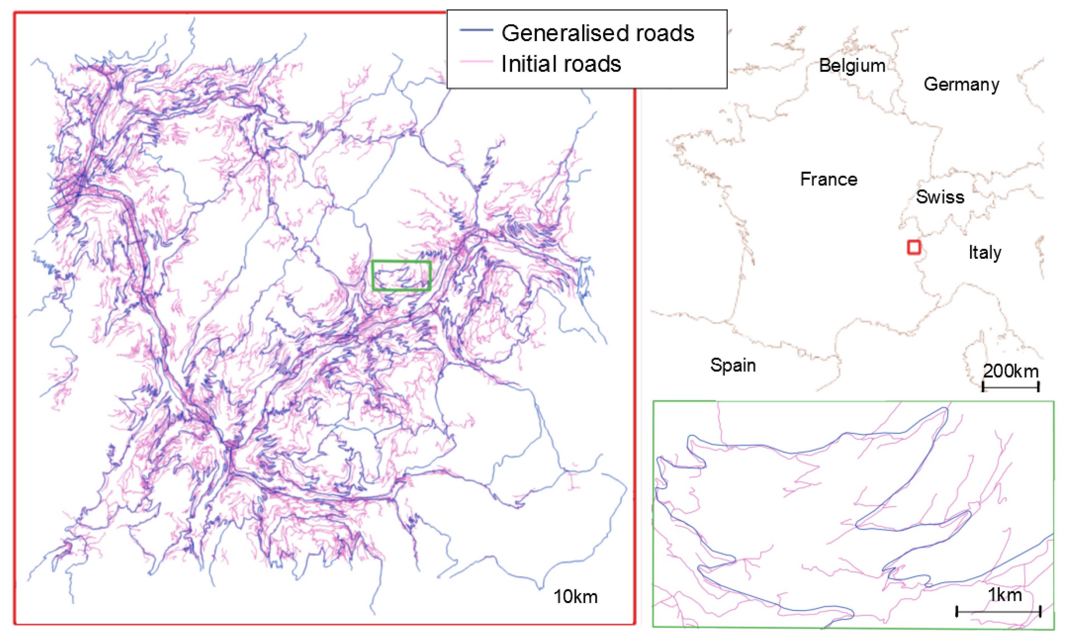
We used two different datasets of roads covering a small part (2155 km2) of the Alps in France (Figure 1). The first one is an extract of the database used to make the topographic maps at the 1:25,000 scale at IGN, the French national mapping agency (NMA), and it contains 30,455 roads for a total length of 5,253,248 km. The second dataset is an extract of the database used to make the 1:250,000 scale map at IGN, it contains 853 roads for a total length of 1,775,205 km. This second dataset represents only important roads and their shape is simplified, smoothed, and often schematised for a better visualisation of the sinuous bends. The goal of this use case was to generate the 1:250,000 scale map from the 1:25,000 scale map.
These datasets are constructed and managed independently, therefore there is no direct link between corresponding roads and the road attributes are not similar.
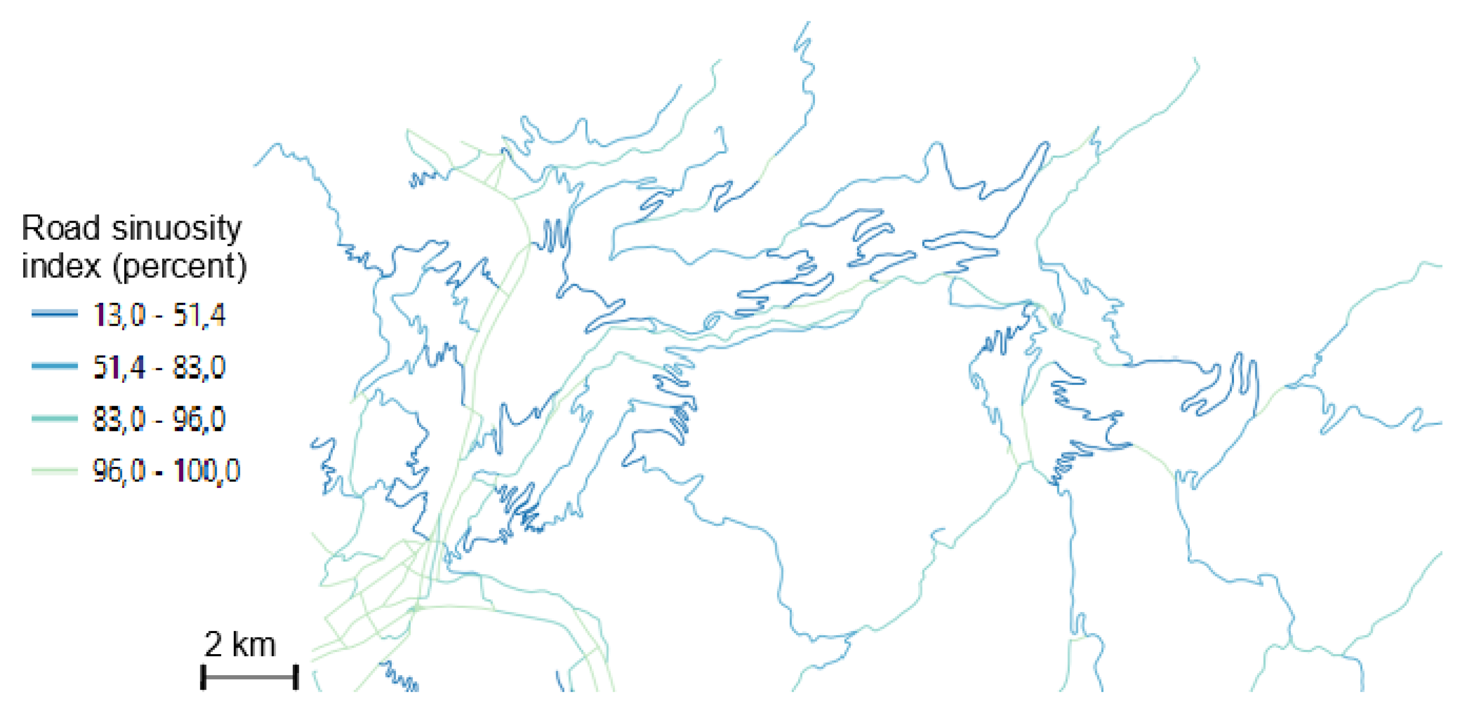
The second dataset was generated from the first one by a generalisation process that combines automated algorithms and manual corrections by cartographers twenty years ago [19], and then manually updated by cartographers. The dataset does not contain only sinuous mountain roads, it contains all the roads of the area, so there were also some urban roads in towns and one highway across the map. We split our dataset in two subgroups according to sinuosity (Figure 2), in order to test different training methods, i.e., to try a training with all types of roads and a training only with sinuous roads, the most difficult to generalise. We chose a simple measure of road sinuosity [7]: for each road polyline, we divided the base length (distance between the first and the last vertices) by the total length of the road. This measure is given as a percentage in Figure 2: the value is close to 100 when the road is straight and close to 0 when it is very sinuous.
As a first step, we do not want, in this paper, to learn both road simplification and selection. In order to identify the roads from the source dataset that were kept in the output dataset, a data matching pre-process between both datasets was necessary. There were very large gaps between the corresponding roads from both datasets (often several hundred meters), so the classical road matching method we used [27] was unsuccessful. As a consequence, we finally decided to manually match the roads that are present in both datasets. As a manual matching would not be a reasonable solution for larger areas, the use of more flexible multi-criteria data matching methods should be investigated [28].
3.2. Mountain Roads Generalisation as a Deep Learning Problem
We aimed to use a convolutional neural network (CNN), as it was successful to generalise buildings [10]. Therefore, in this section, we detail how to represent our problem with images. CNN are networks adapted for image processing tasks, such as image classification, or segmentation. In a segmentation model, the class of each pixel is determined by the model. In our case, each pixel was classified in one of the two classes: generalised road or background.
There are other possible ways to model road generalisation as a deep learning problem, for instance by using graph convolutions [29]. But we think that CNN segmentation is adapted because all the information necessary to draw a generalised version of a road can be included in the image of the road [8]. The usual constraints defined for mountain road generalisation are the following [16]:
- coalescence (there should be no symbol coalescence when the width of the road symbol is large enough for display scale);
- granularity (details of the line that are too small to be visible at display scale should be removed);
- position (the generalised road should be close to the initial road);
- smoothness (the generalised line should be smooth);
- general shape preservation (the generalised road should be similar to the initial road);
- sinuous bends and bend series preservation (the presence of sinuous bends or bend series should be preserved, at the risk of removing some of the bends in a series).
As long as the images used in the CNN depict the road with enough detail to “see” granularity, coalescence, or bends, the CNN should be able to learn the implicit knowledge to transform the road image while satisfying these constraints. Therefore, we had to construct paired images: one should be the input of the model and the other the target, from the vector roads. This process is explained in the following subsection.
3.3. Creating an Adapted Learning Dataset
The vector to raster transformation can generate some errors [30], as rasterization always causes a loss of information compared to vector data. Errors can occur on the area, the perimeter, the shape, the structure, the position and the attributes of the rasterized data, but only errors in shape, structure and position are relevant for us. Increasing the resolution of the raster image can minimize these errors, but a larger image has a consequence on the computation time of CNNs, and does not always improve final results. For instance, the classification results from [31] are better with a 256 × 256 size than with a 512 × 512 size (with a constant scale). Convolutional neural networks are designed to optimally work with squared images with a size which is a power of two (e.g., 128 × 128, 256 × 256, etc.). Consequently we choose 256 × 256 images, which is empirically a good compromise between the resolution of the images and computation time. We can also note that the size of symbols is important to define during rasterization. Symbol size is a classical problem in raster generalisation [32].
Consequently, we decided to generate our 256 × 256 images with red roads on a white background. Using a coloured image, even if only one colour is used for now, allows a further addition of information (e.g., buildings or rivers) without transforming the network architecture for accepting coloured images as input.
We can include some additional information by assigning width symbols relative to road importance. We matched the attribute values defining road importance in both datasets to a width in pixels, and this matching is summarised in Table 1.
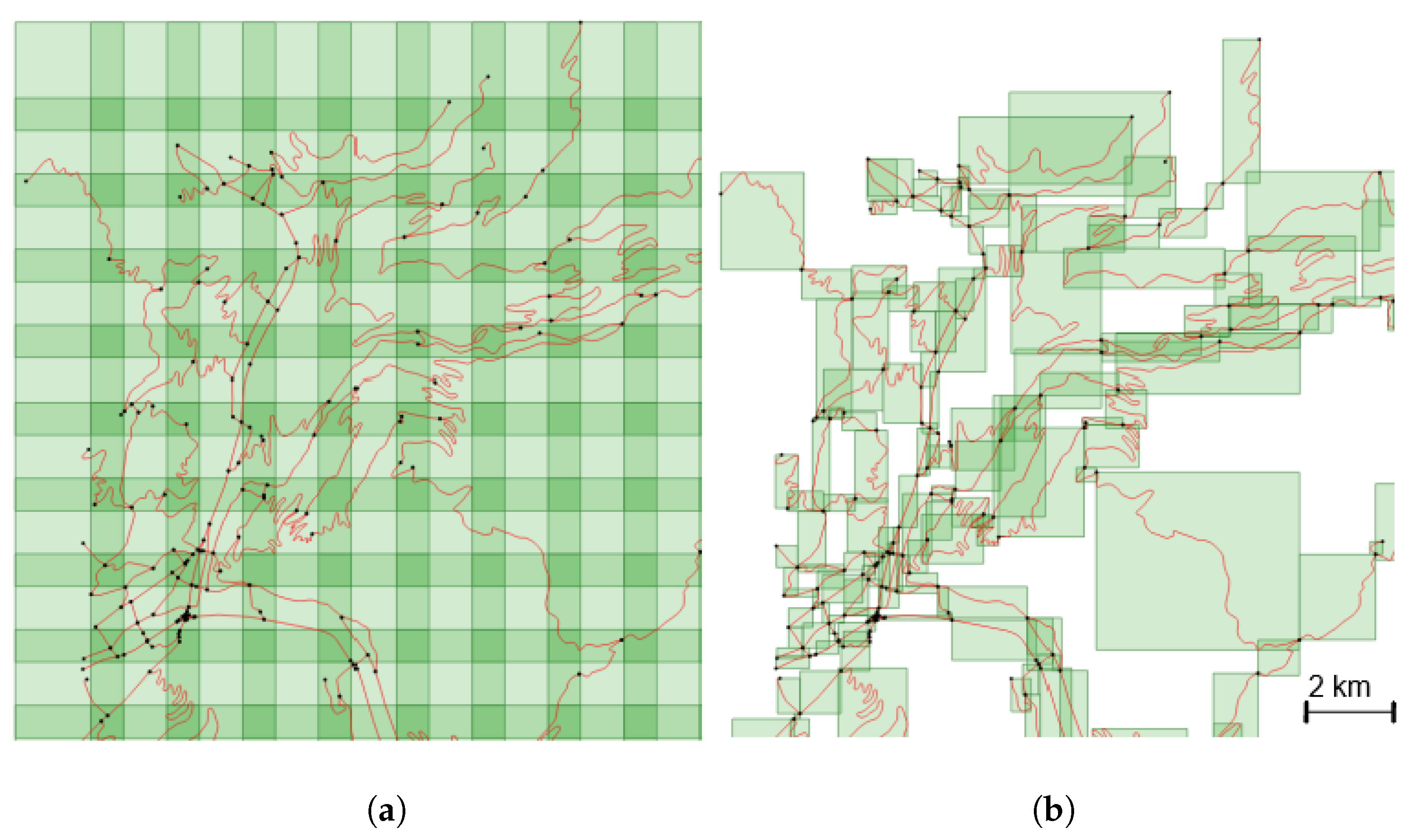
Then, we propose two approaches (illustrated in Figure 3) to create the images by tiling the dataset:
- to slide a fixed-size window over the study area. This method creates images with a fixed scale of the underlying data, but can generate irrelevant (only a very small portion of a road) or empty tiles.
- to overcome the problem of irrelevant tiles, we can use the road objects as a basis to guide tile creation. In this method, the whole geometry of a road is included in the tile, and as roads objects have varying lengths, and geometry extents, this process makes tiles that have different scales.
It should noted that, in the initial database, a new road is collected at each intersection and at each change of attribute (e.g., change in the number of lanes or in the width of the roadway). This is why roads do not always terminate at intersections.
The first method needs two parameters: a window size (or resolution) and an overlapping rate that defines the window displacement over the dataset. The second method does not need any parameter.
The problems raised by both methods are similar to classical problems in data partitioning for map generalisation [33], where there is no perfect solution. There are two important issues to consider here: first the scale of the images should be fixed to help the convolutional network to learn that scale changes from the input image to the output image. Then, there is the classical issue of the best level of analysis for generalisation [34], which is particularly significant when dealing with mountain roads [16]. For instance, working on the level of dataset road objects is arbitrary, as these objects can be very long or very short, and not always homogeneous in terms of shape. Working on road strokes [11] might be a better choice, and/or working on parts of roads that are homogeneous in terms of sinuosity or symbol coalescence [16].
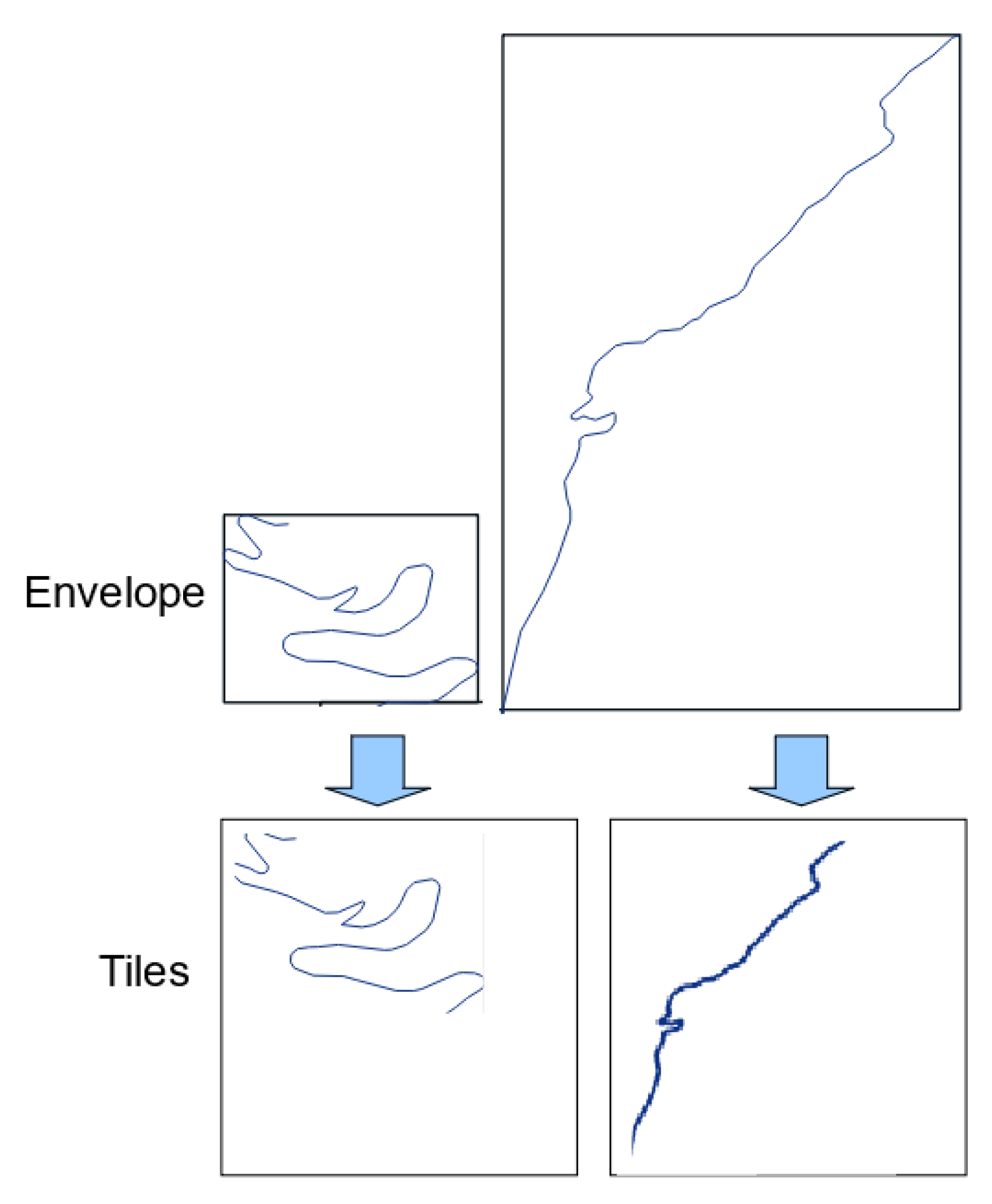
As none of the proposed methods is ideal, we decided to post-process the tiles generated. The first post-process consists in cleaning the tiles that lie at the limit of the use case area, when they do not contain roads from both datasets due to selection edge effects. Regarding the first method with fixed-size tiles, we removed the irrelevant tiles that contain no road or only a very small portion of roads. Then, regarding the second method, we tried to reduce the effect of varying scale by applying a road width fixed with scale (images at smaller scales have thinner road symbols). As shown in Figure 4, when the roads are smaller than the tile, symbol width remains unchanged, and the road width is 1, when the extent of the road is greater than the tile, the reduction ratio is used to choose the width of the roads following Equation (1).
The envelope is the minimum bounding rectangle parallel to the X and Y axes around the road. The length of the envelope is the length of the rectangle side parallel to the X axis, and the width is the length of the rectangle side parallel to the Y axis. The gap is a small blank space that we introduced around the image.
As result of these processes, we obtain around 560 images with the first method and 690 with the second one.
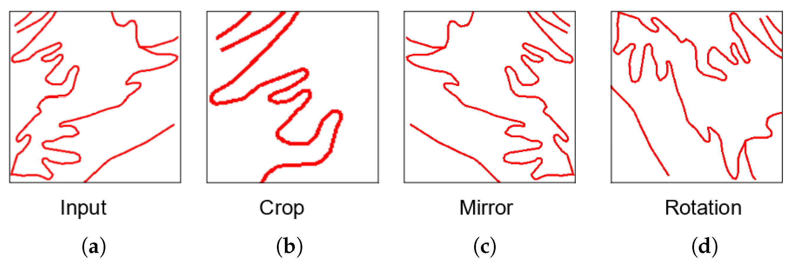
To increase the number of images for training, three common methods exist [35] that generate modified images from existing ones: crop, mirror, and rotation (see e.g., Figure 5).
In our case, using the crop augmentation (cut a part of the image) does not seem to be adapted: on object-based tiles, we lose a part of the context (around the object), and in case of fixed-scale tiles, images of the new dataset do not have a fixed scale. The rotation (90, 180, or 270), and the mirroring (according to a horizontal or a vertical axis) augmentation methods have similar effects on the image and augment the training set with realistic new road images.
It is also possible to augment the number of images by changing the tiling parameters. In the object-based approach, considering smaller objects than initial roads, especially in the case of very long roads, would augment the size of the training dataset. In the fixed-sized method, choosing a smaller window or using a bigger overlap would augment the size of the training dataset. These alternative augmentations were tested and presented in Section 4 to assess their usefulness.
But data augmentation does not solve problems of representativeness and homogeneity because it will augment much more the number of non sinuous roads if they outnumber the sinuous roads in the initial dataset, which is the case in our use case.
3.4. Choice of a Neural Network Architecture
The generalisation problem was modelled as an image segmentation problem with an image as input and a classification of each pixel in two classes (road or background) as output. Many different network architectures exist in the literature to solve this kind of problem [36]. Deep learning networks are neural networks with a deep architecture, i.e., many layers of connected neurons. The goal of these networks is to find a predictor that minimizes the error (loss) function. Convolutional neural networks (CNN) are a specific type of deep neural networks, and are useful in visual recognition and classification tasks because of their ability to process matrix data, such as images, at different scales. These networks are inspired from the human visual system. CNN principles are based on a succession of convolution layers that apply a filter to the image, and pooling layers that reduce the size of an image through downsampling.
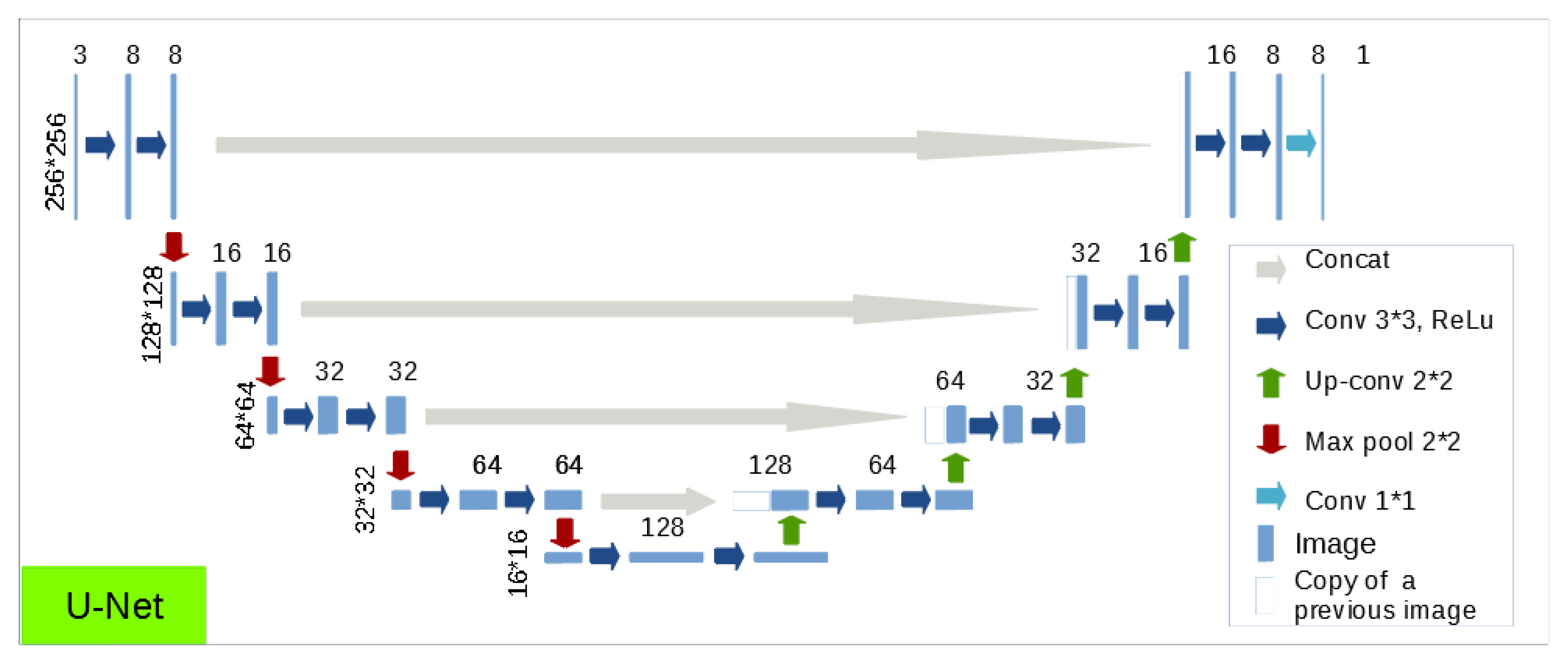
Following the results of the first experiment on map generalisation [10], we choose to test the U-Net architecture [9]. This network was first developed for segmentation of medical images. It consists in a series of convolution and upconvolution layers into a contracting path that follows the typical architecture of a convolutional network and an expansive path (right side) that reconstructs the spatial size of the input [37]. In order to manage border effects, it introduces skip connections (concatenation) which link earlier layers with deeper layers of the network. This network was able to achieve very good segmentation results in different types of applications. Our implementation of this model is presented in Figure 6, the size of each image is presented on the left of the line and the number of channels at the top of the image. It is very similar to the original one except that we used, as input, coloured images of 256 × 256 pixels.
In Figure 6, the initial image is the element of size 256 × 256 in three channels at the top left; at the top right you can see the output, which is a black and white (one channel) image of the same size. Each arrow represents a neural layer. First in dark blue there are convolution layers with a filter of size 3 × 3. Such layers are always followed by an activation function called rectified linear unit (ReLU). In red, there is the “max pooling” layer which allows reduction of the size of the image: it keeps only the maximum value for each block of size 2 × 2. In green, the up-convolution layers augment the size of the image and reduce the number of channels. In grey, at each level a concatenation layer do the skip connection. Finally, we provide a fully connected layer (light blue) to obtain a segmentation map.
3.5. Evaluation and Loss
In this article we mention two kinds of evaluation: first the auto-evaluation of the network that allows the convergence of the model at each epoch, this is the quantitative value of the loss function; second, the final evaluation of result that assesses if the model succeeds to learn the task. The following paragraph presents existing measures that exist for both evaluations in segmentation.
There are many ways to evaluate the result of a segmentation in artificial intelligence, most of them take into account the contingency of a class pixel between the predicted classes and ground truth. All segmentation evaluation methods measure how different the pixels are in ground truth and prediction. Nevertheless the choice of the measure is important, because all pixels do not have the same importance in evaluation. For example, in a building generalisation task [10], only the pixels around the building border are decisive. The authors of [38] compare different evaluation methods for segmentation problems. The intersection over union method (IOU) is common for the evaluation of segmentations with two classes, as it represents the intersection over the union of pixels in road class (in our use case) in both prediction and ground truth. As roads are depicted by few pixels in each image, a measure that is not sensitive to unbalanced classes would be useful, such as the Dice coefficient which represents the double of the intersection over the sum of the count of pixels in road class in both prediction and ground truth.
These two measures can be relevant for our segmentation problem and we tested both in our experiments for the evaluation of final results. Nevertheless, both measures are not really adapted to evaluate a good generalisation result as the output of the segmentation: a good segmentation can suffer local problems that reveal a very bad cartographic result [26]. In our case, the segmentation tends to create loops in sinuous bends rather than just enlarging bend (see the results in the following section). This is not a big segmentation error because only a few pixels were misclassified, but it is clearly an important cartographic mistake. Consequently, we carried out a complementary evaluation with a visual rating of the results.
Regarding the loss function that acts as an auto-evaluation of the model, the same remarks apply, as the unbalanced nature of both our input and output images is not well conveyed by the default loss functions that we used in this model. The conception of an adapted loss for cartography and generalisation is a perspective raised by our work.
4. Results and Evaluation
4.1. Implementation
We conducted our experiment using Python 3 with the Keras library [39]. The code was implemented in the Google Colaboratory platform with the available graphic processing unit (GPU) for standard licences. Our code and image data will be made available in future weeks as part of the DeepMapGen open platform https://github.com/umrlastig/DeepMapGen. The code to generate the images from the vector dataset was part of the CartAGen open source generalisation platform https://github.com/IGNF/CartAGen, developed at IGN [40].
In deep learning, the data is separated in three sets. The training set is the set of images used to train the model. At each iteration (or epoch), additional data, not from the training set, called the test set, are used to assess and adjust the model. Finally, the evaluation set is not used in the training process and serves in the evaluation of the trained model on new images. We chose to evaluate our model on 4% of our dataset. This is unusually low but our initial dataset was small (see Section 3.1) and we wanted to keep it large enough for an effective training; however, this ratio allows for the representation of most situations. We randomly separated our dataset into a training and an evaluation set, and we added the constraint that evaluation tiles should not be spatial neighbours. Then, the training data was further randomly separated into the real training set and the test set. Consequently, 92% of our images were used for training.
In this experimentation, we had to choose a loss function for the model. The loss function indicates the error of the model and the network tries to minimize this function. U-Net typically are implemented with a binary cross entropy loss (BCE). This loss was calculated considering the probability map output for each pixel being a road.
where is the label (1 for roads and 0 for not road) of the pixel i, and the predicted probability of the pixel to have this label.
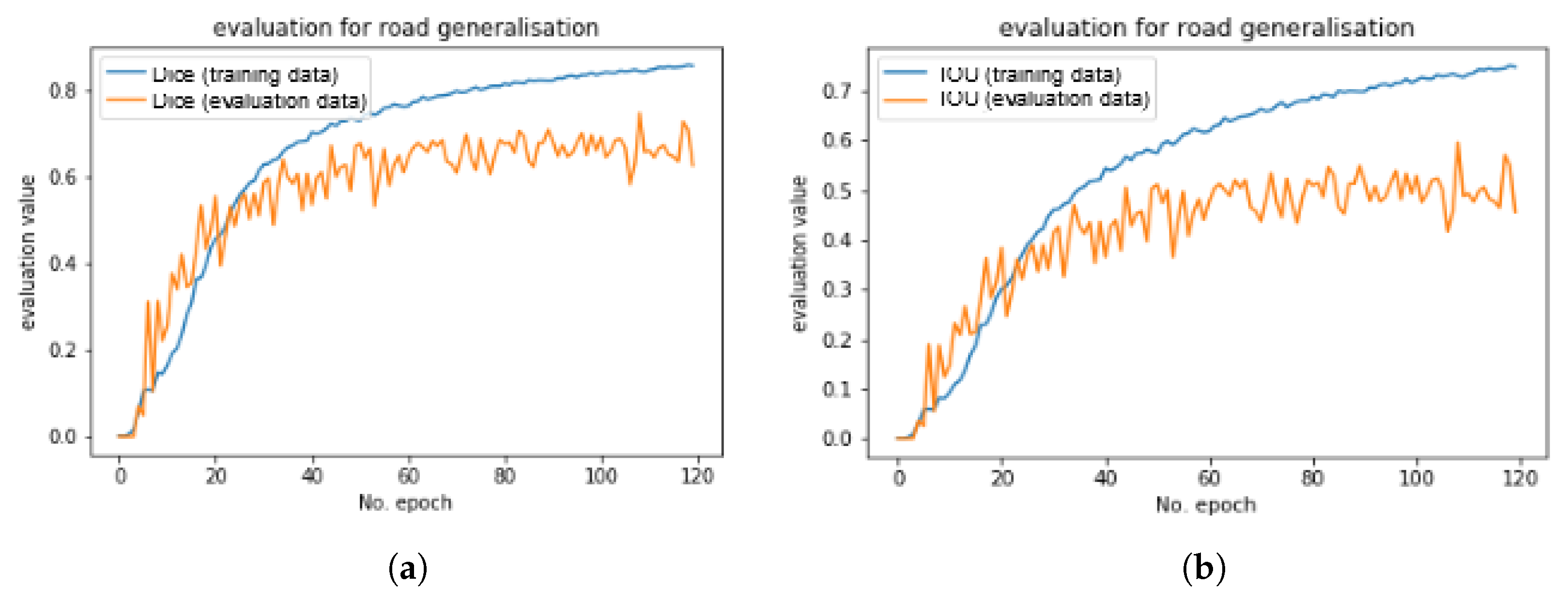
We also needed to set an optimized number of epochs. An epoch is one learning cycle that takes into account all training images. Figure 7 presents the evolution of the network loss on the training set and on the evaluation set over epochs. The number of epochs should be relative to the size of the training set to avoid over-fitting. As the size of the training dataset is small, this number of epochs should be kept small.
To determine the most suitable moment to stop the network (i.e., the number of epochs), we could save the model at checkpoints every 20 epochs, and observe the result for this current model. The evolution of the loss presented in Figure 7 is another way to assess the optimal number of epochs. To obtain our best results, we chose to stop the training at 120 epochs, despite a quick stagnation of quantitative quality after epoch 50, because there is a progression of the visual quality of the predicted images, and the predicted images generally stop improving beyond this threshold.
The loss curves, and especially the fact that the loss is not strictly decreasing, indicate that the loss function could be sub-optimal, as it is not consistent with the visual improvement of the prediction; therefore, we tested several other loss functions that were available in the Keras library, and especially the mean square error that is another common segmentation loss; however, these functions were not adapted either as they measure the global quality of pixel classification, and results with these other loss functions were worse than with the binary cross entropy loss. The research for an adapted loss is an important perspective of this work.
Another important point to note is the difference between loss values for training and validation images. The further these curves are the more over-fitting there is. In this case, the difference was around 10 percent whereas in case of smaller datasets (e.g., when using the object-based tiling approach, or with a lower overlapping rate between tiles) we have very different loss values between training and evaluation. That again shows the interest of choosing an optimised image construction method.
4.2. Results
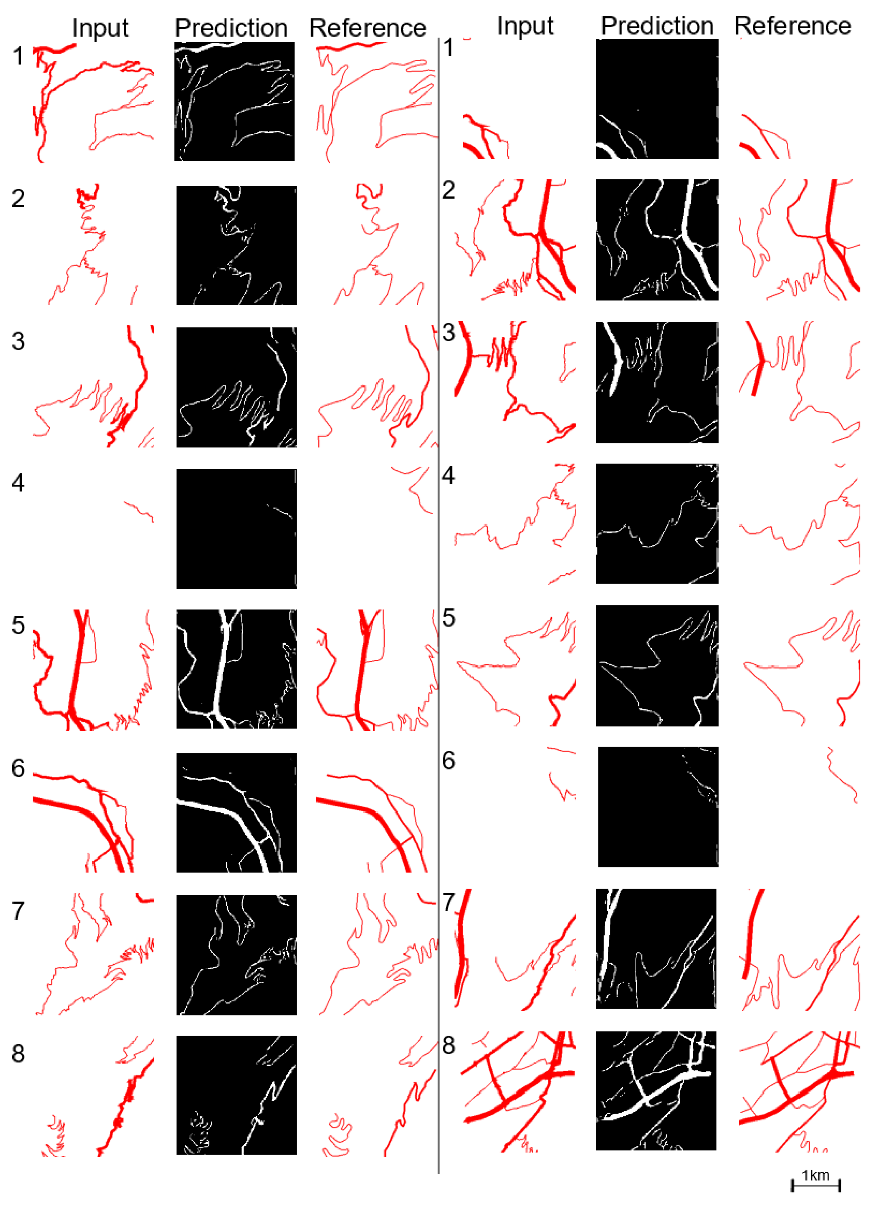
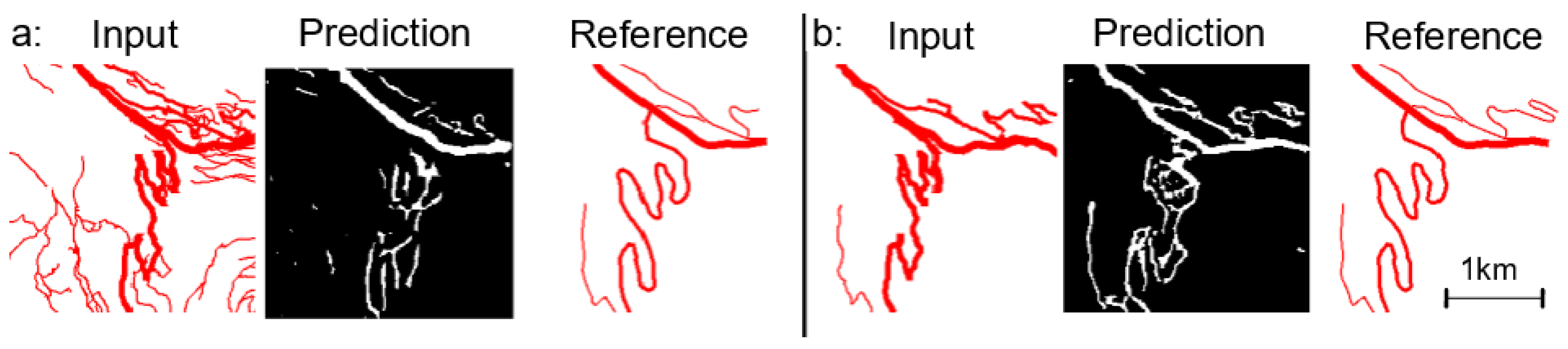
In this section we present some results obtained with the U-Net segmentation of mountain road images. Our model reaches a segmentation accuracy on evaluation (and train) dataset around 60 percent (80 percent) according to the Dice measure and 50 percent (70 percent) according to the IOU measure. Moreover, the error measured by the loss function decreases under 0.10 (0.03). Figure 8 shows some of the results obtained on the images of the validation set. The figure shows the initial image on the left, the predicted image in the middle (black and white), and the ground truth image on the right. In most of the images, the road shape is recognizable, and is very similar to the generalised image. It is also often smoother than the initial image, even if it is sometimes less smooth than the generalised one. Bends are enlarged in most sinuous bend series, but the enlargement is sometimes not correct, which can lead to loops or U-shaped bends. In some cases, in the ground truth, roads are displaced between initial and generalised image to avoid overlaps with other objects (river or rail line). As such data are not visible in our images, the model is unable to learn when such displacement should occur and fails in these images. Moreover, our method does not guarantee the network connectivity inside each tile, and often some roads are disconnected in the predicted image. This is a serious drawback that is discussed later in Section 5. Sometimes, there are roads in the generalised image that do not exist in the initial data, and these roads are obviously not generated by the model: sometimes, e.g., the fourth image on the left column, the model does not generate any additional road at all; in other cases, e.g., the sixth image of the second column, the model can add road segments that are not in initial data, but they do not really correspond to the ground truth additional roads. Finally the third image of the right column shows the generation of a new very small section of road that follows the right edge of the image that does not exist either in the initial image or in the generalised one.
Figure 9 shows the evaluation scores of the model with both evaluation methods: Dice and intersection over union (IOU). They were computed at each epoch on the training set and the evaluation set (that is not used to train the model).
The evaluation score is unstable between consecutive epochs, so the value at the end of the process is less relevant than the last epochs’ mean evaluation (e.g., the mean of the last 10 epochs). The two evaluation measures return quite poor quantitative results. As explained in Section 3.5, the comparison of pixels with a reference is not adapted to evaluate generalisation; it explains the low score of both measures. We also observe that measures are not always coherent with our quality perception but it generally provides a good indicator.
The presented results are obtained using some parameters to configure the model. The calibration of the parameters is described in the following subsection. The parameters used to derive the tiles are the following:
- tile size is 2.5 km and a pixel represent 10 m;
- overlapping rate between tiles is 60 percent;
- road width represents importance level;
- the included roads are only the roads that matched during the pre-process matching.
All these parameters could influence the result. We study the impact of these parameters in Section 4.3.
4.3. Training Dataset Parameters
In this section, we evaluate the proposed method for creating the training dataset. Table 2 summarizes the results of this evaluation.
4.3.1. Is Data Matching Pre-Process Useful?
First, we compare the results of segmentation when the initial images contain all the roads of the initial dataset, even the roads that are removed in the selection process, with our standard results without those roads that are not matched with generalised roads.
We can see in Figure 10 that removing the unselected roads from the initial image seems to be a better solution but the results in both cases are quite unsatisfactory for this road. We can note that the network did learn to remove the unimportant roads, but did not do it properly (some road parts remain, and one important road on top is partially erased). Road network selection is based on global metrics in the network [12], so we do not expect that a CNN could learn how to select the important roads in a very small extract of the network.
4.3.2. Comparison of Tiling Methods
In this subsection we try to compare the two proposed approaches for tile generation (fixed-scale and object-based).
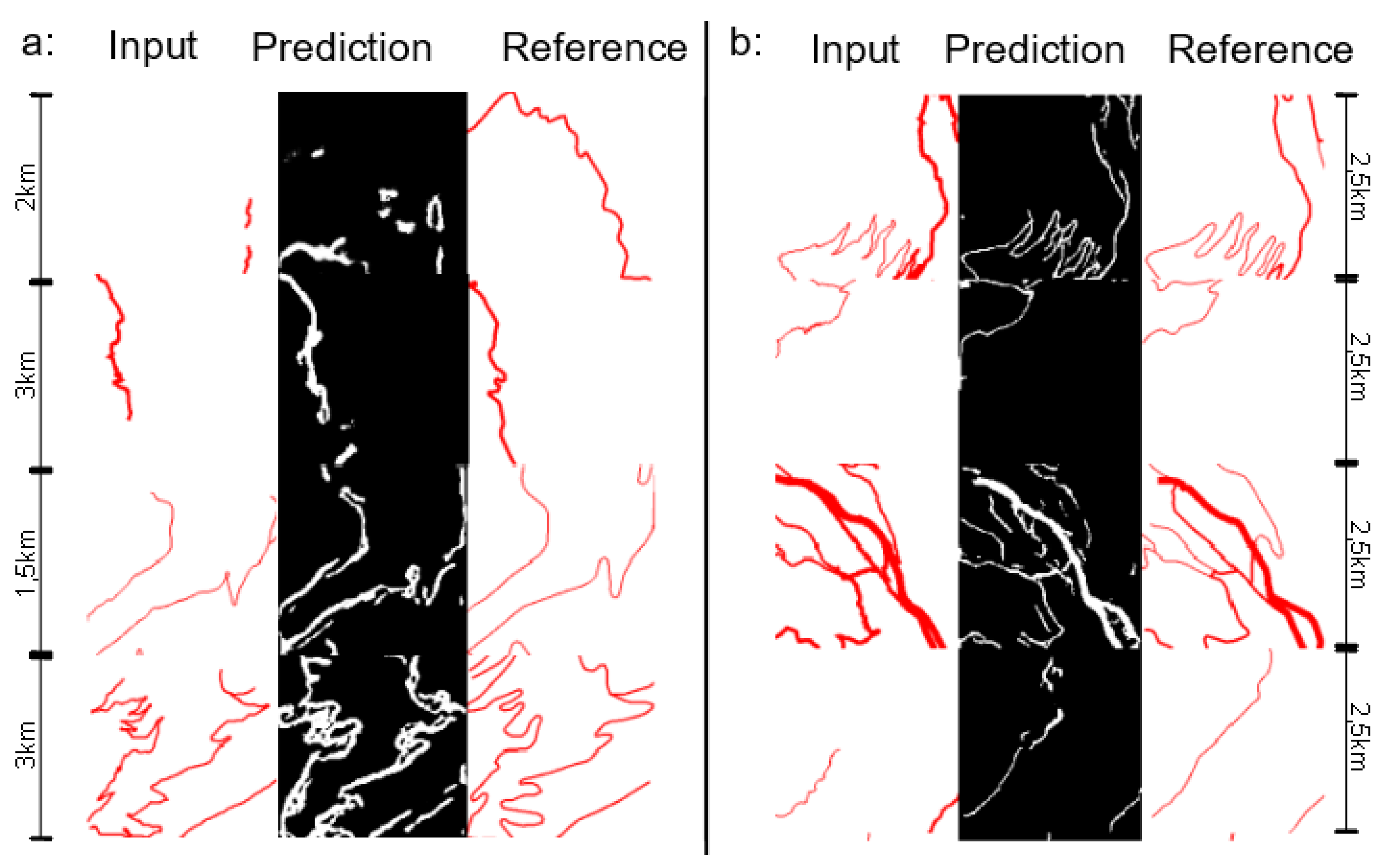
We observe in Figure 11 that the fixed-scale tiling approach gives better results than the object-based approach. The object-based approach seems to systematically create loops in bends and enlarge the road symbols too much (it is probably due to its varying scale). This difference could be due to the construction and filtering method. It should be noted that training on the non-filtered dataset gave poor results with both tiling methods.
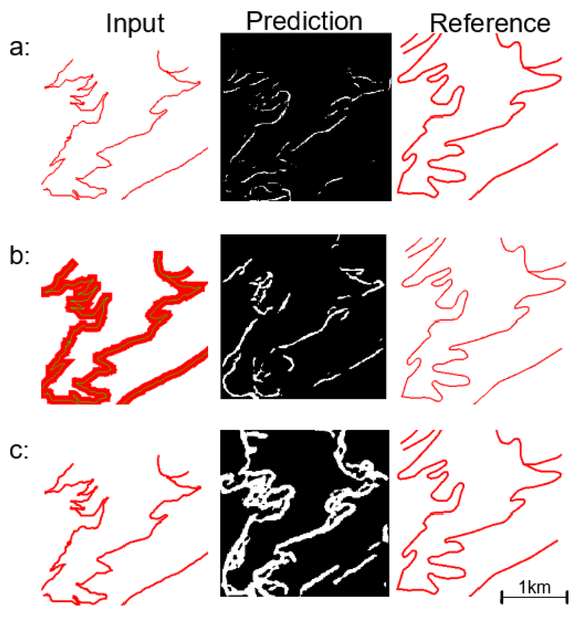
We suppose that the “loop” problem is caused by the coalescence in the initial image, which prevents “seeing” the initial shape of the line. This is why a mixed representation of roads in input images was tried: the shape of the line is displayed in green with a width of 1 pixel, overlayed on top of the larger red symbol that coalesces. Figure 12 presents a comparison of results given by this mixed representation with the object-based method. The mixed method is compared to an image where symbol width is left unchanged, and to an image where symbol width is exaggerated to convey the scale reduction due the size of the road. It shows that the shape readability improves thanks to the green thin lines, and it does reduce the “loop” effect but the results remain unsatisfactory. This handling of bend series with a heavy coalescence needs further research.
4.3.3. Calibration of the Fixed-Scale Tiling Approach
As explained in Section 3.3, the main problem of this approach is to randomly cut roads, degrading context (i.e., the global shape of the road). So a calibration that preserves the context as much as possible should give better results. The size of the tiles is a parameter that impacts two characteristics: the context and the number of images. We measured this parameter in terms of ground size represented by a 256 × 256 pixel image. It is not relevant to choose a size under 1 km (not enough context). As a result, all pixels are classified as “not road”. Conversely, over 5 km, the study zone covered was too small to have enough images (less than 150). We observe that sizes between 2.5 and 3 km are the more relevant for our tasks.
Figure 13 presents some results of an experiment about tiling size we carried out to confirm our visual observations. We can see that smoothing is not well learned when the model is trained with large areas (5 × 5 km). The coalescence of small bends that increases with size gives bad results, so the size of tiles should remain small to minimize symbol coalescence in input images.
The last parameter of the fixed-size tiling approach is the overlapping ratio between tiles. This parameter allows for the augmentation of the number of tiles. Experiment with 40%, 50%, and 60% values show a good progress in both qualitative and quantitative evaluation when overlap increases. Moreover this overlap allows us to have some redundancy as roads appear in several images. We believe that we could merge these classification results in different images to improve the generalisation of one road.
4.3.4. Importance of Road Sinuosity
In this section, we study the impact of the imbalance between straight roads that are easy to generalise, and more rare sinuous roads that are complex to generalise. There are several questions related to this imbalance: is the network able to generalise areas with mostly straight roads, or areas with only very sinuous roads? Would the model work better on sinuous roads if it was trained only on tiles containing very sinuous roads? When separating data according to the sinuosity of roads, it significantly reduces the number of images but increases the homogeneity. We propose two ways to separate sinuous from non sinuous roads, depending on the tiling method. For the object-based approach, the criterion is simply the sinuosity of the road the tile is centred on; for the fixed-sized approach, we use the mean sinuosity of the roads inside the tile, weighted by the length of the road. For this experiment, we measured the sinuosity by dividing the base length by the length of the line [7] and we used a threshold of 0.7. The results clearly suffered from the lack of images with sinuous roads, but they are promising for the object-based approach. It would be interesting to test this approach with much more images of sinuous roads.
4.3.5. Summary
In this subsection we present a summary to show what seems to be the best approach and parameters to derive the training dataset. Table 2 contains the evaluation of each test in terms of Dice value, IOU value, and qualitative comparison with a reference situation (REF). The values of the table are the following: if the predicted images are visually better than the reference prediction, the visual rank is noted (+), if the predicted images are worse than the reference prediction, the visual rank is noted (−), and if the predicted images are similar to the reference prediction, the visual rank is noted (=). The number of images is also given for information.
The reference prediction for fixed-size tiling approaches is produced by sliding from the top left corner of the zone a 2.5 km square tile with an overlap of 40 percent over the roads, with a symbol width representing the importance. For object-based approaches, each image represents the roads in the extent area of one generalized road (with the initial segmentation of road features). And the road width represents the transformation (resizing) of the image.
4.4. Usefulness of Data Enrichment and Filtering
The filtering is clearly necessary, as the use of (almost) blank images in the training process makes a stable loss and bad learning. Another possible filtering process is to exclude tiles that represent complex not mountain situations (such as highway interchange or roundabouts). Our experiments show that this filtering is not useful, as results are similar.
In deep learning, the size of the dataset is often an important success criterion. When the available dataset is limited, data augmentation allows us to improve results. We discussed several methods to augment the training dataset in Section 3.3, and here we present an analysis of the impact of such methods on the results of the segmentation model. The following augmentation processes were tested on the training dataset:
- Randomly horizontally and vertically cropping 10% for all images;
- Randomly horizontally and vertically cropping 20% for all images;
- Rotate half of the images in a random way (90, 180, or 270 degrees);
- Rotate all the images in a random way (90, 180, or 270 degrees);
- Rotate all images with the three angles (90, 180, and 270 degrees).
First, the dataset produced by the object-based method seems to be the most affected by the data number limitation. We present in Table 3 the effect of augmentation.
In the object-based approach, the small sized crop transformation seems to have a positive impact on the results, it augments the information without hiding the context too much. In all cases, the variability of the evaluation value seems to increase. The rotation seems to augment the quantitative evaluation value, so the prediction is closer to the reference. But it seems to introduce a white spot noise in the images when we visually evaluate the results.
Then, in the case of the fixed-size tiling approach, the crop augmentations are not a good option because it distorts the images and reduces the context around the road (Table 4). The augmentation by rotation are relevant but do not improve the result. It shows that the problem of our dataset is less the total quantity of images than the diversity of situations visible in images (we lack sinuous roads).
Although all experiments show that data augmentation improves the quantitative evaluation, it is worth noting that in this use case, increasing the number of images is not always relevant, and seems to increase variability between the epochs. Increasing the number of images by changing the tiling method could be preferable.
5. Discussion
Even if we did not expect predicted results that are as good as or better than the reference, the results remain really far from this reference generalization for now. In this section we discuss the remaining errors and try to explain their causes. The primary problem is what we called the “loop” problem, illustrated in Figure 11, where road segments are added at the base of the bend, closing the line and forming a loop. The problem mainly occurs when the model is trained with data generated with the object-based approach. We could note two possible causes of this problem: the lack of images representing very sinuous road and the lack of readability or resolution of these images.
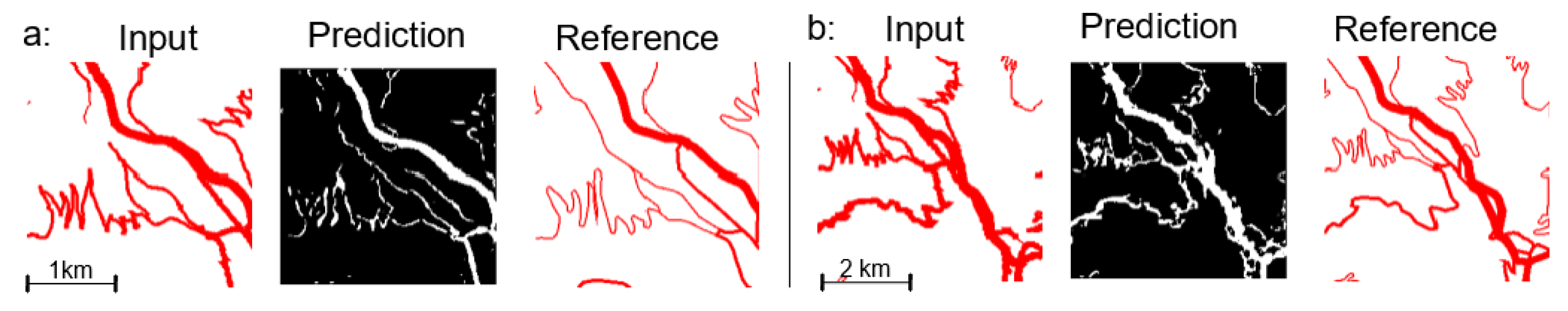
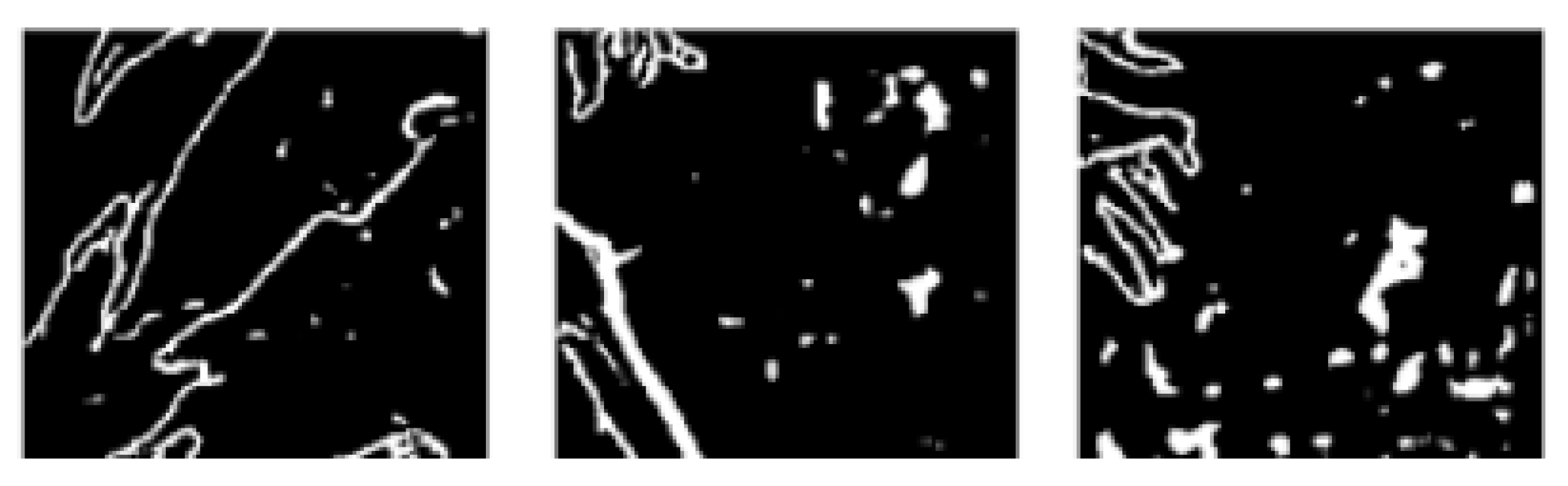
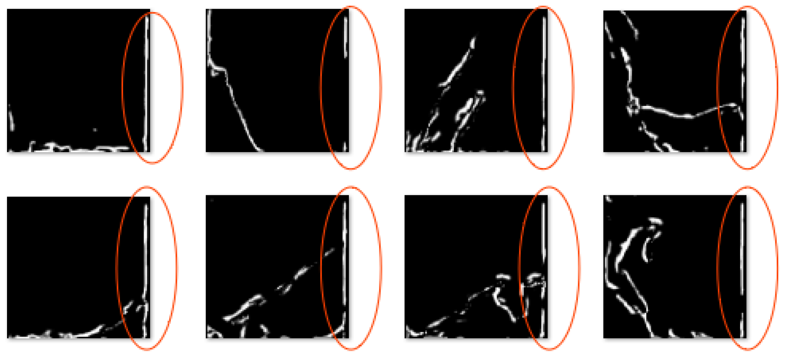
The second problem is the noise appearance. It is rare but significant. We observe this problem in all our experiments when the number of epochs is rather small (under 70), when the number of images for training is small (under 150), or when the real size represented by the tile is extremely large (above 5 km2). We observe two kinds of noise: white spots (Figure 14) and the creation of a fictitious road (Figure 15).
We can observe that the white spots on all these images are not regular and always appear in areas where there is no road. This noise can easily be post-processed using a morphological operation.
In the case of fictitious additional roads (Figure 15), the problem always occurs on the same side in all images of the evaluation set, but the shape of the added roads is not always the same.
The third problem is the visible connectivity alteration on all our images. It consists of the appearance of a few black pixels in the middle of some roads, that do not much alter the quantitative evaluation but clearly degrade the road legibility. This problem is less present if we augment the number of epochs, but still occurs. It could not be reduced with a morphological operator applied on the output image during post-processing, without damaging the rest of the road shape. Then, the only post-process that could re-establish connectivity would be to convert the roads back into vectors and use connectivity checking techniques from road network generalisation [12]. On the contrary, we imagine that it is possible to produce images without this problem using an architecture that learns the characteristics of a road, including its connectivity, such as a generative adversarial network (GAN). GANs include a generator that produces an image (generally a U-Net such as the one used here), and a discriminator that learns to discriminate realistic and continuous roads from disconnected outputs such as the ones obtained here. We will investigate in this direction in future research.
Our work also experienced limitations that are not errors:
- the evaluation measure, and associated loss function should be improved;
- our dataset has a limited size and it does not contain enough examples of very narrow and sinuous bend series;
- we also faced computation time and memory limitations.
Our current examples do not even reach the level of quality of the previous research on buildings [10]. As explained previously in the paper, the scale in the tile generation process is an important problem. It seems that our training images are much more complex than the training images for building generalisation, which only contain a single building or a building part. Our current images contain too many details that are represented by only a few (fuzzy and crowded) pixels. This complexity in our input images has at least three consequences: (1) we need more examples to train the model; (2) we need larger images or images with a better resolution; (3) the network needs to be much deeper than our current setting if we were to use images of such a complexity. If we want to maintain our current decision to including so many road segments in a single image, we should at least try to increase the image dimensions. Furthermore, in order to learn to displace the roads for example, we only need to know that there is other map objects in close proximity, we do not need a much larger context. We were limited in our experiments by the computational issues, and the time it takes to extend our initial dataset by performing a long manual data matching pre-process. Consequently we did not test these improvements yet.
6. Conclusions and Future Work
Our work has shown the ability of deep learning methods to achieve generalisation tasks from images derived from vector data, as a segmentation task. Therefore, it can be perceived as an extension of [10] on a more complex problem due to the complexity of mountain roads generalisation, and the large scale gap (1:25,000 to 1:250,000). The model we proposed correctly achieved smoothing, enlargement, and caricature operations in most of the cases, even if these cases are the simpler ones, i.e., the ones with few coalescent symbols. The proposed segmentation model does not produce better results than the reference (or even close), but it shows that most of the knowledge behind generalisation can be captured by a neural network.
In order to improve the results when road displacement is required, we plan to add other geographic features in our images. As this displacement is often caused by the overlap with the symbols of a nearby river or railway, adding this information in the image should improve our results. We might also be able to generalise these rivers and railways in the same time.
Furthermore, we showed the interest of several propositions in processing the training dataset, but some other propositions can be tested. For instance, the selection process could be integrated, and other scales and datasets could be used.
One of our limitations is the evaluation and the loss function used in the model. Our evaluation method mixing quantitative and qualitative, which provides a good idea of generalisation quality; however, an automated measure integrated in the neural network is preferable. Further work should focus on what a good generalised image is in terms of pixel classification. More generally how could we translate map readability and shape preservation, and more generally the principles of map generalisation evaluation into a loss function. Research about the evaluation of raster evaluation could be extended to deal with deep learning results. For example, the clutter measures could be useful to evaluate the quality of the deep learning output [41,42]. The list of good generalisation criteria could also be formalised as constraints on pixels and groups of pixels, and their satisfaction could be measured. For further work, the quality of the generalization results should be evaluated through some user tests.
Another perspective is to investigate other network architectures for road generalization. The GANs (Generative Adversarial Networks) are frequently used in image generation. Despite not being superior to U-Nets for building generalisation [10], it has great potential to solve most of the limitations of the U-Net predictions we achieved. GANs were used to transfer style in multi-scale maps [23,43], which is a problem quite similar to map generalisation. Our first experiments with GANs were not successful, and are not presented in this paper, but we plan to keep on testing how GANs can generate generalised images.
Finally, the post-process and integration of predicted road into a final map remains an important problem. The raster to vector transformation has to be investigated but also how we can merge the results of different tiles that contain the same roads.
Author Contributions
Conceptualization, Azelle Courtial, Achraf El Ayedi, and Guillaume Touya; data curation, Azelle Courtial, Achraf El Ayedi, and Guillaume Touya; funding acquisition, Guillaume Touya; methodology, Azelle Courtial, Achraf El Ayedi, and Guillaume Touya; project administration, Guillaume Touya; software, Azelle Courtial, Achraf El Ayedi, and Guillaume Touya; supervision, Guillaume Touya and Xiang Zhang; validation, Azelle Courtial, Guillaume Touya, and Xiang Zhang; visualization, Azelle Courtial; writing—original draft, Azelle Courtial; writing—review and editing, Guillaume Touya and Xiang Zhang. All authors have read and agreed to the published version of the manuscript.
Funding
This research received no external funding.
Conflicts of Interest
The authors declare no conflict of interest.
References
- Stanislawski, L.V.; Buttenfield, B.P.; Bereuter, P.; Savino, S.; Brewer, C.A. Generalisation Operators. In Abstracting Geographic Information in a Data Rich World; Burghardt, D., Duchêne, C., Mackaness, W., Eds.; Lecture Notes in Geoinformation and Cartography; Springer International Publishing: Cham, Switzerland, 2014; pp. 157–195. [Google Scholar] [CrossRef]
- Duchêne, C.; Baella, B.; Brewer, C.A.; Burghardt, D.; Buttenfield, B.P.; Gaffuri, J.; Käuferle, D.; Lecordix, F.; Maugeais, E.; Nijhuis, R.; et al. Generalisation in Practice Within National Mapping Agencies. In Abstracting Geographic Information in a Data Rich World; Burghardt, D., Duchêne, C., Mackaness, W., Eds.; Lecture Notes in Geoinformation and Cartography; Springer International Publishing: Cham, Switzerland, 2014; pp. 329–391. [Google Scholar] [CrossRef]
- Regnauld, N.; Touya, G.; Gould, N.; Foerster, T. Process Modelling, Web Services and Geoprocessing. In Abstracting Geographic Information in a Data Rich World; Burghardt, D., Duchêne, C., Mackaness, W., Eds.; Springer: Berlin/Heidelberg, Germany, 2014; pp. 198–225. [Google Scholar]
- Weibel, R.; Keller, S.; Reichenbacher, T. Overcoming the knowledge acquisition bottleneck in map generalization: The role of interactive systems and computational intelligence. In Spatial Information Theory A Theoretical Basis for GIS; Frank, A.U., Kuhn, W., Eds.; Lecture Notes in Computer Science; Springer: Berlin/Heidelberg, Germny, 1995; Volume 988, pp. 139–156. [Google Scholar] [CrossRef]
- Sester, M. Kwoledge acquisition for automatic interpretation of spatial data. Int. J. Geograph. Inf. Sci. 2000, 14, 1–24. [Google Scholar] [CrossRef]
- Kilpelainen, T. Knowledge Acquisition for Generalization Rules. Cartogr. Geogr. Inf. Sci. 2000, 27, 41–50. [Google Scholar] [CrossRef]
- Mustière, S.; Zucker, J.D.; Saitta, L. Abstraction-Based Machine Learning Approach To Cartographic Generalisation. In Proceedings of the 9th International Symposium on Spatial Data Handling; IGU: Beijing, China, 2000; Volume 1a, pp. 50–63. [Google Scholar]
- Touya, G.; Zhang, X.; Lokhat, I. Is deep learning the new agent for map generalization? Int. J. Cartogr. 2019, 5, 142–157. [Google Scholar] [CrossRef] [Green Version]
- Ronneberger, O.; Fischer, P.; Brox, T. U-Net: Convolutional Networks for Biomedical Image Segmentation. In Proceedings of the International Conference on Medical Image Computing and Computer-Assisted Intervention, Munich, Germany, 5–9 October 2015; Volume abs/1505.04597, pp. 234–241. [Google Scholar]
- Feng, Y.; Thiemann, F.; Sester, M. Learning cartographic building generalization with deep convolutional neural networks. ISPRS J. Geo-Inf. 2019, 8, 258. [Google Scholar] [CrossRef] [Green Version]
- Robert, C.T.; Dianne, E.R. The ‘Good Continuation’ Principle of Perceptual Organization applied to the Generalization of Road Networks. In Proceedings of the ICA Proceedings, Ottawa, ON, Canada, 14–21 August 1999. [Google Scholar]
- Touya, G. A Road Network Selection Process Based on Data Enrichment and Structure Detection. Trans. GIS 2010, 14, 595–614. [Google Scholar] [CrossRef] [Green Version]
- Benz, S.; Weibel, R. Road network selection using an extended stroke-mesh combination algorithm. In Proceedings of the 16th ICA Workshop on Generalisation and Multiple Representation, Dresden, Germany, 23–24 August 2013. [Google Scholar]
- Visvalingam, M.; Williamon, P.J. Simplification and Generalization of Large Scale Data for Roads: A Comparison of Two Filtring Algorithms. Cartogr. Geogr. Inf. Syst. 1995, 22, 264–275. [Google Scholar] [CrossRef] [Green Version]
- Lecordix, F.; Plazanet, C.; Lagrange, J.P. A Platform for Research in Generalization: Application to Caricature. GeoInformatica 1997, 1, 161–182. [Google Scholar] [CrossRef]
- Duchêne, C. Individual Road Generalisation in the 1997–2000 AGENT European Project; Technical Report; IGN, COGIT Lab: Saint-Mandé, France, 2014. [Google Scholar]
- Bader, M.; Barrault, M. Cartographic Displacement in Generalization: Introducing Elastic Beams. In Proceedings of the 4th ICA Workshop on Progress in Automated Map Generalisation, Beijing, China, 2–4 August 2001. [Google Scholar]
- Sester, M. Optimization approaches for generalization and data abstraction. Int. J. Geogr. Inf. Sci. 2005, 19, 871–897. [Google Scholar] [CrossRef]
- Mustiere, S. GALBE: Adaptative generalization. The need for an adaptative process for automated generalisation an exemple on roads. In Proceedings of the 1st GIS PlaNet Conference, Lisbon, Portugal, 7–11 September 1998. [Google Scholar]
- Zhou, Q.; Li, Z. A comparative study of various strategies to concatenate road segments into strokes for map generalization. Int. J. Geogr. Inf. Sci. 2012, 26, 691–715. [Google Scholar] [CrossRef]
- García-Balboa, J.L.; Ariza-López, F.J. Generalization-oriented road line classification by means of an artificial neural network. Geoinformatica 2008, 12, 289–312. [Google Scholar] [CrossRef]
- Zhou, Q.; Li, Z. A comparative study of various supervised learning approaches to selective omission in a road network. Cartogr. J. 2016, 54, 254–264. [Google Scholar] [CrossRef]
- Kang, Y.; Gao, S.; Roth, R. Transferring Multiscale Map Style Using Generative Adversarial Network. Int. J. Cartogr. 2019, 5, 115–141. [Google Scholar] [CrossRef]
- Mackaness, W.A.; Ruas, A. Chapter 5—Evaluation in the Map Generalisation Process. In Generalisation of Geographic Information; Mackaness, W.A., Ruas, A., Sarjakoski, L.T., Eds.; International Cartographic Association, Elsevier Science B.V.: Amsterdam, The Netherlands, 2007; pp. 89–111. [Google Scholar] [CrossRef]
- Stoter, J.; Zhang, X.; Stigmar, H.; Harrie, L. Evaluation in Generalisation. In Abstracting Geographic Information in a Data Rich World; Burghardt, D., Duchêne, C., Mackaness, W., Eds.; Springer: Berlin/Heidelberg, Germany, 2014; pp. 259–297. [Google Scholar]
- Touya, G. Social Welfare to Assess the Global Legibility of a Generalized Map. In International Conference on Geographic Information Science; Springer: Berlin/Heidelberg, Germany, 2012. [Google Scholar]
- Mustiere, S.; Devogele, T. Matching networks with different levels of detail. Geoinformatica 2008, 12, 435–453. [Google Scholar] [CrossRef]
- Olteanu-Raimond, A.M.; Mustière, S.; Ruas, A. Knowledge Formalization for Vector Data Matching Using Belief Theory. J. Spat. Inf. Sci. 2015, 10, 21–46. [Google Scholar] [CrossRef]
- Yan, X.; Ai, T.; Yang, M.; Yin, H. A graph convolutional neural network for classification of building patterns using spatial vector data. ISPRS J. Photogramm. Remote Sens. 2019, 150, 259–273. [Google Scholar] [CrossRef]
- Shunbao, L.; Zhongqiang, B.; Yan, B. Errors Prediction for Vector-to-Raster Conversion Based on Map Load and Cell Size. Chin. Geogr. Sci. 2012, 22, 695–704. [Google Scholar]
- Touya, G.; Lokhat, I. Deep Learning for Enrichment of Vector Spatial Databases: Application to Highway Interchange. ACM Trans. Spat. Algorithms Syst. 2020, 6, 1–21. [Google Scholar] [CrossRef] [Green Version]
- Peter, B.; Weibel, R. Using vector and raster-based techniques in categorical map generalization. In Proceedings of the Third ICA Workshop on Progress in Automated Map Generalization, Ottawa, ON, Canada, 12–14 August 1999. [Google Scholar]
- Touya, G.; Berli, J.; Lokhat, I.; Regnauld, N. Experiments to Distribute and Parallelize Map Generalization Processes. Cartogr. J. 2017, 54, 322–332. [Google Scholar] [CrossRef]
- Ruas, A. Modèle de Généralisation de Données Gégraphiques à Base de Contraintes et d’Autonomie. Ph.D. Thesis, Université de Marne la Vallée, Champs-sur-Marne, France, 1999. [Google Scholar]
- Shorten, C.; Khoshgoftaa, T.M. A survey on Image Data Augmentation for Deep Learning. J. Big Data 2019, 6, 60. [Google Scholar] [CrossRef]
- Simo-Serra, E.; Iizuka, S.; Sasaki, K.; Ishikawa, H. Learning to Simplify: Fully Convolutional Networks for Rough Sketch Cleanup. ACM Trans. Graph. 2016, 35, 1–11. [Google Scholar] [CrossRef]
- Olaf, R.; Philipp, F.; Thomas, B. U-Net: Convolutional Networks for BiomedicalImage Segmentation. In Proceedings of the International Conference on Medical Image Computing and Computer-Assisted Intervention, Munich, Germany, 5–9 October 2015. [Google Scholar]
- Gabriela, C.; Diane, L.; Florent, P. What is a good evaluation measure for semantic segmentation? In Proceedings of the BMVC, Bristol, UK, 9–13 September 2013. [Google Scholar]
- Chollet, F. Deep Learning with Python; Apress: Berkeley, CA, USA, 2018. [Google Scholar]
- Touya, G.; Lokhat, I.; Duchêne, C. CartAGen: An Open Source Research Platform for Map Generalization. In Proceedings of the ICA, Tokyo, Japan, 15–20 July 2019; Volume 2, pp. 1–9. [Google Scholar] [CrossRef]
- Touya, G.; Hoarau, C.; Christophe, S. Clutter and Map Legibility in Automated Cartography: A Research Agenda. Cartogr. Int. J. Geogr. Inf. Geovis. 2016, 51, 198–207. [Google Scholar] [CrossRef] [Green Version]
- Dumont, M.; Touya, G.; Duchêne, C. Assessing the Variation of Visual Complexity in Multi-Scale Maps with Clutter Measures. In Proceedings of the ICA Workshop on Generalisation and Multiple Representation, lsinki, Finland, 14 June 2016. [Google Scholar]
- Gatys, L.A.; Ecker, A.; Bethge, M. Image Style Transfer Using Convolutional Neural Networks. In Proceedings of the 2016 IEEE Conference on Computer Vision and Pattern Recognition (CVPR), Las Vegas, NV, USA, 27–30 June 2016; pp. 2414–2423. [Google Scholar] [CrossRef]
Figure 1.
The complete dataset is displayed on the left, with its location in the top right overview map, and a detailed section at large scale at the bottom right to better show the differences in detail between scales.
Figure 1.
The complete dataset is displayed on the left, with its location in the top right overview map, and a detailed section at large scale at the bottom right to better show the differences in detail between scales.

Figure 2.
Sinuosity across generalised roads.

Figure 3.
Two proposed tiling methods. (a) Fixed-size tiles. (b) Object-based tiles.

Figure 4.
Illustration of the use of symbol width to mitigate the effect of varying scales with the object-based tiling method.
Figure 4.
Illustration of the use of symbol width to mitigate the effect of varying scales with the object-based tiling method.

Figure 5.
Augmentation methods. (a) Initial image. (b) Crop result. (c) Mirror result. (d) Rotation result.
Figure 5.
Augmentation methods. (a) Initial image. (b) Crop result. (c) Mirror result. (d) Rotation result.

Figure 6.
Model architecture for mountain roads generalisation.

Figure 7.
Evolution of loss value with increasing number of epochs.

Figure 8.
Model prediction on validation images.

Figure 9.
Evolution of the evaluation value across epochs. (a) With Dice measure. (b) With intersection over union (IOU) measure.
Figure 9.
Evolution of the evaluation value across epochs. (a) With Dice measure. (b) With intersection over union (IOU) measure.

Figure 10.
Comparison of prediction when the model is trained (a) without selection pre-process. (b) with selection pre-process.
Figure 10.
Comparison of prediction when the model is trained (a) without selection pre-process. (b) with selection pre-process.

Figure 11.
Comparison of results from the different tiling methods. (a) Object-based tiles. (b) Fixed-size tiles with image size of 2.5 km, overlapping rate of 40% and level of roads represented by their width.
Figure 11.
Comparison of results from the different tiling methods. (a) Object-based tiles. (b) Fixed-size tiles with image size of 2.5 km, overlapping rate of 40% and level of roads represented by their width.

Figure 12.
Bias correction effect for the object-based approach: (a) without correction, the road width is fixed; (b) enlargement relative to the deformation rate (red) and road shape (green); (c) moderate enlargement relative to the deformation rate.
Figure 12.
Bias correction effect for the object-based approach: (a) without correction, the road width is fixed; (b) enlargement relative to the deformation rate (red) and road shape (green); (c) moderate enlargement relative to the deformation rate.

Figure 13.
Effect of windows size on generalisation. (a) 2.5 × 2.5 km tile (b) 5 × 5 km tile.

Figure 14.
Some segmentation results with white spot noise.

Figure 15.
Some segmentation results with a vertical additional road.


Table 1.
Conversion table for width management.
| Width in Pixel | Symbolization at 1:25,000 | Attribute Values Translation at 1:250,000 |
|---|---|---|
| 1 | 5 | Irrelevant, forbidden, local narrow roads, lane |
| 2 | 4 | Regional roads and narrow regional roads |
| 3 | 3 | Regional roads with bike path |
| 4 | Ø | Major roads |
| 5 | 2 | Highway |
Table 2.
Summary of main experiments and results on tiling methods.
| Method | Test | Training Size | IOU | Dice | Visual Rank |
|---|---|---|---|---|---|
| object-based | reference | 688 | 0.05 | 0.1 | REF |
| object-based | special bias correction | 688 | 0.05 | 0.1 | − |
| object-based | no bias correction | 688 | 0.05 | 0.1 | − |
| object-based | training only on sinuous tiles | 262 | 0.2 | 0.3 | − |
| object-based | training only on not sinuous tiles | 426 | 0.2 | 0.3 | − |
| fixed-size | reference | 560 | 0.2 | 0.3 | REF |
| fixed-size | initial tile with all roads | 560 | 0.1 | 0.2 | − |
| fixed-size | no bias correction | 560 | 0 | 0 | − |
| fixed-size | tiles with 50% overlap | 790 | 0.4 | 0.5 | + |
| fixed-size | tiles with 60% overlap | 1255 | 0.5 | 0.6 | + |
| fixed-size | tiles size 3 × 3 km | 411 | 0.2 | 0.3 | = |
| fixed-size | tiles size 5 × 5 km | 182 | 0.3 | 0.4 | − |
| fixed-size | training only on sinuous tiles | 284 | 0.1 | 0.2 | − |
| fixed-size | training only on not sinuous tiles | 324 | 0.2 | 0.3 | − |
Table 3.
Effect of the augmentation of object-based tiles on segmentation results.
| Test | Training Size | IOU | Dice | Visual Rank |
|---|---|---|---|---|
| reference | 688 | 0.05 | 0,1 | REF |
| augmentation with crop of 10% | 1376 | 0.1 | 0.2 | + |
| augmentation with crop of 20% | 1376 | 0.1 | 0.2 | = |
| augmentation with rotation for half of the images | 1049 | 0.05 | 0.1 | − |
| augmentation with rotation for all images | 1376 | 0.1 | 0.2 | − |
| augmentation with rotation in 3 angles for all images | 2752 | 0.1 | 0.2 | − |
Table 4.
Effect of the augmentation of fixed-scale tiles on segmentation results.
| Test | Training Size | IOU | Dice | Visual Rank |
|---|---|---|---|---|
| reference | 560 | 0.2 | 0.3 | REF |
| augmentation with crop of 10% | 1120 | 0.3 | 0.4 | − |
| augmentation with crop of 20% | 1120 | 0.3 | 0.4 | − |
| augmentation with rotation for half of the images | 826 | 0.2 | 0.4 | = |
| augmentation with rotation for all images | 1120 | 0.2 | 0.4 | = |
| augmentation with rotation in 3 angles for all images | 2240 | 0.2 | 0.4 | = |
© 2020 by the authors. Licensee MDPI, Basel, Switzerland. This article is an open access article distributed under the terms and conditions of the Creative Commons Attribution (CC BY) license (http://creativecommons.org/licenses/by/4.0/).
Share and Cite
MDPI and ACS Style
Courtial, A.; El Ayedi, A.; Touya, G.; Zhang, X. Exploring the Potential of Deep Learning Segmentation for Mountain Roads Generalisation. ISPRS Int. J. Geo-Inf. 2020, 9, 338. https://doi.org/10.3390/ijgi9050338
AMA Style
Courtial A, El Ayedi A, Touya G, Zhang X. Exploring the Potential of Deep Learning Segmentation for Mountain Roads Generalisation. ISPRS International Journal of Geo-Information. 2020; 9(5):338. https://doi.org/10.3390/ijgi9050338
Chicago/Turabian StyleCourtial, Azelle, Achraf El Ayedi, Guillaume Touya, and Xiang Zhang. 2020. "Exploring the Potential of Deep Learning Segmentation for Mountain Roads Generalisation" ISPRS International Journal of Geo-Information 9, no. 5: 338. https://doi.org/10.3390/ijgi9050338
Note that from the first issue of 2016, this journal uses article numbers instead of page numbers. See further details here.