Reliable Surrogate Modeling of Antenna Input Characteristics by Means of Domain Confinement and Principal Components


1
Faculty of Electronics, Telecommunications and Informatics, Gdansk University of Technology, 80-233 Gdansk, Poland
2
Engineering Optimization & Modeling Center, Reykjavik University, 101 Reykjavik, Iceland
*
Author to whom correspondence should be addressed.
Electronics 2020, 9(5), 877; https://doi.org/10.3390/electronics9050877
Submission received: 27 April 2020
/
Revised: 20 May 2020
/
Accepted: 22 May 2020
/
Published: 25 May 2020
(This article belongs to the Section Microwave and Wireless Communications)
Abstract
:A reliable design of contemporary antenna structures necessarily involves full-wave electromagnetic (EM) analysis which is the only tool capable of accounting, for example, for element coupling or the effects of connectors. As EM simulations tend to be CPU-intensive, surrogate modeling allows for relieving the computational overhead of design tasks that require numerous analyses, for example, parametric optimization or uncertainty quantification. Notwithstanding, conventional data-driven surrogates are not suitable for handling highly nonlinear antenna characteristics over multidimensional parameter spaces. This paper proposes a novel modeling approach that employs a recently introduced concept of domain confinement, as well as principal component analysis. In our approach, the modeling process is restricted to the region containing high-quality designs with respect to the performance figures of antennas under design, identified using a set of pre-optimized reference designs. The model domain is spanned by the selected principal components of the reference design set, which reduces both its volume and dimensionality. As a result, a reliable surrogate can be constructed over wide ranges of both operating conditions and antenna parameters, using small training datasets. Our technique is demonstrated using two antenna examples and is favorably compared to both conventional and constrained modeling approaches. Application case studies (antenna optimization) are also discussed.
1. Introduction
The design of contemporary antennas is a multifaceted process which requires handling of various performance figures and constraints that are pertinent to both electrical and field characteristics but also account for interactions with environmental components (other radiators, housing, installation fixtures, human body, etc.) [1,2]. The reliable evaluation of antenna properties requires full-wave electromagnetic (EM) solvers, which are versatile yet computationally expensive tools. High simulation cost is especially problematic for topologically complex structures that are being developed in order to meet stringent performance requirements and to realize various functionalities, such as multi-band operation [3], band notches [4], or circular polarization [5]. At the same time, in many applications, the physical dimensions of the antennas must be kept small to make them fit into the limited allocated spaces [6,7]. Clearly, the cost of EM analysis becomes problematic when massive simulations are necessary, which is the case for typical design tasks, such as parametric optimization [8], uncertainty quantification [9], or tolerance-aware design [10,11]. The aforementioned geometrical complexity of modern antennas virtually rules out parameter sweeping (a commonly used workaround) as a practical way of identifying optimum designs. On the other hand, numerical optimization, which is far superior in terms of handling multiple objectives and constraints, is often computationally not feasible when using conventional methods. The issue is pertinent to both local [12] and global [13,14] procedures.
One of the possible directions towards mitigating the problems related to the computational burden of numerous EM analyses is the development of more efficient optimization procedures. An example is the utilization of adjoint sensitivities to speed up gradient-based search algorithms [15,16]. This technology, although promising, has not yet been widely supported by commercial EM simulation packages. Another possibility is to employ sparse sensitivity updates [17,18,19]. Other options include surrogate-assisted techniques, both physics-based [20,21,22,23,24] and data-driven [25,26,27,28], as well as methods exploiting a specific structure of the antenna responses (e.g., optimization using so-called response features [29]).
Another possibility is to replace costly EM simulations, especially for the purpose of design closure, by fast replacement models (or surrogates). The literature offers a large number of surrogate modeling methods, the most popular of which are approximation techniques with the model constructed merely based on the sampled data from the system of interest [30]. Their low cost permits massive evaluations without incurring excessive computational overhead. Some of widely used methods include polynomial regression [31], kriging [30], radial basis function interpolation [31], Gaussian process regression [32], neural networks [33], and support vector regression [34]. The fundamental issue affecting all of these approaches is the curse of dimensionality, i.e., the fact that the size of the training dataset, which is required to ensure usable predictive power of the model, grows rapidly with the dimensionality of the parameter space, as well as the parameter ranges. In practical applications, the latter is of more importance as sufficiently wide ranges of operating conditions (and, by implication, the ranges of geometry and material parameters) need to be covered by the surrogate to make the design useful.
Standard surrogate model domains are defined by box constraints (lower and upper parameter bounds). These are easy to handle, for example, efficient design of experiments procedures are available [35,36,37]. However, such domains are not the optimum choices from the point of view of the design applications, because the designs that are interesting with respect to any given set of performance requirements normally occupy tiny subsets characterized by highly correlated parameters. For example, redesigning of an antenna for various operating frequencies requires simultaneous changes of most of its parameters in a “synchronized” manner. This has been exploited in [38] and further generalized in [39], where a constrained modeling approach was proposed with the surrogate model domain defined as a manifold spanned by a set of reference designs pre-optimized w.r.t. figures of interest of choice. The techniques of [38,39] demonstrated dramatic improvement of the modeling accuracy without formally restricting the ranges of antenna parameters covered by the surrogate. The recently proposed nested kriging modeling [40] offers further advantages, especially in terms of providing straightforward means of uniform training data allocation, as well as surrogate model optimization.
The constrained modeling concept, outlined in the previous paragraph, allows for overcoming some of the problems of conventional surrogates, however, the dimensionality issue was not directly addressed in any of the works [38] through [40]. In this paper, an alternative approach is proposed. It capitalizes on the idea of reference design utilization, however, the surrogate model domain is defined using the principal components (PC) of the reference set. The originality and advantages of the presented methodology include the following: (i) simple implementation, (ii) a possibility of reducing the problem dimensionality by focusing on the parameter space directions that correspond to the highest variance of the reference designs, (iii) rigorous determination of the required domain dimensionality based on the analysis of the reference set eigenvalues, (iv) improved scalability of the surrogate model predictive power with respect to the training dataset size, (v) straightforward uniform sampling, and (vi) straightforward utilization of the surrogate for design purposes. All of these are thoroughly investigated and demonstrated using two antenna structures for which accurate models are established with a small number of data points. The obtained models are valid for a wide range of operating conditions and geometry parameters. Comprehensive benchmarking indicates superiority of our approach over conventional modeling methods and improved scalability properties as compared with the nested kriging technique of [40]. Applications for solving design optimization tasks are also demonstrated.
2. Surrogate Modeling in Constrained Domains Using Principal Component Analysis
A standard way of defining the region of validity (domain) of a surrogate model is to impose lower and upper bounds on geometry or material parameters of the system at hand. This sort of definition is practically convenient because it facilitates handling the majority of operations involved during the modeling process (e.g., design of experiments [37,41]) but also facilitates the application of the model for design purposes (e.g., design optimization). Notwithstanding, interval domains are normally redundant, because the vast majority of designs therein are of low quality from the point of view of whatever performance figures are considered. Primarily, this is because the parameter values corresponding to the high-quality designs are typically strongly correlated [38], and therefore occupy small portions of the parameter space. Recently introduced performance-driven modeling methods utilized these properties by focusing the modeling process on small and carefully defined regions that contain “good” designs [39,40]. The advantage was a significant reduction of the number of training points required to render an accurate model.
This section introduces a modeling technique that employs the performance-driven paradigm. Nevertheless, the proposed implementation is entirely different than in [38,39,40]. In particular, the major tool utilized to define the model domain is principal component analysis [41] of the set of reference designs, as explained below. As demonstrated later in the paper, the computational benefits of our methodology are comparable to what was achieved in [39,40]. Additional advantages include explicit reduction of the problem dimensionality, improved scalability, as well as overall improvement of the surrogate model predictive power.
2.1. Fundamental Components of the Modeling Process: Parameter and Objective Spaces
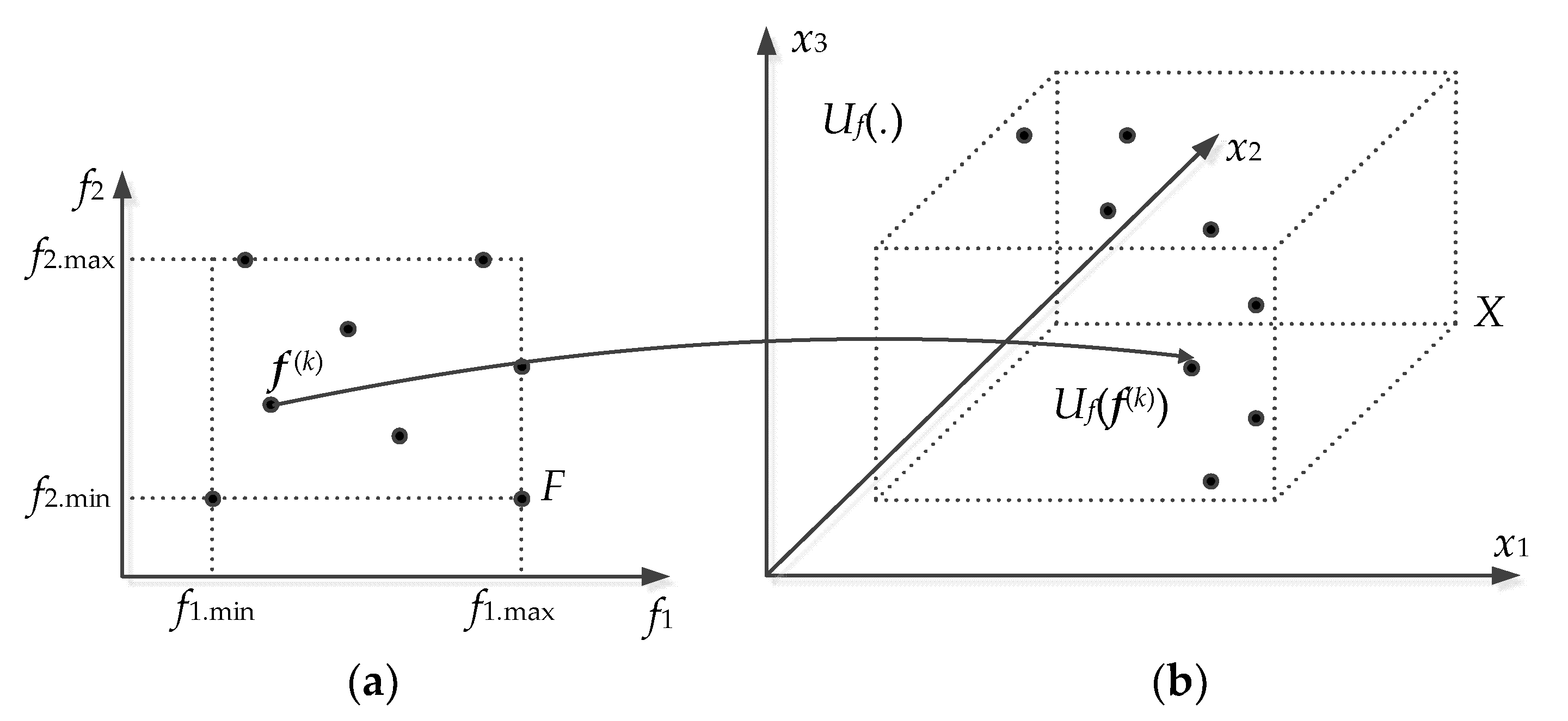
Within the proposed modeling methodology, the following two spaces are of particular importance. The first one is the standard parameter space, denoted as X. The components of the design vectors represent geometry or material parameters of the antenna being modeled. As mentioned above, conventionally, X is an interval of the form , where and are the lower and upper bounds for the design parameters, respectively. The second set is the objective space, denoted as F. Its elements are the objective vectors , which represent the antenna operating parameters (e.g., operating frequencies, bandwidth, etc.). The space F is also an interval, i.e., , where fj.min and fj.max, j = 1, …, N, are the lower and upper bounds on the objectives, respectively. The objective space F is the intended region of validity of the surrogate model to be constructed. It should be reiterated that the objectives, here, are essentially the synonyms of the figures of interest. In other words, the meaning of a particular objective vector f is that the antenna is supposed to be designed so that the performance specifications pertinent to f are achieved. For example, if the design goal is to maximize the dual-band antenna bandwidth in a symmetric manner w.r.t. the operating frequencies f1 and f2 (so that f = [f1 f2]T), then the surrogate model should cover the parameter space region that contains all designs that are optimum in the above sense for all f ∊ F.
The designs are assessed using the scalar merit function U. Similarly, as in [40], the design optimality is defined through a solution to the minimization problem
where Uf(f) stands for the design optimized w.r.t. the target objective vector f. Analytical formulation of the function U very much depends on the design task [21].
2.2. Pre-Optimized Data and Principal Component Analysis
The surrogate model domain is established using some pre-existing data, referred to as reference designs . These are the designs pre-optimized with respect to the selected objective vectors , as in Equation (1). More specifically, . In order to obtain an adequate representation of the objective space, the vectors f(j) should be distributed uniformly within F. A graphical illustration of the objective space, parameter space, and exemplary allocation of the reference designs are found in Figure 1.
We denote by the center of the reference set. Using xm, one can define the covariance matrix of the set as
We denote by , the eigenvectors of Sp. These are the principal components of the set . Their corresponding eigenvalues, denoted as λk, are the variances of the {x(k)} in the eigenspace. Without loss of generality, we can assume that the eigenvalues are given in a descending order, that is, we have . For the purpose of subsequent considerations, we also defined n × k matrices , the columns of which are the first k eigenvectors. The particular matrix, An, which contains all eigenvectors is denoted as .
2.3. Defining the Surrogate Model Domain
The set of eigenvectors provides important information about the allocation of the reference designs in the design space. This concerns both the spread and the orientation of the vectors x(k) with respect to each other. Here, we exploit this data to formally define the domain of the surrogate model. Note that each reference design x(k) can be expanded with respect to the orthogonal basis as
We also introduce some auxiliary notation
and
In (7), . Furthermore, we define the center point
Now we are in a position to define the auxiliary domain Xk as
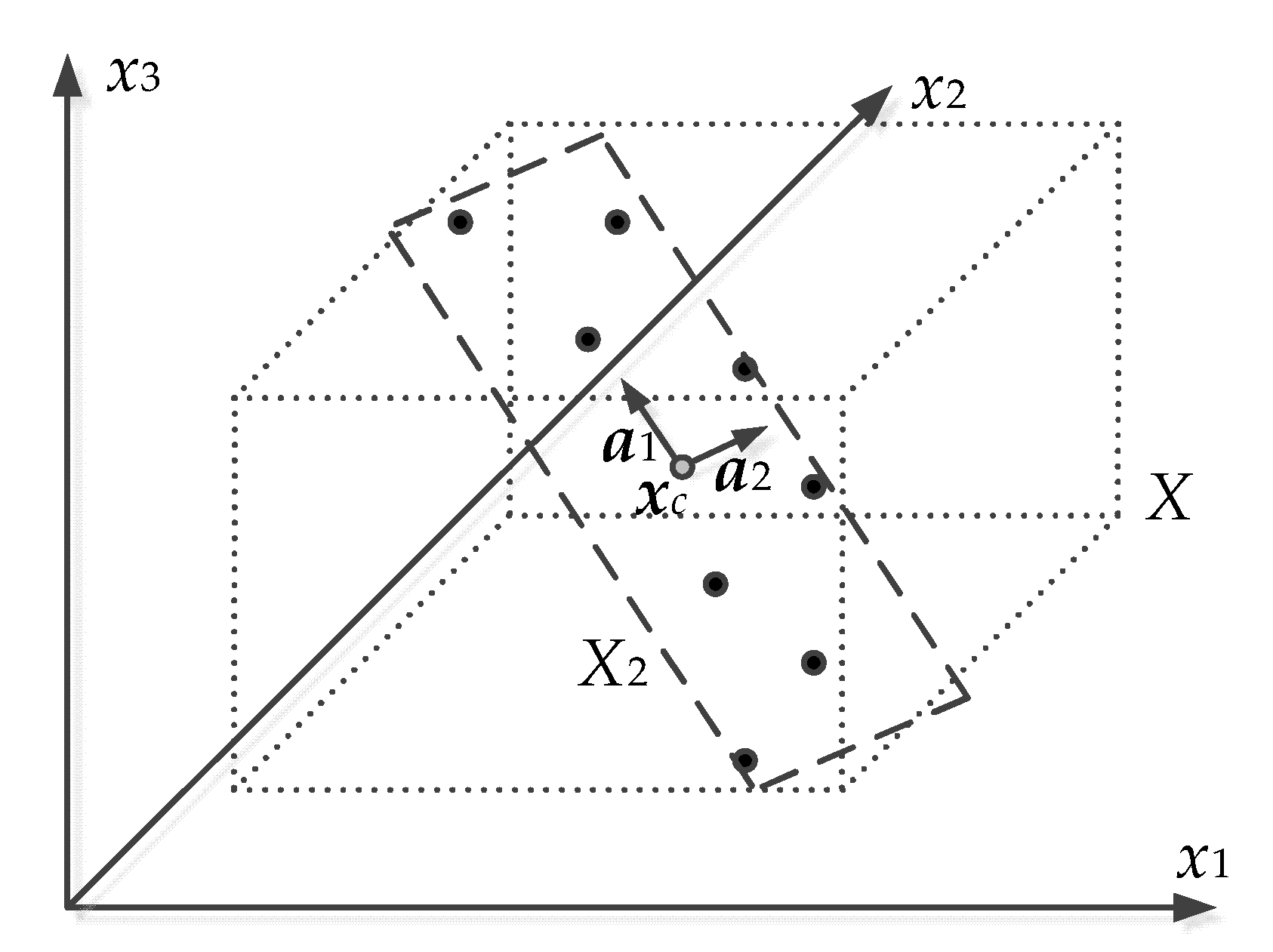
It can be observed that, by definition, Xk contains all points x(k) in the directions a1 through ak. This extends to all directions for k = n. Having chosen the value k, the domain of the surrogate model is defined as . Normally, the geometry parameters of the antenna that correspond to high-quality designs are well correlated. This means that selecting a relatively small value of k (as compared to n) should be sufficient to obtain adequate representation of the parameter space (the first k vectors aj correspond to the most important principal components). Furthermore, having k < n allows for explicit reduction of dimensionality, and, in turn, improved scalability of the surrogate in terms of the relationship between the model accuracy and the number of training data samples. A graphical illustration of the exemplary domain X2 defined as discussed in this section is shown in Figure 2.
2.4. Sampling Procedure and Model Identification
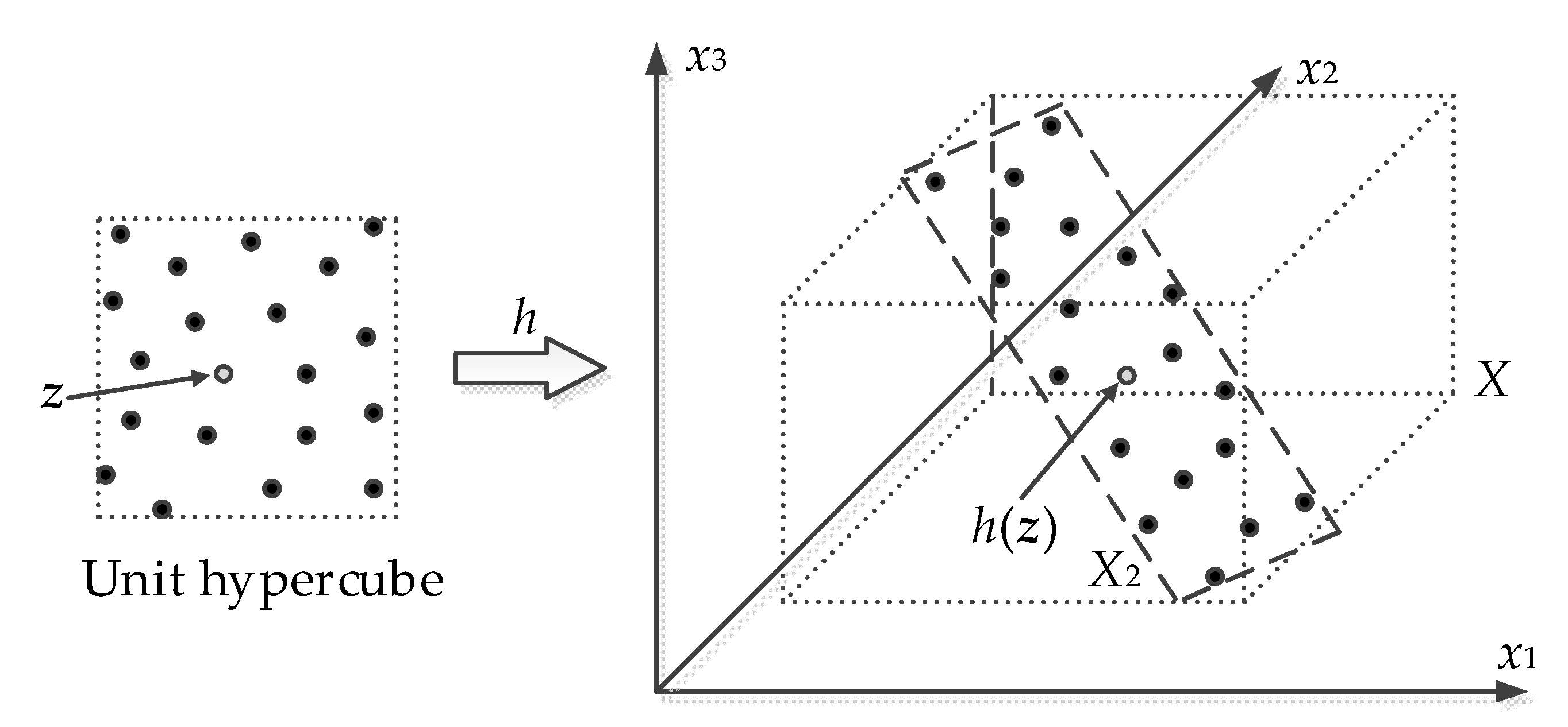
In this work, kriging interpolation [30] is used as a model identification approach, although selection of any particular modeling technique is not critical as the major computational benefits result from of the domain confinement. A practical issue is the design of experiments, i.e., the strategy for allocating the training data samples. Here, we aim at uniform sampling, which is implemented as described below. As the model domain is a k-dimensional interval in the n-dimensional parameter space, allocation of the training points is arranged in two stages. In the first step, a set of samples uniformly distributed in the unity hypercube of the dimension k is obtained using Latin hypercube sampling (LHS) [42]. These points are of the form , with . Subsequently, the samples are mapped into XS as
where the coefficients λbj have been defined in Equation (7), whereas aj are the eigenvectors of the matrix Sp (see Equation (2)). A graphical illustration of the sampling procedure is shown in Figure 3. The flow diagram of the entire modeling process is provided in Figure 4.
Formally speaking, the model domain is an intersection of the interval Xk and the original parameter space X. In practice, the vast majority of Xk is typically in X (or it is even a proper subset of X). If this is not the case, then, the samples generated according to Equation (10) that do not belong to Xk ∩ X are simply eliminated from the training set.
2.5. Design Applications: Optimizing the Surrogate
The surrogate model is supposed to facilitate the simulation-driven design procedures, the most important and common being parameter tuning. Clearly, the process should be confined to the region of validity of the surrogate, i.e., XS. From the practical point of view, it is more convenient to formally conduct the optimization process in the unity interval, further transformed onto the model domain to evaluate the antenna structure at hand. For that purpose, we employ the mapping defined in Equation (10).
Consider a target objective vector . Our goal is to solve the problem of the form of Equation (1). Using the mapping h, it can be reformulated as
It can be noted that a similar concept has been applied in [40]. An important remark is that the mapping h is surjective (in particular it is “onto” XS), which ensures that operating within the unity interval guarantees covering the entire domain of the surrogate.
3. Validation and Benchmarking
The purpose of this section is to carry out numerical validation of the presented modeling framework. Towards this end, two examples of microstrip antenna structures are investigated, namely a dual-band dipole and a ring slot antenna. Furthermore, comparisons with conventional modeling methods (specifically, kriging interpolation and radial basis functions) are provided along with the analyses of the effect of the number of training data samples on the model predictive power. Finally, application case studies are included in order to demonstrate design utility of the surrogates.
3.1. Example 1: Dual-Band Dipole Antenna
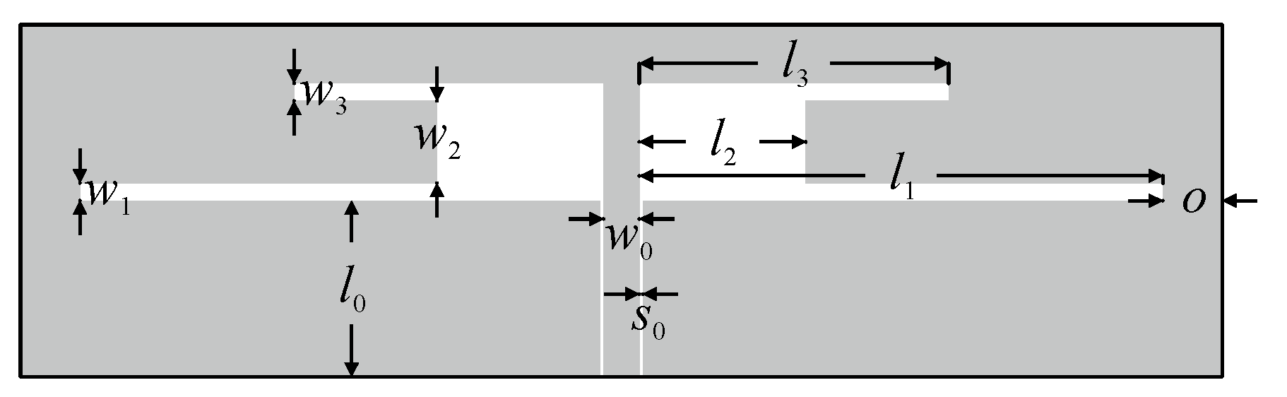
The first verification case is a dual-band dipole antenna [43]. The structure geometry is shown in Figure 5. It is realized on Rogers RO4350 substrate (εr = 3.5, h = 0.76 mm) and described by six parameters The remaining parameters are fixed as follows: . The unit for all parameters is mm. The antenna is fed by a 50 Ohm coplanar waveguide (CPW). The structure is evaluated in CST (, simulation time ~60 s).
The objective space for the surrogate is defined by the following ranges of the antenna operating frequencies: (lower band) and (upper band). The allocation of the reference designs is the same as in [40], and corresponding to: , , , , , , , (frequencies in GHz). The conventional domain X is determined using the following bounds (established as the smallest interval containing the reference designs): and . It should be emphasized that the ratios between the upper and lower bounds are considerably large, from 1.5 to 7.0 and an average of 3.1.
For the sake of verification, the proposed method is used to render the surrogates using several training datasets consisting of and samples. The assumed error measure is relative RMS error, whereas the model accuracy is estimated based on 100 random designs using the split sample approach [44]. As mentioned before, the benchmark consists of the standard kriging interpolation and radial basis function (RBF) models established in the conventional domain X. The nested kriging framework [40] is also included in the comparison set (here, with the domain thickness parameter ). The kriging surrogate employs Gaussian correlation functions, whereas RBF uses Gaussian basis function (the scaling parameter tuned through cross-validation).
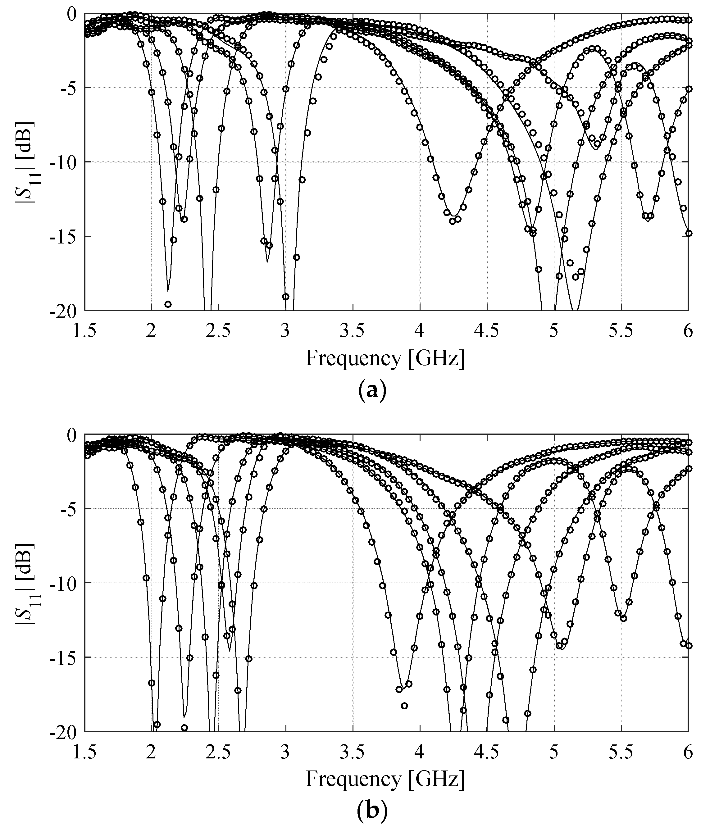
Additional experiments are conducted to investigate the scalability of the PCA-based surrogates. For that purpose, the models are constructed using different domains (see Section 2.3 for details). The selected responses of the PCA-based surrogates and the corresponding EM simulation data are shown in Figure 6. Note that the agreement between the two datasets is very good.
The numerical data on model predictive power is summarized in Table 1. The first observation is that both performance-driven approaches (nested kriging and the PCA-based method) are noticeably better than the conventional models, which indicates the importance of domain confinement. When it comes to comparing the nested kriging method with the proposed one, the two are comparable for and, on the one hand, the former shows some advantages for (full dimensionality). The reason is that the nested kriging approach accounts for the optimum design manifold geometry, which is encoded within the first-level model (see [40]). On the other hand, the proposed methodology shows its advantages when the dimensionality of the domain is diminished to or . This is especially for when the PCA-based model is considerably better than nested kriging. It should be noted that the remarkable accuracy (RMS error better than 3 percent) is achieved for as few as 50 training samples.
The question arises, whether the number of principal components required to ensure sufficient accuracy of the surrogate can be inferred beforehand, i.e., prior to acquiring data to set up the surrogate and the overall modeling routine. This can be done by analyzing the eigenvalues of the reference set. For the antenna shown in Figure 5, the normalized eigenvalues are . This indicates that only the first three principal components are important and there is no reason to go beyond or As shown in Table 1, for both cases, the PCA-based surrogate is superior over the nested kriging.
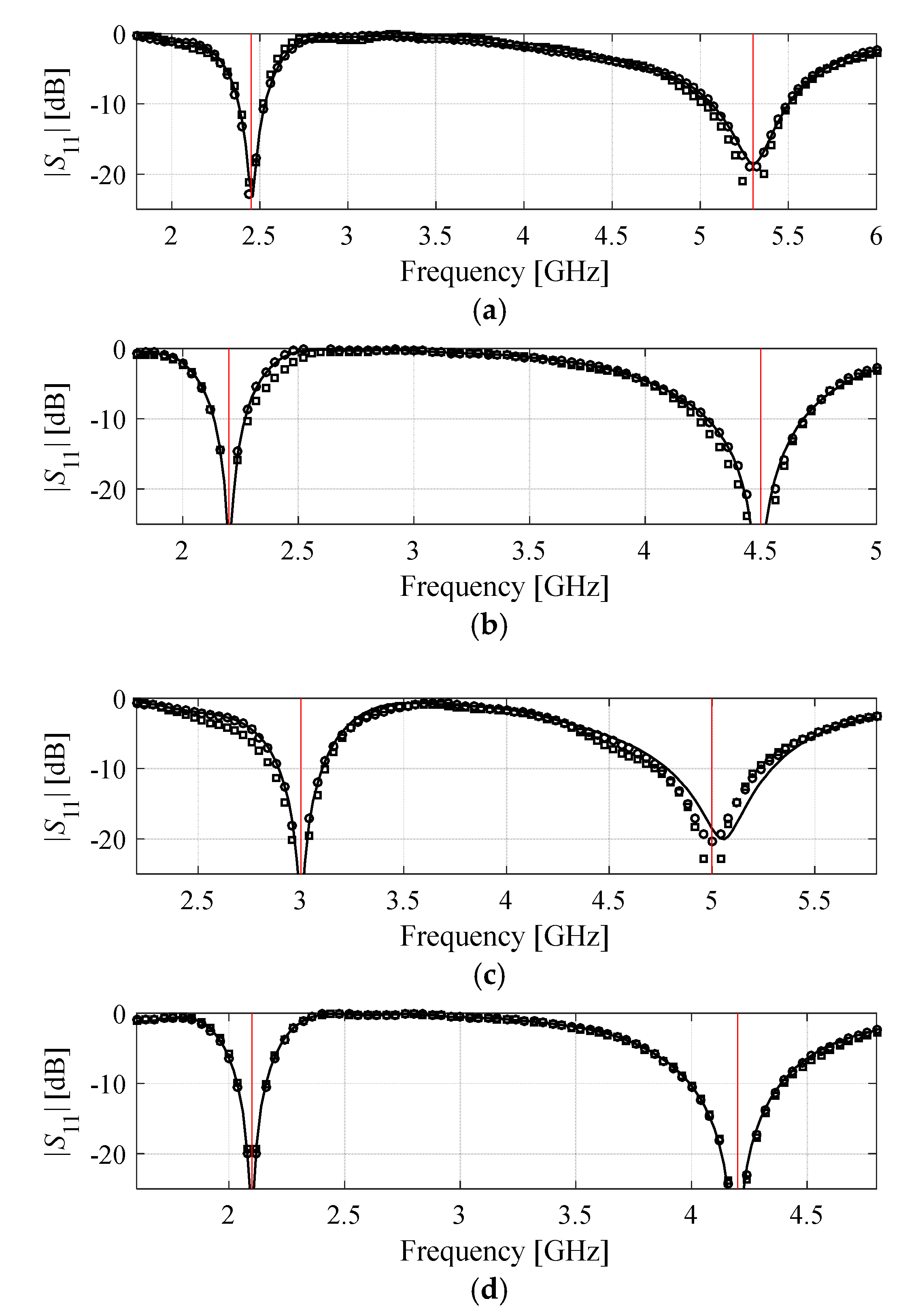
Another type of verification is executed to test the model utility. This sort of validation is necessary because, on the one hand, the surrogate is reliable within its domain, and on the other hand, the domain should accommodate a sufficiency large portion of the optimum design manifold so that the model can be effectively used to identify optimum antenna designs for the assumed objective space. This is demonstrated by running model optimization for the selected target vectors (see Table 2). In this case, we use the surrogate established in the domain . For comparison, the nested kriging model is also used. The latter does not limit the domain dimensionality and is considered to be a more flexible option. Notwithstanding, as shown in Figure 7, dimensionality reduction does not compromise the quality of the obtained designs. This indicates that it is indeed sufficient to only consider two principal components.
3.2. Example 2: Ring Slot Antenna
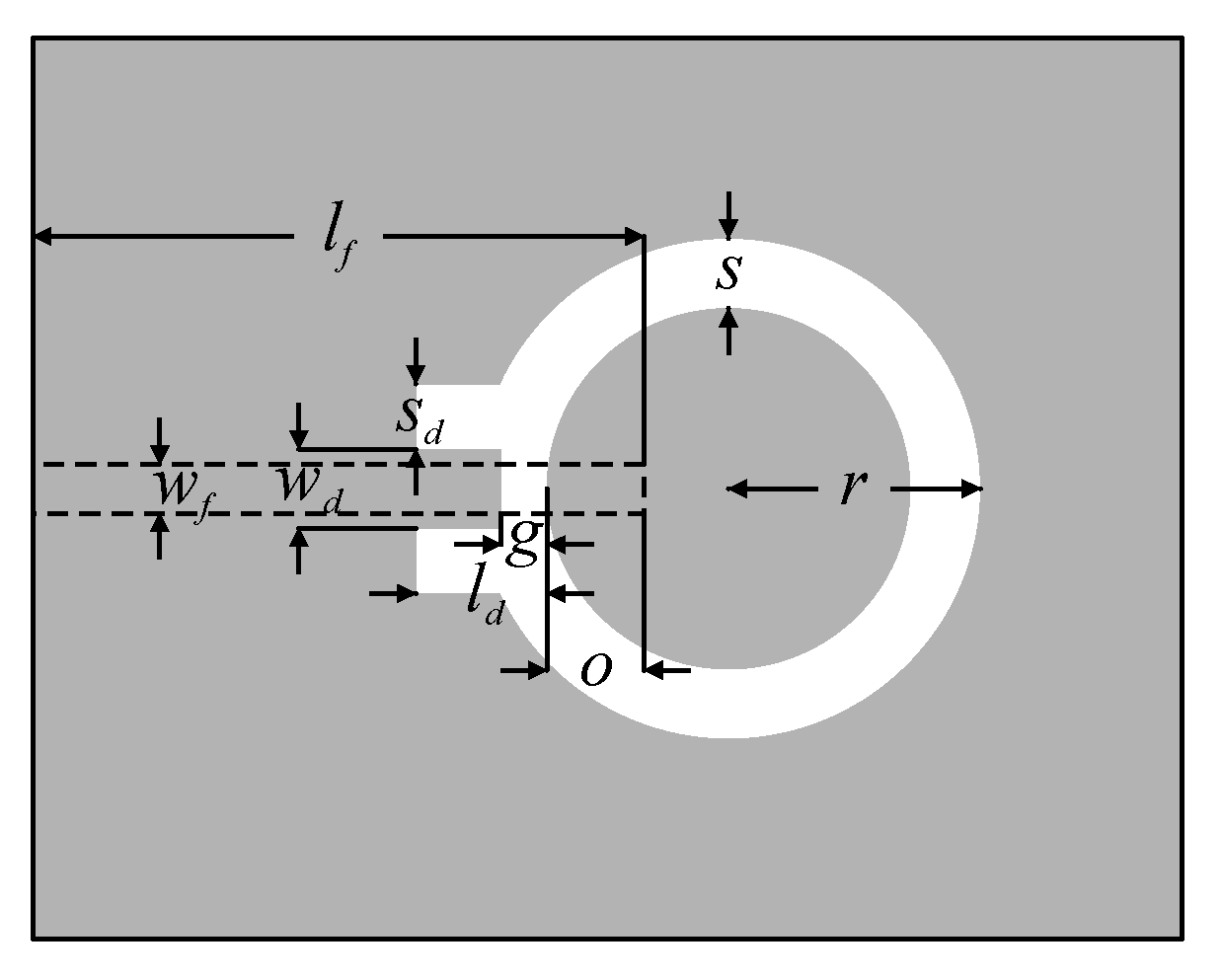
Figure 8 shows the second verification case, which is a ring slot antenna with a microstrip feed [39]. The structure is described by the following design variables . In this case, the substrate relative permittivity is one of the two figures of interest (the other is the antenna operating frequency), whereas the substrate height is set to . The antenna input impedance is , which is ensured by the appropriate adjustment of the width for the selected permittivity . Evaluation of the antenna model is performed with the use of the transient solver of CST Microwave Studio ( mesh cells, the simulation time is ).
The aim is to construct surrogate valid for the following ranges of the performance figures: (i) the antenna operating frequency and (ii) the relative substrate permittivity . The reference design set comprises ten designs , , optimal w.r.t. the following pairs of the performance figures: , , , , , , , , , and (for details see [40]). The design space is defined by: and , i.e., the lower and the upper bounds on the design variables. The bounds are based on the reference set . In this example, the number of parameters is larger, and their ranges are wider (the average ratio of the upper to lower parameter bounds is around 5.0; ranging from approximately up to ) as compared with the dual-band antenna of Section 3.1. Hence, the modeling task is considerably more difficult. The PCA-based surrogate within the confined domains () is constructed using datasets consisting of training samples. Table 3 provides the numerical results obtained within the proposed modeling framework, benchmarked against conventional kriging and RBF surrogates (set up within box-constrained domain ), as well as the nested kriging surrogate [40] set up within a constrained domain; the domain thickness is set to . The modeling error (relative RMS averaged over the testing set) is estimated with the use of a split sample method [44] (100 independent random test points are used). Figure 9 shows the responses of the EM model, along with the responses of the PCA-based surrogates and set up using 50 and 200 samples, respectively.
The modeling results, presented in Table 3, correspond to those obtained for the previous example. Here, the predictive power of the surrogates established with the use of the modeling frameworks operating within constrained domains is also significantly better than those obtained for the conventional data-driven surrogates. Moreover, the accuracies of the PCA-based surrogates and are better than that of the nested kriging surrogate. In this case, the benefits originating from domain dimensionality reduction are clearly pronounced. It should be noted that for such a truly challenging test case, the modeling errors obtained for are indeed very low (below 6 percent for 50 samples).
The predictive power of the nested kriging model and the PCA-based surrogate are close to each other for . For , the quality of the nested kriging model is superior, due to the fact that the surrogate domain provides a better account for the optimum design set for the considered antenna. Similar to the previous case, the analysis of the eigenvalues of the reference design set can be used to establish the necessary number of principal components. Here, we have . One can observe a significant difference between the first and the remaining eigenvalues, as well as that the fourth one is less than three percent of the first. According to this, we can conclude that using or is sufficient.
Design utility of the proposed surrogate model is corroborated through the application case studies as described below. The main point is to make sure that reducing the surrogate model domain dimensionality does not have detrimental effects on the design quality that can be identified through model optimization. For the sake of comparison, the antenna optimization is also carried out using the nested kriging surrogate [38], employed as a benchmark, and the latter retaining full dimensionality of the parameter space. The results obtained for the selected operating conditions are summarized in Table 4. The proposed surrogate is rendered using two principal components, i.e., for . A graphical illustration of the antenna characteristics is shown in Figure 10. Note that the proposed surrogate and the benchmark lead to comparable results. This demonstrates that the PCA-based surrogate is indeed a reliable tool for antenna design closure.
4. Conclusions
In the paper, a novel technique for surrogate modeling of antenna structures has been proposed. Our methodology follows the generic concept of performance-driven modeling, where the surrogate domain is confined using an auxiliary set of reference designs optimized with respect to the problem-specific figures of interest. Here, the domain for rendering the surrogate is constructed using the selected principal components of the reference designs, generated from their covariance matrix. This approach exhibits several important advantages. In particular, it permits a significant reduction of the parameter space region that needs to be sampled, in terms of both the parameter ranges and the dimensionality. The latter is controlled by the number of principal components utilized to define the domain and can be determined by analyzing the reference set eigenvalues. At the same time, the model domain accommodates all parameter space subsets that are important from the point of view of the considered performance figures. This is a keystone for the modeling process reliability.
Comprehensive benchmarking demonstrates that the proposed approach is superior over both conventional modeling methods (kriging, radial basis function interpolation) but also the recently reported nested kriging modeling. When restricting the model domain dimensionality to two or three (otherwise sufficient as determined by the eigenvalue analysis), the surrogate can be constructed to cover wide ranges of operating conditions and to feature the predictive power as good as a few percent in terms of the relative RMS error, while using fifty or one hundred training samples. This is where conventional frameworks fail to produce reliable surrogates even with several hundred data points, which is particularly evident for the second (more challenging) example of the ring-slot antenna.
In the context of practical applications, the proposed methodology is convenient, because the surrogate model domain is homeomorphic with the unity interval. This enables straightforward implementation of the design of experiments (sampling) and, more importantly, easy arrangement of parametric optimization as demonstrated through examples. Overall, the presented technique can be considered to be a convenient supplementary antenna design tool, especially when certain prior information (e.g., in the form of the designs obtained for various performance specifications) is already available. Additionally, it can also be employed to render reusable models for repetitive design (e.g., for different operating frequencies, substrates, etc.) of a given antenna structure.
Author Contributions
Conceptualization, S.K. and A.P.-D.; methodology, S.K. and A.P.-D.; software, S.K. and A.P.-D.; validation, S.K. and A.P.-D.; formal analysis, S.K.; investigation, S.K. and A.P.-D.; resources, S.K.; data curation, S.K. and A.P.-D.; writing—original draft preparation, S.K. and A.P.-D.; writing—review and editing, S.K.; visualization, S.K. and A.P.-D.; supervision, S.K.; project administration, S.K.; funding acquisition, S.K. All authors have read and agreed to the published version of the manuscript.
Funding
This work was supported in part by the Icelandic Centre for Research (RANNIS) grant 174114051, and by the National Science Centre of Poland grant 2017/27/B/ST7/00563.
Acknowledgments
The authors thank Dassault Systemes, France, for making the CST Microwave Studio available.
Conflicts of Interest
The authors declare no conflict of interest. The funders had no role in the design of the study; in the collection, analyses, or interpretation of data; in the writing of the manuscript, or in the decision to publish the results.
References
- Guo, J.; Cui, L.; Li, C.; Sun, B. Side-edge frame printed eight-port dual-band antenna array for 5G smartphone applications. IEEE Trans. Ant. Prop. 2018, 66, 7412–7417. [Google Scholar] [CrossRef]
- Liu, Y.; Zhang, J.; Ren, A.; Wang, H.; Sim, C.Y.D. TCM-based hepta-band antenna with small clearance for metal-rimmed phone applications. IEEE Trans. Ant. Wirel. Prop. Lett. 2018, 18, 717–721. [Google Scholar] [CrossRef]
- Liao, W.J.; Hsieh, C.Y.; Dai, B.Y.; Hsiao, B.R. Inverted-F/slot integrated dual-band four-antenna system for WLAN access point. IEEE Ant. Wirel. Prop. Lett. 2015, 14, 847–850. [Google Scholar] [CrossRef]
- Kumar, A.; Ansari, A.Q.; Kanaujia, B.; Kishor, J.; Kumar, S. An ultra-compact two-port UWB-MIMO antenna with dual band-notched characteristics. AEU Int. J. Electr. Comm. 2019, 114, 152997. [Google Scholar] [CrossRef]
- Majidzadeh, M. Linear and circular polarization radiation through a modified 270° square ring-fed 2×2 array antenna. AEU Int. J. Electr. Comm. 2019, 98, 164–173. [Google Scholar] [CrossRef]
- Wu, J.; Sarabandi, K. Compact omnidirectional circularly polarized antenna. IEEE Trans. Ant. Prop. 2017, 65, 1550–1557. [Google Scholar] [CrossRef]
- Kurgan, P.; Koziel, S. Selection of circuit geometry for miniaturized microwave components based on concurrent optimization of performance and layout area. AEU Int. J. Electr. Comm. 2019, 108, 287–294. [Google Scholar] [CrossRef]
- Lakbakhsh, A.; Afzal, M.U.; Esselle, K.P. Multiobjective particle swarm optimization to design a time-delay equalizer metasurface for an electromagnetic band-gap resonator antenna. IEEE Ant. Wirel. Prop. Lett. 2017, 16, 915. [Google Scholar]
- Zhang, J.; Zhang, C.; Feng, F.; Zhang, W.; Ma, J.; Zhang, Q.J. Polynomial chaos-based approach to yield-driven EM optimization. IEEE Trans. Microw. Theory Tech. 2018, 66, 3186–3199. [Google Scholar] [CrossRef]
- Hassan, A.S.O.; Abdel-Malek, H.L.; Mohamed, A.S.A.; Abuelfadl, T.M.; Elqenawy, A.E. Statistical design centering of RF cavity linear accelerator via non-derivative trust region optimization. In Proceedings of the 2015 IEEE MTT-S International Conference on Numerical Electromagnetic and Multiphysics Modeling and Optimization (NEMO), Ottawa, ON, Canada, 11–14 August 2015; pp. 1–3. [Google Scholar]
- Kouassi, A.; Nguyen-Trong, N.; Kaufmann, T.; Lallechere, S.; Bonnet, P.; Fumeaux, C. Reliability-aware optimization of a wideband antenna. IEEE Trans. Ant. Prop. 2016, 64, 450–460. [Google Scholar] [CrossRef]
- Nocedal, J.; Wright, S. Numerical Optimization, 2nd ed.; Springer: New York, NY, USA, 2006. [Google Scholar]
- Darvish, A.; Ebrahimzadeh, A. Improved fruit-fly optimization algorithm and its applications in antenna array synthesis. IEEE Trans. Ant. Prop. 2018, 66, 1756–1766. [Google Scholar] [CrossRef]
- Dong, J.; Li, Q.; Deng, L. Fast multi-objective optimization of multi-parameter antenna structures based on improved MOEA/D with surrogate-assisted model. AEU Int. J. Electr. Comm. 2017, 72, 192–199. [Google Scholar] [CrossRef] [Green Version]
- Koziel, S.; Mosler, F.; Reitzinger, S.; Thoma, P. Robust microwave design optimization using adjoint sensitivity and trust regions. Int. J. RF Microw. CAE 2012, 22, 10–19. [Google Scholar] [CrossRef]
- Wang, J.; Yang, X.S.; Wang, B.Z. Efficient gradient-based optimization of pixel antenna with large-scale connections. IET Microw. Ant. Prop. 2018, 12, 385–389. [Google Scholar] [CrossRef]
- Koziel, S.; Pietrenko-Dabrowska, A. Expedited optimization of antenna input characteristics with adaptive Broyden updates. Eng. Comp. 2020, 37, 851–862. [Google Scholar] [CrossRef]
- Koziel, S.; Pietrenko-Dabrowska, A. Variable-fidelity simulation models and sparse gradient updates for cost-efficient optimization of compact antenna input characteristics. Sensors 2019, 19, 1806. [Google Scholar] [CrossRef] [Green Version]
- Zhang, Y.; Zhao, Z.; Wang, J.; Dan, G. Antenna array beam pattern synthesis based on trust region method. In Proceedings of the 2014 IEEE 17th International Conference on Computational Science and Engineering, Chengdu, China, 19–21 December 2014; pp. 859–862. [Google Scholar]
- Bandler, J.W.; Mohamed, A.S.; Bakr, M.H. TLM-based modeling and design exploiting space mapping. IEEE Trans. Microw. Theory Techn. 2005, 53, 2801–2811. [Google Scholar] [CrossRef] [Green Version]
- Tu, S.; Cheng, Q.S.; Zhang, Y.; Bandler, J.W.; Nikolova, N.K. Space mapping optimization of handset antennas exploiting thin-wire models. IEEE Trans. Ant. Propag. 2013, 61, 3797–3807. [Google Scholar] [CrossRef]
- Koziel, S.; Leifsson, L. Simulation-Driven Design by Knowledge-Based Response Correction Techniques; Springer: New York, NY, USA, 2016. [Google Scholar]
- Koziel, S.; Unnsteinsson, S.D. Expedited design closure of antennas by means of trust-region-based adaptive response scaling. IEEE Ant. Wirel. Prop. Lett. 2018, 17, 1099–1103. [Google Scholar] [CrossRef]
- Su, Y.; Lin, J.; Fan, Z.; Chen, R. Shaping optimization of double reflector antenna based on manifold mapping. In Proceedings of the 2017 International Applied Computational Electromagnetics Society Symposium (ACES), Firenze, Italy, 1–4 August 2017. [Google Scholar]
- Easum, J.A.; Nagar, J.; Werner, D.H. Multi-objective surrogate-assisted optimization applied to patch antenna design. In Proceedings of the 2017 IEEE International Symposium on Antennas and Propagation & USNC/URSI National Radio Science Meeting, San Diego, CA, USA, 9–14 July 2017; pp. 339–340. [Google Scholar]
- Hassan, A.K.; Etman, A.S.; Soliman, E.A. Optimization of a novel nano antenna with two radiation modes using kriging surrogate models. IEEE Photonics J. 2018, 10, 4800807. [Google Scholar] [CrossRef]
- de Villiers, D.I.L.; Couckuyt, I.; Dhaene, T. Multi-objective optimization of reflector antennas using kriging and probability of improvement. In Proceedings of the 2017 IEEE International Symposium on Antennas and Propagation & USNC/URSI National Radio Science Meeting, San Diego, CA, USA, 9–14 July 2017; pp. 985–986. [Google Scholar]
- Chen, Y.; Tian, Y.B.; Qiang, Z.; Xu, L. Optimisation of reflection coefficient of microstrip antennas based on KBNN exploiting GPR model. IET Microw. Ant. Prop. 2018, 12, 602–606. [Google Scholar] [CrossRef]
- Koziel, S. Fast simulation-driven antenna design using response-feature surrogates. Int. J. RF Microw. CAE 2015, 25, 394–402. [Google Scholar] [CrossRef]
- Simpson, T.W.; Pelplinski, J.D.; Koch, P.N.; Allen, J.K. Metamodels for computer-based engineering design: Survey and recommendations. Eng. Comput. 2001, 17, 129–150. [Google Scholar] [CrossRef] [Green Version]
- Chávez-Hurtado, J.L.; Rayas-Sánchez, J.E. Polynomial-based surrogate modeling of RF and microwave circuits in frequency domain exploiting the multinomial theorem. IEEE Trans. Microw. Theory Tech. 2016, 64, 4371–4381. [Google Scholar] [CrossRef] [Green Version]
- Jacobs, J.P. Characterization by Gaussian processes of finite substrate size effects on gain patterns of microstrip antennas. IET Microw. Ant. Prop. 2016, 10, 1189–1195. [Google Scholar] [CrossRef] [Green Version]
- Kabir, H.; Wang, Y.; Yu, M.; Zhang, Q.J. Neural network inverse modeling and applications to microwave filter design. IEEE Trans. Microw. Theory Tech. 2008, 56, 867–879. [Google Scholar] [CrossRef]
- Smola, A.J.; Schölkopf, B. A tutorial on support vector regression. Stat. Comput. 2004, 14, 199–222. [Google Scholar] [CrossRef] [Green Version]
- Leary, S.; Bhaskar, A.; Keane, A. Optimal orthogonal-array-based latin hypercubes. J. Appl. Stat. 2003, 30, 585–598. [Google Scholar] [CrossRef] [Green Version]
- Santner, T.J.; Williams, B.J.; Notz, W.I. Space-filling designs for computer experiments. In The Design and Analysis of Computer Experiments; Springer Series in Statistics; Springer: New York, NY, USA, 2003; pp. 121–161. [Google Scholar]
- Crombecq, K.; Laermans, E.; Dhaene, T. Efficient space-filling and non-collapsing sequential design strategies for simulation-based modeling. Eur. J. Oper. Res. 2011, 214, 683–696. [Google Scholar] [CrossRef] [Green Version]
- Koziel, S. Low-cost data-driven surrogate modeling of antenna structures by constrained sampling. IEEE Ant. Wirel. Propag. Lett. 2017, 16, 461–464. [Google Scholar] [CrossRef]
- Koziel, S.; Sigurdsson, A.T. Triangulation-based constrained surrogate modeling of antennas. IEEE Trans. Ant. Prop. 2017, 66, 4170–4179. [Google Scholar] [CrossRef]
- Koziel, S.; Pietrenko-Dabrowska, A. Performance-based nested surrogate modeling of antenna input characteristics. IEEE Trans. Ant. Prop. 2019, 67, 2904–2912. [Google Scholar] [CrossRef]
- Jolliffe, I.T. Principal Component Analysis, 2nd ed.; Springer: New York, NY, USA, 2002. [Google Scholar]
- Beachkofski, B.; Grandhi, R. Improved Distributed Hypercube Sampling; Paper AIAA 2002–1274; American Institute of Aeronautics and Astronautics: Reston, VA, USA, 2002. [Google Scholar]
- Chen, Y.-C.; Chen, S.-Y.; Hsu, P. Dual-band slot dipole antenna fed by a coplanar waveguide. In Proceedings of the 2006 IEEE Antennas and Propagation Society International Symposium, Albuquerque, NM, USA, 9–14 July 2006; pp. 3589–3592. [Google Scholar]
- Queipo, N.V.; Haftka, R.T.; Shyy, W.; Goel, T.; Vaidynathan, R.; Tucker, P.K. Surrogate based analysis and optimization. Prog. Aerosp. Sci. 2005, 41, 1–28. [Google Scholar] [CrossRef] [Green Version]
Figure 1.
The major components of the modeling process. (a) Objective space (here, in two dimensions) consisting of performance figure vectors (e.g., operating frequencies of the system at hand); (b) Parameter space (here, in three dimensions) consisting of design vectors (typically, geometry parameters). Each point f in the objective space F has its representation in the parameter space Uf(f), which correspond to the design optimized w.r.t. the assumed merit function Uf(.). The particular objective vectors shown in the picture are the reference designs, later utilized to define the surrogate model domain.

Figure 2.
Graphical illustration of the principal components of the reference set corresponding to the parameter space shown in Figure 1. The center point xc defined by Equation (8) is marked as the gray circle. Using a1 and a2, an example surrogate domain is defined as XS = X2.
Figure 2.
Graphical illustration of the principal components of the reference set corresponding to the parameter space shown in Figure 1. The center point xc defined by Equation (8) is marked as the gray circle. Using a1 and a2, an example surrogate domain is defined as XS = X2.

Figure 3.
Graphical illustration of the sampling procedure within the surrogate model domain. An auxiliary set of samples {zk} allocated in the unity interval using Latin hypercube sampling is transformed into the surrogate domain (here, X2) by means of the one-to-one mapping h of Equation (10).
Figure 3.
Graphical illustration of the sampling procedure within the surrogate model domain. An auxiliary set of samples {zk} allocated in the unity interval using Latin hypercube sampling is transformed into the surrogate domain (here, X2) by means of the one-to-one mapping h of Equation (10).

Figure 4.
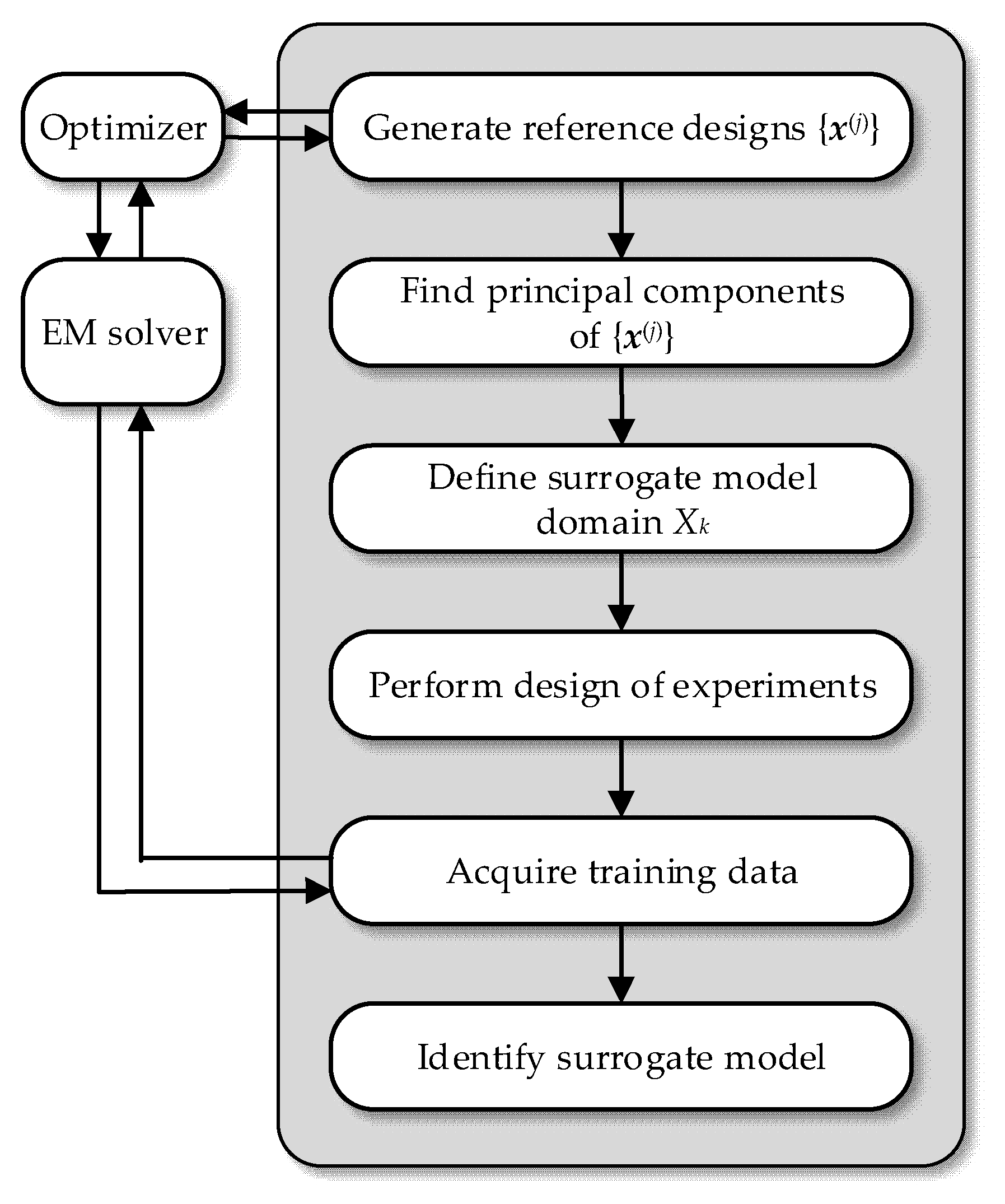
Surrogate modeling flow according to the proposed framework. The major components of the procedure include acquisition of the reference designs (see Section 2.1), obtaining the principal components of the reference set (see Section 2.2), definition of the surrogate model domain (see Section 2.3), as well as domain sampling and identification of the surrogate (see Section 2.4).
Figure 4.
Surrogate modeling flow according to the proposed framework. The major components of the procedure include acquisition of the reference designs (see Section 2.1), obtaining the principal components of the reference set (see Section 2.2), definition of the surrogate model domain (see Section 2.3), as well as domain sampling and identification of the surrogate (see Section 2.4).

Figure 5.
Dual-band dipole antenna: geometry [43].
Figure 5.
Dual-band dipole antenna: geometry [43].

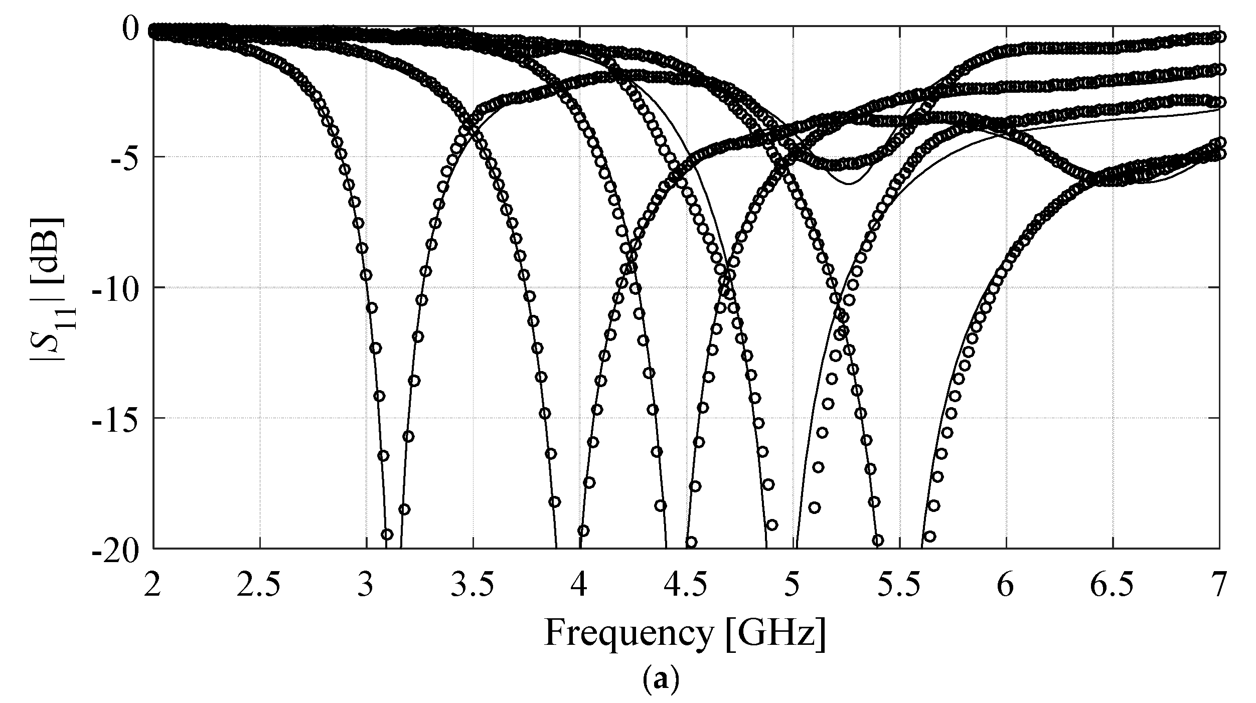
Figure 6.
Reflection characteristics of the antenna of Figure 5 at the selected test locations, i.e., full-wave electromagnetic simulation response (—) and the proposed PCA-based surrogate (o). (a) Surrogate model established using two principal components (XS = X2) and 50 training data samples; (b) Surrogate established using three principal components (XS = X3) and 200 training data samples.

Figure 7.
Reflection characteristics of the antenna of Figure 5, i.e., PCA-based surrogate (o), nested kriging surrogate [40] (□), and full-wave simulation at the design rendered through optimization of the PCA-based model (–). The following target vectors were considered: (a) f1 = 2.45 GHz, f2 = 5.3 GHz, (b) f1 = 2.2 GHz, f2 = 4.5 GHz, (c) f1 = 3.0 GHz, f2 = 5.0 GHz, and (d) f1 = 2.1 GHz, f2 = 4.2 GHz. Vertical lines denote the target operating frequencies of the antenna.

Figure 8.
Geometry of the ring slot antenna [43]. The feeding line marked using the dashed line.
Figure 8.
Geometry of the ring slot antenna [43]. The feeding line marked using the dashed line.

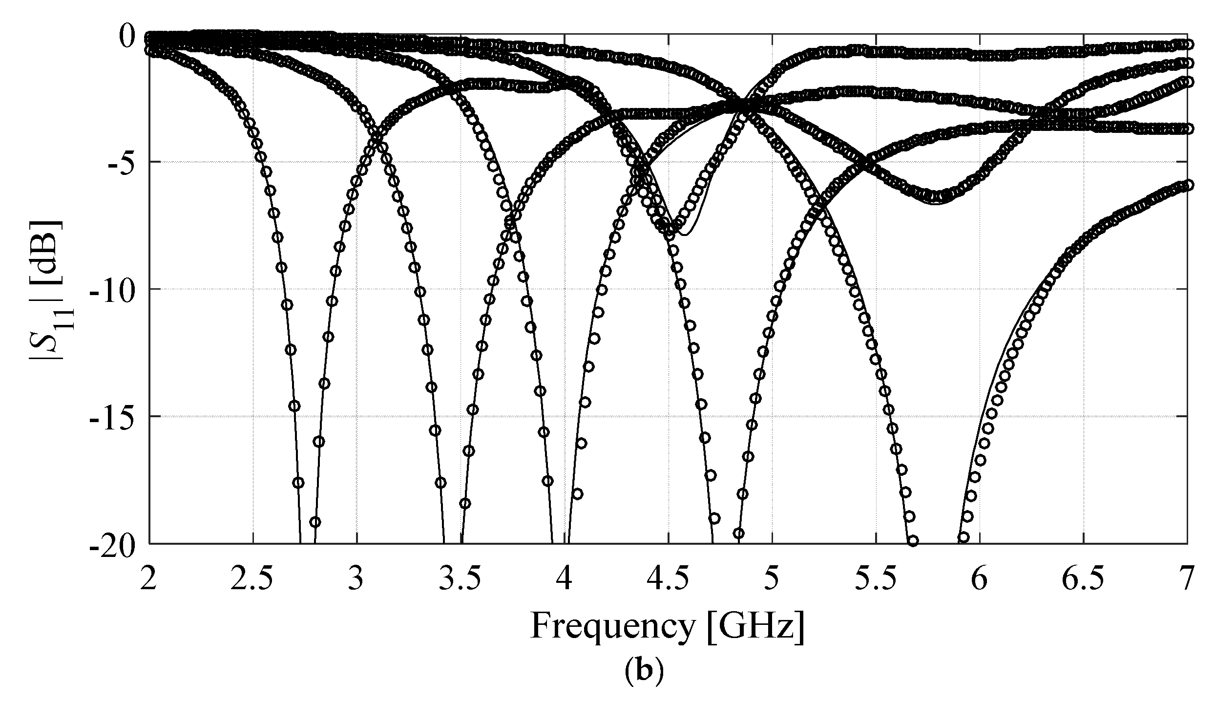
Figure 9.
Reflection characteristics of the antenna of Figure 8 at the following selected test locations: full-wave electromagnetic simulation response (–), and the proposed PCA-based surrogate (o). (a) Surrogate model established using two principal components (XS = X2) and 50 training data samples; (b) Surrogate established using three principal components (XS = X3) and 200 training data samples.


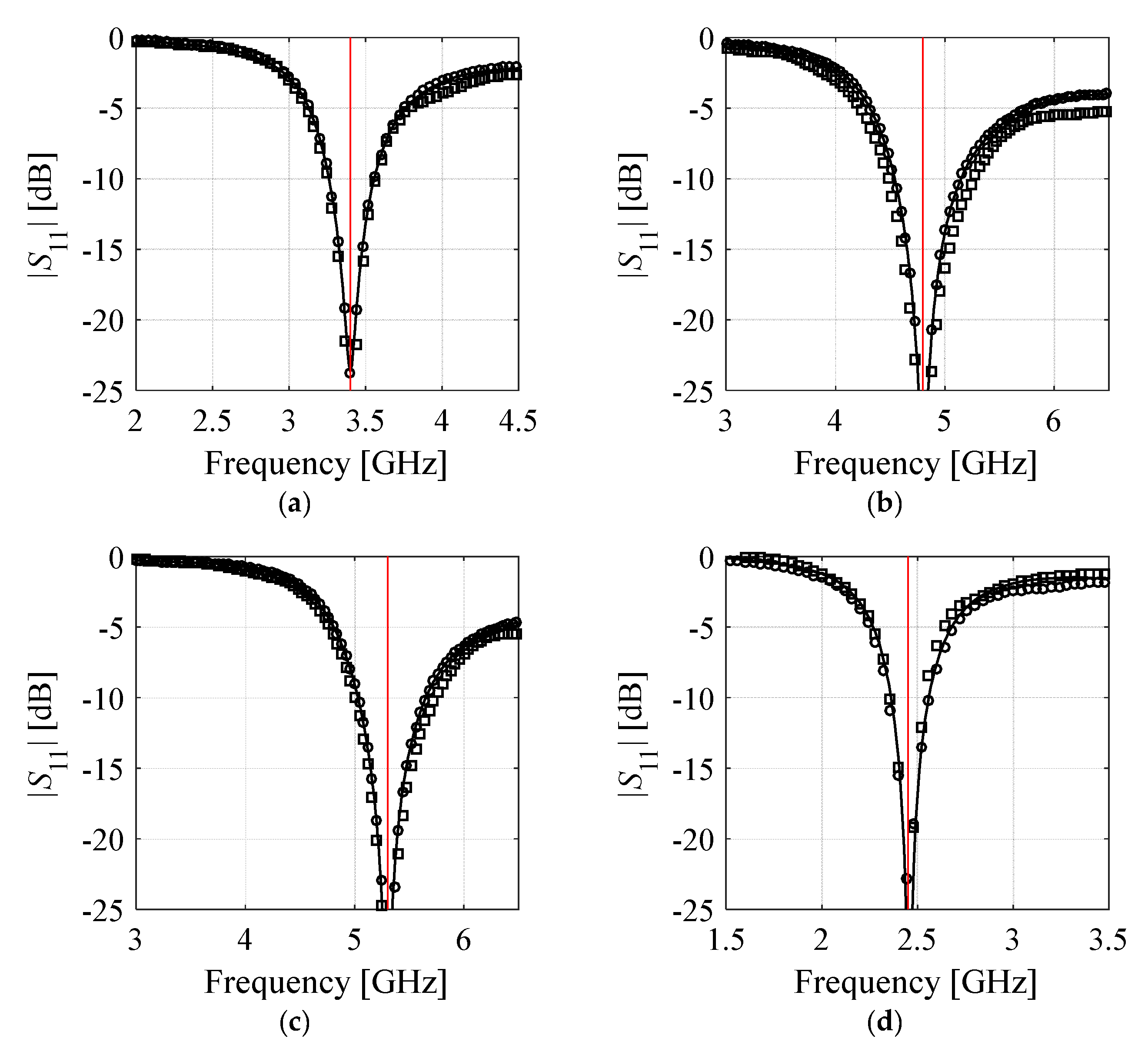
Figure 10.
Reflection characteristics of the antenna of Figure 8. PCA-based surrogate (o); nested kriging surrogate [37] (□); and full-wave simulation at the design rendered through optimization of the PCA-based model (–). The following target vectors were considered: (a) f0 = 3.4 GHz, εr = 3.5, (b) f0 = 4.8 GHz, εr = 2.2, (c) f0= 5.3 GHz, εr = 3.5, (d) f0 = 2.45 GHz, εr = 4.3. Vertical lines denote the target operating frequencies of the antenna.


Table 1.
Surrogate model accuracy and benchmarking for antenna of Figure 5.
Table 1.
Surrogate model accuracy and benchmarking for antenna of Figure 5.
| Number of Training Samples | Relative RMS Error | ||||||
|---|---|---|---|---|---|---|---|
| Conventional Models | Nested Kriging Model [37] | Proposed Model (Domain Confinement with PCA) | |||||
| Kriging | RBF | k = 2 | k = 3 | k = 4 | k = 6 | ||
| 50 | 21.7% | 24.9% | 9.9% | 2.9% | 8.6% | 11.7% | 15.9% |
| 100 | 17.3% | 19.8% | 6.4% | 1.5% | 5.2% | 8.6% | 11.0% |
| 200 | 12.6% | 14.3% | 4.4% | 1.4% | 2.9% | 5.8% | 8.1% |
| 400 | 9.3% | 10.5% | 3.8% | 1.2% | 1.9% | 4.3% | 5.8% |
| 800 | 7.2% | 8.7% | 3.4% | 1.1% | 1.5% | 3.0% | 4.6% |
Table 2.
Application case studies (parameter tuning) for antenna of Figure 5.
Table 2.
Application case studies (parameter tuning) for antenna of Figure 5.
| Target Operating Conditions | Geometry Parameter Values [mm] | ||||||
|---|---|---|---|---|---|---|---|
| f1 [GHz] | f2 [GHz] | l1 | l2 | l3 | w1 | w2 | w3 |
| 2.45 | 5.30 | 33.1 | 8.76 | 17.9 | 0.31 | 2.70 | 1.98 |
| 2.20 | 4.50 | 34.2 | 5.76 | 18.3 | 0.47 | 4.21 | 1.75 |
| 3.00 | 5.00 | 29.7 | 11.10 | 20.3 | 0.33 | 2.47 | 1.16 |
| 2.10 | 4.20 | 35.4 | 5.30 | 19.0 | 0.54 | 4.83 | 1.68 |
Table 3.
Surrogate model accuracy and benchmarking for antenna of Figure 8.
Table 3.
Surrogate model accuracy and benchmarking for antenna of Figure 8.
| Number of Training Samples | Relative RMS Error | ||||||
|---|---|---|---|---|---|---|---|
| Conventional Models | Nested Kriging Model [37] | Proposed Model (Domain Confinement with PCA) | |||||
| Kriging | RBF | k = 2 | k = 3 | k = 4 | k = 6 | ||
| 50 | 56.9% | 61.0% | 19.4% | 5.7% | 18.0% | 26.9% | 29.6% |
| 100 | 50.8% | 53.2% | 12.9% | 2.2% | 9.4% | 15.9% | 23.4% |
| 200 | 35.8% | 37.9% | 7.7% | 1.9% | 5.5% | 9.8% | 14.3% |
| 400 | 31.5% | 34.1% | 5.1% | 1.3% | 2.7% | 5.4% | 9.6% |
| 800 | 25.6% | 27.2% | 3.7% | 0.8% | 2.1% | 3.9% | 7.3% |
Table 4.
Application case studies (parameter tuning) for the antenna of Figure 8.
Table 4.
Application case studies (parameter tuning) for the antenna of Figure 8.
| Target Operating Conditions | Geometry Parameter Values [mm] | ||||||||
|---|---|---|---|---|---|---|---|---|---|
| f0 [GHz] | ε | lf | ld | wd | r | s | sd | o | g |
| 3.4 | 3.5 | 25.2 | 5.82 | 1.25 | 11.6 | 4.81 | 3.04 | 4.74 | 1.08 |
| 4.8 | 2.2 | 22.6 | 5.12 | 0.58 | 9.66 | 4.01 | 4.08 | 5.17 | 1.46 |
| 5.3 | 3.5 | 22.9 | 4.59 | 0.45 | 8.48 | 3.57 | 4.61 | 5.14 | 1.76 |
| 2.45 | 4.3 | 27.9 | 6.82 | 2.02 | 14.23 | 5.87 | 1.67 | 4.29 | 0.53 |
© 2020 by the authors. Licensee MDPI, Basel, Switzerland. This article is an open access article distributed under the terms and conditions of the Creative Commons Attribution (CC BY) license (http://creativecommons.org/licenses/by/4.0/).
Share and Cite
MDPI and ACS Style
Pietrenko-Dabrowska, A.; Koziel, S. Reliable Surrogate Modeling of Antenna Input Characteristics by Means of Domain Confinement and Principal Components. Electronics 2020, 9, 877. https://doi.org/10.3390/electronics9050877
AMA Style
Pietrenko-Dabrowska A, Koziel S. Reliable Surrogate Modeling of Antenna Input Characteristics by Means of Domain Confinement and Principal Components. Electronics. 2020; 9(5):877. https://doi.org/10.3390/electronics9050877
Chicago/Turabian StylePietrenko-Dabrowska, Anna, and Slawomir Koziel. 2020. "Reliable Surrogate Modeling of Antenna Input Characteristics by Means of Domain Confinement and Principal Components" Electronics 9, no. 5: 877. https://doi.org/10.3390/electronics9050877
Note that from the first issue of 2016, this journal uses article numbers instead of page numbers. See further details here.