An Integrated Cooling Jet and Air Curtain System for Stadiums in Hot Climates


Department of Architecture and Built Environment, University of Nottingham, Nottingham NG7 2RD, UK
*
Author to whom correspondence should be addressed.
Atmosphere 2020, 11(5), 546; https://doi.org/10.3390/atmos11050546
Submission received: 27 April 2020
/
Revised: 18 May 2020
/
Accepted: 22 May 2020
/
Published: 25 May 2020
(This article belongs to the Section Air Quality and Human Health)
Abstract
:The 2022 FIFA World Cup brings Qatar great challenges in terms of minimizing the cooling energy consumption and providing thermal comfort for both spectators and players. This paper presents comparisons among the results of thermal and wind environment modelling of a semi-outdoor stadium under three different cooling configurations and a baseline configuration without cooling using the Computational Fluid Dynamics (CFD) tool ANSYS Fluent 18.2. The three cooling configurations are: (1) vertical jets only above upper tiers, (2) vertical jets above upper tiers and horizontal jets at the back of lower tiers and around the pitch, (3) integrated vertical jets above upper tiers, horizontal jets at the back of lower tiers and air curtains at gates. De-coupled solar radiation simulations are implemented using the solar irradiance data in Doha under fair weather conditions method in Fluent in order to capture realistic thermal boundary conditions for the ground, stadium and surrounding buildings. On the basis of the set conditions, the results show that air curtains, employed in configuration 3 are effective in preventing the penetration of hot outside air through the gates of the stadium, which is an existing issue for stadiums in hot climates, and also contribute to lower energy consumption per match than the other configurations of cooling jets. The results presented in this study are useful not only for future design and retrofits of stadiums in hot climates but also for stadiums that incorporate mechanical cooling.
1. Introduction and Literature Review
After winning the bid of the 2022 FIFA Men’s World Cup, Qatar has become the first country in the Middle East to host such a mega event [1]. The World Cup not only provides significant opportunities for the country but also brings great challenges in terms of minimizing the total energy consumption for cooling the stadiums during the event and providing thermal comfort for both spectators and players. As required by the FIFA’s Green Goal policy [2], a neutral-carbon world cup should be delivered by Qatar. However, Qatar is a country where 14.7 TWh, 36% of the annual electricity usage in 2016, is attributed to air-conditioning [3]. On the other hand, FIFA indicates that a comfort temperature range of 20 to 25.5 °C is required for spectator tiers [4]. Although the event has been announced to be hosted in winter, November and December [5], the highest design temperature still reaches 34.2 °C and the average relative humidity for the two months is approximately 70% [6]. Thus, to deliver energy-saving and thermally comfortable stadiums for the event, the country should seek solutions from energy-efficient cooling systems [7,8,9,10] or passive cooling techniques for stadiums.
Current existing stadium studies mainly focus on assessing the wind flow inside or around the stadium bowl. These studies were mainly conducted by using Computational Fluid Dynamics (CFD) and atmospheric boundary layer (ABL) wind tunnels. Van Hooff and Blocken [11] evaluated the indoor natural ventilation of a case study stadium in Amsterdam under five ventilation configurations by employing a coupled CFD modelling method for the urban wind flow and indoor air flow. It was found that the air change rate per hour (ACH) can be improved by up to 43% by expanding the opening sizes near the roof. Based on the same coupled modelling method, the authors [12] investigated the effect of the surrounding buildings around the same case study stadium and the wind direction on the ACH of the stadium. The maximum deviations in ACH between different wind directions can reach 75% and 152% for the cases without and with surrounding buildings, respectively. In addition, the ACH in the case without considering the surrounding environment can result in a maximum positive deviation of 96% from that with a surrounding environment, which emphasizes the necessity of modelling the surrounding environment in the wind flow studies of stadiums. For the purpose of validating the CFD models of the case study stadium, the authors [13] also presented a series of full-scale field measurements, including the solar irradiance, air temperature, humidity, natural ventilation rate and wind velocity. The data for the wind velocity was used for the validation of their further work [11,12]. Apart from the field measurements, the ABL wind tunnel experiments were performed by Sofotasiou [14] to evaluate the aerodynamic performance of semi-enclosed stadiums and to also validate the CFD simulations.
To the best knowledge of the authors, only a few of existing literatures focused on the estimation of the cooling energy load for stadiums using a limited number of Building Energy Simulation (BES) tools and the evaluations of thermal conditions inside the stadium and the stadium cooling performance. Sofotasiou et al. [15] estimated the cooling load for the case study stadium, used by van Hooff and Blocken [11,12,13], by using a dynamic thermal simulation tool. The cooling energy demand for each match was at a minimum of 47 MWh and 115 MWh for maintaining the thermal comfort in the indoor environment and semi-open spaces of the stadium. Sofotasiou et al. [16] also conducted a study on the influence of the stadium orientation on the cooling load and found that the monthly cooling load could be reduced by up to 1.48 MWh with a modification in the orientation of the stadium. Ghani et al. [17] studied the thermal performance of the playing field in a case study stadium in Doha numerically and experimentally. The temperature measurements of grass, subsoil, ambient air and running track surface were used to validate the numerical simulation results by using Direct Numerical Simulation (DNS) and ENVI-met models. These measurements could also be used in estimating the boundary conditions for further CFD simulations. Khalil and Ashmawy [18] explored the effect of different locations of cooling jets and employing radiant cooling at the spectator tiers on the indoor flow condition and ambient temperature at the spectator tiers. The study showed an optimum temperature distribution and air circulation pattern for the scenario using cooling jets with a supply velocity of 5 to 25 m/s and supply temperature of 18 °C above the tiers and radiant cooling pipes. Zhong et al. [19] explored the temperature distributions and wind flow conditions for a case study stadium without and with cooling jets under the hot-humid climate of Qatar and presented comparisons of three cooling jets configurations: (1) vertical jets above the upper tiers only, (2) combined vertical and horizontal jets at tiers with only an array of jets around the pitch, (3) combined vertical and horizontal jets at tiers with three arrays of jets around the pitch. The results showed that the third configuration performed best among the three configurations. It was also observed in this study that the cooling supply air is exhausted out of the stadium through the roof, due to the negative pressure difference between the wind flow scouring over the roof and the air inside the stadium. In addition, the penetration of outside air through gates into the stadium resulted in higher temperatures of at least 35.3 °C at some local regions on the pitch. To provide a solution to this limitation, the use of mechanical ventilation technique(s) at gates of the stadium is recommended to explore.
The air curtain, defined as a continuous air stream projected over the entire envelop openings, which prevents the penetration of unconditioned air to the indoor conditioned spaces [20], has the potential to solve the limitation presented in the previous study of Zhong et al. [19]. It is typically used to block smoke from fires for buildings [21] and to provide heat and moisture insulation for refrigerated storages [22,23]. In addition, air curtains have been used in confining heat inside traffic tunnels [24] and reducing infiltration of outdoor air into train stations in winter [25]. Currently, many studies have investigated the airflow characteristics of air curtains. Hayes and Stoecker [26] defined the “optimum operation condition” of air curtains as the condition where the air curtain flow reaches the floor and the “break-through condition” as the condition where the air curtain flow does not reach the floor. On the basis of the work of Hayes and Stoecker [26], Wang and Zhong [27] explored and defined three air curtain flow conditions: “the optimum condition”, “the inflow break-through condition” and “the outflow break-through condition”. The infiltration models for doors equipped with air curtains were also developed by [27] in the light of pressure differences across doors, flow coefficients and discharge modifiers. An experiment was carried out by Goubran et al. [28] to validate the CFD modelling method of the air curtain in the previous studies and to verify the infiltration models of the air curtain doors proposed by [27]. Qi et al. [29] performed a parametric analysis on the influence of the supply speed and supply angle as well as the presence of people on the aerodynamics performance of the air curtain. It was found that the larger supply speed could reduce infiltration/exfiltration under the inflow and outflow break-through conditions and the larger supply angle could enhance the air curtain performance during the optimum and inflow break-through conditions but degrade its performance under the outflow break-through condition. To the authors’ best knowledge, the effect of air curtains at the gates of semi-outdoor stadiums on preventing the infiltration of outside air has not yet been studied. In addition, the analysis about the influence of a cooling system, which combines cooling jets over/at tiers of semi-outdoor stadiums and air curtains at gates, on the cooling performance of entire stadium has not yet been performed.
This research aims to evaluate and compare the thermal and wind environment of a semi-outdoor stadium under three different cooling configurations and a baseline configuration without cooling using CFD simulations. The three cooling configurations are: (1) vertical jets only above upper tiers (2) vertical jets above upper tiers and horizontal jets at the back of lower tiers and around the pitch (3) integrated vertical jets above upper tiers, horizontal jets at the back of lower tiers and air curtains at gates. Under each cooling configuration, three different scenarios are proposed to assess the influence of supply velocities of vertical jets above the tiers, horizontal jets around the pitch and air curtain supply slots at gates on the pitch thermal performance of the stadium. A full-size stadium model is developed on the basis of previous studies [11,12,13] and validated by the field measurement results presented in [11]. The cooling jets are used on the basis of the previous work of Zhong et al. [19] which also provides the validation of the cooling jets characteristics. The air curtain modelling method is also verified by the previous results of an air curtain study [28]. To take into account the influence of solar irradiance on the thermal boundary conditions of surfaces of ground, stadium and its surrounding buildings, de-coupled solar radiation simulation is conducted in order to calculate the radiative heat flux on these surfaces. The results are used as thermal boundary conditions for simulations assessing the thermal and wind conditions of the stadium. Three-dimensional (3D) steady Reynolds-averaged Navier–Stokes (RANS) equations and the realizable k-ε model are used to solve the thermal and wind flow conditions. The thermal comfort levels on the spectator tiers and pitch of the stadium are estimated and regarded as one of the criteria for the performance of each cooling scenario. The energy consumption per match required by each scenario is also assessed. The results of the present study provide a solution to the limitations of previous studies, where the local poor thermal performance on the pitch of a stadium with cooling jets is caused by the infiltration of hot outside air through gates of the stadium and will be useful not only for future design and retrofits of stadiums in hot climates but also for stadiums that incorporate mechanical cooling.
2. Methods
In the present study, a CFD model of a case study stadium with its surrounding buildings was developed using ANSYS Fluent 18.2 and also validated on the basis of the measured wind velocities in a wind direction of 350°, according to previous studies [11]. The cooling jets were used on the basis of the previous work of Zhong et al. [19] which also provided the validation of the cooling jet characteristics. The air curtains were modelled at four gates and the modelling method was verified by the previous experimental and numerical results of [28]. The influence of solar irradiance on heat fluxes emitted from the surfaces of the ground, stadium and its surrounding buildings was considered by performing de-coupled solar radiation simulations in order to reduce relatively high computational cost of combined simulations. The radiative heat fluxes from these surfaces were calculated on the basis of the simulation results and used as thermal boundary conditions for simulations assessing the thermal and wind conditions of the stadium. The thermal and wind environment of the stadium were evaluated under three different cooling configurations and a baseline configuration. Section 2.1 introduces the development of the model geometry and computational domain. The details of the computational grid used for the CFD simulations were described in Section 2.2. The results of a grid independence analysis for the cell sizes of the computational grid were also presented in this subsection. Section 2.3 presents the boundary conditions used for the de-coupled solar radiation simulations and the simulations which assess the thermal and wind conditions of the stadium. The setup of the CFD tool, Fluent, is provided in Section 2.4 for both sets of simulations.
2.1. Development of Model Geometry and Computational Domain
The stadium model presented in this work was developed according to the studies on a case study stadium performed by van Hooff and Blocken [11]. The surrounding buildings around the stadium (Figure 1a) were also incorporated into the stadium model in order to consider the impact of the surrounding environment on the temperature distributions and wind flow patterns inside the stadium [12]. The stadium and its surrounding environment (Figure 1b) were modelled in full size on the basis of [30]. The size of the stadium (L × W × H) is 226 m × 190 m × 72 m (Figure 2a–c) and its interior volume is 1.2 × 10⁶ m3 [11]. The roof (Figure 2e), as the largest opening, has the size of 110 m × 40 m and the second largest openings are the four gates of the stadium (four arrows in Figure 2a pointing to the gates in the corners of the stadium) [11]. The dimensions of each gate (Wg × Hg) are 6.2 m × 6.7 m. The pitch is estimated at a height of 2.1 m over the ArenA deck (Figure 2d). The dimensions of the urban microclimate (Lurban × Wurban × Hurban) are 626 m × 742 m × 95 m, which results in a computational domain of 1896 m × 1461 m × 432 m (Ldomain × Wdomain × Hdomain), considering the best practice guidelines for the CFD simulations of flows in the urban microclimate recommended by Franke et al. [31], Bartzis et al. [32], Cowan et al. [33], Blocken et al. [34] and Casey and Wintergerste [35]. Five times the stadium height H is applied to the vertical and lateral domain extensions as well as the domain extension in the flow direction between the domain inlet and the urban microclimate (Figure 1c,d) [31,32,33]. The extension in the flow direction between the urban microclimate and the domain outlet is set to 10H instead of 15H (Figure 1d) to reduce the relatively high computational cost, which is verified to be acceptable because the reverse flow was not observed near the domain outlet in the simulations.
2.2. Details of Computational Grid
The quality of the computational grid has a significant influence on the time consumed by simulations and the accuracy of simulation results [36]. With regards to the CFD models used for simultaneously simulating the outdoor and indoor flow in a same computational domain, a large and high-resolution grid will be caused by the large differences between the length scales of the stadium and the urban environment [11]. Therefore, the local cell size control over the entire grid is necessary for not only improving the grid quality but also reducing unnecessary cells to save computational cost. The cell sizes of the stadium (including air curtains and cooling jets), surrounding buildings and the remaining domain were selected as 1 m, 2.5 m and 8 m, respectively, resulting in a grid with 13.2 million cells. A grid sensitivity analysis was carried out by producing two new meshes, a coarser mesh with 10.0 million cells and a finer mesh with 15.9 million cells. The most relevant variables of this research, temperature and air velocity on the cross section of the stadium and pitch, were measured by 9 data points on the cross section (Figure 3a) and 9 data points on the pitch (Figure 3b). The absolute mean errors in the temperature and air velocity between each two meshes were determined by:
where , and are the air velocities at data point for the coarse, medium and fine meshes, respectively; , and are the temperatures at data point for the coarse, medium and fine meshes, respectively. The absolute mean errors in air velocities between coarse and medium mesh and between medium and fine mesh and are 91.40% and 33.29% and those in temperatures between coarse and medium mesh and between medium and fine mesh and are 2.70% and 1.63%. The results of the temperature and air velocity obtained from the medium mesh are closer to those obtained from the fine mesh compared with those obtained from the coarse mesh. However, the error between the medium mesh and the fine mesh is still large, since the air velocities, which were measured close to the spectator tiers and the pitch on the cross section, are relatively small. According to Equations (1) and (2), the small values of air velocities cause the errors between each two meshes to be larger. Overall, the medium mesh is used to have a balance between the accuracy of simulation results and the computational cost required by simulations.
2.3. Boundary Conditions
The inlet wind direction used for the validation of the stadium model was φ = 350°. The prevailing wind direction of west-north-west (WNW) in Doha for the two months (Figure 4a) [37], represented by φ = 292.5° in Figure 4b, was used for simulating the thermal and wind performance of the stadium. The wind profiles used for the domain inlet for both wind directions were determined by the aerodynamic roughness length y0 [38]. The temperatures for the flow inlet and outlet were both set up to 34.2 °C, the highest outdoor design temperature for the two months [6]. A pressure outlet with a gauge pressure of 0 Pa was employed for the domain outlet. The turbulent kinetic energy k and the turbulent dissipation rate ε for the inlet and outlet were given by Figure 4c. For all the walls, the standard wall functions [39] with the sand-grain roughness modification [40] were applied for the wall roughness. The sand-grain roughness height ks and the roughness constant Cs were set as 0.59 m and 0.5 for the ground and 0 m and 0.5 for the stadium and surrounding buildings. According to the radiative heat fluxes calculated from the solar radiation simulations, the thermal boundary conditions for the ground, stadium and surrounding buildings were defined as the heat fluxes of 36.40 W/m2, 11.25 W/m2 and 3.10 W/m2, respectively. The material for the ground was set as soil and that for the stadium and surrounding buildings was concrete. The cooling jets and air curtains were modelled as velocity-inlets with constant supply speeds and temperatures. The details of boundary conditions for the domain are listed in Table 1.
2.4. Fluent Setup
All the simulations were solved by 3D steady-state RANS equations and the realizable k-ε turbulence model [42]. In comparison with the standard k-ε model [43,44], the realizable k-ε model was selected due to its relatively high accuracy in simulating the wind flow around buildings, particularly in predicting the results in wake regions. Standard wall functions and full buoyancy effect were used for all the simulations. As for the de-coupled solar radiation simulations only, the discrete ordinates (DO) model was applied for the radiation model with the solar ray tracing method for calculating the solar load. The governing equations are not presented here but fully available in the Fluent guide [36]. The solar calculator was set with the longitude and the latitude as well as the time zone of Doha. The influence of solar radiation on the radiative heat fluxes of the surfaces in Doha was assessed under four proposed kick-off times, i.e., 13:00, 16:00, 19:00 and 22:00 GMT+3 (Doha time) on November 21st, the opening day of the World Cup [45]. Fair weather conditions [36] were selected for the solar irradiance method. The sunshine factor of 0.3 was used, since the maximum values of corresponding direct normal irradiance and diffuse horizontal irradiance among the four kick-off times are verified to be close to the highest solar irradiances in Doha from limited measurement data [46]. For both sets of simulations, pressure-velocity coupling was implemented with the Semi-Implicit Method for Pressure Linked Equations (SIMPLE) scheme. The second order discretization method was employed to all the viscous terms and the convection terms of the governing equations. The Fluent calculations were implemented using parallel processing on a HP Z620 Workstation which contains dual Octa-Core Intel Xeon E5-2690 2.90 GHz processors and 64 GB DDR3 memory. The end of the calculation was controlled by monitoring the residuals of the governing equations and relevant variables. The solution was completed when no changes occurred between iterations and the average computational time was 24 h per simulation. The details of the Fluent setup for the simulations were summarised in Table 2.
2.5. Building Energy Simulation (BES) Modelling
The commercial BES tool, Integrated Environmental Solutions Virtual Environment (IESVE), was used to estimate the energy consumption per match for under each cooling configuration. The IESVE is a dynamic thermal simulation software which models the heat transfer processes between a building and its ambient environment. A stadium model of the equivalent interior volume as the developed CFD model was developed in IESVE. The weather profile used in simulations is based on the data from the Doha international airport. The U-values of the stadium walls, roof and the ground were 0.26, 0.18 and 1.14 W/m2K, according to [41]. The supply air temperature and the cooling system outside air supply flow rate were both set to those defined in each cooling scenario. The duration of a match was estimated to be 3 h, which includes a precooling period of 1 h before the match. The heat transfer processes of conduction, convection and radiation between stadium fabric, ground surface, ambient air and surrounding environment were modelled within the tool. The governing equations used to model these processes are summarized here and are also fully available in the IESVE theory guide [47]. The time-dependent spatial temperature distribution inside a solid without internal heat sources is described by the following partial differential equations:
where T is the temperature, W is the heat flux vector, λ is the conductivity, ρ is the density, is the specific heat capacity and t is the time. The heat storage in air masses or net heat flow into the air masses Q is given by the following equation:
where V is the air volume, is the air density and is the air temperature.
For the discretization method, the finite difference approach is used by the tool for the solution of the heat diffusion equation. The element is first replaced by a finite number of discrete nodes, where the temperature at each node will be calculated. The nodes are then distributed within the layers for the modelling of the heat transfer and storage characteristics for the defined time step. Then, the time step is discretized and a combined method between explicit and implicit time-stepping scheme is used to alternate nodes of the construction.
The convective heat transfer is modelled by the following equation:
where is the heat flux from the air to the surface, is the mean surface temperature and K and n are coefficients.
The heat transfer rate associated with an air stream entering a space is given by the following equation:
where m is the air mass flow rate, is the supply air temperature and is the room mean air temperature.
As for the interior long-wave radiation, the net radiant exchange between a surface and the rest of the enclosure is modelled by the following equation:
where is the net radiative loss from the surface, is the surface heat transfer coefficient for exchange with the MRT node and is the mean radiant temperature of the enclosure.
With regards to the exterior long-wave radiation, the net long-wave gain for an external surface of inclination β (º) is described by the following equation:
where is the emissivity of the exterior surface, is the long-wave radiation received directly from the sky, is the long-wave radiation received from the ground and is the absolute temperature of the exterior surface. The solar flux incident on every external building surface is calculated at each time-step by this tool.
The energy calculations of this tool are based on the room and building heat balance. The sensible heat balance for heat flows of air in each room includes the following components:
- Heat storage in the air (Equation (7)).
- Convection from the room surfaces (Equation (8)).
- Heat transfer by air movement (Equation (9)).
- The convective portion of casual heat gains.
- The convective portion of any plant (heating, ventilation, air-conditioning (HVAC) systems) input.
The sensible heat balance for each interior room surface is established by the following components:
- Heat conduction out of the building element (Equations (5) and (6)).
- Convection to the surface from the room air (Equation (8)).
- Thermal radiation exchanged with the radiant temperature node (Equation (10)).
- Solar gain absorbed by the surface.
- The radiant portion of casual heat gains to the surface.
- The radiant portion of plant (HVAC systems) input to the surface.
The sensible heat balance for each exterior building surface involves the following components:
- Heat conduction out of the building element (Equations (5) and (6)).
- Convection to the surface from the outside air (Equation (8)).
- Thermal radiation exchanged with the external environment (Equation (11)).
- Solar gain absorbed by the surface.
The latent heat balance for water vapour flows contains the following components:
- Water vapour transfer by the air movement.
- The latent portion of casual heat gains.
- The dynamics of water vapour storage in the air.
- Any plant humidification or dehumidification from HVAC systems.
The above heat balances are therefore established by equating the sum of the components under each balance to zero. The linear equations of these balances are solved by linear algebra techniques and the non-linear equations are solved by iterations until a convergence for a global solution is achieved.
3. Results and Discussions
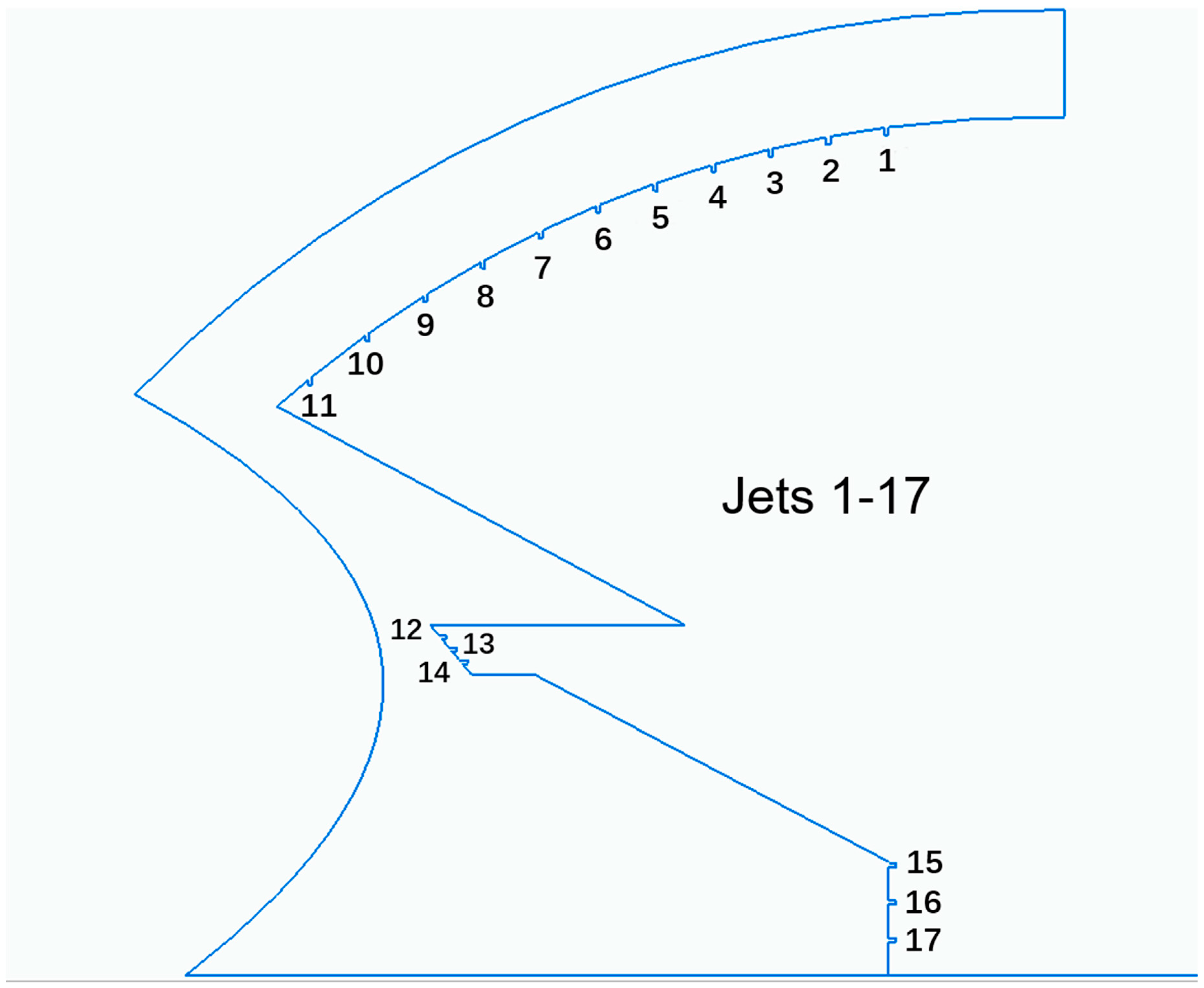
In this section, the developed model of the stadium and surrounding environment is validated by comparing the dimensionless wind velocity magnitude for each gate from the present study with that from a previous work [11]. The modelling method of air curtains is also verified on the basis of previous experimental results [28]. To obtain more realistic thermal boundary conditions for the assessments of cooling configurations and a baseline configuration, separate solar radiation simulations are performed to predict the radiative heat fluxes from the surfaces of the ground, stadium and surrounding buildings. The results are used as thermal boundary conditions for the further assessments. Three cooling configurations are proposed in this research. Configuration 1 and 2 are designed on the basis of a cooling jet configuration proposed by [19], as shown in Figure 5. The difference between the two configurations is that only the vertical jets 1–11 are used to supply cool air under configuration 1, but configuration 2 has all the jets supplying cool air. Configuration 3 is also designed on the foundation of this cooling jet configuration. However, the horizontal jets 15–17 around the pitch are removed and four gates of the stadium are equipped with air curtains. Three scenarios are proposed under each cooling configuration in order to explore the effects of supply velocities of vertical jets above tiers, horizontal jets around the pitch and air curtains at gates on the pitch thermal conditions. The locations, supply air temperatures and velocity magnitudes are presented in Table 3. The thermal and wind conditions of these three configurations are evaluated and compared with the baseline configuration of the stadium without employing any cooling techniques. The thermal comfort levels on the spectator tiers and the pitch are evaluated for each scenario using the ASHRAE method (Standard 55–2017) [20], where the thermal sensation scale is represented by the Predicted Mean Vote (PMV) ranging from +3 hot to 0 neutral and to −3 cold. It should be noted that we did not aim to accurately predict the thermal comfort levels inside the stadium but instead use them as indicators to compare the three cooling configurations and the baseline configuration. The energy consumption per match consumed by each scenario is also estimated as another indicator.
3.1. Stadium and Surrounding Environment Modelling Validation
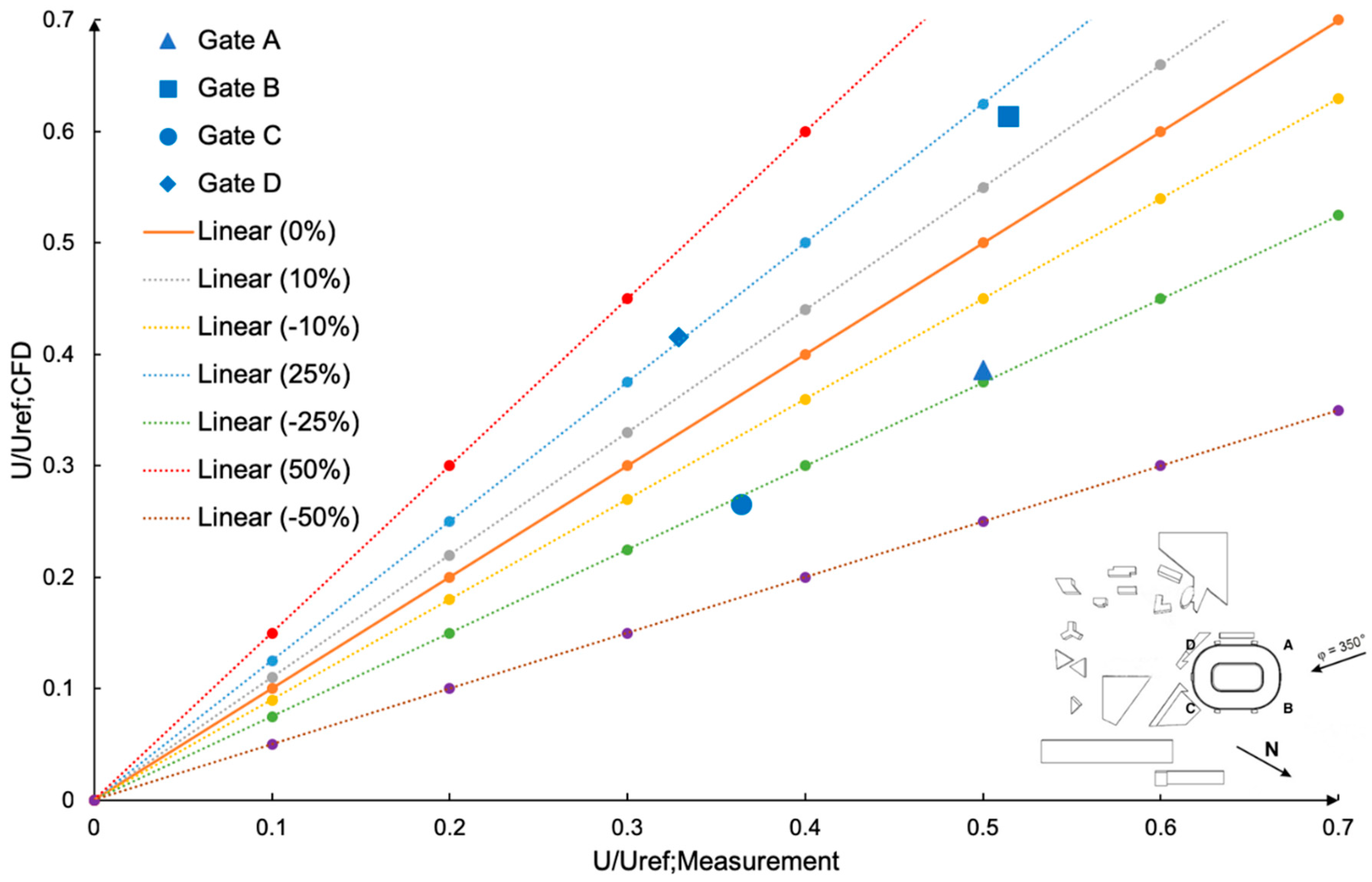
The developed model of the stadium and surrounding buildings was simulated under the wind direction of φ = 350° and the average wind velocity at each gate of the stadium was measured and compared with the previous field measurement data [11]. The dimensionless wind velocity magnitude U/Uref for each gate was calculated on the basis of the current CFD simulation results and the previous field measurements, as shown in Table 4. The average wind velocity at each gate obtained from the two methods and the errors between the two methods are also presented in Table 4. The results of the two methods were also plotted in a graph showing errors between these methods (Figure 6). The deviations between the CFD simulation results and the field measurement data could be explained by that the exact field measurement locations were not given by [11]. A slight deviation between the measured locations from CFD simulations and those from the field testing can lead to a significant difference in the values of wind velocity between the two results. The errors demonstrate a fair to good agreement, and thus the developed model of the stadium and surrounding buildings was validated and used for further simulations.
3.2. Cooling Jets and Air Curtains Modelling Method Validation
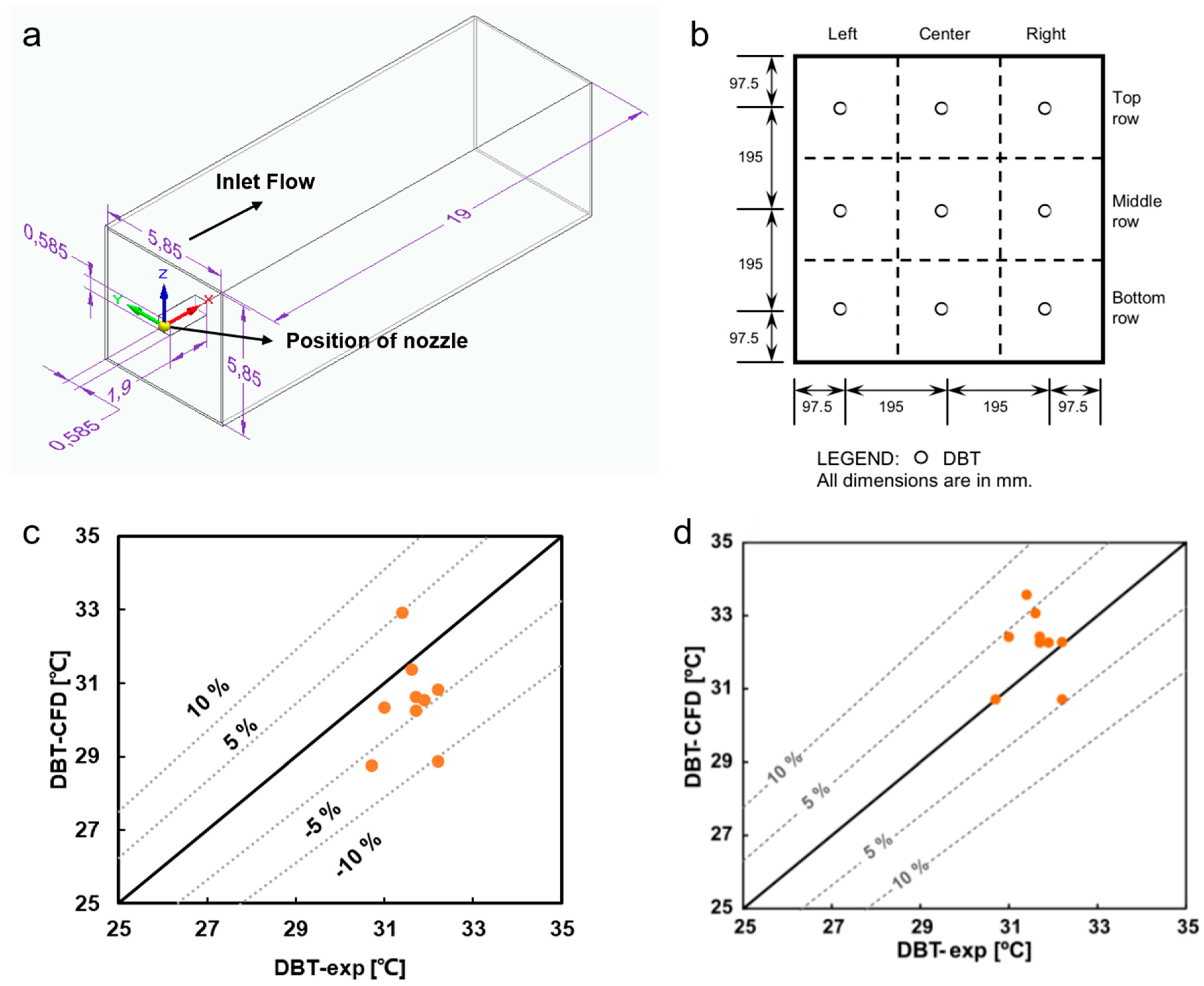
The characteristics of cooling jets were validated on the basis of previous experimental measurements [48] and CFD simulation results [49]. The cooling jet was modelled as a reduced-scale spray nozzle with a diameter of 4 mm in a simplified computational domain of 0.585 m × 0.585 m × 1.9 m (Figure 7a), which was used as the wind tunnel test section in the experiment [48]. The boundary conditions of the domain, the characteristics of the nozzle and the Fluent setup were based on [49] and therefore not repeated in this paper. The dry-bulb temperatures (DBTs) were measured by nine measurement points (at the centre of each 3 × 3 grid) (Figure 7b) on the outlet plane of the domain from current CFD simulation and were compared with the measurements on the same points from the previous experimental testing [48] and CFD simulation results [49]. The error between the current CFD results and the previous experimental measurements on each measurement point is plotted in Figure 7c. It is observed that the maximum absolute error is 10% and the absolute deviations between the two results for most of the points are within 5%. The mean absolute error between the two results is calculated as 4.55%, which shows a good agreement between the current CFD results and previous experimental results. Apart from this, the graph plotting the relationship between the DBTs from the current CFD simulations and the previous experimental testing [48] (Figure 7c) is compared with the graph presenting the relationship between the DBTs from previous CFD simulations [49] and experimental testing [48] (Figure 7d). The maximum absolute error is around 7% and the absolute errors for the remaining points are within 5%, which are close to those from the current study. But the trends of data points are slightly different between the two graphs. The DBTs from current simulations are generally lower than those from previous simulations, which also results in the fact that the DBTs from current simulations are overall lower than those from the previous experimental measurements. These discrepancies maybe caused by the different discrete phase model conditions set for the walls of the domain. The ‘reflected’ boundary condition was used in the previous simulations while the ‘escape’ condition was set in the current simulations, considering the larger domain of the stadium environment than the simplified domain used in the previous simulations. Overall, the validity of the characteristics of the cooling jets were verified.
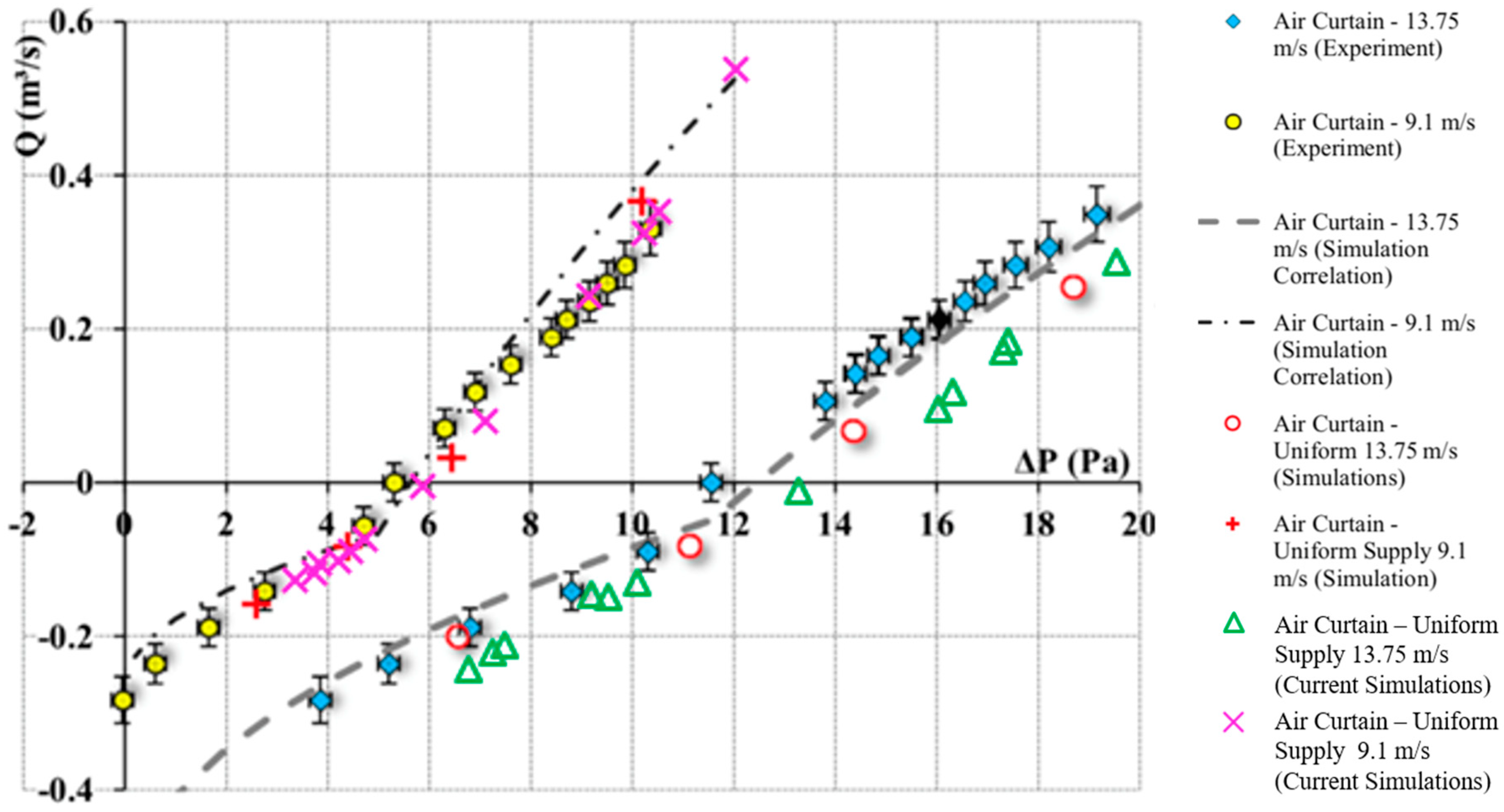
The air curtains used in the present study were modelled as supply slots, according to a previous study [28]. To validate the modelling method of air curtains, a full-scale test chamber, equipped with an air curtain door, a duct blaster fan for adjusting the airflow rate through the door/fan and its surrounding environment was developed and simulated under similar boundary conditions to the experiment setup [28]. The supply slot of the air curtain unit is modelled with a size of 0.0635 m × 0.61 m (Dac × Wac) and the dimensions of the door are 0.61 m × 0.71 m (Wd × Hd). The test chamber size is 2.44 m × 2.44 m × 1.3 m (Lc × Wc × Hc). The air curtain in the present study is simulated under two uniform supply speeds of 13.75 m/s and 9.1 m/s. The boundary conditions and Fluent setup are set similar to those introduced in previous work [27,28,29] and thus are not repeated in this paper. The net airflow rates through the air curtain door Q (m3/s) under various pressure differences across the door ΔP were obtained from the CFD simulations results and compared with previous experimental and numerical results. The results of airflow rates and their corresponding pressure differences from current simulations and previous simulations and experiments are plotted in Figure 8. The simulation correlations of these two variables are also plotted by previous work [28] and illustrated in Figure 8. The green triangular and magenta cross symbols represent the current simulation results under uniform supply speeds of 13.75 m/s and 9.1 m/s. Although the airflow rates from the current results are overall lower than those measured by the experiment and those predicted by the correlations, the general trend of the air curtain flow characteristics is still captured by the current results. It should be noted that the uniform supply speeds, instead of the real supply profiles of the air curtain unit used for testing, which is not provided in the previous study [28], are applied in the validation simulations. This assumption can account for a portion of the discrepancies between the current simulation results and the previous experimental and numerical results. Some data points under the supply speed of 9.1 m/s are even considerably close to the previous experimental results and correlations. Hence, the simplified modelling method of air curtains is valid to be used in the present research.
3.3. Solar Radiation Simulation Results
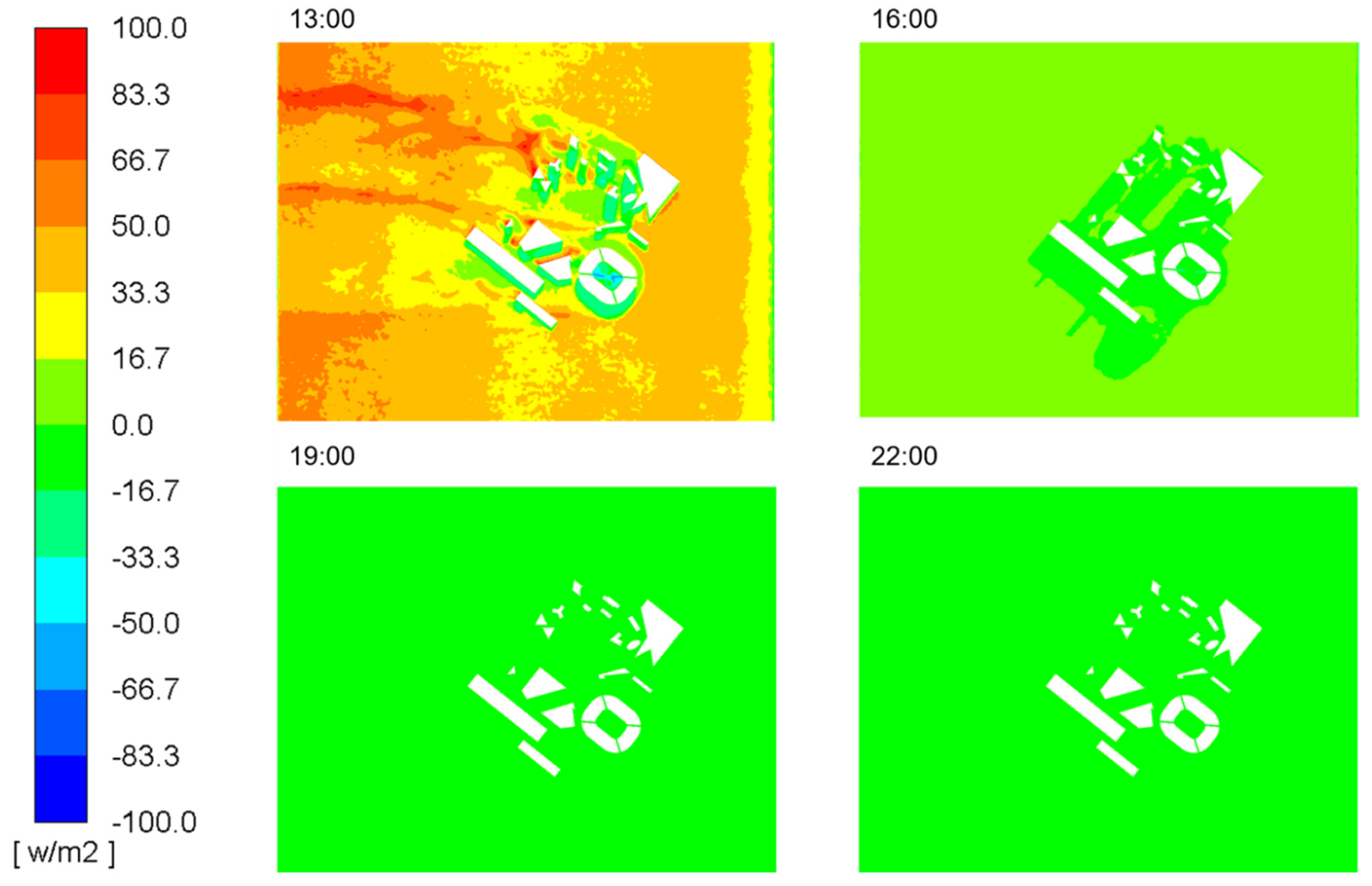
To evaluate the thermal and wind flow conditions inside the stadium under more realistic thermal boundary conditions, de-coupled solar radiation simulations were implemented using the solar irradiance data in Doha under the fair weather conditions method [36] in order to predict radiative heat fluxes emitted from the surfaces of ground, stadium and surrounding buildings. The results were thus used as the thermal boundary conditions for simulations which evaluate the thermal and wind flow conditions inside the stadium. It should be noted that the de-coupled solar radiation simulations were introduced here and conducted due to less computational resources consumed by two separate sets of simulations. It should also be noted that these simulations are not aimed to accurately predict the actual radiative heat fluxes but to minimize the gap between the numerical simulation results and the real thermal and wind flow conditions in the stadium. The effect of solar irradiances on the radiative heat fluxes of these surfaces was assessed under four proposed kick-off times, i.e., 13:00, 16:00, 19:00 and 22:00 GMT+3 (Doha time) on 21 November of the proposed opening day of the World Cup [45]. The corresponding radiative heat fluxes of these surfaces for each kick-off time are presented in Table 5. Besides, the radiative heat flux contours of the ground for each kick-off time are shown in Figure 9. It is obviously observed that the radiative heat fluxes from the ground at 13:00 is the most intensive among those for the four kick-off times. Hence, the results obtained from the solar radiation simulation under 13:00 are used as the thermal boundary conditions for the further assessments of each cooling configuration and a baseline configuration.
3.4. Influence of Vertical Jets Supply Velocity on Pitch Thermal Conditions
Scenarios 1–3 are proposed under configuration 1 which has only the vertical jets above the tiers providing the cooling for the stadium. The influence of different supply air velocities of vertical jets on the thermal conditions of the pitch is assessed. The temperature distributions on the pitch of these scenarios are presented in Figure 10a–c. It is observed that the temperature distributions of the pitch for these scenarios are significantly affected by the hot outside air of 34.2 °C and approximately 5 m/s entering from one of the gates, since the temperatures at one of the corners of the pitch reach 35.0 °C. Scenarios 1–2, which have lower supply air velocities for each jet, experience more heavily the influence of the infiltration of outside air on the pitch thermal distributions than scenario 3. Remarkably, for scenarios 1–2, the hot outside air inflow heats through one of the diagonals of the pitch, resulting in the pitch temperature rising up to at least 28.3 °C. Scenario 3 shows that increasing the jet supply velocity has the potential to attenuate the effect of the outside air inflow heating the pitch but is not effective to cool down the regions being affected by this inflow, where temperatures are still over 28.3 °C. In addition, the remaining pitch is cooled to 20 °C to 25 °C, conforming with the FIFA’s comfort temperature requirement. In terms of thermal comfort for players, the maximum Predicted Percentage of Dissatisfied (PPD) of these scenarios, as shown in Table 6, are in the range of 80% to 95%, which means ‘Warm’ to ‘Hot’ sensations for players [20].
3.5. Influence of Horizontal Jets Supply Velocity on the Pitch Thermal Conditions
To study the influence of supply velocities of horizontal jets around the pitch on the temperature distributions of the pitch, three velocities of 6 m/s, 10 m/s and 12 m/s are used for horizontal jets around the pitch under configuration 2. Similar to scenarios 1–3, the hot outside air infiltration occurs at the same gate of the stadium for scenarios 4–6 (Figure 10d–f). However, the enhancement on the jet supply velocity of horizontal jets around the pitch is effective in reducing the high temperature regions of 28.3 °C to 35.0 °C around that corner of the pitch. Scenario 4 is still largely affected by the outside air inflow, since approximately a quarter of the pitch is heated by this inflow to at least 26.7 °C to 28.3 °C. The areas of regions being influenced by the inflow for scenarios 5–6 are decreased compared with those for scenario 4. Apart from this, the rest of the pitch for these three scenarios show good thermal conditions of 20 °C to 23.3 °C, which satisfy the comfort temperature requirement of FIFA. As for the thermal comfort for players, the players under scenario 4 still sense ‘Warm’ [20] since the PMV and the PPD are still 1.63 and 58%, respectively. However, the comfort is enhanced substantially for scenarios 5–6, which have the PPDs of 29% and 8%, respectively. ‘Slightly warm’ and ‘Neutral’ [20] thermal sensations are provided by scenarios 5–6, respectively, which are fair to good for players’ comfort and health. It should be noted that the thermal comfort levels presented above are intended to represent the overall performances of comfort on the pitch, and therefore those extreme values on the pitch corner areas, which are empirically less used in football games than the central regions of the pitch, are not included in the thermal comfort estimations.
3.6. Influence of Air Curtains Supply Velocity on the Pitch Thermal Conditions
Air curtains are employed in configuration 3 to assess their potential on providing a solution to the issue of local hot regions caused by the infiltration of outside hot air. Three different supply air velocities of 10 m/s, 15 m/s and 20 m/s are used in scenarios 7–9, respectively. The thermal conditions on the pitch for scenarios 7–9 are illustrated in Figure 10g–i. It is observed that the issue caused by the infiltration of outside hot air is solved by the use of air curtains for the three scenarios. The temperature distributions of 20 °C to 26.7 °C are presented by scenario 7 (Figure 10g), where the temperatures of 25.0 °C to 26.7 °C at the central region of the pitch are slightly higher than the upper threshold of the FIFA’s comfort temperatures. The other two scenarios demonstrate good thermal conditions of 20 °C to 25 °C, which are within the comfort temperature range. Moreover, the penetration of the outside hot air into the stadium is sufficiently blocked by the air curtains with supply velocity of 20 m/s for scenario 9. With respect to thermal comfort on the pitch, the PMV and the PPD of the pitch for scenario 9 are reduced to 1.02 and 27%, respectively. But the thermal sensation for players is still ‘Slightly warm’ [20] since the air velocities on the pitch (Figure 11i) are mainly lower than 1.3 m/s. The wind environment on the pitch should be improved in future studies to provide more active air circulations on the pitch.
3.7. Comparison between Cooling Configurations and Baseline Configuration
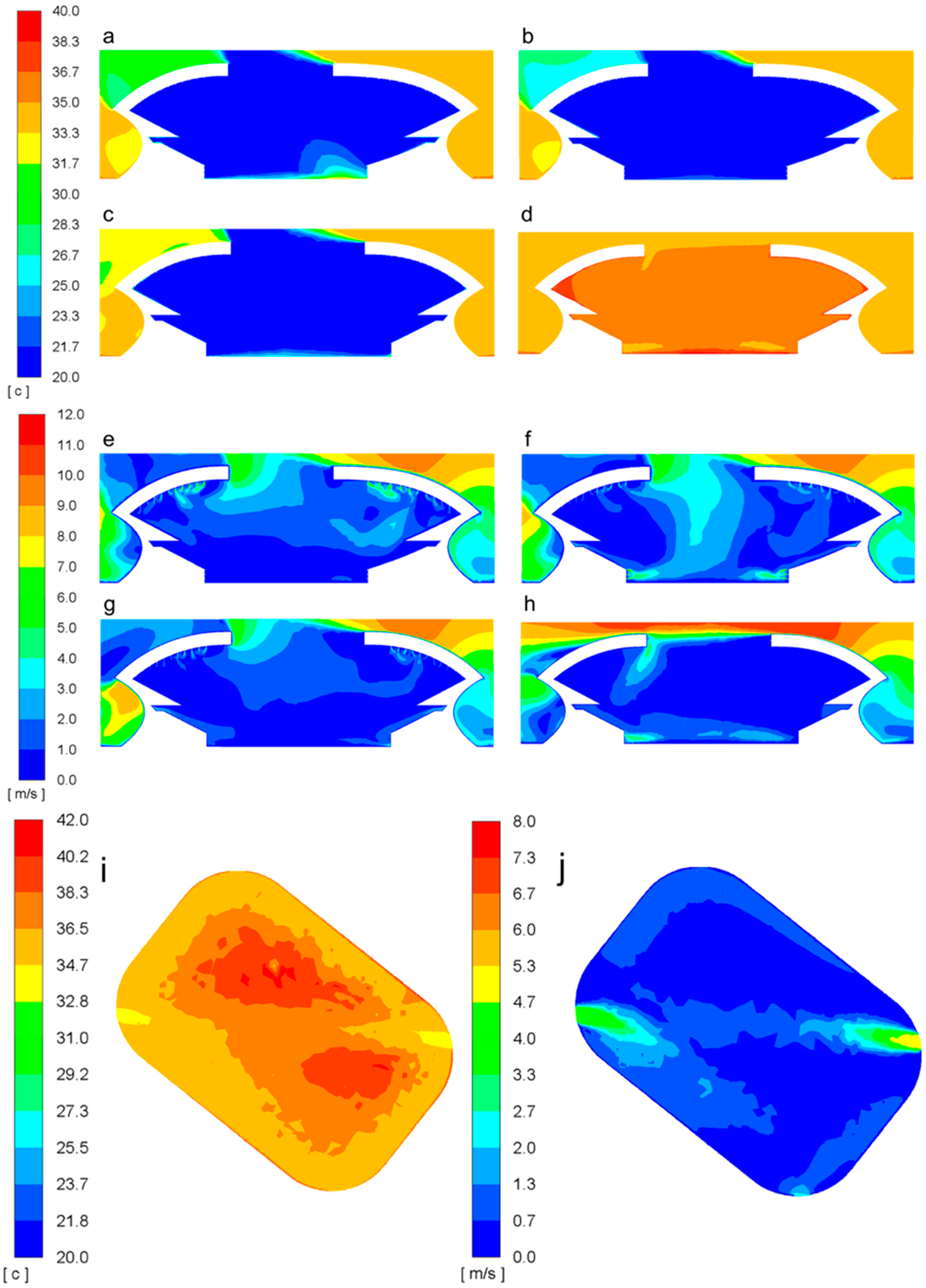
The three cooling configurations of vertical jets only, vertical and horizontal jets, integrated jets and air curtains and the baseline configuration without using any cooling techniques are assessed and compared in order to show their cooling performances for the stadium. One scenario with the highest supply air velocities for jets or air curtains is selected from each cooling configuration and its temperature and wind velocity distributions on the cross section of the stadium are shown in Figure 12a–c,e–g, respectively. The three configurations (Figure 12a–c) can all provide the spectator tiers with comfortable temperatures of 20 °C to 21.7 °C. However, the temperature at the region below the lower spectator tiers for configuration 1 (Figure 12a) rises over 25.0 °C, since this region is heated by the outside hot inflow from one of the gates (Figure 11c). As for the wind conditions, the air circulation at the upper tiers is more active than that at the lower tiers for configuration 1 (Figure 12e), since the cool air is only supplied by vertical jets. In addition to this configuration, the lower tiers have a higher air velocity of 1–2 m/s than that of 0–1 m/s at the upper tiers for configuration 2 and 3 (Figure 12f–g), which both have lower supply air velocities of vertical jets but use horizontal jets at the back of lower tiers. Compared with the baseline configuration, the thermal environment at spectator tiers is all significantly enhanced by these cooing configurations, since the temperature at tiers is reduced by at least 15.0 °C. The wind environment of the baseline configuration is influenced by the scouring effect of the wind flow which enters into the stadium through one edge of the roof opening [50] and has poor air circulations inside the stadium. The cooling configurations, especially configuration 2, provide more active air movements inside the stadium. In terms of thermal comfort for the spectators, the baseline configuration is ‘Hot’ for the spectators, since the PMVs for both the upper and lower tiers are close to 3 [20]. However, the cooling configurations can all provide ‘Slightly cool’ thermal sensations for spectators with the PMVs from 0.91 to 1.42 [20].
As for the pitch, configurations 1 and 2 are both affected by the penetration of outside hot air through one of the gates (Figure 10a–f). It is also observed that increasing the jet velocity of horizontal jets around the pitch cannot effectively attenuate the influence of the outside air inflow. However, configuration 3 demonstrates that the penetration of outside air can be prevented by using air curtains at gates (Figure 10g–i). With regards to wind conditions, configuration 2 shows the most active air movements but may affect the motion of the football during matches, since the highest air velocity can reach 4 m/s (Figure 11f). The penetration of outside air is obviously observed in configuration 1 (Figure 11a–c) and is effectively reduced by configuration 3 (Figure 11g–i). In comparison with the baseline configuration, the temperature is decreased by a minimum of 4.8 °C, 9.8 °C and 15.2 °C for configurations 1–3, respectively, and the outside air inflow of up to 5.3 m/s is blocked by configuration 3. The PMV on the pitch is improved from 5.90, which is extremely hot, to 0.35 and 1.02 for configurations 2 and 3, respectively. Although configuration 2 can provide a ‘Neutral’ sensation for players, the energy consumed by configuration 2 for a match is 76.6 MWh, which is considerably higher than that of 54.0 MWh for configuration 3. Hence, for countries in hot climates such as Qatar, which is required to deliver a carbon-neutral World Cup, the use of air curtains can be regarded as an energy-efficient alternative to the typical use of cooling jets for the stadium. However, further research is still required to be conducted in order to investigate the operation conditions of air curtains for stadiums and analyse the sensitivity of air curtain parameters on its performance. Further work can also focus on optimizing the synchronized operation of the cooling jets and air curtains by designing a control system which can adapt to the indoor requirements and the outdoor conditions.
4. Conclusions and Future Work
The present study aims to assess the thermal and wind environment of a semi-outdoor stadium under three different cooling configurations and a baseline configuration without cooling using Computational Fluid Dynamics (CFD) simulations. The three cooling configurations are: (1) vertical jets only above upper tiers, (2) vertical jets above upper tiers and horizontal jets at the back of lower tiers and around the pitch, and (3) integrated vertical jets above upper tiers, horizontal jets at the back of lower tiers and air curtains at gates. Under each cooling configuration, three different scenarios are proposed to evaluate the effect of supply speeds of vertical jets above the tiers, horizontal jets around the pitch and air curtains at gates on the pitch thermal conditions. A full-size stadium model was developed and validated on the basis of previous studies. The characteristics of cooling jets and air curtains were validated by previous experimental and CFD simulation results. De-coupled solar radiation simulations were implemented using the solar irradiance data in Doha under the fair weather conditions method in ANSYS Fluent in order to predict radiative heat fluxes emitted from the surfaces of the ground, stadium and surrounding buildings. The results were used as thermal boundary conditions for simulations assessing the thermal and wind conditions in the stadium. The approach wind was based on the atmospheric boundary layer (ABL) flow profile. Three-dimensional steady Reynolds-averaged Navier–Stokes (RANS) equations and the realizable k-ε model were used to solve the thermal and wind flow conditions. The thermal comfort levels on the spectator tiers and pitch of the stadium were estimated using the ASHRAE PMV method (Standard 55–2017). The energy consumption per match required by each scenario was also evaluated.
On the basis of the evaluations for the influence of supply speeds for (1) vertical jets above the tiers, (2) horizontal jets around the pitch and (3) air curtains at gates on the pitch thermal conditions, the temperature distributions on the pitch for configurations 1 and 2 are both affected by the infiltration of hot outside air of 34.2 °C and approximately 5 m/s entering from one of the gates. Configuration 3 demonstrates that the issue caused by the infiltration of hot outside air can be solved by the use of air curtains. In particular, the penetration of hot outside air into the stadium can be sufficiently blocked by the air curtains with a supply speed of 20 m/s for scenario 9. However, the lowest value of PPD of 27% under configuration 3 is still higher than that of 8% under configuration 2, since air velocities on the pitch under configuration 3 are lower. The wind environment on the pitch under configuration 3 should be improved to provide more active air movements.
Comparing the cooling configurations with the baseline configuration without cooling, the temperature at spectator tiers is reduced by at least 15.0 °C. The pitch temperature is decreased by a minimum of 4.8 °C, 9.8 °C and 15.2 °C by configurations 1–3, respectively. Consequently, the values of PMV on the pitch is improved from 5.90 (extremely hot) of the baseline to 0.35 and 1.02 of configurations 2 and 3, respectively. However, the energy consumption per match required by configuration 3 is only 54.0 MWh, which is considerably lower than that of 76.6 MWh for configuration 2. Therefore, for countries in hot climates, such as Qatar, which is required to deliver a carbon-neutral World Cup, the use of air curtains can be regarded as an energy-efficient alternative to the typical use of cooling jets for stadiums.
Further research is still required to be conducted in order to investigate the operation conditions of air curtains for stadiums and analyse the influence of air curtain parameters on its performance. The wind environment needs to be improved by applying other ventilation techniques in future studies. The sensitivity of supply air temperature and supply angle of air curtains on the pitch thermal conditions is not considered in this study and can be focused on in future. Further study can also focus on optimizing the synchronized operation of the cooling jets and air curtains by designing a control system which can adapt to the indoor requirements and the outdoor conditions.
Author Contributions
Conceptualization, F.Z. and J.C.; methodology, F.Z. and J.C.; software, F.Z.; validation, F.Z.; formal analysis, F.Z.; investigation, F.Z.; resources, J.C.; writing—original draft preparation, F.Z.; writing—review and editing, J.C.; visualization, F.Z.; supervision, J.C.; project administration, J.C.; funding acquisition, J.C. All authors have read and agreed to the published version of the manuscript.
Funding
This research received no external funding.
Acknowledgments
The authors would like to thank the support of the Department of Architecture and Built Environment for providing the facility for conducting the modelling and simulations.
Conflicts of Interest
The authors declare no conflict of interest.
References
- Talavera, A.M.; Al-Ghamdi, S.G.; Koç, M. Sustainability in mega-events: Beyond Qatar 2022. Sustainability 2019, 11, 6407. [Google Scholar] [CrossRef] [Green Version]
- FIFA.com. Available online: https://www.fifa.com/mm/document/afsocial/environment/01/57/12/66/2006fwcgreengoallegacyreport_en.pdf (accessed on 26 November 2018).
- Saffouri, F.; Bayram, I.S.; Koç, M. Quantifying the cost of cooling in Qatar. In Proceedings of the 9th IEEE-GCC Conference and Exhibition, Manama, Bahrain, 8–11 May 2017. [Google Scholar]
- FIFA.com. Available online: https://www.fifa.com/mm/document/tournament/competition/01/37/17/76/stadiumbook2010_buch.pdf (accessed on 26 November 2018).
- FIFA.com. Available online: https://www.fifa.com/worldcup/news/2022-fifa-world-cup-to-be-played-in-november-december-2568172 (accessed on 26 November 2018).
- The American Society of Heating, Refrigeration and Air-conditioning Engineers (ASHRAE). ASHRAE Weather Data 2017; ASHRAE: Atlanta, GA, USA, 2017; p. 929. [Google Scholar]
- Boero, A.; Agyenim, F. Modeling and simulation of a small-scale solar-powered absorption cooling system in three cities with a tropical climate. Int. J. Low-Carbon Technol. 2020, 15, 1–16. [Google Scholar] [CrossRef]
- Sekhar, C.; Anand, P.; Schiavon, S.; Tham, K.W.; Cheong, D.; Saber, E.M. Adaptable cooling coil performance during part loads in the tropics—A computational evaluation. Energy Build. 2018, 159, 148–163. [Google Scholar] [CrossRef]
- Anand, P.; Cheong, D.; Sekhar, C. Computation of zone-level ventilation requirement based on actual occupancy, plug and lighting load information. Indoor Built Environ. 2020, 29, 558–574. [Google Scholar] [CrossRef]
- Irshad, K.; Habib, K.; Basrawi, F.; Saha, B.B. Study of a thermoelectric air duct system assisted by photovoltaic wall for space cooling in tropical climate. J. Energy 2017, 119, 504–522. [Google Scholar] [CrossRef]
- Van Hooff, T.; Blocken, B. Coupled urban wind flow and indoor natural ventilation modelling on a high-resolution grid: A case study for the Amsterdam Arena Stadium. Environ. Model. Softw. 2010, 25, 51–65. [Google Scholar] [CrossRef]
- Van Hooff, T.; Blocken, B. On the effect of wind direction and urban surroundings on natural ventilation of a large semi-enclosed stadium. Comput. Fluids 2010, 39, 1146–1155. [Google Scholar] [CrossRef]
- Van Hooff, T.; Blocken, B. Full-scale measurements of indoor environmental conditions and natural ventilation in a large semi-enclosed stadium: Possibilities and limitations for CFD validation. J. Wind Eng. Ind. Aerodyn. 2012, 104, 330–341. [Google Scholar] [CrossRef]
- Sofotasiou, P. Aerodynamic Optimization of Sports Stadiums towards Wind Comfort. Ph.D. Thesis, University of Sheffield, Sheffield, UK, January 2017. Available online: http://etheses.whiterose.ac.uk/id/eprint/17820 (accessed on 20 October 2018).
- Sofotasiou, P.; Hughes, B.R.; Calautit, J.K. Qatar 2022: Facing the FIFA World Cup climatic and legacy challenges. Sustain. Cities Soc. 2015, 14, 16–30. [Google Scholar] [CrossRef]
- Sofotasiou, P.; Hughes, B.R.; Calautit, J.K. Thermal performance evaluation of semi-outdoor sport stadia: A case study of the upcoming 2022 FIFA World Cup in Qatar. In Proceedings of the ASHRAE Hellenic Chapter, 3rd International Conference “Energy in Buildings 2014”, Athens, Greece, 15 November 2014. [Google Scholar]
- Ghani, S.; ElBialy, E.A.; Bakochristou, F.; Gamaledin, S.M.A.; Rashwan, M.M.; Hughes, B. Thermal performance of stadium’s Field of Play in hot climates. Energy Build. 2017, 139, 702–718. [Google Scholar] [CrossRef]
- Khalil, E.E.; Ashmawy, M.E. The challenge of cooling football stadiums in Qatar. CIBSE J. 2017. Available online: https://www.cibsejournal.com/technical/sporting-success-a-study-of-air-conditioning-stadiums-in-qatar/ (accessed on 17 March 2019).
- Zhong, F.; Calautit, J.K.; Hughes, B.R. Analysis of the influence of cooling jets on the wind and thermal environment in football stadiums in hot climates. Build. Serv. Eng. Res. Technol. 2019, 1–25. [Google Scholar] [CrossRef]
- The American Society of Heating, Refrigeration and Air-conditioning Engineers (ASHRAE). 2017 ASHRAE Handbook Fundamentals; ASHRAE: Atlanta, GA, USA, 2017. [Google Scholar]
- Luo, N.; Li, A.; Gao, R.; Zhang, W.; Tian, Z. An experiment and simulation of smoke confinement utilizing an air curtain. Saf. Sci. 2013, 59, 10–18. [Google Scholar] [CrossRef]
- Giráldez, H.; Pérez Segarra, C.D.; Oliet, C.; Oliva, A. Heat and moisture insulation by means of air curtains: Application to refrigerated chambers. Int. J. Refrig. 2016, 68, 1–14. [Google Scholar] [CrossRef] [Green Version]
- Foster, A.M.; Swain, M.J.; Barrett, R.; D’Agaro, P.; Ketteringham, L.P.; James, S.J. Three-dimensional effects of an air curtain used to restrict cold room infiltration. Appl. Math. Model. 2007, 31, 1109–1123. [Google Scholar] [CrossRef]
- Lecaros, M.; Elicer-Cortés, J.C.; Fuentes, A.; Felis, F. On the ability of twin jets air curtains to confine heat and mass inside tunnels. Int. Commun. Heat Mass Transf. 2010, 37, 970–977. [Google Scholar] [CrossRef]
- Wang, B.; Yu, J.; Ye, H.; Liu, Y.; Guo, H.; Tian, L. Study on present situation and optimization strategy of infiltration air in a train station in winter. Procedia Eng. 2017, 205, 2517–2523. [Google Scholar] [CrossRef]
- Hayes, F.C.; Stoecker, W.F. Design data for air curtains. Trans. ASHRAE 1969, 75, 168–180. [Google Scholar]
- Wang, L.; Zhong, Z. An approach to determine infiltration characteristics of building entrance equipped with air curtains. Energy Build. 2014, 75, 312–320. [Google Scholar] [CrossRef]
- Goubran, S.; Qi, D.; Saleh, W.F.; Wang, L.; Zmeureanu, R. Experimental study on the flow characteristics of air curtains at building entrances. Build. Environ. 2016, 105, 225–235. [Google Scholar] [CrossRef]
- Qi, D.; Goubran, S.; Wang, L.; Zmeureanu, R. Parametric study of air curtain door aerodynamics performance based on experiments and numerical simulations. Build. Environ. 2018, 129, 65–73. [Google Scholar] [CrossRef] [Green Version]
- Blocken, B.; Persoon, J. Pedestrian wind comfort around a large football stadium in an urban environment: CFD simulation, validation and application of the new Dutch wind nuisance standard. J. Wind Eng. Ind. Aerodyn. 2009, 97, 255–270. [Google Scholar] [CrossRef]
- Franke, J.; Hellsten, A.; Schlünzen, H.; Carissimo, B. Best Practice Guideline for the CFD Simulation of Flows in the Urban Environment; COST Office: Brussels, Belgium, 2007; pp. 16–18. Available online: https://www.semanticscholar.org/paper/BEST-PRACTICE-GUIDELINE-FOR-THE-CFD-SIMULATION-OF-Franke-Hellsten/bc39516aba1e74f7d8ed7391b4ff9e5a9ceeecf2 (accessed on 2 May 2019).
- Bartzis, J.G.; Vlachogiannis, D.; Sfetsos, A. Thematic area 5: Best practice advice for environmental flows. QNET-CFD Netw. Newsl. 2004, 2, 34–39. [Google Scholar]
- Cowan, I.R.; Castro, I.P.; Robins, A.G. Numerical considerations for simulations of flow and dispersion around buildings. J. Wind Eng. Ind. Aerodyn. 1997, 67, 535–545. [Google Scholar] [CrossRef]
- Blocken, B.; Stathopoulos, T.; Carmeliet, J. CFD simulation of the atmospheric boundary layer: Wall function problems. Atmos. Environ. 2007, 41, 238–252. [Google Scholar] [CrossRef]
- Casey, M.; Wintergerste, T. Quality and Trust in Industrial CFD, 1st ed.; European Research Community on Flow, Turbulence and Combustion: Brussels, Belgium, 2000. [Google Scholar]
- ANSYS, Inc. Fluent User’s Guide 18.2; ANSYS, Inc.: Canonsburg, PA, USA, 2017. [Google Scholar]
- Weather Online. Available online: https://www.weatheronline.co.uk/weather/maps/city (accessed on 18 March 2019).
- Blumberg, D.G.; Greeley, R. Field studies of aerodynamic roughness length. J. Arid Environ. 1993, 25, 39–48. [Google Scholar] [CrossRef]
- Launder, B.E.; Spalding, D.B. The numerical computation of turbulent flows. Comput. Methods Appl. Mech. Eng. 1974, 3, 269–289. [Google Scholar] [CrossRef]
- Cebeci, T.; Bradshaw, P. Momentum Transfer in Boundary Layers; Hemisphere Publ. Co.: Washington, DC, USA, 1977. [Google Scholar]
- Incropera, F.P. Introduction to Heat Transfer, 5th ed.; John Wiley & Sons: Franklin Township, NJ, USA, 2007. [Google Scholar]
- Shih, T.H.; Liou, W.W.; Shabbir, A.; Yang, Z.; Zhu, J. A new k-ε eddy viscosity model for high Reynolds number turbulent flows. Comput. Fluids 1995, 24, 227–238. [Google Scholar] [CrossRef]
- Mochida, A.; Tominaga, Y.; Murakami, S.; Yoshie, R.; Ishihara, T.; Ooka, R. Comparison of various k-ε models and DSM to flow around a high-rise building—Report of AIJ cooperative project for CFD prediction of wind environment. Wind Struct. 2002, 5, 227–244. [Google Scholar] [CrossRef] [Green Version]
- Franke, J.; Hirsch, C.; Jensen, A.G.; Krüs, H.W.; Schatzmann, M.; Westbury, P.S.; Miles, S.D.; Wisse, J.A.; Wright, N.G. Recommendations on the use of CFD in wind engineering. In Proceedings of the COST Action C14, Rhode-Saint-Genèse, Belgium, 5–7 May 2004; Available online: https://www.researchgate.net/profile/Carlo_Gualtieri/post/is_it_irrational_to_validate_a_system_of_equations_for_CFD_with_one_data/attachment/59d6467ec49f478072eae72e/AS%3A273834991652864%401442298757032/download/Franke_2004.pdf (accessed on 2 May 2019).
- Kick-off Times Confirmed for 2022 FIFA World Cup in Qatar. Available online: https://punditarena.com/football/mcorry/kick-off-qatar-world-cup-fifa/ (accessed on 12 January 2020).
- Perez-Astudillo, D.; Bachour, D. DNI, GHI and DHI ground measurements in Doha, Qatar. Energy Procedia 2014, 49, 2398–2404. [Google Scholar] [CrossRef] [Green Version]
- Integrated Environmental Solutions, Inc. Apachesim calculation methods Virtual Environment 6.3; Integrated Environmental Solutions, Inc.: Glasgow, Scotland.
- Sureshkumar, R.; Kale, S.R.; Dhar, P.L. Heat and mass transfer processes between a water spray and ambient air–I. Experimental data. Appl. Therm. Eng. 2008, 28, 349–360. [Google Scholar] [CrossRef]
- Montazeri, H.; Blocken, B.; Hensen, J.L.M. Evaporative cooling by water spray systems: CFD simulation, experimental validation and sensitivity analysis. Build. Environ. 2015, 83, 129–141. [Google Scholar] [CrossRef]
- Simpson, M. Computerised Design of Stadiums. In Stadium and Arena Design, 2nd ed.; Culley, P., Pascoe, J., Eds.; Institution of Civil Engineers (ICE): London, UK, 2015; pp. 119–132. [Google Scholar]
Figure 1.
(a) The Johan Cruyff Arena and its surrounding buildings situated in a radius of 300 m from the stadium from a previous work [30]. (b) Geometry model of the stadium and its surrounding buildings used in the present study. (c) Extension dimensions and boundary conditions of the computational domain (section view). (d) Extension dimensions and boundary conditions of the computational domain (top view).

Figure 2.
The case study stadium Johan Cruyff Arena. (a) Horizontal cross-section at a height of 2 m above the ArenA deck. (b) Vertical cross-section αα’. (c) Vertical cross-section ββ’. (d) Vertical cross-section of the eastern part of the stadium. (e) External view of the stadium with the open roof [11,13].

Figure 3.
(a) Measurement points on the cross-section of the stadium for the grid independence study. (b) Measurement points on the pitch for the grid independence study.
Figure 3.
(a) Measurement points on the cross-section of the stadium for the grid independence study. (b) Measurement points on the pitch for the grid independence study.

Figure 4.
(a) Wind direction frequency for November and December in recent five years. (b) The winter prevailing wind direction used in the simulations (modified from [11]). (c) Inlet wind profiles of mean wind velocity U, turbulence kinetic energy k and turbulence dissipation rate for m and m [12].

Figure 5.
The cooling jets configuration used for cooling configurations 1 and 2.

Figure 6.
Comparison between current Computational Fluid Dynamics (CFD) results and previous field measurements under the wind direction of 350°.
Figure 6.
Comparison between current Computational Fluid Dynamics (CFD) results and previous field measurements under the wind direction of 350°.

Figure 7.
(a) The computational domain of the jet model from the present study. (b) The locations of dry-bulb temperature (DBT) measurement points on the outlet plane (modified from [48]). (c) DBTs comparison between current CFD results and previous experimental measurements [48]. (d) DBTs comparison between previous CFD results [49] and previous experimental measurements [48].

Figure 8.
Comparisons among the current CFD results Q-ΔP for the air curtain with uniform supply and the previous experimental and numerical results [28].
Figure 8.
Comparisons among the current CFD results Q-ΔP for the air curtain with uniform supply and the previous experimental and numerical results [28].

Figure 9.
Radiation heat flux contours of the ground for the kick-off times 13:00, 16:00, 19:00 and 22:00 GMT+3 (Doha time) on 21 November.
Figure 9.
Radiation heat flux contours of the ground for the kick-off times 13:00, 16:00, 19:00 and 22:00 GMT+3 (Doha time) on 21 November.

Figure 10.
(a–i) Temperature distributions of the pitch (at height of 2.1 m) for scenarios 1–9.

Figure 11.
(a–i) Wind velocity magnitude distributions of the pitch (at a height of 2.1 m) for scenarios 1–9.
Figure 11.
(a–i) Wind velocity magnitude distributions of the pitch (at a height of 2.1 m) for scenarios 1–9.

Figure 12.
(a–d) Temperature distributions of the cross-section of the stadium for configurations 1–3 and the baseline configuration. (e–h) Wind velocity distributions of the cross-section of the stadium for configurations 1–3 and the baseline configuration. (i) Temperature distributions of the pitch for the baseline configuration. (j) Wind velocity distributions of the pitch for the baseline configuration.


Table 1.
Boundary conditions for the Computational Fluid Dynamics (CFD) models.
| CFD Boundary Conditions | |
|---|---|
| Domain inlet | Velocity-inlet with a wind profile of y0 = 1 m; inflow temperature of 34.2 °C. |
| Domain Outlet | Pressure-outlet with gauge pressure of 0 Pa; backflow temperature of 34.2 °C. |
| Ground (wall) | ks = 0.59 m Cs = 0.5; heat flux of 36.40 W/m2; material is set up as soil (ρ = 1400 kg/m3; Cp = 1480 J/kgK; k = 0.75 W/mK) [41] |
| Stadium (wall) | ks = 0 m Cs = 0.5; heat flux of 11.25 W/m2; material is set up as concrete (ρ = 2400 kg/m3; Cp = 880 J/kgK; k = 0.3 W/mK) [41] |
| Surrounding buildings (wall) | ks = 0 m Cs = 0.5; heat flux of 3.10 W/m2; material is set up as concrete (ρ = 2400 kg/m3; Cp = 880 J/kgK; k = 0.3 W/mK) [41] |
| Air curtains/Cooling jets | Velocity-inlets with constant velocity magnitudes and temperatures [15,24]. |
Table 2.
Fluent simulation setup.
| Fluent Simulation Setup | |
|---|---|
| Simulation condition | Steady state |
| Turbulence model | Realizable k-ε model with standard wall functions and full buoyancy effect |
| Radiation model 1 | Discrete ordinates (DO) model |
| Solar load model | Solar ray tracing model |
| Solar calculator | |
| Longitude and latitude | 51.53° E 25.29° N |
| Timezone (±GMT) | GMT +3 |
| Date and time | November 21st 13:00, 16:00, 19:00 and 22:00 (GMT +3) |
| Solar irradiation method | Fair weather conditions |
| Sunshine factor | 0.3 |
| Solution method | Pressure-velocity coupling |
| Scheme | SIMPLE |
| Spatial discretization | Second-order discretization schemes |
| Under-relaxation factors | Default values |
| Convergence Criteria | None (Continuity, x, y, z velocities, energy, turbulent kinetic energy k and turbulent dissipation rate ε are monitored) |
1 Note that the radiation model was only adopted in the solar radiation simulations.
Table 3.
Cooling scenarios under each cooling configuration.
| Cooling Configuration 1 | |||
|---|---|---|---|
| Scenario 1 | Location | Supply velocity (m/s) | Supply temperature () |
| Jets 1–5 | Above upper tiers | 6 | 20 |
| Jets 6–8 | Above upper tiers | 3 | 20 |
| Jets 9–10 | Above upper tiers | 2 | 20 |
| Jets 11 | Above upper tiers | 1 | 20 |
| Scenario 2 | Location | Supply velocity (m/s) | Supply temperature () |
| Jets 1–5 | Above upper tiers | 8 | 20 |
| Jets 6–8 | Above upper tiers | 4 | 20 |
| Jets 9–10 | Above upper tiers | 2 | 20 |
| Jets 11 | Above upper tiers | 1 | 20 |
| Scenario 3 | Location | Supply velocity (m/s) | Supply temperature () |
| Jets 1–5 | Above upper tiers | 12 | 20 |
| Jets 6–8 | Above upper tiers | 6 | 20 |
| Jets 9–10 | Above upper tiers | 4 | 20 |
| Jets 11 | Above upper tiers | 2 | 20 |
| Cooling configuration 2 | |||
| Scenario 4 | Location | Supply velocity (m/s) | Supply temperature () |
| Jets 1–5 | Above upper tiers | 6 | 20 |
| Jets 6–8 | Above upper tiers | 3 | 20 |
| Jets 9–10 | Above upper tiers | 2 | 20 |
| Jets 11 | Above upper tiers | 1 | 20 |
| Jets 12–14 | At the back of lower tiers | 4 | 20 |
| Jets 15–17 | Around the pitch zone | 6 | 20 |
| Scenario 5 | Location | Supply velocity (m/s) | Supply temperature () |
| Jets 1–5 | Above upper tiers | 6 | 20 |
| Jets 6–8 | Above upper tiers | 3 | 20 |
| Jets 9–10 | Above upper tiers | 2 | 20 |
| Jets 11 | Above upper tiers | 1 | 20 |
| Jets 12–14 | At the back of lower tiers | 4 | 20 |
| Jets 15–17 | Around the pitch zone | 10 | 20 |
| Scenario 6 | Location | Supply velocity (m/s) | Supply temperature () |
| Jets 1–5 | Above upper tiers | 6 | 20 |
| Jets 6–8 | Above upper tiers | 3 | 20 |
| Jets 9–10 | Above upper tiers | 2 | 20 |
| Jets 11 | Above upper tiers | 1 | 20 |
| Jets 12–14 | At the back of lower tiers | 4 | 20 |
| Jets 15–17 | Around the pitch zone | 12 | 20 |
| Cooling configuration 3 | |||
| Scenario 7 | Location | Supply velocity (m/s) | Supply temperature () |
| Jets 1–5 | Above upper tiers | 6 | 20 |
| Jets 6–8 | Above upper tiers | 3 | 20 |
| Jets 9–10 | Above upper tiers | 2 | 20 |
| Jets 11 | Above upper tiers | 1 | 20 |
| Jets 12–14 | At the back of lower tiers | 4 | 20 |
| Air curtain 1 | Gate A | 10 | 20 |
| Air curtain 2 | Gate B | 10 | 20 |
| Air curtain 3 | Gate C | 10 | 20 |
| Air curtain 4 | Gate D | 10 | 20 |
| Scenario 8 | Location | Supply velocity (m/s) | Supply temperature () |
| Jets 1–5 | Above upper tiers | 6 | 20 |
| Jets 6–8 | Above upper tiers | 3 | 20 |
| Jets 9–10 | Above upper tiers | 2 | 20 |
| Jets 11 | Above upper tiers | 1 | 20 |
| Jets 12–14 | At the back of lower tiers | 4 | 20 |
| Air curtain 1 | Gate A | 15 | 20 |
| Air curtain 2 | Gate B | 15 | 20 |
| Air curtain 3 | Gate C | 15 | 20 |
| Air curtain 4 | Gate D | 15 | 20 |
| Scenario 9 | Location | Supply velocity (m/s) | Supply temperature () |
| Jets 1–5 | Above upper tiers | 6 | 20 |
| Jets 6–8 | Above upper tiers | 3 | 20 |
| Jets 9–10 | Above upper tiers | 2 | 20 |
| Jets 11 | Above upper tiers | 1 | 20 |
| Jets 12–14 | At the back of lower tiers | 4 | 20 |
| Air curtain 1 | Gate A | 20 | 20 |
| Air curtain 2 | Gate B | 20 | 20 |
| Air curtain 3 | Gate C | 20 | 20 |
| Air curtain 4 | Gate D | 20 | 20 |
Table 4.
CFD wind velocity validation results under the wind direction of 350°.
| Opening | CFD Mean Velocity UCFD (m/s) | UCFD/Uref 1 | Experimental Mean Velocity Uexp (m/s) | Uexp/Uref 1 | Error |
|---|---|---|---|---|---|
| Gate A | 3.09 | 0.39 | 4.00 | 0.50 | −0.23 |
| Gate B | 4.91 | 0.61 | 4.11 | 0.51 | 0.19 |
| Gate C | 2.13 | 0.27 | 2.91 | 0.36 | −0.27 |
| Gate D | 3.32 | 0.42 | 2.63 | 0.33 | 0.26 |
1 The reference wind velocity Uref used in the study is 8 m/s.
Table 5.
Radiative heat fluxes for ground, stadium and surroundings for each kick-off time on 21 November.
Table 5.
Radiative heat fluxes for ground, stadium and surroundings for each kick-off time on 21 November.
| Radiative Heat Flux | 13:00 | 16:00 | 19:00 | 22:00 |
|---|---|---|---|---|
| Ground (W/m2) | 36.40 | 3.99 | −0.42 | −0.42 |
| Stadium (W/m2) | 11.25 | 9.52 | 7.23 | 7.23 |
| Surrounding (W/m2) | 3.10 | 4.91 | 2.95 | 2.95 |
Table 6.
Thermal comfort levels and estimated energy consumption per match for each scenario.
| Cooling Jet Scenario | Thermal Comfort Estimation (PMV/PPD) | Energy Consumption per Match (MWh) | ||
|---|---|---|---|---|
| Upper Tiers | Lower Tiers | Pitch | ||
| Scenario 1 | −0.91/22% | −0.16/6% | 2.55/94% | 39.6 |
| Scenario 2 | −1.23/37% | −0.54/11% | 2.36/90% | 50.9 |
| Scenario 3 | −1.23/37% | −0.91/22% | 2.10/81% | 79.1 |
| Scenario 4 | −0.91/22% | −1.23/37% | 1.63/58% | 64.7 |
| Scenario 5 | −0.91/22% | −1.23/37% | 1.06/29% | 72.7 |
| Scenario 6 | −0.91/22% | −1.23/37% | 0.35/8% | 76.6 |
| Scenario 7 | −0.91/22% | −1.42/47% | 1.40/46% | 53.6 |
| Scenario 8 | −0.91/22% | −1.42/47% | 1.23/37% | 53.8 |
| Scenario 9 | −0.91/22% | −1.42/47% | 1.02/27% | 54.0 |
© 2020 by the authors. Licensee MDPI, Basel, Switzerland. This article is an open access article distributed under the terms and conditions of the Creative Commons Attribution (CC BY) license (http://creativecommons.org/licenses/by/4.0/).
Share and Cite
MDPI and ACS Style
Zhong, F.; Calautit, J. An Integrated Cooling Jet and Air Curtain System for Stadiums in Hot Climates. Atmosphere 2020, 11, 546. https://doi.org/10.3390/atmos11050546
AMA Style
Zhong F, Calautit J. An Integrated Cooling Jet and Air Curtain System for Stadiums in Hot Climates. Atmosphere. 2020; 11(5):546. https://doi.org/10.3390/atmos11050546
Chicago/Turabian StyleZhong, Fangliang, and John Calautit. 2020. "An Integrated Cooling Jet and Air Curtain System for Stadiums in Hot Climates" Atmosphere 11, no. 5: 546. https://doi.org/10.3390/atmos11050546
Note that from the first issue of 2016, this journal uses article numbers instead of page numbers. See further details here.