Modeling Compact Intracloud Discharge (CID) as a Streamer Burst


1
Department of Engineering Sciences, Uppsala University, 752 37 Uppsala, Sweden
2
Department of Neurophysiology, Karolinska Institute, 171 77 Stockholm, Sweden
3
HEIG-VD, University of Applied Sciences and Arts Western Switzerland, 1401 Yverdon-les-Bains, Switzerland
4
Electromagnetic Compatibility Laboratory, Swiss Federal Institute of Technology (EPFL), 1015 Lausanne, Switzerland
*
Author to whom correspondence should be addressed.
Atmosphere 2020, 11(5), 549; https://doi.org/10.3390/atmos11050549
Submission received: 18 March 2020
/
Revised: 6 May 2020
/
Accepted: 12 May 2020
/
Published: 25 May 2020
(This article belongs to the Section Meteorology)
Abstract
:Narrow Bipolar Pulses are generated by bursts of electrical activity in the cloud and these are referred to as Compact Intracloud Discharges (CID) or Narrow Bipolar Events in the current literature. These discharges usually occur in isolation without much electrical activity before or after the event, but sometimes they are observed to initiate lightning flashes. In this paper, we have studied the features of CIDs assuming that they consist of streamer bursts without any conducting channels. A typical CID may contain about 109 streamer heads during the time of its maximum growth. A CID consists of a current front of several nanosecond duration that travels forward with the speed of the streamers. The amplitude of this current front increases initially during the streamer growth and decays subsequently as the streamer burst continues to propagate. Depending on the conductivity of the streamer channels, there could be a low-level current flow behind this current front which transports negative charge towards the streamer origin. The features of the current associated with the CID are very different from those of the radiation field that it generates. The duration of the radiation field of a CID is about 10–20 μs, whereas the duration of the propagating current pulse associated with the CID is no more than a few nanoseconds in duration. The peak current of a CID is the result of a multitude of small currents associated with a large number of streamers and, if all the forward moving streamer heads are located on a single horizontal plane, the cumulative current that radiates at its peak value could be about 108 A. On the other hand, the current associated with an individual streamer is no more than a few hundreds of mA. However, if the location of the forward moving streamer heads are spread in a vertical direction, the peak current can be reduced considerably. Moreover, this large current is spread over an area of several tens to several hundreds of square meters. The study shows that the streamer model of the CID could explain the fine structure of the radiation fields present both in the electric field and electric field time derivative.
1. Introduction
Narrow Bipolar Pulses or NBP, a type of radiation field generated by electrical activity in the cloud, were discovered first by LeVine [1]. He found that these radiation fields are associated with very high bursts of HF (High Frequency) and VHF (Very High Frequency) radiation. Further analyses of these pulses in thunderstorms in Florida were reported in [2,3,4,5,6,7,8]. Cooray and Lundquist [9] detected them for the first time in tropical storms in Sri Lanka and, more recently, detailed analyses of these pulses in tropical Sri Lanka and Malaysia were conducted by Sharma et al. [10], Gunasekara et al. [11], and Ahmad et al. [12]. The latitude dependence of NBP was investigated by Ahmad et al. [13].
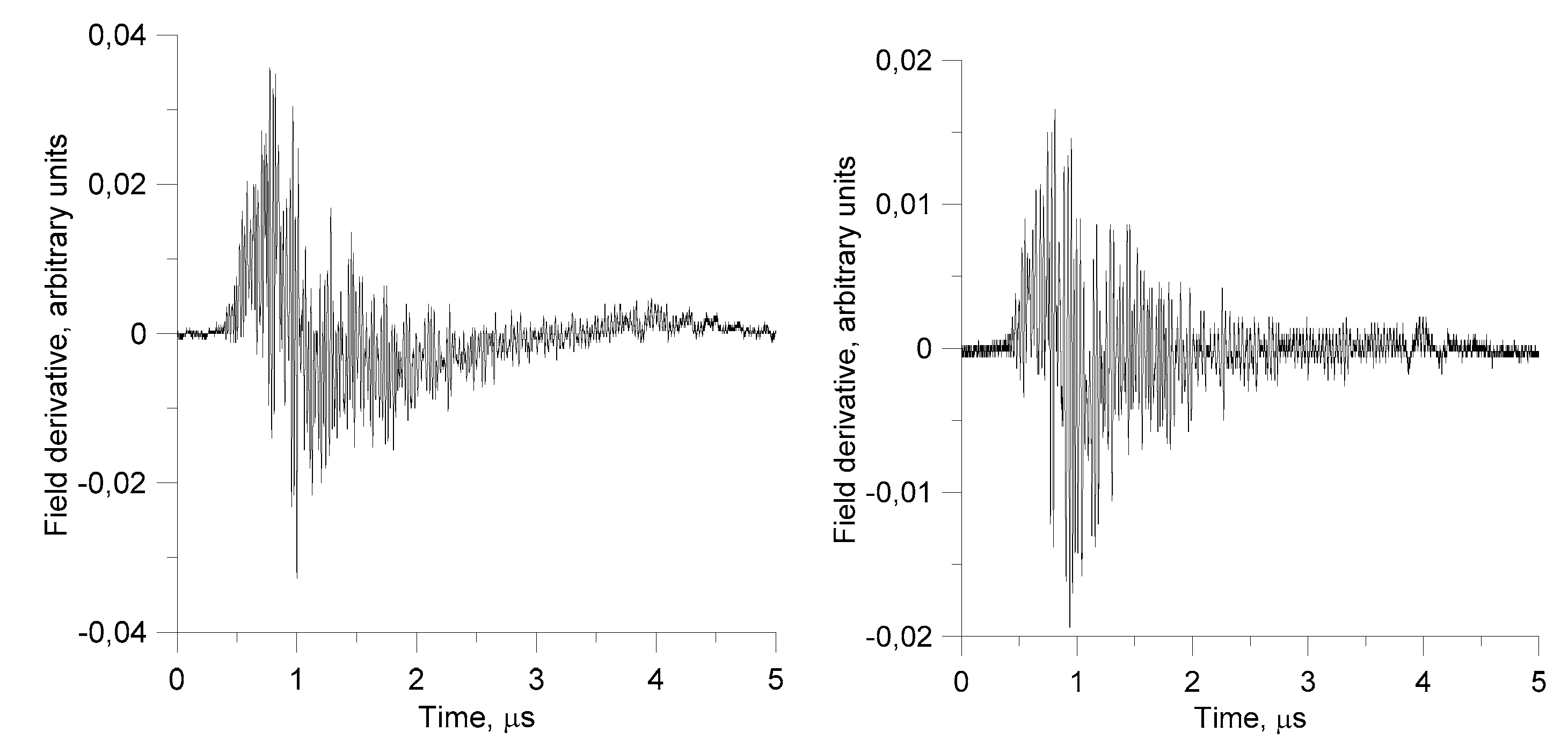
The typical duration of narrow bipolar pulses lies in the range of 10 to 20 μs. The polarity of the initial half cycle of these pulses can be either positive or negative. The zero crossing time of NBPs lies in the range of 3–10 μs [6,11]. Their initial peaks, when normalized to a common distance, are either comparable to or larger than those of return strokes. They appear to be rather smooth in field records, but high-resolution records show fine structure superimposed on these waveforms [12]. The presence of the fine structure is apparent when one observes the electric field time derivative of these pulses which shows a strong ragged structure which is not present in other high current events such as return strokes [2,14,15]. Figure 1 and Figure 2 show, respectively, examples of NBPs and their time derivatives measured in the study conducted by Karunarathne et al. [6] (and summarized by Bandara et al. [7]) and Gunasekara et al. [11] .
Narrow Bipolar Pulses are generated by bursts of electrical activity in the cloud which are referred to as Compact Intracloud Discharges (CID) or Narrow Bipolar Events in the current literature. These discharges usually occur in isolation without much electrical activity before or after the event, but sometimes they are observed prior to the initiation of lightning flashes. They are abundant in growing thunderstorms and mostly occur before the main electrical activity, i.e., the production of lightning flashes sets in. They usually take place at high altitudes, at heights around 10 km or more [3,4,16,17]. While CIDs are abundant in tropical thunderstorms [11], experimental observations show that CIDs are rare in Swedish thunderstorms [13].
Interferometric observations show that CIDs are involved with electrical activity that propagates over a rather short distance, several hundred meters or so, with speeds in the range of 3 × 10⁷ to 108 m/s with the upper theoretical bound being the speed of light [18].
Gurevich et al. [19] and Gurevich and Zybin [20] suggested the possibility that CIDs are generated by runaway avalanches. Marshall et al. [21] modeled the CID as a high current pulse propagating with speeds of 5 × 10⁷ m/s. Cooray et al. [14] modeled the CID as a series of runaway avalanches and explained the main features of the NBPs and the strong chaotic nature of the time derivatives of these fields. A study conducted by Babich et al. [22] made an attempt to simulate the CID as a relativistic avalanche. Nag and Rakov [5] inferred from the field waveshape of NBPs that they consist of some form of oscillating current ‘bouncing’ back and forth along the discharge channel. More recently, Rison et al. [23] and Tilles et al. [24] inferred from interferometric observations that CIDs are fast streamer discharges in virgin air which do not produce conducting channels.
Recently, several attempts were made to model CID’s as streamer bursts [25,26,27,28]. In [25,26], the CID is modeled as an interaction between two (or more) bipolar streamer structures formed in a strong large-scale electric field of a thundercloud and the features of the electromagnetic emission resulting from this interaction between streamer structures were examined. In the two publications [27,28], the idea of CIDs as a streamer burst was explored to study their physical parameters. In [27], the concept of propagating streamer systems inside the cloud environment as proposed by Griffith and Phelps [29] was utilized. Assuming that the streamer channel is of zero conductivity, the authors of [27] showed how the streamer system exhibits an initial exponential growth followed by a quadratic steady state. In [28], the radio spectrum of NBPs was investigated by modelling the CID as a burst of streamers. All the streamers in the burst were assumed to be initiated at the source location. Individual streamers were created at different times and these initiation times follow a certain probability distribution. The current moment of each streamer was assumed to follow a function whose time derivative matches the shape of the NBP. Using these ideas, the authors of [28] managed to obtain a radio spectrum of NBPs which agrees with experimental observations.
In the present paper, we will also model and simulate the CID as a streamer burst. However, our study differs in several aspects from the work described in [27,28]. In contrast to the work done by Attanasio et al. [27], we will attempt to connect the growth parameters of the streamer burst to the signature of the NBP and from that we will attempt to evaluate the temporal and spatial development of the streamer burst. Moreover, while providing a direct relationship between the streamer burst parameters and the radiation field of NBPs, we will also consider the effect of backward propagating currents along a weakly ionized streamer channel. Furthermore, while in [28] all the streamers in the burst were assumed to be originated at the source location, in our study, the growth of the streamer burst takes place as a result of streamer branching during the propagation of the burst. In other words, the streamer burst in our study may start with a small number of streamers and subsequently grow due to branching. We also provide an explanation for the emission of radiation during the propagation of streamers and we connect the growth of the streamer burst to the resulting NBP.
In what follows, we will first discuss the features of positive streamers as observed in the laboratory and then proceed to analyze the possible nature of the streamer bursts responsible for NBPs.
2. Characteristics of Positive Streamers
When the electric field in air increases beyond the threshold field necessary for cumulative ionization, i.e., the breakdown electric field, any free electron in air located in such an electric field can give rise to an electron avalanche. In electron avalanches, the number of electrons at the avalanche head increases exponentially with distance. At standard atmospheric pressure when the number of electrons at the avalanche head reaches about 108, the avalanche will be transformed into a streamer discharge [30]. The reason for this is the following. When the number of the electrons reaches this value, the distortion of the electric field by the space charge located at the head of the avalanche becomes so large that the positive space charge at the avalanche head starts attracting more avalanches towards it and with the aid of these avalanches the streamer propagates in a background electric field that is lower than the breakdown electric field.
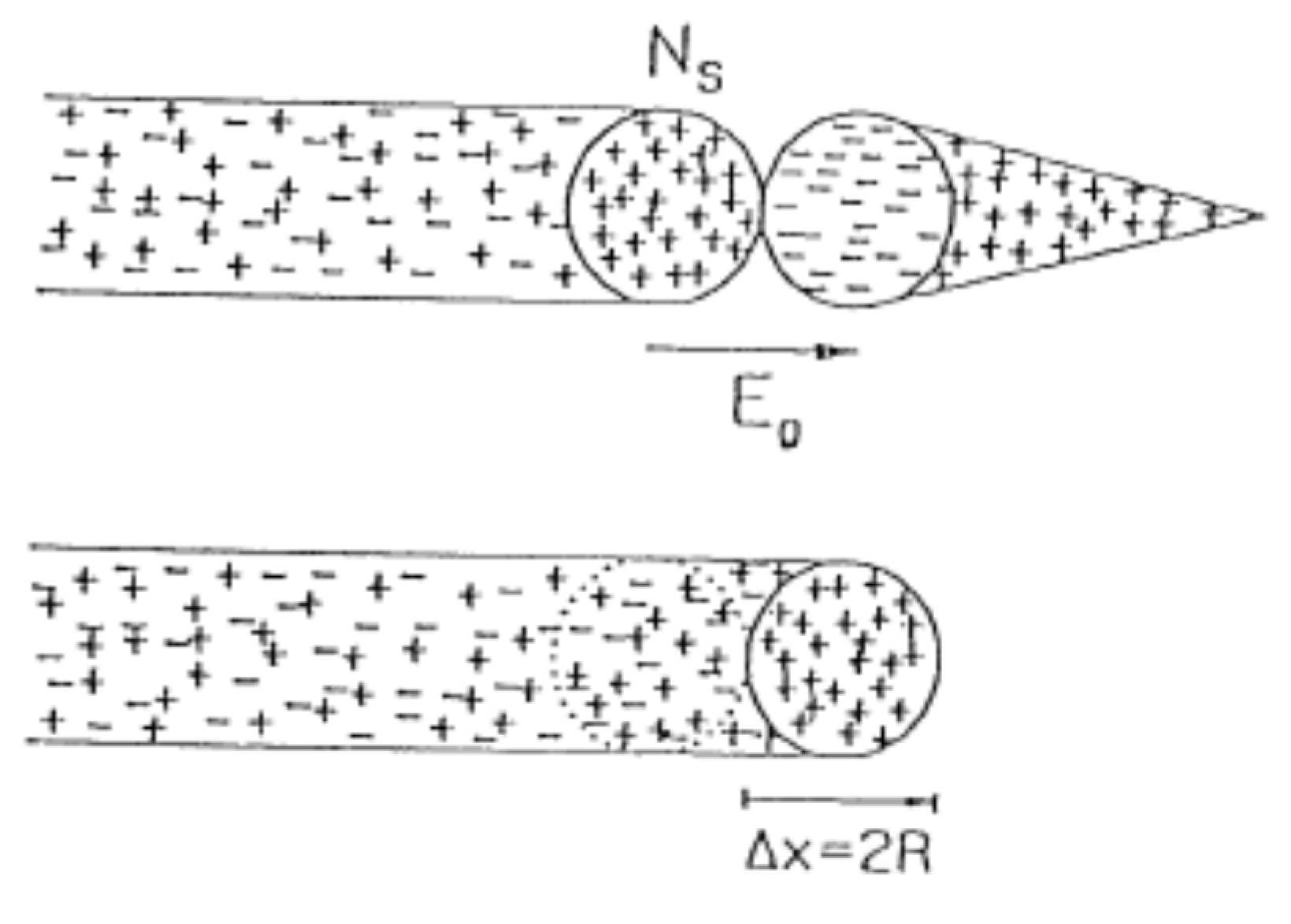
A schematic representation of the propagation of a positive streamer is shown in Figure 3. The high electric field produced by the positive charge at the streamer head attracts secondary avalanches towards it. These avalanches neutralize the positive space charge of the original streamer head leaving behind an equal amount of positive space charge at a location slightly ahead of the previous head. In this way, the streamer propagates ahead. Thus, the streamer can be visualized in the ideal case as a propagation of a localized positive space charge in the background electric field.
In the laboratory under standard atmospheric pressure, positive streamers were observed to travel at speeds in the range 2 × 10⁵ to 5 × 10⁶ m/s [31,32]. The background electric field necessary for their propagation at standard atmospheric pressure is estimated to be about 5 × 10⁵ V/m [30,33]. The diameter of the streamer channel at atmospheric pressure may lie in the range of hundreds of μm to several mm [31,32]. The streamer diameter is observed to increase with increasing applied voltage or with increasing background electric field. The maximum value of the streamer diameter observed in experiments is about 3 mm [31,32].
Experiments and theory indicate that the background electric field necessary for streamer propagation, the streamer diameter, and the charge at the streamer head depend on the atmospheric pressure in which the streamer is propagating [34,35]. The background electric field necessary for positive streamer propagation decreases with decreasing pressure and at a pressure corresponding to 0.5 bar it may decrease to about 1.5 × 10⁵ to 2.0 × 10⁵ V/m and at 0.3 bar it may decrease to about 1.0 × 10⁵ V/m [34]. At altitudes between about 10 and 12 km, where the CID takes place, the atmospheric pressure is about 0.25 and 0.19 bar, respectively, and, thus the background electric field necessary for stable streamer propagation may decrease further. The similarity laws indicate that the diameter of the streamer increases as , where is the standard atmospheric pressure, do is the corresponding streamer diameter, and is the diameter at air pressure equal to [35]. The experimental data also indicate that the streamer diameter increases almost linearly with atmospheric pressure [31,32]. The charge at the streamer head also increases according to the relation , where is the charge at the streamer head under standard atmospheric pressure and is the streamer head charge at atmospheric pressure [35]. The similarity laws indicate that the electron drift velocity does not change with pressure [35]. The laboratory experiments show that the streamer speed increases almost with the square of the diameter of the streamer head [31,32]. The reason for this is the increase in the active region of the streamer channel with increasing diameter. Since the active region of the streamer increases with decreasing pressure, it is possible that the streamer speeds also increase with decreasing pressure.
3. CID as a Streamer Burst and the Current Associated with the Streamers
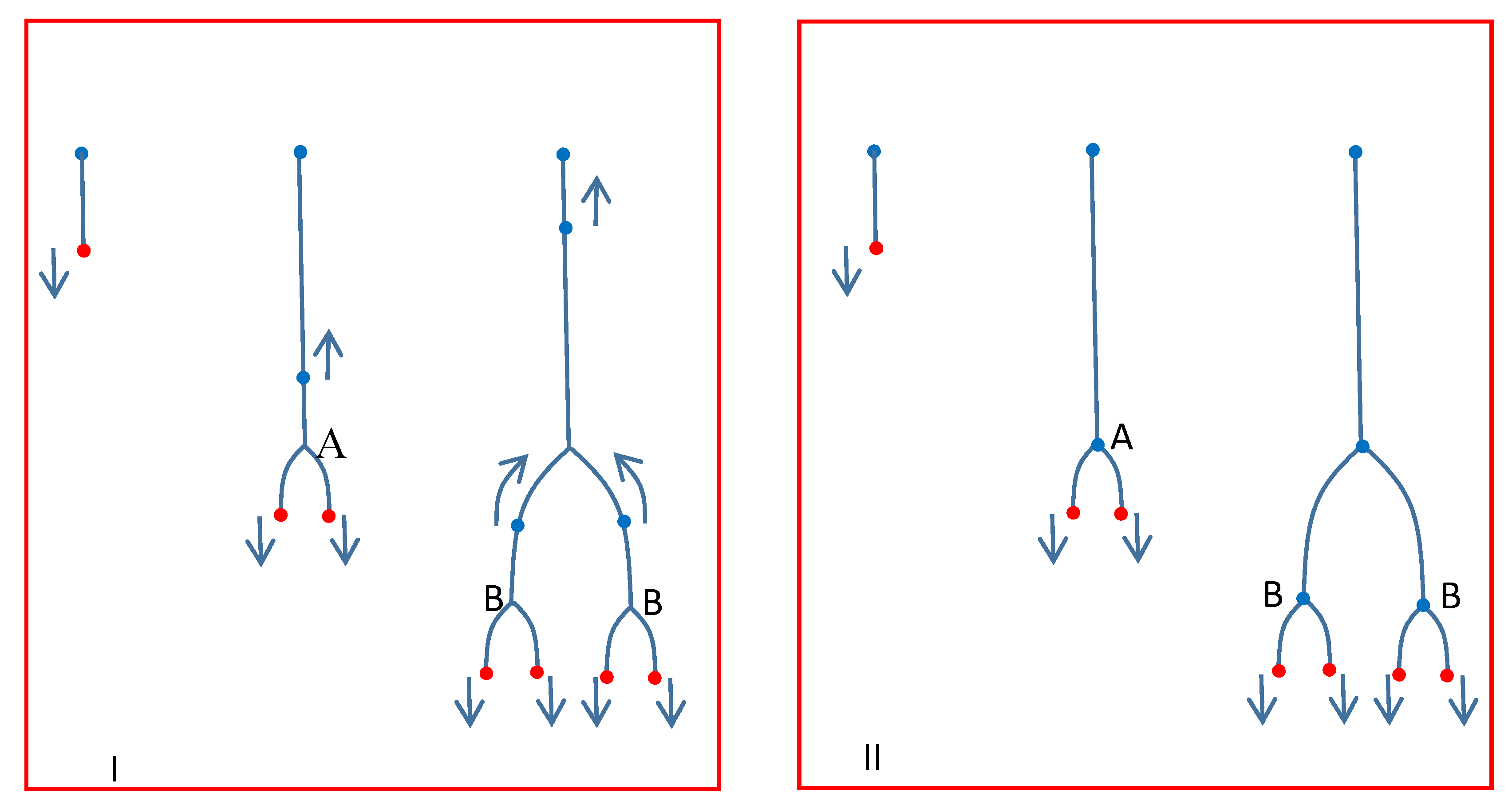
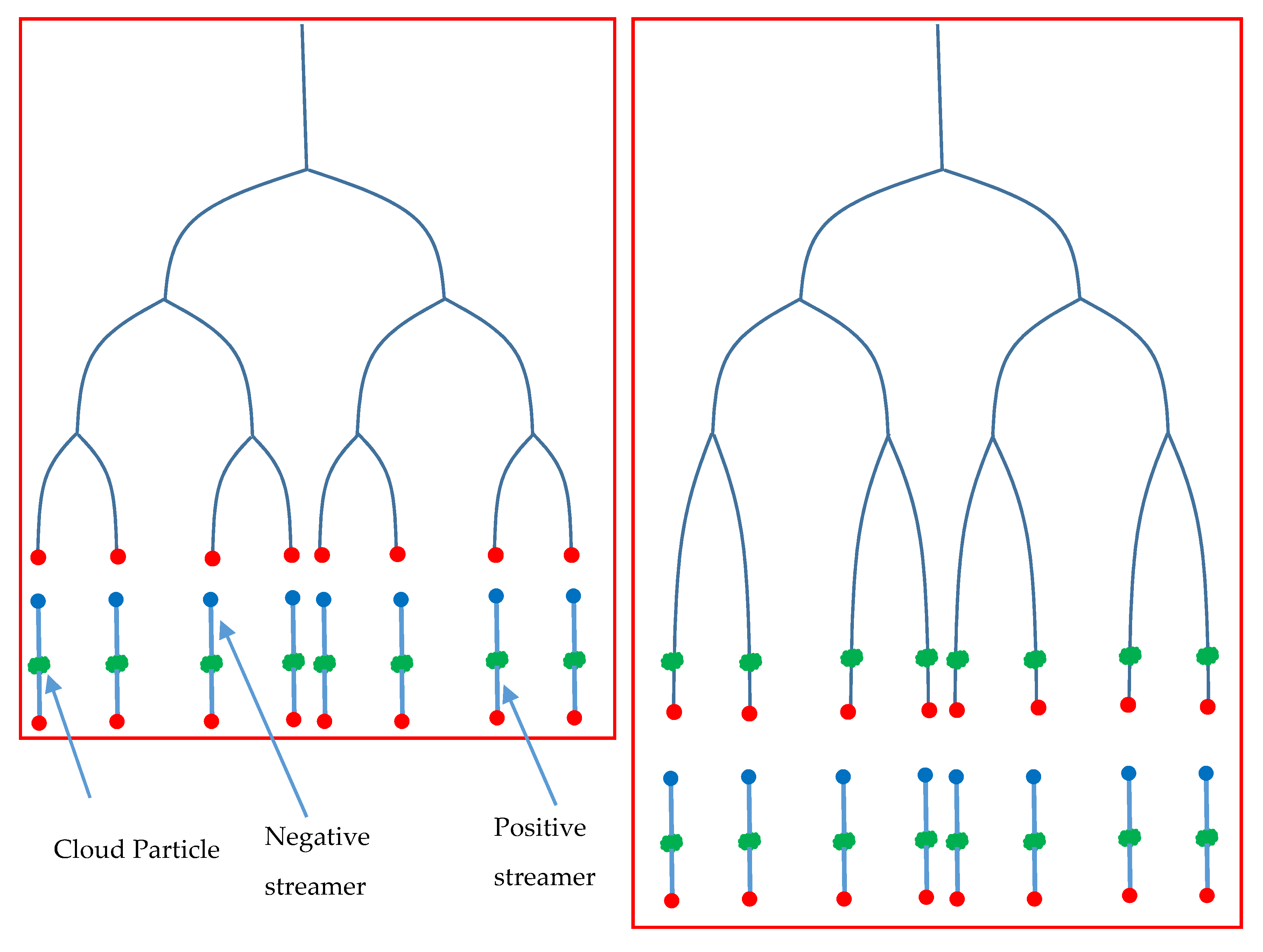
In the analysis to follow, we will utilize the ideal picture of a streamer channel presented above and treat the propagation of a streamer channel as a propagation of a spherical charge distribution. Furthermore, according to this picture, since the electrons in the secondary avalanches will be neutralized by the positive charge, a backward propagating electron distribution or current is generated only at the instant of the creation of the streamer head. Once a streamer starts propagating, a backward propagating electron distribution is created only when the streamer is branched. This is the case because, during branching of the streamer, a new positive streamer head is generated and the additional electrons created during the process will propagate towards the origin of the streamer. The backward moving current pulse is assumed to be identical to the forward moving current pulse associated with the positive streamer head except for the polarity. The effect of dispersion of the backward moving current will also be considered later. This scenario is depicted in Figure 4 (Box I). In this diagram, the spherical charge distribution associated with the streamer head is depicted by red dots. The negative charge distribution associated with the electrons is depicted by blue dots. This is the scenario that we will be using in estimating the electromagnetic fields generated by the streamer burst. However, if the conductivity of the streamer channel is zero, the negative charge remains at the same location where it was created (the assumption made in [27]). We will consider this case too in our analysis (Figure 4, Box II).
Let us assume that CID is a streamer burst. We assume that it is not associated with or it will not give rise to a hot conducting channel [23]. A possible justification for this assumption will be given later. Assume that the streamer burst is initiated by a certain number of streamers. Following the description of the movement of positive streamers given earlier, the movement of a streamer head is represented by a movement of a spherical charge pocket. This in turn can be represented by a propagating current pulse. If the speed of propagation of the streamers is , which we assume to be uniform, and the radius of the spherical charge distribution at the streamer head (note that this is the same as the radius of the streamer channel) is , the duration of the current pulse associated with the propagating streamer head, , will be equal to . Let us assume that the overall charge distribution in the spherical charge pocket is Gaussian. Then, the current waveform associated with the movement of the streamer head can be represented by
In the above equation, is the total charge of the spherical charge pocket at the streamer head and . In the simulation, the charge on the streamer head is assumed to be C, which corresponds to elementary charges. At standard atmospheric pressure, the streamer head charge is about electrons and, at low pressures corresponding to an altitude of 10 km, a value of is reasonable according to similarity laws. In order to shift the Gaussian function to the positive times, we have used in the exponent with the understanding that the current pulse will go to almost zero for times less than or equal to zero. This is the expression for the streamer current that we have used in our analysis. However, observe that, for speeds of propagation of CIDs in the range of m/s or more, the duration of the current pulse is in the sub-nanosecond domain even for low pressure expanded streamer radii in the cm range [31,32]. For example, if equal to 0.01 m, = 0.33 ns. Thus, for calculations pertinent to time resolutions larger than about 1 ns, the current pulse associated with the streamer head can be represented by a Dirac delta function. That is,
In the above equation, is the charge on the streamer head.
According to the scenario we use in this simulation, at a branch point, a forward moving streamer head of charge will be converted to two forward moving streamer heads each carrying a charge equal to . This is depicted in Figure 4. Since the branching process leads to a creation of a new streamer head with charge , in order to maintain charge conservation, an equal amount of negative charge is also created at the same location. There are three physical scenarios that are of interest to be investigated concerning the fate of this negative charge. The first case is that this charge remains where it is located while the positive charge associated with the streamer head moves forward. The second case is that this charge maintains the same concentration but moves backward towards the origin of the streamer burst with speeds less than or equal to . The third case corresponds to the situation of strong dispersion of the backward current taking place during its propagation, making the duration of the pulse much longer. In the two latter cases, the backward moving electron current is also given by an expression similar to that given by Equation (1). That is,
If the backward current does not disperse as it travels along the weakly conducting channel, and . If the backward current disperses, and .
Equations (1)–(3) describe the current elements of the streamer burst. The next step is to write down expressions for the radiation generated during the initiation and branching of the streamer channel.
4. Radiation Field Generated by the Initiation and Branching of a Streamer Channel
The streamer system radiates every time a streamer is initiated or when a new streamer head is created during the branching of a streamer. This is the case because it is only during the initiation of a new streamer head that new charges are accelerated from rest to move (note that in the case of positive charge it is an effective movement) with the speed of the streamer. In the calculations to follow, we assume that during streamer branching both branches will propagate almost in a vertical direction. Without this assumption, one has to take into account the branching angle in calculating the radiation field.
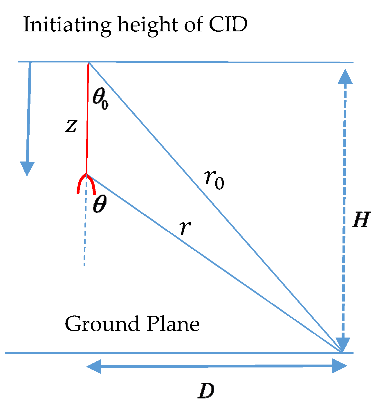
Consider the initiation of a single streamer from the origin of the streamer burst (i.e., at ) at time t = 0. We assume that the streamer moves vertically downwards with uniform speed denoted by . We assume that the ground is perfectly conducting and its effects on the radiation field are taken into account by an ‘image streamer’ in the ground. The relevant geometry is shown in Figure 5. First, the initiation of the streamer at will give rise to a vertical radiation field at ground level, and this radiation field can be described by the equation [36,37,38]
In Equation (4), Subscript 1 refers to the radiation generated at the initiation of the streamer. Note that we use the sign convention where the electric field directed out of the ground is considered positive.
Assume that the streamer will make a branch when its head is located at a distance from its origin (see Figure 5). If the negative charge that is being created is also assumed to propagate backwards, the radiation field produced during the branching consists of three pulses. The first radiation pulse is created by the forward movement of the positive charge head of the new branch. The second radiation pulse is created by the backward movement of negative charge associated with the newly created streamer head and the third radiation pulse is created by the termination of the backward moving negative current pulse at the origin of the streamer burst. The radiation fields generated at the initiation of these current pulses can be described mathematically as follows [36,37]:
The parameters of the above equations are also defined in Figure 5. Similarly, the radiation field produced during the termination of the backward moving current pulse at the origin of the streamer burst (i.e., ) is given by
In the above equations, subscript 2 in Equation (5) refers to the radiation generated by the forward moving positive charge, subscript 3 in Equation (6) refers to the radiation generated by the backward moving negative charge, and subscript 4 in Equation (7) refers to the radiation generated when the backward moving negative charge is stopped at the streamer origin.
The above equations describe completely the radiation fields produced during a single branching event. If the negative charge created during the branching event remains where it was created, then the total radiation field generated by the branching process can be described by Equation (5) alone. The distant radiation field of the CID or the NBP is created by the cumulative effect of the radiation fields generated by the branching of the forward moving streamers. Now, we are ready to write down an expression for the electric field generated by the streamer burst.
5. Electric Field Generated by the Streamer Burst
First of all, from the analysis presented in the previous section, one can note that the temporal variation of the radiation field of the streamer burst is controlled by the time evolution of the number of streamer heads of the streamer burst as a function of time. In the growing stage of the streamer burst, the number of streamer heads will increase as a function of time due to branching and, in the decaying stage, the total number of propagating streamer heads starts to decrease (due to the termination of some of the streamer channels) and eventually reaches zero. Thus, the total number of propagating streamer heads can be mathematically represented by a function that increases initially with time, reaches a peak, and then decays. As we will show later, this function can be inferred directly from the measured radiation field of the CID. For the moment, let us denote the growth and decay of the streamer heads in the streamer burst as a function of time by . The parameter is the number of streamer heads moving forward at any given time t. The way in which the number of streamer heads vary with z, i.e., , can be obtained by replacing t by z/vs. Note that n can be expressed equivalently as a function of z (location of streamer head) or t (time taken by the streamer to reach z). Once this function is defined, we will be in a position to write down the expressions for the electric fields produced by the CID.
The electric field generated by the streamer burst can be divided into radiation field, velocity field and static field [36,37]. The radiation field is produced by accelerating charges, for example when currents are initiated or terminated. The velocity field is the modified Coulomb field generated by the moving charges associated with the current, and the static field is the Coulomb field produced by the stationary charges. In the streamer system under consideration, as we have seen in Section 4, radiation fields are produced by the currents associated with the positive charge of the newly created streamer heads, the currents associated with the negative charge of the newly created streamer heads moving towards the origin of the streamer burst, and the radiation generated as these backward moving currents are terminated at the origin of the streamer burst. Velocity fields are generated by current pulses moving forward (positive charge) and backwards (negative charge) inside the streamer burst and the static fields are produced by charges deposited by the terminated positive heads (positive charge) and the charges deposited at the origin by the backward moving currents (negative charge). Let us now write down expressions for these field components.
5.1. Radiation Field
Let us assign for the time at which the streamer burst is initiated at height above the perfectly conducting ground plane. The relevant geometry is shown in Figure 6. The burst moves towards ground with uniform speed . As before, we assign to the origin of the streamer burst and the z coordinate increases towards the ground. Let us consider the radiation emitted by the events taking place in the streamer burst when it travels from to . The number of new streamer heads generated as the streamer burst travels across this elementary distance is
The positive current caused by the newly created streamer heads, say , when the streamer burst travels from to is given by
Thus, the radiation field generated by the newly created positive current pulses moving towards ground is
In the above equation, is the location at which the cessation of the streamer burst takes place. Similarly, the radiation field generated by the current associated with the negative charge moving towards the streamer origin is given by
Furthermore, the radiation field generated by the termination of this current at the streamer origin is
In Equations (11) and (12), is the distance from the origin at which becomes negative. In writing down Equations (11) and (12) we are assuming that no new streamer heads are created in the region where is negative. The total radiation field generated by the streamer burst can be obtained by summing up the different contributions. That is,
Once the speed and the time evolution of the streamer heads are specified, one can calculate the resulting radiation field from the equations given above. If the negative charge is assumed to be localized at the place of creation, the radiation field is given by Equation (10) alone. Note also that we have assumed that all the streamers are vertically oriented.
5.2. Velocity Field Generated by the Streamer Burst
The velocity field is created both by the forward and backward moving current pulses located inside the elementary spatial distance . The number of current pulses (or streamer heads) moving forward and located within the spatial distance is equal to . Thus, the velocity field generated by the forward moving current is [36,37]:
The total velocity field generated by the forward moving current is
Before writing down the expression for the velocity field caused by the backward moving currents, it is necessary to express the backward moving current flowing through as a function of time. The geometry necessary for the calculation is given in Figure 7. First, observe that the backward moving currents associated with all the new heads created in the region ahead of the location z will flow through the elementary length dz. Consider an elementary length located at where . The current at generated by the new heads created at is given by
Thus, the total backward current moving across the element is given by
From this, the velocity field generated by the backward moving electron current is
The total velocity field is given by the sum of and .
5.3. Static Field Generated by the Streamer Burst
During the movement of the streamer burst, there are two sources that will generate a static field. The first source is the negative charge that will accumulate due to the termination of backward moving negative current at the origin of the streamer burst. If we assume that the negative charge does not travel backwards, one has to modify the static field appropriately as we will show later. The other source is the positive charge that will accumulate at the forward end of the streamer burst due to the cessation of the propagation of the streamer heads. Now, the backward current reaching the origin of the streamer burst as a function of time is given by
From this, one can estimate the magnitude of the negative charge that will accumulate at as
Thus, the electrostatic field produced by the accumulation of negative charge at the origin of the streamer burst is (note that the field is directed out of the ground)
Now, let us consider the accumulation of positive charge along the path of the streamer burst. First, observe that the accumulation of positive charge takes place in the region where is negative, that is, in the region where the termination of the streamer heads is taking place. Consider an element at distance from the origin. The value of is such that is negative. The positive charge deposited in element is
The electric field produced at ground level by this positive charge is given by
Substituting for from Equation (22), the total static field produced by the positive charge accumulated along the streamer burst can be written as
In the above equation, is the distance from the origin of the streamer burst when becomes negative. Thus, the total static field produced by the streamer burst is given by
If we assume that the negative charge remains localized at the place of creation, then the electric field generated by the negative charge is
The total field in this case is given by
6. Growth Parameters of Streamer Burst That Best Represent CID
Equations (8)–(27) represent the components of the electric field produced by the streamer burst. The next task is to estimate the growth parameters, i.e., (or ), pertinent to the NBP. In principle, this can be estimated directly by the field signature of the NBP. If the time resolution needed in the calculations is such that and , then, for all practical purposes, the forward and backward moving current can be represented by a Dirac delta function and the growth curve of the streamer burst can be obtained analytically from the field signature of NBPs. If and , the growth curve can be obtained through numerical means from the NBP. Let us consider the case that and . First, consider the case of a non-conducting streamer channel. In this case, the radiation field generated by the streamer burst can be described by the equation
If the distance is much larger than the length of the streamer burst, the above equation reduces to
From this, one obtains
Thus, if the speed and the distance to the location of the NBP is known, the growth curve can be obtained directly from Equation (30). This shows that the growth curve of the streamer burst is directly proportional to the integral of the NBP.
If one considers the backward moving current (i.e., partially conducting streamer channel), the radiation field is given by
Following a similar analysis, we obtain
Note that in the last term the time derivative is evaluated at time t/2. This can be simplified to
This equation can be easily solved numerically using an iterative method to obtain the growth curve. Note that if 2zm < zmax then for times greater than 2zm/vs the radiation field is given by Equation (29). In the case and , the growth curve can be extracted numerically from Equations (28) and (31).
In order to obtain a function that can be mathematically manipulated easily, we have extracted the growth curve from a large number of NBPs obtained in Sri Lanka from the study conducted by Gunasekara et al. [11]. We observed that the overall features of the growth curve as a function of time can be described by the function given below with the values of and in the range, respectively, of 0.1–0.4 μs and 2–10 μs best representing the measured NBPs:
The particular form of the function given in Equation (34) was selected to make sure that the second derivative of this function, which is related to the time derivative of the radiation field, behaves in a physically acceptable manner. In this expression, the value of decides the amplitude of the NBP at a given distance. The growth curve as a function of , i.e., n(z) can be obtained from Equation (34) by replacing by . If the time of initiation of the streamer burst is assigned to = 0, the number of new streamer heads created during the time interval is given by . The calculated NBPs using this growth curve with = 0.1 μs and = 4 μs are depicted in Figure 8. In the calculation, we have selected the value of to make the peak of the radiation field at 100 km equal to 10 V/m and the charge on the streamer head is assumed to be C, which corresponds, as mentioned earlier, to elementary charges. Note also that the value of we need to match a given amplitude of the radiation field depends on the value of selected in the calculation. Furthermore, the speed of the streamer burst is kept constant at 3 × 10⁷ m/s in the calculation. In the study conducted by Gunasekara et al. [11], the risetime, zero crossing time, and the duration of the NBPs were about 0.6–1 μs, 3–4 μs, and 16–20 μs, respectively. The parameters of the calculated NBPs agree reasonably well with these parameters. Of course, observe that the growth curve can be extracted directly from the measured NBPs.
7. Characteristics of the Streamer Bursts Giving Rise to NBPs
7.1. The Growth Rate of Streamer Heads and the Current
Figure 9 shows the total number of streamer heads propagating and the number of new streamer heads created as a function of z corresponding to the radiation fields depicted in Figure 8.
Observe from these diagrams that the number of streamer heads propagating forward at a given distance from the origin (Figure 9a) increases initially, reaches a peak, and then decreases. Furthermore, in Figure 9b, the number of newly created streamer heads increases initially and it then goes on to decrease and becomes negative with increasing distance. The meaning of the negative number, as mentioned earlier, is that, instead of creation, more streamer heads are being stopped on the way.
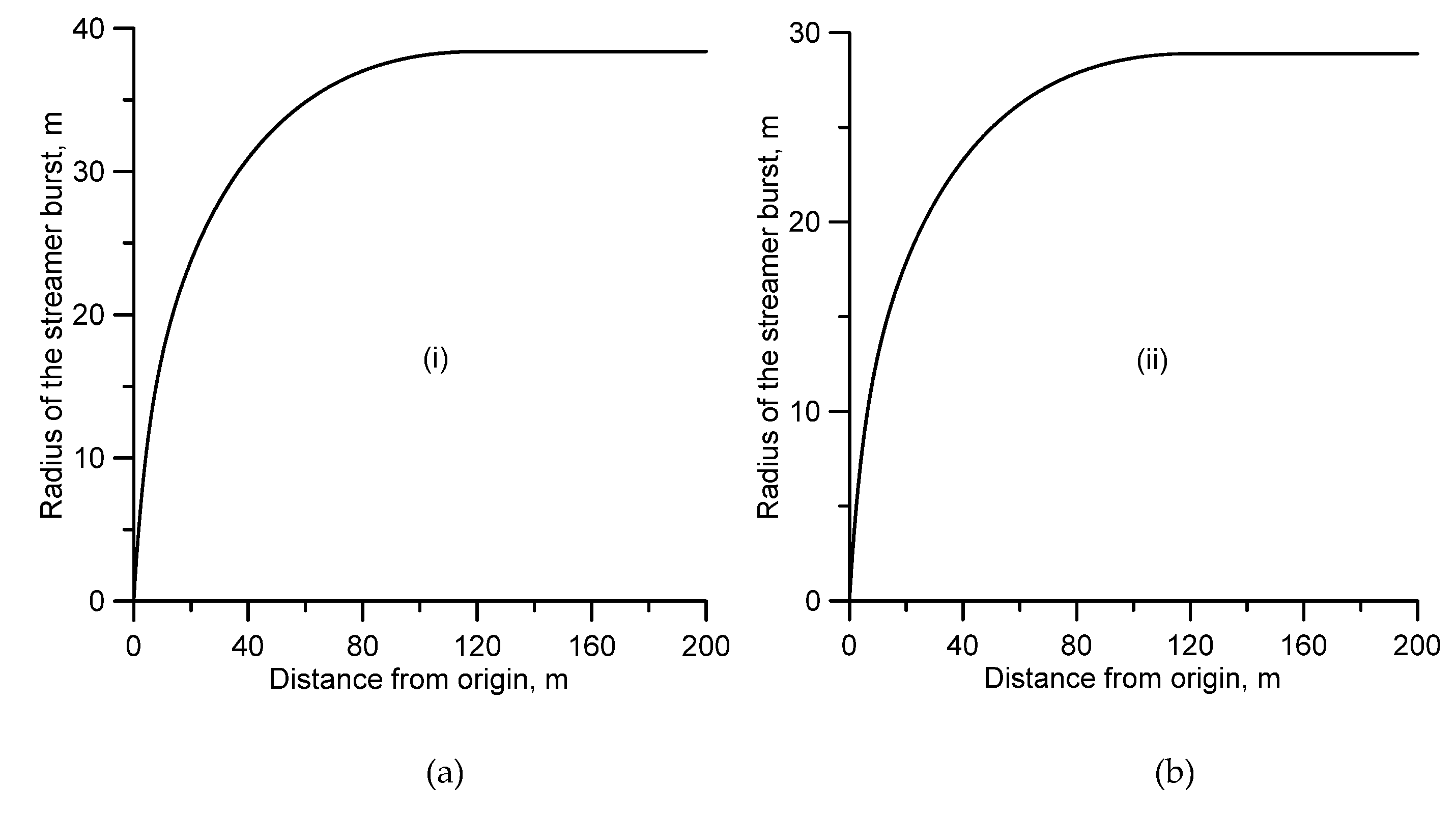
Note that, due to the short duration of the current pulse associated with the charge distribution of the streamer head, the current associated with the CID is compressed almost to a very thin region in the longitudinal direction. Thus, the CID appears as a forward moving very thin current sheet whose amplitude is modulated as it propagates downwards. Behind this front, negative charges propagate towards the origin of the CID. The current associated with the forward moving front of the streamer burst is shown in Figure 9c. Note that this current is equal to the sum of the currents associated with the forward moving streamer heads. This is the case because it is obtained by multiplying the number of streamer heads in curve (i) of Figure 9a by the current associated with a single streamer. If all the forward moving streamer heads are located on a single horizontal plane then the peak current associated with the front can reach a peak value of about 4.5 × 10⁸ A. However, in reality there will be a vertical spread in the location of the forward moving streamer heads and this will lead to a reduction in the current associated with the front will be reduced considerably. For example, if all the forward moving streamer heads are located on a single horizontal plane the width of the streamer front will be about 1 cm and the duration of the current associated with the streamer front will be about 0.5 ns. If the forward moving streamer heads are dispersed along a vertical direction so that the width of the streamer front is about a meter, the peak current will be reduced by a factor of hundred. Observe that the current density associated with this current sheet needs not be very high because the streamer front can have a cross section of hundreds of square meters. A rough value of the radial expansion of the streamer burst can be calculated as follows. First observe that the minimum radial distance between two streamer heads cannot be smaller than the active region of each streamer head. If the distance is smaller, they will start competing for the same electron avalanches and the consequence would be that one will grow at the expense of the other. Let us denote the lateral extension (or radius) of this active region by . Thus, at a minimum, each streamer head takes an area of about in a horizontal plane so that it will not interact with other streamers. The area of the cross section of the streamer burst at a given value of is equal to . As starts decreasing, the area remains at the value corresponding to . This is the case because, as the demise of the streamer heads takes place, the remaining streamers will continue along the same direction that they were traveling at the location where the peak of was reached.
At standard atmospheric pressure, the active region of a streamer head is about 100 μm and, in the low-pressure atmosphere, where CIDs usually take place, it may increase to about 1 mm following similarity laws [30,35]. Using this value as a measure of the minimum separation between the streamer heads and assuming that the cross section of the streamer burst is approximately spherical, the calculated lateral expansion (or the radius) of the streamer burst as a function of is shown in Figure 10 for the two cases considered earlier. Note that the expansion of the streamer burst is nearly exponential initially, but, as time goes on, the expansion stops and the radius of the streamer burst becomes constant. Note that, in reality, the separation between the streamer heads could be larger than the active region of the streamer heads (and also the radius of the active region could be larger than 1mm) and for this reason the calculated value has to be taken as a lower bound.
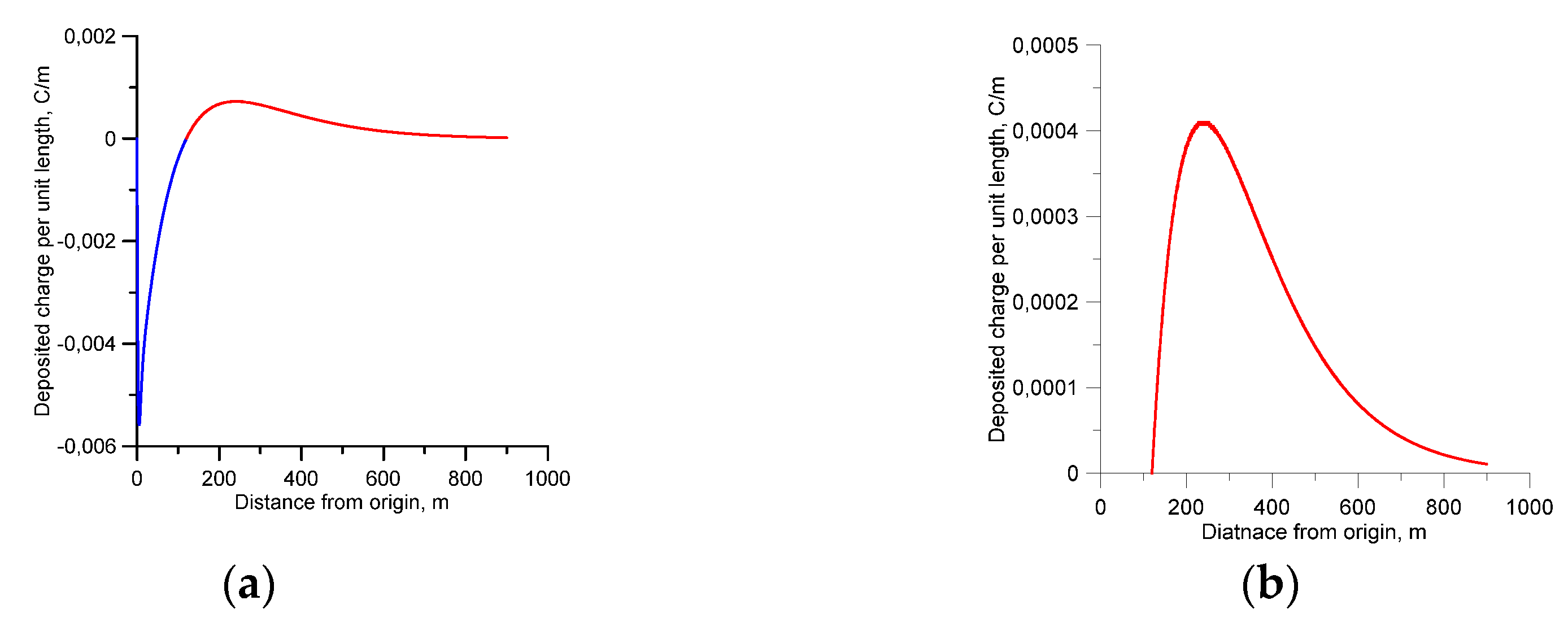
7.2. Charge Deposition in Space by the Streamer Burst
The positive charge deposited by the streamer burst as a function of the z-coordinate is shown in Figure 11 for the two cases considered earlier. Figure 11a shows the charge distribution for a non-conducting streamer channel, i.e., negative charge remains where it is created. In this case, negative charge is deposited close to the streamer origin and the positive charge is deposited away from it. Figure 11b shows the charge distribution for a partially conducting streamer channel where the negative charge is transported to the streamer origin. In this case, only positive charge will be deposited along the streamer tracks. The positive charge deposited and the charge moment associated with these two cases are 0.24 C, 74 Cm, and 0.13 C, 46 Cm, respectively. For a given peak value of NBP, the amount of charge deposited and the current moment increases as the width of the NBP increases, i.e., with increasing . For values of around 10 μs, a CID associated with a 10 V/m NBP at 100 km, the charge deposited, and the charge moment reach about 0.5 C and 326 Cm, and 0.45 C and 256 Cm, respectively, for the non-conducting and conducting streamer channels. For a given width of the NBP, these parameters increase linearly with the peak value of the NBP. Recall that in our case the peak value of NBPs at 100 km is 10 V/m. Note also that, for a given set of growth parameters, the charge moment increases with increasing speed. This is the case because charges are displaced over longer lengths as the speed increases.
7.3. The Effect of Dispersion of the Backward Moving Current
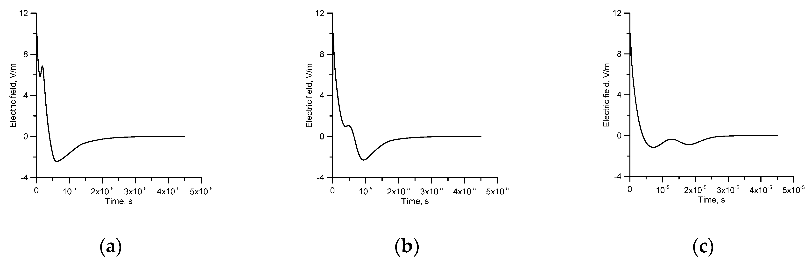
In the analysis presented earlier, we have assumed that the negative charges will propagate backwards keeping the same concentration as the head of the streamer, i.e., . However, the streamer channel is only weakly conducting and strong dispersion of current waves propagating along this channel will take place. Thus, the assumption that the negative charge will propagate without dispersion is not physically reasonable. In order to correct for this, we have to assume the time constant of the backward current to be much longer than the value of about 0.5 ns estimated for forward moving current pulses. The effect of increasing the duration (i.e., ) of the backward moving electron current is shown in Figure 12. Observe how the waveforms will be modified by the dispersion of the backward moving current waveform. Depending on the amount of dispersion, which may vary from one burst to another, it can give rise to either subsidiary peaks or provide oscillation in the tail of the NBPs. As depicted in Figure 1, both of these features have been detected in the experimentally observed NBPs. Interestingly, the oscillations in the tail of NBPs were explained as bouncing current waveforms along a conducting channel by Nag and Rakov [5]. Here, we provide an alternative explanation for this feature.
7.4. Reasons for the Finer Features of the NBPs
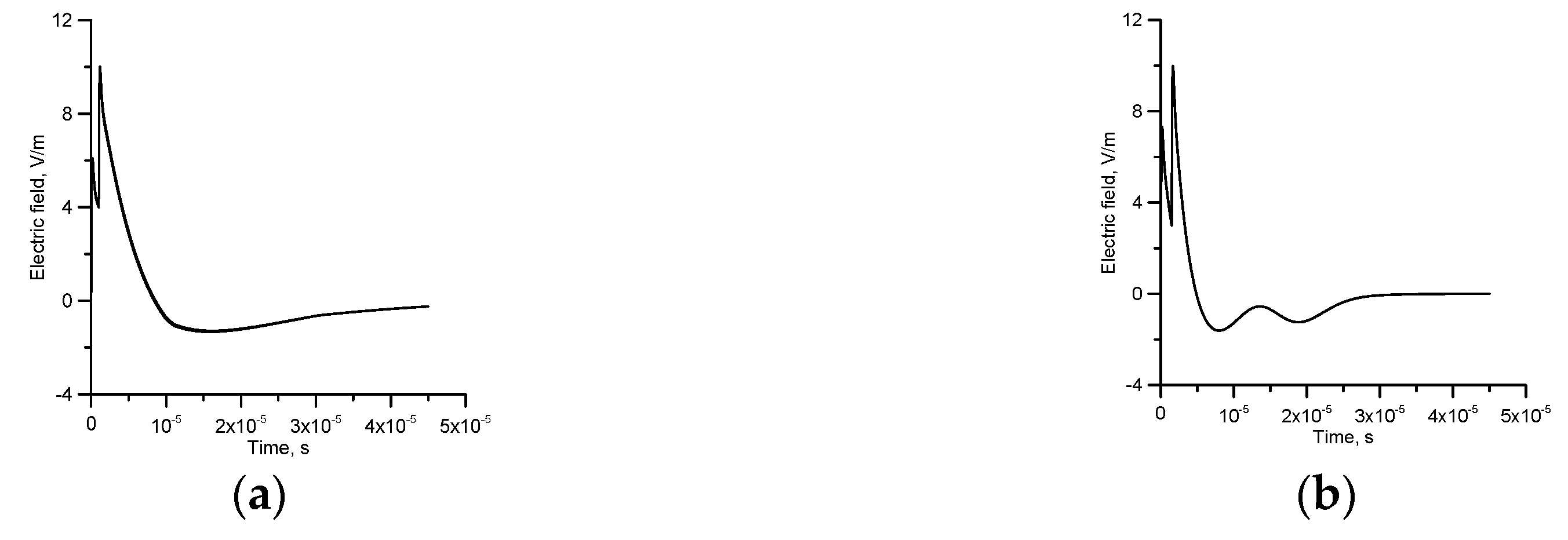
The information gathered on NBPs recently shows that some of the narrow bipolar pulses are characterized by fine structure such as several peaks in the rising part as illustrated by the results obtained by Karunaratne et al. [6] and Leal et al. [8]. As shown in Section 7.3, some of this fine structure could very well be due to the dispersion of the backward moving electron current. In the case of laboratory experiments, if a voltage large enough to initiate streamers is applied to an electrode, one may encounter multiple streamer bursts from the electrode [31,32,33]. The first burst may reduce the electric field in the vicinity of the electrode, but, as the space charge drifts off, another streamer burst could be initiated. The same physical phenomenon may also happen in the case of the streamer bursts in the cloud: once initiated, instead of one streamer burst, several streamer bursts could be generated from the same region. Moreover, initiation of multiple streamer bursts could be enhanced by the negative charge reaching the streamer origin at later times. Thus, the CID may contain several streamer bursts that may occur in succession from the same region of origin of the burst. The effect of multiple streamer bursts on the radiation fields is shown in Figure 13. In this calculation, we have assumed that individual streamer bursts are identical in their temporal behavior but they are displaced in time. We have simulated only two streamer bursts. Note that fine structure similar to that observed in experiments (see Figure 1) could very well be produced by two or more streamer bursts originating from the same place.
7.5. The Effect of the Random Nature of the Branching Process
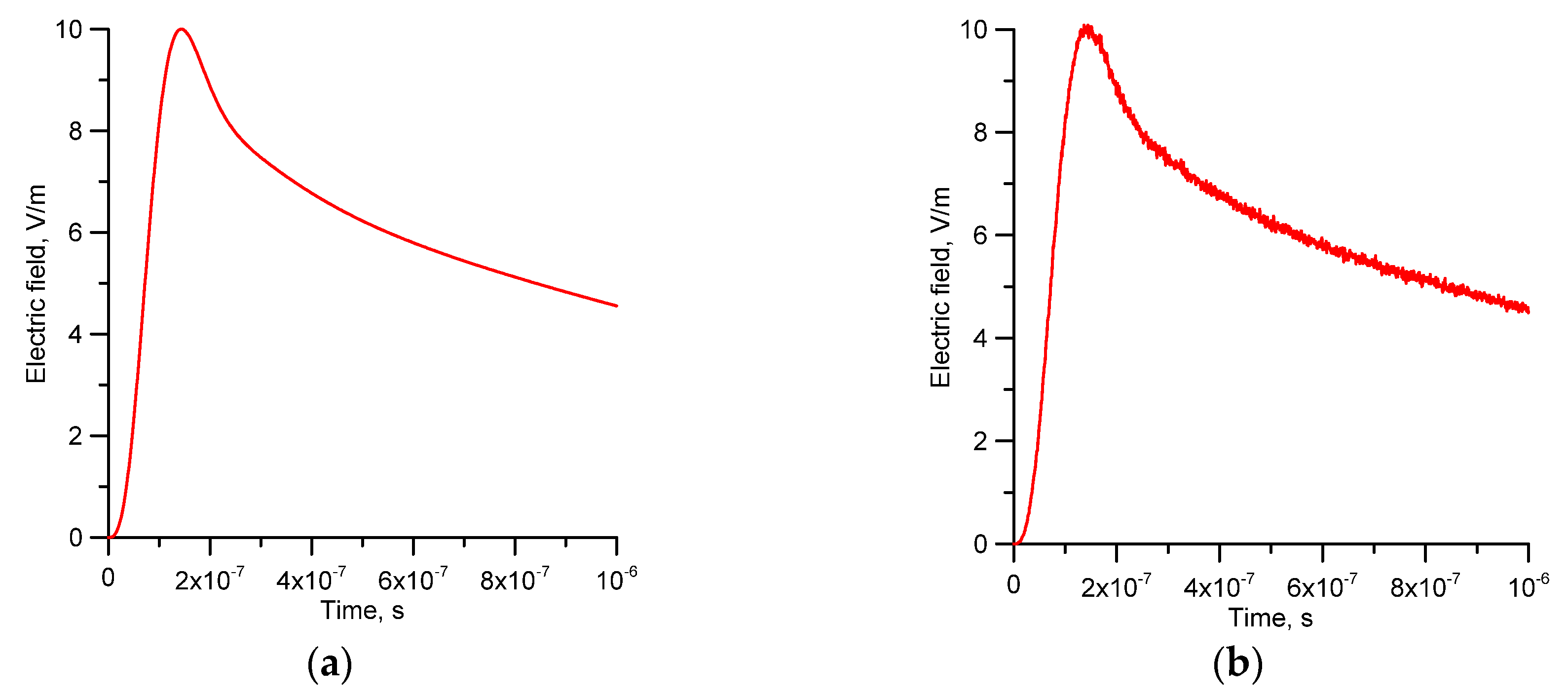
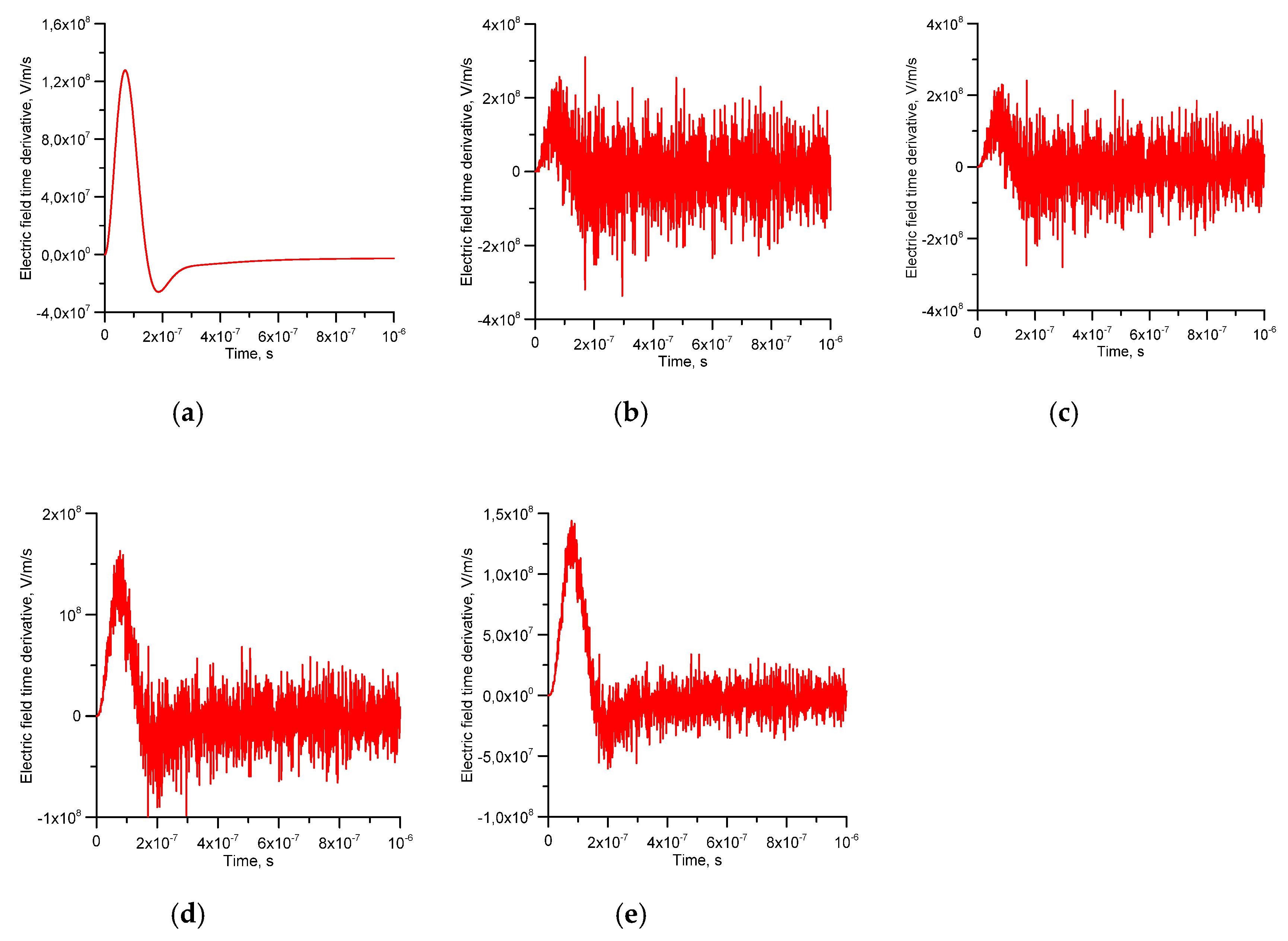
First, observe that the radiation amplitude of the NBP at a small time interval is decided by the number of new heads created during that time interval. The new heads are created through the branching process. If we could resolve the experimentally observed growth curve in nanosecond resolution, the number of streamer heads created over a given time interval may not follow a smooth curve, as shown in Figure 9a. This is the case because all the streamers do not branch at the same time, and there is some ‘randomness’ involved in the generation of new streamer heads. Thus, at very small time intervals, the growth curve may not be as smooth as Equation (34) suggests. Now, consider a time interval in such a way that the amplitude of the NBP does not change significantly, say . The amplitude of the NBP at this time is decided by the number of new streamer heads created during this time interval. Let us say that the number of new streamer heads needed in this time interval to generate the NBP amplitude is N. Let us now divide this time interval into a large number of smaller intervals m. The number N is generated by the sum of new streamer heads created during these smaller time intervals. If there is no randomness involved in the creation of streamer heads, each of these time intervals, i.e., , would have N/m new streamer heads. However, given the random nature of the streamer branching, it is physically not possible to have an equal number of streamer heads in each smaller interval. The number of new streamer heads will be filled into these small time intervals randomly, creating the total number N in the larger time interval. This process can be mathematically simulated by assuming that the branching event is random within the smaller time interval, but it is constrained to produce N new heads in the time interval . The electromagnetic field at 100 km over a perfectly conducting ground with and without this randomness for the case of non-conducting streamer channels is shown in Figure 14a,b. In this example, we have assumed that is equal to 1 ns, and it was divided into 0.1 ns intervals in the analysis (i.e., m = 10). Note that the NBP with and without the random branching appears smooth on the given time scale. However, in example shown in Figure 14b, there is random ‘noise’ superimposed on the electric field corresponding to random streamer branching. As we will show below, the randomness could introduce a significant amount of noise in the time derivative of the waveform. However, how it appears in the measurements depends on the upper cutoff bandwidth of the measuring system. Figure 15b–e show the derivative of the electric field as measured with recording instruments having different risetimes. For comparison purposes, Figure 15a shows the derivative of the electric field without taking into account the random streamer branching. Note how the random nature of the streamer branching becomes apparent in the radiation field time derivative. This shows that the NBPs may appear smooth in broadband radiation because of the low time resolution of the measuring system. However, the derivatives measured in high time resolution show a very ragged structure indicating there is abundant fine structure on the radiation field. The fine structure in the calculated derivatives are in agreement with the measurements shown in Figure 2. As illustrated here, this feature could be produced by the stochastic nature of the branching process.
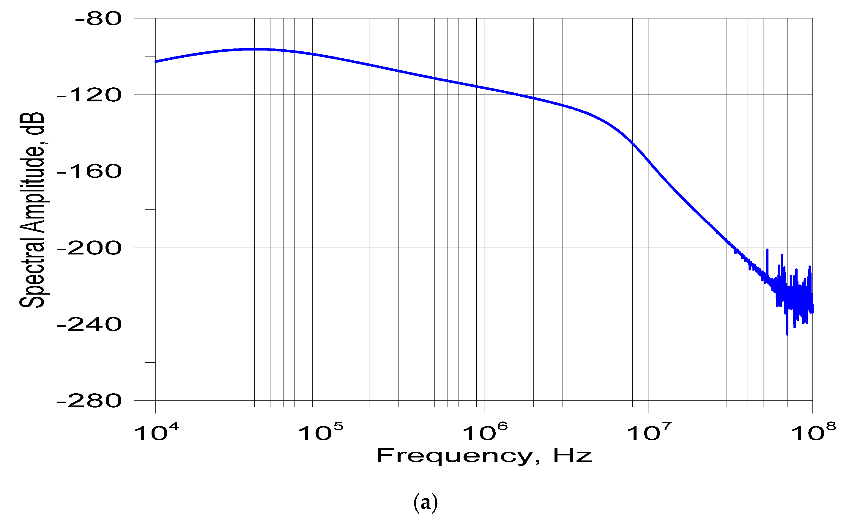
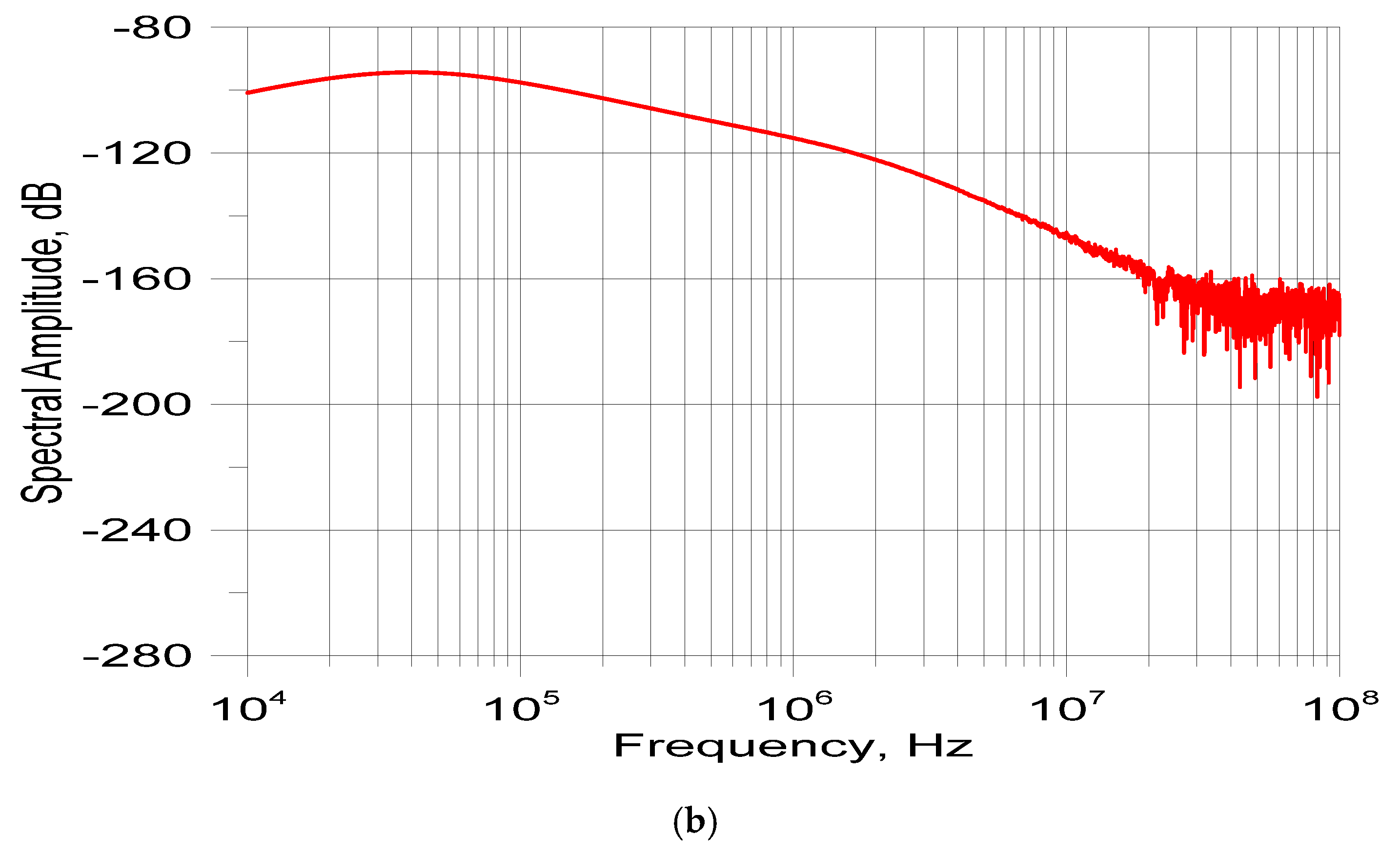
Figure 16a,b depict the frequency spectrum of the radiation field at 100 km, calculated over a perfectly conducting ground, with and without the stochastic nature of the growth curve. Observe how the stochastic nature of the streamer process gives rise to a significant frequency content beyond about 106 Hz.
7.6. Field Signature as a Function of the Distance
So far, we have studied the effect of various parameters of the streamer burst on the radiation field generated by CIDs. Not much information is available on the field signatures of CIDs measured close to their point of origin, but references [39,40] provide a few examples. These examples show the presence of a static field in the close signature of the NBP. The polarity of this static field is opposite to that of the initial peak of the radiation field. On the other hand, the results obtained by Leal et al. [8] show that, even up to a distance of about 10 km, the NBPs do not show a significant electrostatic field.
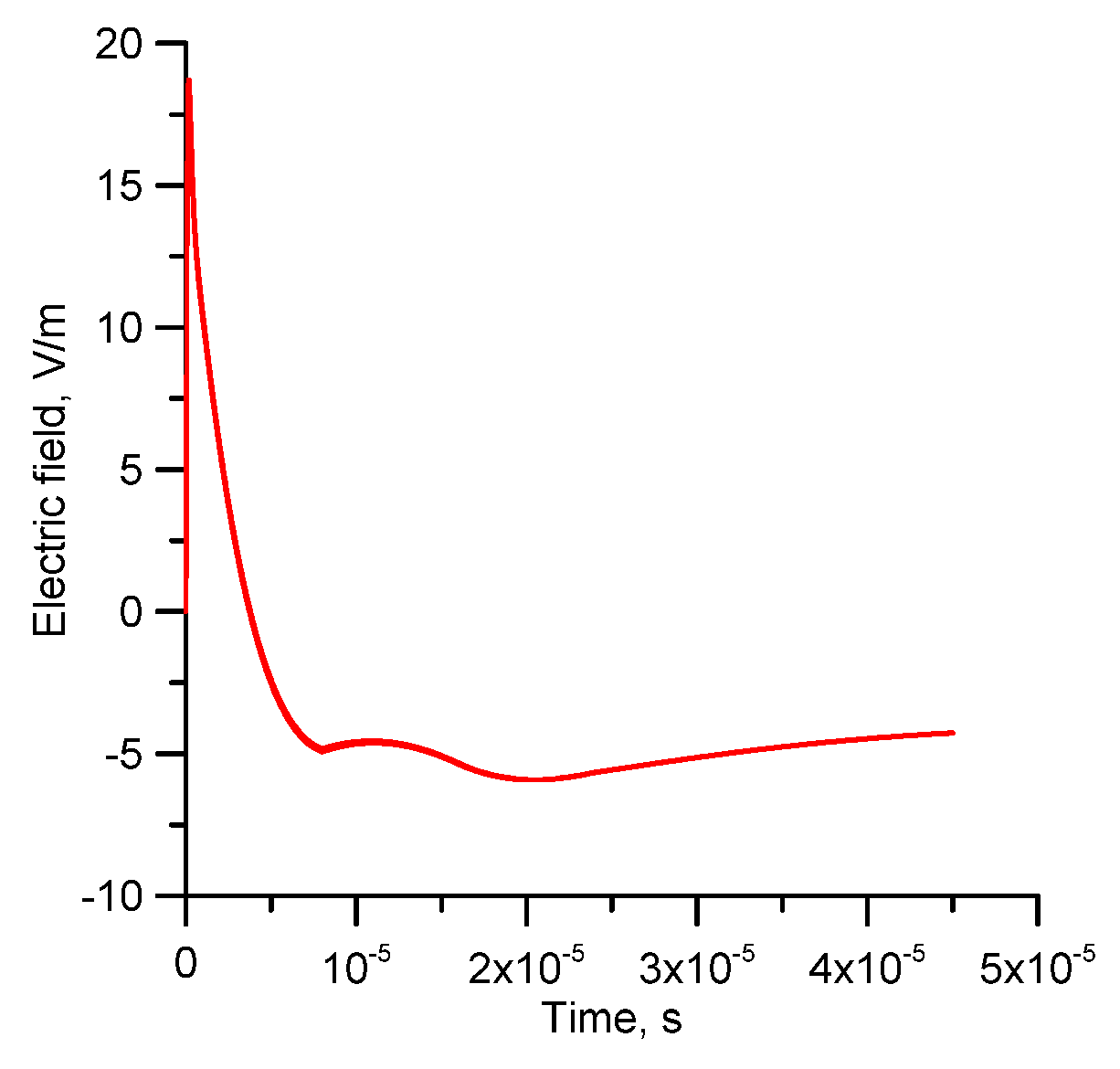
Figure 17a depicts the electric field at 10 km for the example where the corresponding radiation field is shown in Figure 8b. Note that one cannot discern a significant static field in this example. Figure 17b depicts the same example but now at a distance of 5 km. Note that there is a recognizable static step in this example. The magnitude of the static field at a given distance depends on the amount of charge displaced in the CID. Since the charge displaced by CIDs increases with the duration of the NBP, one would expect the static field at a given distance to increase as the duration of the CID increases. This can be observed from Figure 17c, where the electric field at 5 km distance is depicted for a CID with = 8 μs. Note that the field does not reach to zero level due to the presence of the static field.
Figure 18 shows the same example of Figure 17c but with the speed increased from 3 × 10⁷ m/s to 6 × 10⁷ m/s. Again, the peak amplitude at 100 km is normalized to 10 V/m. Observe also that the magnitude of the opposite overshoot of the close field, which is generated mostly by the velocity field, decreases as the speed of the streamers increases. The reason for this is the reduction of the velocity field as the streamer speed increases. This is caused by the factor present in the field equations pertinent to the velocity field. Actually, the velocity field goes to zero as the speed of propagation of the streamers reaches the speed of light. Note that the static field has a polarity opposite to that of the initial radiation field. This feature is in agreement with the experimental data presented in [39,40].
8. Discussion
In the results presented here, we have treated the CID as a normal streamer burst and the NBP as the radiation generated by the streamer burst. Let us discuss here the various questions that will arise from this assumption.
8.1. Streamer Initiation
As outlined previously, streamer initiation is preceded by electron avalanches, and this indicates that the electric field has to increase beyond the breakdown electric field over a length of space, called the critical avalanche length, so that the avalanche can be converted into a streamer. The critical avalanche length decreases with increasing electric field. For example, if the field is uniform and just above the breakdown electric field in atmospheric pressure, the critical avalanche length will be about 1–10 cm. Once a streamer is initiated, it will continue to propagate in the background electric field if the latter remains above a certain threshold. However, how this background electric field that is large enough to initiate and maintain the propagation of streamers is generated from the cloud particles is a question that has not yet been answered by the atmospheric electricity community. One possibility is the local increase of the electric field by cloud particles [41,42]. Another possibility is the stochastic nature of the air turbulence inside the cloud that will compress the cloud particles into a smaller volume momentarily, thus increasing the electric field and giving rise to the generation of streamers from a collection of cloud particles [43,44]. The third possibility is the development of regions of high electric fields due to the action of relativistic avalanches [45]. We assume that CIDs are initiated by a process unknown to us or perhaps by a process similar to the ones described above.
8.2. Thermalization
The difference between CID and the streamer bursts taking place under normal atmospheric conditions is the apparent lack of a hot conducting channel associated with the CID. At atmospheric pressure, charges as small as several micro-coulombs flowing through a single channel are capable of heating the channel [30,33]. Of course, a single streamer channel is a cold discharge and its current is not large enough to heat the streamer channel. However, the accumulated current and the charge associated with all the streamers passing through the common stem are large enough to heat the stem and give rise to a hot channel section. Even in a CID, it is doubtful whether a single streamer channel can give rise to a conducting channel section. As in the case of laboratory discharges, the charge and current from a large number of streamers have to pass through a common stem or channel section in order to create a hot channel in a CID. The reason, for the apparent absence of a hot channel, if a CID is a pure streamer burst, could be due to the low air pressure in the region under consideration. Let us consider the physical processes which lead to the heating of the channel. The heating of the channel takes place when the neutral particles and ions gain enough energy so that thermal ionization becomes effective. This process requires effective transfer of energy from electrons to ions and neutrals. Certain conditions have to be satisfied before this energy transfer can take place and the process through which this effective energy transfer from electrons to neutrals is achieved is called the thermalization. Let us consider this process in more detail [46].
In the streamer phase (or cold phase) of the discharge, many free electrons are lost due to attachment to electronegative Oxygen. Furthermore, a considerable amount of energy gained by electrons from the electric field is used in exciting molecular vibrations. Since the electrons can transfer only a small fraction of their energy to neutral atoms during elastic collisions, the electrons have a higher temperature than the neutrals. That is, the gas and the electrons are not in thermal equilibrium. As the gas temperature rises to about 1600–2000 K, rapid detachment of the electrons from negative Oxygen ions supplies the discharge with a copious amount of electrons, thus enhancing the ionization. As the temperature rises, the Vibration–Translation relaxation time decreases and the vibrational energy converts back to translational energy, thus accelerating the heating process. As the ionization process continues, the electron density in the channel continues to increase. When the electron density increases to about 1017 cm−3, a new process starts in the discharge channel. This is the strong interaction of electrons with positive ions through long range Coulomb forces. The Coulomb interaction leads to a rapid transfer of the energy of electrons to positive ions causing the electron temperature to decrease and the temperature of the positive ions to increase. The positive ions, having the same mass as the neutrals, transfer their energy to neutrals very quickly, in a time on the order of 10−8 s. This process is called thermalization. The transfer of energy from the electrons to the ions and neutrals during the thermalization process results in a rapid heating of the gas. At this stage, the thermal ionization sets in causing a rapid increase in the ionization and the conductivity of the channel. The rapid increase in the conductivity of the channel leads to an increase in the current in the discharge channel and the collapse of the applied voltage leading to a spark. During thermalization, as the electron temperature decreases, the gas temperature increases and very quickly all the components of the discharge, namely electrons, ions, and neutrals, will achieve the same temperature and the discharge will reach local thermodynamic equilibrium.
As outlined above, the thermalization requires electron densities of about 1017 electrons per cubic centimeter. At atmospheric pressure, there are about 2.68 × 10¹⁹ neutral particles per cubic centimeter and, in order to reach electron densities on the order of 1017 per cubic centimeter, the level of ionization has to be about 0.01. Immediately after thermalization, the electron density in the discharge channel may reach values about 1018 cm−3 thanks to the contribution of thermal ionization. This corresponds to about 0.1 level of ionization. At low air density corresponding to height of 10 km or more, in order to create 1017 cm−3 necessary for thermalization, the ionization level of air has to reach a value close to 0.1. It is doubtful whether such level of ionization can be reached in the discharge channel purely due to electron collisions without the support of thermal ionization. This fact may be the reason for the absence of hot channels in CIDs. Another reason that may contribute to the lack of a thermal channel in CIDs could be the following. The charge transported by CIDs lie in the range of 0.5 to 1C. It is possible that the region of this charge transport is distributed over a large cloud volume decreasing the possibility of channel thermalization. Thus, the higher the altitude of the origin of CIDs, the more difficult the creation of a thermalized channel by the streamer burst would be.
However, if a CID-like discharge takes place at lower altitudes where the air density is high, it may directly lead to a thermalized channel and, instead of giving rise to a CID, it may indeed give rise to a hot channel leading to a lightning flash. This is the case because, at higher pressures, the higher particle density could aid in generating the electron densities on the order of 1017 cm−3 necessary for the thermalization and subsequent heating of the channel. Moreover, at lower altitudes, the spatial extent of the source region generating the streamer bursts would be restricted by this thermalization process. This is the case because, when the stem of streamer channels first becomes thermalized, it would start growing rapidly due to the field enhancement at its tip while transporting opposite charge rapidly into the source region. This will reduce the electric field in the source region and clamp down on the growth of streamers from the other regions. This is exactly what is observed in the laboratory. Even though a large number of streamer bursts may start from the electrode, only one will be thermalized and give rise to a leader discharge while the others die down. Thus, a CID-type streamer burst taking place at higher air densities may directly give rise to a leader and dampen the growth of other streamers from the source region, leading to a lightning discharge. Thus, the streamer burst associated with the initiation of the leader may contain much less charge, and its electric field signature would be weak in comparison to a NBP. These could be the reasons why NBPs are rarely observed in Sweden, where the charge centers are located at low altitudes, but are a very frequent feature in tropical thunderstorms. Since the thermalization of air becomes more probable during streamer bursts in regions of high pressure, a streamer burst that originates in Swedish thunderclouds may end up more often as a lightning event than a CID. Furthermore, Electric fields in thunderclouds have been estimated to be of the order of 100 kV/m. The background electric field necessary for streamer propagation at 8–10 km height is close to or less than this value. Thus, if streamers are initiated by local enhancement of the electric field, they will be able to propagate long distances in the background electric field. In regions of high air density, however, one needs a higher electric field for streamer propagation and the chances that streamer bursts can propagate long distances become rarer. This again could also be a possible explanation for the lack of CIDs in Swedish thunderstorms. Of course, in between these two extreme situations, i.e., streamer bursts leading either to lightning flashes (at low altitudes) or CIDs (at high altitudes), there could be cases where a CID would give rise to a lightning discharge occasionally (at mid altitudes) if the charge associated with the CID is large enough. Moreover, it is also possible that the CIDs are generated during the charging stage of the storms and, even if a thermal channel is produced, the background conditions may not be suitable for the initiation of lightning flashes.
It is important to point out that a single streamer is a cold discharge, and it is not capable of giving rise to a hot channel. In laboratory discharges the heating takes place at a common streamer stem through which the accumulated current and charge from a large number of streamers are passing. The situation could be the same in the streamer discharges that develop inside the clouds and, whenever hot channels are generated inside clouds by streamer systems, it is probably achieved at the common streamer stems.
8.3. Streamer Speed
At standard atmospheric pressure, the streamer propagates at maximum speeds of about 5 × 10⁶ m/s. Not much information is available on the speed of streamers at low pressures. The similarity laws predict that the streamer speeds should not depend on the atmospheric pressure. On the other hand, the cloud environment consists of a large number of cloud particles of various dimensions. The particle density increases with decreasing radii of the particles. For example, in mature clouds, the number of particles may increase to several hundred per cubic meter. As the streamer front propagates, it generates a high electric field ahead of it. As the number of streamer heads intensifies, the streamer front appears as a charged sheet and the electric field extends over a significant distance in front of the streamer system. This electric field could be large enough to generate streamers from the cloud particles located ahead of the streamer front and in principle the streamer front can travel with the speed of light, the speed at which the electric field extends in front of the streamer front. However, in reality, the speed will be less than the speed of light. This could be the case because, for efficient propagation, the charge in the negative streamers generated by the particles towards the forward moving streamer front has to be neutralized quickly by the positive streamers associated with the streamer front. Otherwise, the electric field in front of the streamer system will be reduced. Thus, the speed of the streamer system is somewhat reduced by the finite time necessary for this charge neutralization. This particle assisted propagation (depicted in Figure 19) could be a reason for the fast propagation of streamers inside the cloud environment.
8.4. A final Comment
In a recent paper Cooray et al. [14] showed that main features of NBPs can be explained by treating CIDs as a series of relativistic avalanches. Here we have shown that the features of NBPs can be explained by treating CIDs as a streamer burst. Further experimental data are needed to find out whether all the electromagnetic emissions from thunderclouds having features similar to those of NBPs are generated by streamer bursts or whether some of them are generated by relativistic avalanches. Moreover, the possibility that some of the NBPs could be a result of combined streamer bursts and relativistic avalanches has also to be investigated.
9. Conclusions
In this paper, we have studied the features of CIDs assuming that they consist of streamer bursts without any conducting channels. A typical CID may contain about 109 streamer heads during the time of its maximum growth. A CID consists of a current front of several nanosecond duration that travels forward with the speed of the streamers. The amplitude of this current front increases initially during the streamer growth and decays subsequently as the streamer burst continues to propagate. Depending on the conductivity of the streamer channels, there could be a low-level current flow behind this current front which transports negative charge towards the streamer origin.
The features of the current associated with the CID are very different from the radiation field that it generates. The duration of the radiation field of a CID is about 10–20 μs, whereas the duration of the propagating current pulse associated with the CID is no more than a few nanoseconds. The peak current of a CID is the result of a multitude of small currents associated with a large number of streamers. If all the forward moving streamer heads lie in a single horizontal plane, according to the simulations the cumulative current that radiates at its peak value could be about 108 A. However, the current associated with an individual streamer is no more than a few hundreds of mA. If the location of the forward moving streamer heads are spread along a vertical direction, the peak current will be reduced considerably. Moreover, this large current is spread over an horizontal area of several tens to several hundreds of square meters.
The streamer model of the CID could explain the fine structure of the radiation fields present both in the electric field and electric field time derivative.
One important feature of the model is that, once the distant radiation field generated by a CID is measured, the model can be used to obtain information on how the number of streamers in the streamer burst varies in time. This is the case because the temporal variation of the streamer growth curve is proportional to the time integral of the radiation field. If the speed of development of the streamer burst is available, the spatial growth of the streamer burst can also be obtained.
Author Contributions
V.C. and G.C. conceived the idea and developed the mathematics and the computer software. All authors contributed equally in the analysis and in writing the paper. All authors have read and agreed to the published version of the manuscript.
Funding
This work was supported by Swedish Research Council grant VR-2015-05026 and partly by the fund from the B. John F. and Svea Andersson donation at Uppsala University.
Conflicts of Interest
The authors declare no conflict of interest.
References
- Le Vine, D.M. Sources of the strongest RF radiation from lightning. J. Geophys. Res. 1980, 85, 4091. [Google Scholar] [CrossRef] [Green Version]
- Willett, J.C.; Bailey, J.C.; Krider, E.P. A class of unusual lightning electric field waveforms with very strong high-frequency radiation. J. Geophys. Res. 1989, 94, 16255. [Google Scholar] [CrossRef]
- Smith, D.A.; Shao, X.M.; Holden, D.N.; Rhodes, C.T.; Brook, M.; Krehbiel, P.R.; Stanley, M.; Rison, W.; Thomas, R.J. A distinct class of isolated intracloud lightning discharges and their associated radio emissions. J. Geophys. Res. Atmos. 1999, 104, 4189–4212. [Google Scholar] [CrossRef]
- Nag, A.; Rakov, V.A.; Tsalikis, D.; Cramer, J.A. On phenomenology of compact intracloud lightning discharges. J. Geophys. Res. 2010, 115, D14115. [Google Scholar] [CrossRef] [Green Version]
- Nag, A.; Rakov, V.A. Compact intracloud lightning discharges: 1. Mechanism of electromagnetic radiation and modeling. J. Geophys. Res. Atmos. 2010, 115. [Google Scholar] [CrossRef] [Green Version]
- Karunarathne, S.; Marshall, T.C.; Stolzenburg, M.; Karunarathna, N. Observations of positive narrow bipolar pulses. J. Geophys. Res. Atmos. 2015, 120, 7128–7143. [Google Scholar] [CrossRef]
- Bandara, S.; Marshall, T.; Karunarathne, S.; Stolzenburg, M. Electric field change and VHF waveforms of Positive Narrow Bipolar Events in Mississippi thunderstorms. Atmos. Res. 2020, 243, 105000. [Google Scholar] [CrossRef]
- Leal, A.F.R.; Rakov, V.A.; da Rocha, B.R.P. Classification of CIDs observed in Florida using the Lightning Detection and Waveform Storage System (LDWSS). In Proceedings of the International Symposium on Lightning Protection (XIV SIPDA), Natal, Brazil, 2–6 October 2017. [Google Scholar]
- Cooray, V.; Lundquist, S. Characteristics of the radiation fields from lightning in Sri Lanka in the tropics. J. Geophys. Res. 1985, 90, 6099–6109. [Google Scholar] [CrossRef]
- Sharma, S.R.; Fernando, M.; Cooray, V. Narrow positive bipolar radiation from lightning observed in Sri Lanka. J. Atmos. Sol. Terr. Phys. 2008, 70, 1251–1260. [Google Scholar] [CrossRef]
- Gunasekara, L.; Fernando, M.; Sonnadara, U.; Cooray, V. Characteristics of Narrow Bipolar Pulses observed from lightning in Sri Lanka. J. Atmos. Solar Terr. Phys. 2016, 138–139, 66–73. [Google Scholar] [CrossRef]
- Ahmad, N.A.; Fernando, M.; Baharudin, Z.A.; Cooray, V.; Ahmad, H.; Abdul Malek, Z. Characteristics of narrow bipolar pulses observed in Malaysia. J. Atmos. Sol. Terr. Phys. 2010, 72, 534–540. [Google Scholar] [CrossRef]
- Ahmad, M.R.; Esa, M.R.M.; Cooray, V.; Baharudin, Z.A.; Hettiarachchi, P. Latitude dependence of narrow bipolar pulse emissions. J. Atmos. Solar Terr. Phys. 2015, 128, 40–45. [Google Scholar] [CrossRef]
- Cooray, V.; Cooray, G.; Marshall, T.; Arabshahi, S.; Dwyer, J.; Rassoul, H. Electromagnetic fields of a relativistic electron avalanche with special attention to the origin of lightning signatures known as narrow bipolar pulses. Atmos. Res. 2014, 149, 346–358. [Google Scholar] [CrossRef]
- Cooray, V.; Fernando, M.; Gunasekara, L.; Nanayakkara, S. Effects of Propagation of Narrow Bipolar Pulses, Generated by Compact Cloud Discharges, over Finitely Conducting Ground. Atmosphere 2018, 9, 193. [Google Scholar] [CrossRef] [Green Version]
- Wu, T.; Dong, W.; Zhang, Z.; Funaki, T.; Yoshida, S.; Morimoto, T.; Ushio, T.; Kawasaki, Z. Discharge height of lightning narrow bipolar events. J. Geophys. Res. Atmos. 2012, 117. [Google Scholar] [CrossRef]
- Leal, A.R.F.; Rakov, V.A.; Rocha, B.R.P. Estimation of ionospheric reflection heights using CG and IC lightning electric field waveforms. In Proceedings of the International Symposium on Lightning Protection (XIV SIPDA), Natal, Brazil, 2–6 October 2017. [Google Scholar]
- Krehbiel, P.; da Silva, C.; Cummer, S. Continued mysteries of lightning studies. In Proceedings of the 16th International Conference on Atmospheric Electricity, Nara, Japan, 17–22 June 2018. [Google Scholar]
- Gurevich, A.V.; Medvedev, Y.V.; Zybin, K.P. New type discharge generated in thunderclouds by joint action of runaway breakdown and extensive atmospheric shower. Phys. Lett. A 2004, 329, 348–361. [Google Scholar] [CrossRef]
- Gurevich, A.V.; Zybin, K.P. Runaway Breakdown and the Mysteries of Lightning. Phys. Today 2005, 58, 37–43. [Google Scholar] [CrossRef] [Green Version]
- Marshall, T.C.; Watson, S.S. Current propagation model for a narrow bipolar pulse. Geophys. Res. Lett. 2007, 34. [Google Scholar] [CrossRef]
- Babich, P.; Bochkov, E.I.; Kutsyk, I.M. Numerical simulation of compact intracloud discharge and generated electromagnetic pulse. Dokl. Earth Sci. 2015, 462, 569–599. [Google Scholar] [CrossRef]
- Rison, W.; Krehbiel, P.R.; Stock, M.G.; Edens, H.E.; Shao, X.-M.; Thomas, R.J.; Stanley, M.A.; Zhang, Y. Observations of narrow bipolar events reveal how lightning is initiated in thunderstorms. Nat. Commun. 2016, 7, 10721. [Google Scholar] [CrossRef] [Green Version]
- Tilles, J.N.; Liu, N.; Stanley, M.A.; Krehbiel, P.R.; Rison, W.; Stock, M.G.; Dwyer, J.R.; Brown, R.; Wilson, J. Fast negative breakdown in thunderstorms. Nat. Commun. 2019, 10, 1648. [Google Scholar] [CrossRef] [PubMed] [Green Version]
- Iudin, I.; Davydenko, S.S. Fractal model of a compact intracloud discharge. I. Features of the structure and evolution. Radiophys. Quantum Electron. 2015, 58, 477–496. [Google Scholar] [CrossRef]
- Davydenko, S.S.; Iudin, D.I. Fractal model of a compact intracloud discharge. II. Specific features of electromagnetic emission. Radiophys. Quantum Electron. 2016, 59, 560–575. [Google Scholar] [CrossRef]
- Attanasio, A.; Krehbiel, P.R.; da Silva, C.L. Griffiths and Phelps Lightning Initiation Model, Revisited. J. Geophys. Res. 2019. [Google Scholar] [CrossRef]
- Liu, N.; Dwyer, J.R.; Tilles, J.N.; Stanley, M.A.; Krehbiel, P.R.; Rison, W.; Brown, R.G.; Wilson, J.G. Understanding the radio spectrum of thunderstorm narrow bipolar events. J. Geophys. Res. 2019. [Google Scholar] [CrossRef]
- Griffiths, R.F.; Phelps, C.T. A model for lightning initiation arising from positive corona streamer development. J. Geophys. Res. 1976, 81, 3671–3676. [Google Scholar] [CrossRef]
- Gallimberti, I. The mechanism of long spark formation. J. Phys. Colloq. 1979, 40, 193–249. [Google Scholar] [CrossRef]
- Briels, T.M.P.; Kos, J.; Winands, G.J.J.; van Veldhuizen, E.M.; Ebert, U. Positive and negative streamers in ambient air: measuring diameter, velocity and dissipated energy. J. Phys. D Appl. Phys. 2008, 41, 234004. [Google Scholar] [CrossRef] [Green Version]
- Briels, T.M.P.; van Veldhuizen, E.M.; Ebert, U. Positive streamers in air and nitrogen of varying density: experiments on similarity laws. J. Phys. D Appl. Phys. 2008, 41, 234008. [Google Scholar] [CrossRef] [Green Version]
- Les Renardières Group, L.R. Research on long gap discharges at Les Renardières. Electra 1972, 23, 53–157. [Google Scholar]
- Aleksandrov, N.L.; Bazelyan, E.M. Temperature and density effects on the properties of long positive streamer in air. J. Phys. D Appl. Phys. 1996, 29, 2873–2880. [Google Scholar] [CrossRef]
- Pasco, P.V. Theoretical modeling of sprites and jets. In Sprites, Elves and Intense Lightning Discharges; Füllekrug, M., Mareev, E., Rycroft, M.J., Eds.; Nato Science Series; Springer: Dordrecht, The Netherlands, 2006. [Google Scholar]
- Cooray, V.; Cooray, G. The Electromagnetic Fields of an Accelerating Charge: Applications in Lightning Return-Stroke Models. IEEE Trans. Electromagn. Compat. 2010, 52, 944–955. [Google Scholar] [CrossRef]
- Cooray, G.; Cooray, V. Electromagnetic fields of a short electric dipole in free space—Revisited. Prog. Electromagn. Res. Lett. 2012, 131, 357–373. [Google Scholar] [CrossRef] [Green Version]
- Cooray, V.; Cooray, G.; Rubinstein, M.; Rachidi, F. Generalized Electric Field Equations of a Time-Varying Current Distribution Based on the Electromagnetic Fields of Moving and Accelerating Charges. Atmosphere 2019, 10, 367. [Google Scholar] [CrossRef] [Green Version]
- Eack, K.B. Electrical characteristics of narrow bipolar events, Geophys. Res. Lett. 2004, 31, L20102. [Google Scholar] [CrossRef]
- Karunarathne, S.; Marshall, T.C.; Stolzenburg, M.; Karunarathna, N. Electrostatic field changes and durations of narrow bipolar events. J. Geophys. Res. Atmos. 2016, 121, 10–61. [Google Scholar] [CrossRef]
- Sadighi, S.; Liu, N.; Dwyer, J.R.; Rassoul, H.K. Streamer formation and branching from model hydrometeors in subbreakdown conditions inside thunderclouds. J. Geophys. Res. Atmos. 2015, 120, 3660–3678. [Google Scholar] [CrossRef]
- Babich, L.P.; Bochkov, E.I.; Neubert, T. The role of charged ice hydrometeors in lightning initiation. J. Atmos. Solar Terr. Phys. 2017, 154, 43–46. [Google Scholar] [CrossRef]
- Köhn, C.; Chanrion, O.; Neubert, T. HighEnergy Emissions Induced by Air Density Fluctuations of Discharges. Geophys. Res. Lett. 2018, 10, 5194–5203. [Google Scholar] [CrossRef]
- Dubinova, A.; Rutjes, C.; Ebert, U.; Buitink, S.; Scholten, O.; Trinh, G.T. Prediction of lightning inception by large ice particles and extensive air showers. Phys. Rev. Lett. 2015, 115, 015002. [Google Scholar] [CrossRef]
- Dwyer, J.R. The initiation of lightning by runaway air breakdown. Geophys. Res. Lett. 2005, 32, L20808. [Google Scholar] [CrossRef]
- Cooray, V. Mechanism of Electrical Discharges. In The Lightning Flash, 2nd ed.; Cooray, V., Ed.; IETPublishers: London, UK, 2014. [Google Scholar]
Figure 1.
Waveshapes of narrow bipolar pulses measured in the study conducted by Karunarathne et al. [6] and summarized in Bandara et al. [7]. (a) Example of a type A NBP, (b) example of a type B NBP, (c) example of a Type C NBP and (d) example of a type D NBP as defined in [6,7]—figure obtained from [7].

Figure 2.
Two examples of the time derivative of NBPs (Narrow Bipolar Pulses) observed in the study conducted by Gunasekara et al. [11]. Note that the vertical scale is in arbitrary units.
Figure 2.
Two examples of the time derivative of NBPs (Narrow Bipolar Pulses) observed in the study conducted by Gunasekara et al. [11]. Note that the vertical scale is in arbitrary units.

Figure 3.
Schematic representation of the propagation of a streamer. In the diagram, the effects of multiple avalanches traveling towards the streamer head is represented by an equivalent avalanche. Adapted from [30]. As the charge on the head of the streamer is neutralized by the incoming avalanche, the streamer extends forward by a length equal to the diameter of the streamer channel. In the diagram, is the number of positive ions at the head of the streamer and is the radius of the streamer channel.

Figure 4.
In the analysis, a streamer is considered as a propagating positive charge distribution (marked by red dots). As the streamer branches, new streamer heads are created and there are two possible scenarios for the fate of the resulting negative charge (represented by blue dots). (I) In this scenario, the negative charge travels towards the origin of the streamer and is accumulated there. (II) In this scenario, the negative charge remains at the same location where it is created. The arrows indicate the direction of travel of the charge distributions.

Figure 5.
The geometry pertinent to the calculation of the radiation field generated during the initiation and branching of a streamer channel.
Figure 5.
The geometry pertinent to the calculation of the radiation field generated during the initiation and branching of a streamer channel.

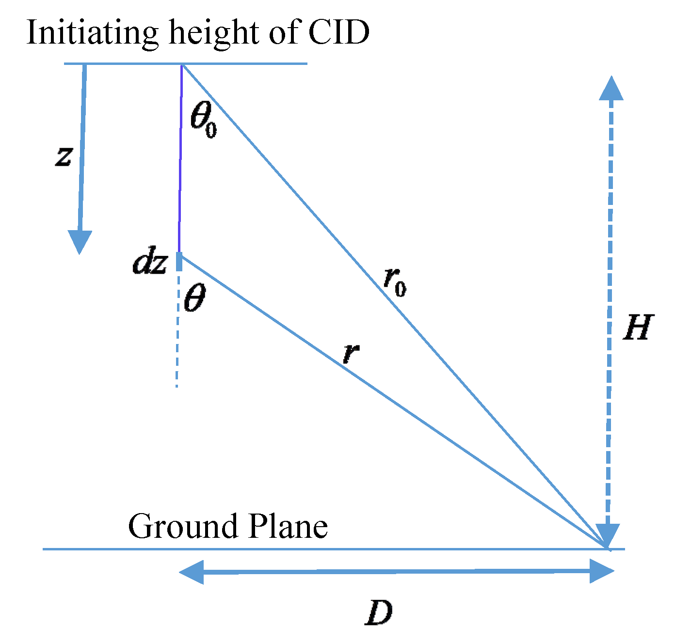
Figure 6.
Geometry relevant to the calculation of the electric field generated by the streamer burst.
Figure 6.
Geometry relevant to the calculation of the electric field generated by the streamer burst.

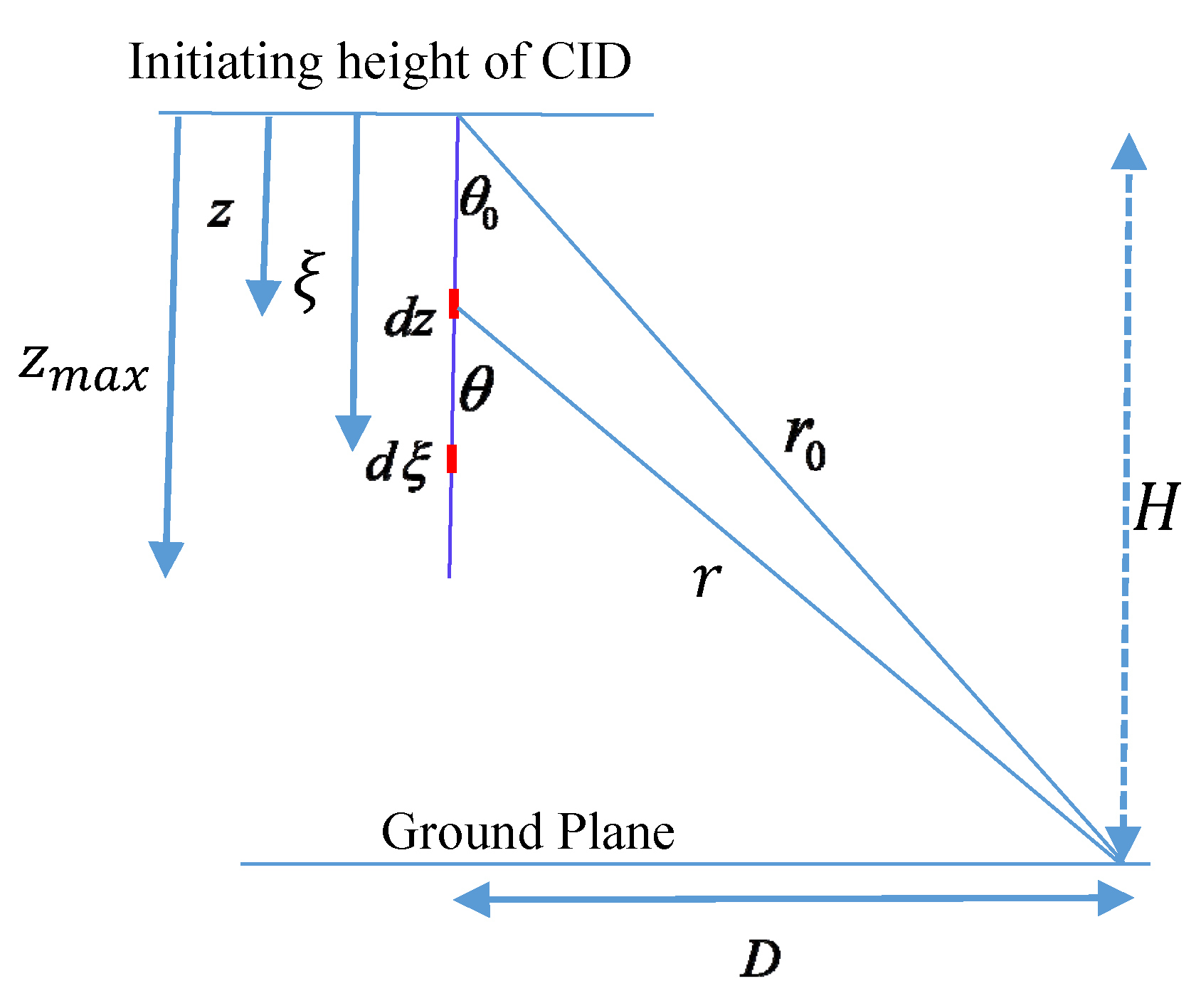
Figure 7.
Geometry necessary for the calculation of the velocity field generated by the streamer burst.
Figure 7.
Geometry necessary for the calculation of the velocity field generated by the streamer burst.

Figure 8.
NBPs calculated using the growth curve given by Equation (34). (a) electric field is calculated assuming that the negative charge remains where it is generated with = 0.1 μs, = 4.0 μs; (b) electric field is calculated assuming that the negative charge propagates backward towards the streamer origin with = 0.1 μs, = 4.0 μs and = . In both examples, the value of was selected to make the electric field normalized to 100 km equal to 10 V/m. The speed of propagation of the forward moving and backward moving current is selected to be 3 × 10⁷ m/s. The number of elementary charges at the streamer head is assumed to be 109.

Figure 9.
(a) Number of forward moving streamer heads present at a given location. Curves i and ii correspond to non-conducting and partially conducting streamer channels; (b) number of newly created streamer heads as a function of distance from the origin; (c) peak current (sum of the currents associated with the forward moving streamer heads) associated with the forward moving front of the streamer burst corresponds to the curve i in (a). Curves i and ii correspond to non-conducting and partially conducting streamer channels.

Figure 10.
The lateral growth of the streamer burst as a function of distance obtained for the two cases (a) and (b) presented in Figure 8.
Figure 10.
The lateral growth of the streamer burst as a function of distance obtained for the two cases (a) and (b) presented in Figure 8.

Figure 11.
The charge deposited in space ahead of the origin of the streamer burst. (a) non conducting streamer channel where the negative charge remains where it is created; (b) partially conducting streamer channel where the negative charge is transported back to the streamer origin. The parameters used in the calculation are identical to those used to obtain Figure 8a,b.

Figure 12.
The effect of increasing the duration of the backward moving electron current. (a) = 1 μs; (b) = 3 μs; (c) = 7.5 μs. The rest of the parameters are identical to those of Figure 8b.
Figure 12.
The effect of increasing the duration of the backward moving electron current. (a) = 1 μs; (b) = 3 μs; (c) = 7.5 μs. The rest of the parameters are identical to those of Figure 8b.

Figure 13.
The effect of multiple streamer bursts arising from the same origin on the NBP. In the simulation, the growth parameters of each streamer burst is assumed identical to the one used previously except that the value of was selected to make the peak of the NBP equal to 10 V/m at 100 km. (a) separation between streamer bursts 1.0 μs; (b) separation between streamer bursts 1.5 μs.

Figure 14.
(a) Electric radiation field at 100 km without taking into account the randomness of the growth curve; (b) electric radiation field at 100 km taking into account the randomness of the growth curve.
Figure 14.
(a) Electric radiation field at 100 km without taking into account the randomness of the growth curve; (b) electric radiation field at 100 km taking into account the randomness of the growth curve.

Figure 15.
(a) Electric field time derivative without taking into account the randomness of the growth curve; (b) electric field time derivative taking into account the randomness of the growth curve; (c) (d) and (e) electric field derivatives measured with apparatus having risetimes of 1 ns, 5 ns, and 10 ns, respectively.

Figure 16.
(a) Frequency spectrum of the radiation field without taking into account the randomness of the streamer breakdown. The spectra were range normalized so that 0 dB corresponds to 1 (V/m/Hz) at 100 km; (b) frequency spectrum of the radiation field including the randomness of the streamer breakdown. The spectra were range normalized so that 0 dB corresponds to 1 (V/m/Hz) at 100 km.


Figure 17.
(a) Electric field at 10 km corresponding to the example shown in Figure 8b; (b) electric field at 5 km corresponding to the example shown in Figure 8b; (c) electric field at 5 km when the decay time constant of the growth curve is increased from 4 μs to 8 μs.

Figure 18.
The same example as in Figure 17c but with the speed of propagation increased to 6 × 10⁷ m/s. Note that, in this example too, the peak value at 100 km is selected to be 10 V/m. Since the peak of the radiation field increases linearly with the speed of propagation, the value of had to be reduced by half compared to Figure 17c to keep the peak radiation field at 10 V/m.

Figure 19.
Schematic representation of the cloud particle assisted streamer propagation. As the streamer front moves, the electric field ahead of the streamer front causes the cloud particles located ahead of the streamer front to generate bi-directional streamers (frame to the left). The positive component of the bidirectional streamers will propagate ahead as the new front of the streamer burst while the negative counterpart of the bidirectional streamer neutralizes the positive charge of the previous front (frame to the right). The process is repeated continuously allowing the streamer burst to move rapidly.

© 2020 by the authors. Licensee MDPI, Basel, Switzerland. This article is an open access article distributed under the terms and conditions of the Creative Commons Attribution (CC BY) license (http://creativecommons.org/licenses/by/4.0/).
Share and Cite
MDPI and ACS Style
Cooray, V.; Cooray, G.; Rubinstein, M.; Rachidi, F. Modeling Compact Intracloud Discharge (CID) as a Streamer Burst. Atmosphere 2020, 11, 549. https://doi.org/10.3390/atmos11050549
AMA Style
Cooray V, Cooray G, Rubinstein M, Rachidi F. Modeling Compact Intracloud Discharge (CID) as a Streamer Burst. Atmosphere. 2020; 11(5):549. https://doi.org/10.3390/atmos11050549
Chicago/Turabian StyleCooray, Vernon, Gerald Cooray, Marcos Rubinstein, and Farhad Rachidi. 2020. "Modeling Compact Intracloud Discharge (CID) as a Streamer Burst" Atmosphere 11, no. 5: 549. https://doi.org/10.3390/atmos11050549
Note that from the first issue of 2016, this journal uses article numbers instead of page numbers. See further details here.