
Abstract
Two synthetic diagnostics are implemented for the high-k scattering system in NSTX (Smith et al 2008 Rev. Sci. Instrum. 79 123501) allowing direct comparisons between the synthetic and experimentally detected frequency and wavenumber spectra of electron-scale turbulence fluctuations. Synthetic diagnostics are formulated in real-space and in wavenumber space, and are deployed in realistic electron-scale simulations carried out with the GYRO code (Candy and Waltz 2003 J. Comput. Phys. 186 545). A highly unstable electron temperature gradient (ETG) mode regime in a modest-β NSTX NBI-heated H-mode discharge is chosen for the analysis. Mapping the measured wavenumbers to field aligned coordinates shows that the high-k system is sensitive to fluctuations that are closer to the spectral peak in the density fluctuation wavenumber spectrum (streamers) than originally predicted. The analyses of synthetic spectra show that the frequency response of the detected fluctuations is dominated by Doppler shift and is insensitive to the turbulence drive. The shape of the high-k density fluctuation wavenumber spectrum is sensitive to the ETG turbulence drive conditions, and can be reproduced in a sensitivity scan of the most pertinent turbulent drive terms in the simulation.
Export citation and abstract BibTeX RIS
1. Introduction
Plasma turbulence gives rise to anomalous transport of particles and heat in magnetic confinement fusion devices [1], which is detrimental to confinement. The complex, kinetic nature of the turbulence has led to the development of sophisticated gyrokinetic models implemented in state-of-the-art numerical simulations [2] (non-linear gyrokinetic simulation) to study the turbulence and consequent turbulence-driven transport. The gyrokinetic model requires extensive validation in today's fusion experiments before achieving a predictive capability for future fusion devices such as ITER [3], FNSF [4] and beyond. Confidence in the predictions from gyrokinetic simulations can be gained via a thorough validation process, which should include detailed comparisons of turbulence characteristics in addition to the traditional comparisons of turbulent fluxes [5, 6]. In this article we make direct comparisons of density fluctuation spectra between experimental turbulence measurements by high-k scattering and non-linear gyrokinetic simulations, which are part of an extensive validation study of electron thermal transport in NSTX [7].
Turbulence in the tokamak core can live at ion gyro radius scales ( ) and at electron gyro radius scales (
 ), where
  is the perpendicular wavenumber of the turbulence and
  is the ion sound gyro radius evaluated at the ion sound speed
  , and
, and  is the ion gyro-frequency. Experimentally, coherent scattering techniques implemented through Doppler backscattering (DBS) [8–16] and high-k scattering [17–33] can probe turbulent density fluctuations at electron-scales
  . These can be of special importance in spherical tokamak plasmas where electron thermal transport dominates heat transport losses in H-mode scenarios [34–39], and electron-scale turbulence can be the main heat loss mechanism in some operating regimes [40, 41]. Previous work to validate non-linear electron-scale gyrokinetic simulations against experimental turbulence measurements has focused on establishing qualitative turbulence comparisons, with more recent efforts expanding to quantitative comparisons through synthetic diagnostic development [42–46]. However, the challenge remains to achieve direct quantitative comparisons of the high-k frequency and wavenumber turbulent fluctuation spectrum between experiment and simulation.
Coherent scattering diagnostics are sensitive to a specific wavenumber  of the turbulent fluctuations. As a result, previous synthetic diagnostic work has been formulated in wavenumber space (k-space), via the selection of
  by use of a filter in wavenumber space [42–46]. However, the scattering signal for coherent scattering is fundamentally calculated from first principles via integration of the electron density fluctuation amplitude in real space [47, 48]. In this article we build on past work to show how the wavenumber formulation can be naturally derived from real space. We propose two equivalent formulations, in real space and in k-space, for the computation of the scattering signal from coherent scattering in realistic field-aligned coordinates. The quantitative agreement shown between the real space and k-space based synthetic diagnostics provides improved confidence on the validity of the computed synthetic spectra shown in this work.
One of the difficulties in developing synthetic diagnostics for coherent scattering is the different wavenumber definitions employed in experiments and gyrokinetic codes. Experiments generally use cylindrical or Cartesian coordinates for the components of the measured wavenumber  , which are provided by ray-tracing or equivalent calculations. Gyrokinetic codes operate in field-aligned coordinates and use internal wavenumber definitions. An 'apples-to-apples' comparison between experimental turbulence measurements and simulated turbulence requires a mapping of the measured wavenumber to field-aligned coordinates, implemented as part of this work. The wavenumber mapping is also an important step in the development of synthetic diagnostics in wavenumber space. This complexity is absent in the real space formulation, but is necessary to understand the measurement wavenumber range of the diagnostic in the density fluctuation spectra. This motivates the implementation of two equivalent formulations of the synthetic diagnostic, in real space and in k-space.
The rest of this article proceeds as follows. In section 2 we discuss some theoretical considerations of coherent scattering measurements of turbulence fluctuations. In section 3 we outline the implementation of synthetic diagnostics for coherent scattering systems in realistic field-aligned tokamak geometry and introduce the wavenumber mapping. In this section we highlight the importance of geometric effects, such as the normalizing B-field, the effect of plasma elongation and Shafranov shift, which can strongly affect the interpretation of the measured wavenumber components from scattering measurements (by up to factors of ∼5 for the present NSTX case). In section 4 we apply the synthetic diagnostic to compute numerically generated synthetic spectra for the high-k scattering system in NSTX [26–28], using realistic electron-scale gyrokinetic simulations based on a modest-β NSTX NBI heated H-mode plasma. Finally, we compare synthetic high-k frequency and wavenumber spectra with experimental spectrum measurements. The main outcome of this work is the successful validation of electron-scale gyrokinetic simulations in the core-gradient region of a modest-β NSTX H-mode plasma via direct comparison with measured high-k density fluctuation spectra.
2. Theoretical considerations on coherent scattering measurements of density fluctuations
Coherent scattering from turbulence fluctuations inherently takes place in a confined region known as the scattering volume Vs, which is generally delimited by the size of the electromagnetic wave beam input in the plasma and by the magnetic field geometry. This leads one to interpret the scattering process as the integration of fluctuations in real space within the scattering volume. However, scattering measurements are usually interpreted in wavenumber space, based on the measurement of a specific turbulence wavenumber  , which is determined by the launching and receiving geometries of the electromagnetic wave beam. This leads one to interpret the scattering process as a selection of a specific wavenumber
  from the density fluctuations. In this section we show how the scattering process can be interpreted equally in real space as well as in k-space.
In the coherent scattering process, plasma electrons are exposed to an external source of electromagnetic radiation (e.g. a laser or microwave source, considered here to be a beam of radius a0). Accelerated by the incoming electric field, electrons radiate electromagnetic energy in the form of a radiation field. The expression for the scattered power per unit frequency and unit solid angle  is related to the frequency signal of density fluctuations
  by the textbook formula (appendix B)
where the subscript 'u' indicates that the density fluctuation signal has been properly filtered in the scattering process by a filter U in real space. In expression (1) dΩ is the solid angle, P0 is the incident beam power in watts, Ai is the incident beam area  ,
,  is the classical electron radius, T is the collection time,
  is the direction of scattering,
  is the direction of the scattered electric field and
  denotes an ensemble average. The incident radiation oscillating at a frequency ωi with wave-vector
  can be related to the scattered frequency ωs and wavenumber
  by the scattering matching conditions
  and
and  (Bragg condition), where ω and
  are the matching turbulence frequency and wavenumber (the contributions from the matching wave-vector
  are negligible and are ignored in this work).
In the case of DBS or Doppler reflectometry [8–10], ray-tracing or beam-tracing methods break down near the cut-off encountered by the incident electromagnetic wave, and a full-wave treatment might be necessary to accurately model the propagation of the electromagnetic wave in the plasma. Despite this, much of the work presented here could still prove useful to help interpret density fluctuation measurements using DBS in some operating regimes (e.g. the linear response regime). In the case of high-k scattering, the incident frequency is typically much higher than any other frequencies in the plasma ( ). The electromagnetic wave propagates above any cut-off and resonance in the plasma, validating the use of the ray-tracing methods employed in this work.
The quantity  in equation (1) has been Fourier decomposed from
  , which is the synthetic time signal of electron density fluctuations for the selected turbulence wavenumber
  .
.  can be formally computed in real space as well as in wavenumber space:
The real space filter U determines the shape of the scattering volume Vs from the incident and scattered beam profiles and the magnetic field geometry. The quantity  is the real electron density fluctuation field, and
  is the raw electron density fluctuation spectrum, computed from
  by Fourier analysis. W is the scattering filter in wavenumber space corresponding to the weights for each wavenumber
  , and is directly related to the Fourier transform of the scattering volume shape U (appendix B).
Equation (2) states the equivalence between the computation of the synthetic signal of fluctuations in real space and in wavenumber space. In wavenumber space, the synthetic signal is a sum over all turbulence wavenumber contributions around the detected wavenumber  , where a filter
  is applied to the wavenumber spectrum of fluctuations
  . W peaks around the measurement wave-vector
  , and down-selects a range of wavenumbers neighboring
  within the range
  (Vs is the scattering volume extent, m3). In real space, the synthetic signal can be interpreted as the Fourier component
  of the real quantity
  . As a result of U in the real integration, the scattering signal has not only contributions from one lone
  (obtained for U = 1), but also from an array of wavenumbers around
  in the range
  (
( is the spectral width of the filter
  ). Full information about the detected turbulence wavenumber
  and the spectral width
  is preserved in the computation of
  according to both formulations, and motivates their implementation for realistic tokamak scattering experiments.
3. Synthetic diagnostics for coherent scattering in toroidal geometry
In this section we implement synthetic diagnostics for coherent scattering turbulence measurements in the toroidal geometry characteristic of tokamak scattering experiments, both in real space and in wavenumber space. The expression of the synthetic signal δnu in axisymmetric, toroidal geometry is provided in section 3.1. In section 3.2 we give a brief outline of the derivation and formulation of the synthetic diagnostic signal. Only a succinct derivation is presented, highlighting the most important points. The reader is referred to appendix E for additional details. In section 3.3 we give a specific example corresponding to the experimentally relevant case of scattering at the outboard mid-plane and in the 2D approximation. Three main geometric effects will prove to be crucial for accurate 'apples-to-apples' comparisons between the experiment and simulation of the measured wavenumber  : the normalizing magnetic field entering the definition of the sound gyroradius ρs, the Shafranov shift Δ and the flux-surface elongation κ. Not taking into account these effects could lead to systematic errors in the interpretation of the measured wavenumber components, up to a factor of 5 in the present NSTX case. These might be particularly important in the high-β, strongly shaped geometries characteristic of high performance tokamak scenarios, and particularly in spherical tokamaks.
The choices of the magnetic geometry parametrization, the field-aligned wavenumber coordinates, the scattering volume shape, etc, might all differ depending on specific experiments and subsequent modelling tools. The goal of this section is not to be general, but to provide guidelines that one might follow for developing synthetic diagnostics based on coherent scattering from turbulent fluctuations.
3.1. Formulation in real-space versus k-space
Before proceeding to formulate a synthetic diagnostic, one needs information about the scattering location  , the measurement wavenumber
  , as well as the scattering volume extent Vs. This information can generally be provided by ray-tracing or beam-tracing calculations. Full wave calculations might be needed close to cut-offs and/or resonances, however, these are not relevant in the context of high-k scattering and are omitted in this work.
We start by writing the synthetic signal of density fluctuations  in real space cylindrical coordinates (R, Z, ϕ):
where R is the major radial direction, Z is the vertical direction and ϕ is the toroidal direction. The filter in real space U is centered around the scattering location  , and the product
  needs to be written in cylindrical coordinates (appendix E). In the context of magnetized plasma turbulence, fluctuations perpendicular to the magnetic field are expressed in wavenumber space components that depend on the field-aligned coordinates, and are routinely employed by gyrokinetic codes. The formulation of the synthetic diagnostic in k-space field-aligned coordinates is more cumbersome than in real space, but yields a direct map of the measured wavenumber in the density fluctuation wavenumber power spectrum. This is useful for correctly interpreting the measurement range of current coherent scattering measurements, as well as for the projection of future measurements. Figure 1 schematically shows the synthetic diagnostic procedure in real space (figure 1(a)) versus k-space (figure 1(b)) in the 2D approximation for a realistic NSTX H-mode discharge.

Figure 1. (a) Schematic of the computation of the synthetic signal of density fluctuations  in real space via application of the filter
  and selection of the dominant wavenumber of scattering
  from the density field
  . The concentric circles indicate the 1/e, 1/e2 and 1/e3 amplitude of the filter
  . (b) Schematic of the computation of the synthetic signal in k-space via application of the filter weights
  . The black dots correspond to the measured wavenumbers
  from different channels of the high-k scattering diagnostic in NSTX [26]. Due to the complex nature of spectrum
  , the spectral density is plotted instead (although we highlight that it is the spectrum
  , and not the spectral density
  that is filtered by
  ).
).
Download figure:
Standard image High-resolution imageTo compute the synthetic signal of density fluctuations δnu we follow the expansion of fields as implemented in the gyrokinetic codes GYRO/CGYRO (appendix E, [49–51]). In the field-aligned coordinates (r, θ, ϕ), the electron density field δn(r, θ, ϕ, t) is expanded as a function of the toroidal and radial mode number components (n, p) as shown by equation (4) (note GYRO internally computes δnn(r, θ, t) in real space while CGYRO computes δnnp(θ, t) spectrally). The real density field δn(r, θ, ϕ, t) can be substituted into equation (3) to compute the synthetic signal of density fluctuations  , leading to
Here  are the (n, p) components of the real electron density field at the poloidal location θ0 of scattering,
  is the toroidal rotation frequency of the background plasma (producing the Doppler shift) and α is the field line label (appendix E and [49, 50]). Unp is the scattering matrix, defined as
where Lr is the radial box-size of the simulation (used to define p). The scattering matrix is a filter in (n, p), and is the representation of the k-space filter  from equation (2) when expressed in (n, p) mode numbers. The scattering matrix Unp peaks around specific toroidal and radial mode numbers, which can be calculated and mapped from a turbulence wavenumber
  via a mapping in wavenumber space (equation (8)). Similar to the relation between U and W from equation (2), Unp can be interpreted as a 'Fourier-like' transform of the scattering volume shape U, and can be analytically computed for simple cases such as at the outboard midplane and a separable U(R, Z, ϕ), as we will show in the next section. An example of a specific shape of Unp is shown in figure G4 (appendix G). Equations (3) and (4) are the equivalent formulations of the synthetic signal in real versus k-space in toroidal geometry. Specifics about the computation of the synthetic signal in toroidal, field-aligned geometry are shown in the next section.
3.2. Computation of the synthetic signal 

In this section we give a brief outline of the procedure to compute the synthetic signal of density fluctuations δnu. We restrain ourselves to Gaussian scattering volume shapes U for simplicity in section 3.2.1. In section 3.2.2 we introduce the wavenumber mapping from Cartesian coordinates to field-aligned coordinates which are routinely used by gyrokinetic codes. In section 3.2.3 we give analytical expressions for the filters to be applied in k-space field-aligned coordinates in the full 3D formulation and for arbitrary poloidal locations of scattering.
3.2.1. Scattering volume shape
The specific shape of the scattering volume U entering in the computation of the scattering matrix Unp can vary depending on the specific scattering geometry of particular scattering experiments. Here we assume the scattering volume envelope is separable in filter functions  , and is characterized by a Gaussian shape centered around
where we have made the distinction between a 3D and a 2D implementation in the toroidal filter  (δ(ϕ/Δϕ) is the Dirac delta function). R = R(r, θ) and Z = Z(r, θ) are specified by the flux surface parametrization. ΔR, ΔZ and Δϕ are the dimensions of the scattering volume shape U along the major radius, vertical and toroidal directions, respectively. In the 2D approximation we neglect any toroidal variation and the fluctuations will be filtered at a fixed toroidal slice. Although we will show the full 3D formulation of the synthetic diagnostic, in the practical example shown in section 4 we will restrict ourselves to 2D as we will justify. More details about the 2D versus 3D approximation can be found in appendices E and F.
At the outboard midplane (θ0 ≈ 0), the radial and vertical filters ΨR and ΨZ can be expressed as
where  and Δθ = ΔZ/(r0κ).
  is a local gradient related to Shafranov shift via
  ([49]) and κ is the flux-surface elongation. This allows U to be written as
  . For a local flux-tube simulation the radial filter Ψr can take the value of 1, with an equivalent radial extent of the scattering volume
  . R0 and Z0 are directly provided by ray-tracing calculations, and r0 and θ0 can be computed from R0 and Z0 by use of the flux-surface shape parametrization R(r, θ), Z(r, θ). Using the particular shape of the filters in real space
  from equation (7), one can compute the corresponding filters in wavenumber space and the scattering matrix Unp (section 3.2.3).
3.2.2. Wavenumber mapping
Before proceeding to compute the equivalent filters in wavenumber space from those in real space, one needs to map the measured wavenumber components from those provided in experiments (typically Cartesian coordinates) to the field-aligned geometry definitions employed by gyrokinetic codes. As shown in greater detail in appendix D, the wavenumber components in Cartesian coordinates  are mapped to toroidal and radial mode number components
  via the wavenumber mapping
involving r and θ derivatives of the flux surface coordinates R = R(r, θ), Z = Z(r, θ) and the field line label α = α(r, θ) (appendix E and [49, 50]). The Cartesian coordinates of  are defined as: kx is along the major radius direction (for ϕ0 = 0), ky is along the toroidal direction and kz is along the vertical direction (figure D2 and appendix E). Given a particular measured wavenumber
  provided by ray-tracing or beam-tracing calculations, equation (8) states what are the corresponding mode numbers
  and p+ in a gyrokinetic simulation following the magnetic field line. The mapping given by equation (8) is local, denoted by a subscript 0 indicating local values at
  . A simple explanation of some of these terms entering the wavenumber mapping (8) can be found in the simplified case of 2D and outboard midplane, discussed in section 3.3 and in appendix G.
The mapped mode numbers  are generally non-integers. We make the distinction between a toroidal mode number
  associated to the vertical component kz+ , and a different toroidal mode number
  associated to the toroidal component ky+ .
  and
and  are in principle independent of each other, however, it will be shown in appendix E how the condition for successful scattering
  restricts them to have a similar value
  . For reference, in s − α geometry,
  would reduce to
  at the midplane (θ0 = 0) while
  , and
, and  would be ignorable in the 2D approximation. In section 4.2.3 and appendix G examples are given of the application of the wavenumber mapping.
3.2.3. Scattering matrix Unp
Under the assumption of separable scattering volume shape (equation (6)) and at the outboard midplane θ0 ≈ 0, the scattering matrix Unp can be decomposed as a product of toroidal and radial mode number filters  as follows (appendix E):
The toroidal and radial mode number filters Φn, Θn and Πp are, respectively, centered around the mapped mode numbers  , which can be calculated using equation (8). The toroidal mode number filter Φn takes different expressions in the 2D-approximation versus in the full 3D treatment. The 2D approximation relies on a fixed toroidal slice and U has no toroidal dependence, which translates to an infinitely thin toroidal extent
  , or equivalently
  (equation (6)). The resulting toroidal mode number filter Φn is simply constant = R0Δϕ.
Equation (9) also shows a different radial mode number filter Πp in a local versus global simulation. Local, flux-tube simulations are characterized by constant background profile gradients along the full radial domain, justifying the radial filter to take the value Ψr = 1 (resulting in the sinc function in equation (9)). However a global simulation retains radial profile variation, and the radial filter in real space Ψr has to take the shape dictated from experiment. In this article the gyrokinetic code GYRO is run in local, flux-tube mode.
In equation (9), the toroidal, poloidal and radial mode number resolutions take the following values (appendix E):
where ΔR is the radial extent of the scattering volume in a global simulation, but  for a local simulation. The resolution associated with the toroidal filter Φn is complex in nature and depends on the toroidal extent of the scattering volume Δϕ and the x component of the sampled wavenumber
  . The product
  will determine the importance of 3D effects in the computation of the synthetic signal, as discussed in appendix E.
3.3. 2D and outboard midplane approximation
In this subsection we build on the intuition behind the formulas presented in the previous section in the particular example of scattering at the outboard midplane and in the 2D approximation (neglecting the toroidal variation of the scattering volume). This is motivated by the fact that most scattering turbulence measurements take place at the outboard midplane, in which traditional ballooning drift wave instabilities and consequent microturbulence fluctuations tend to exhibit the highest amplitude. It is useful here to introduce the radial and poloidal wavenumber components of the turbulence  , since their normalizations by ρs are the physically meaningful quantities characterizing microturbulence fluctuations. In GYRO [49, 50] and CGYRO [51] these are related to the toroidal and radial mode numbers (n, p) by
  and
and  , where q0 is the local safety factor. At the outboard midplane and in the 2D approximation, the corresponding
  values mapped from a
  couple can be simplified from equation (8) to take the following form:
where we employed the Miller flux surface parametrization [56] and κ is the flux-surface elongation. The wavenumber mapping in equation (11) highlights three main geometric effects affecting the mapping: the effect of the normalizing magnetic field entering the definition of ρs, the effect of Shafranov shift Δ affecting the radial wavenumber component kr through  and the effect of flux-surface elongation κ affecting the poloidal wavenumber
  . In unshifted s − α geometry we have α ≈ ϕ − qθ, Δ = 0 and κ = 1, resulting in
  as expected. However, realistic flux-surface geometries and off-midplane locations can significantly modify the mapping with respect to the s − α midplane approximation. Appendix G presents additional intuition behind these effects.
Within the 2D approximation and at the outboard midplane the scattering matrix Unp can be expressed as a product of separate filter functions  and
and  , written now in terms of
where we recall  . We have expressed the toroidal and radial mode number filters
  and
and  in equation (9) as poloidal and radial wavenumber filters
  and
and  . Figure 4 shows two examples of radial and poloidal wavenumber filters corresponding to realistic geometry from the high-k scattering diagnostic in NSTX.
It is useful to say a few words about the extent of the scattering volume U and how it might affect the measured wavenumbers. Assume a scattering measurement sensitive to a scattering vector with components  and having a scattering volume with a characteristic length along the major radius ΔR and vertical dimension ΔZ. In the outboard midplane approximation, this will result in a wavenumber resolution
  given by
which corresponds to the resolution of the filters in equation (12). The resolutions are inversely proportional to the scattering volume dimensions, namely  and
and  . Equation (13) indicates that a wide scattering volume extent will result in spectrally localized measurements in k-space. On the other hand, a narrow scattering volume extent will result in a spatially localized measurement, having contributions from a wide array of wavenumbers. This feature is reminiscent of Heisenberg's uncertainty principle in quantum mechanics.
4. Application to the high-k scattering diagnostic in NSTX
In this section we show the implementation of a synthetic diagnostic for high-k scattering in NSTX [26]. We introduce the diagnostic in section 4.1 and present the numerical resolution details in section 4.2. Simulation spectra outputs from GYRO simulations are shown in section 4.3, and synthetically generated spectra are shown in section 4.4. Comparisons between experimental and simulated spectra are shown in section 4.5.
4.1. High-k diagnostic in NSTX
A high-k scattering diagnostic designed for the measurement of electron density fluctuations on the electron gyro radius scale ( ) was designed, built and operated in NSTX [26]. This high-k scattering system used a 280 GHz microwave beam source of 15 mW, propagating close to the midplane in a tangential geometry with respect to the flux surfaces, as can be seen in figure 2. In this geometry, the measured wave vectors are primarily radial kx, with a smaller vertical component kz satisfying
  0.2−0.3. The scattering system consisted of five collection channels that simultaneously measure five different wave numbers in the range
  cm−1. Heterodyne receivers installed on each channel allowed us to determine the direction of propagation of the observed fluctuations. The wavenumber resolution of the observed electron density fluctuations is Δk ≈ ±0.7 cm−1 and the radial resolution is ΔR ≈ ±3 cm. The near mid-plane trajectory of the probe beam and the k-response are computed using a ray-tracing code. Figure 2 shows the trajectory of four channels of the high-k scattering system for NSTX shot 141 767, which has been extensively analyzed in [7, 52, 53]. The scattering system is sensitive to fluctuations taking place at R ≈ 135 cm (r/a ∼ 0.7). For reference, the major and minor radii of NSTX are, respectively,
  m, minor radius a = 0.68 m. Channels 1, 2 and 3 measure
  8–13 and
  1.5–2.5, which in physical units correspond to kx ∼ 11−19 cm−1 and kz ∼ 2.4−3.5 cm−1 (ρs is computed using local values of electron temperature Te and magnetic field from LRDFIT equilibrium reconstruction). Additional details can be found in table 2. The electron and ion gyro-radii typically have values ρe ≈ 0.1 mm and
  cm in these NSTX plasmas. Note the
  definitions employed in this manuscript are identical to those defined in [7], but do not correspond to the
  definitions employed in [52].
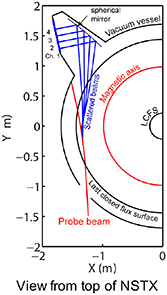
Figure 2. View from the top of the high-k scattering diagnostic in NSTX for shot 141 767. Due to its tangential geometry and close to midplane propagation, this diagnostic was initially designed to detect fluctuations with high kr and small  . We will see how fluctuations have smaller kr than previously expected, due to non-intuitive geometric effects in realistic flux-surface geometry, making the high-k scattering system more transport relevant than previously expected.
Download figure:
Standard image High-resolution image4.2. Nonlinear gyrokinetic simulation set-up
In our attempt to establish quantitative comparisons of electron-scale turbulence we present two types of non-linear gyrokinetic simulations: standard electron-scale gyrokinetic simulation featuring a box size characteristic for the resolution of electron-scale modes  and 'big-box' electron-scale simulation with an increased simulation domain
  . The increased simulation domain results in a finer wavenumber grid resolution, which proves necessary to resolve the experimental wavenumbers from the high-k system.
4.2.1. Physics parameters and numerical resolution
The physics parameters employed in both simulation types are taken from NSTX H-mode plasma shot 141 767. Standard electron-scale and 'big-box' electron-scale simulations model three gyrokinetic species ( ). Simulations are performed in the local, flux-tube limit at the scattering location r/a ∼ 0.7, including electron collisions (νei ∼ 1 cs/a, but not ion collisions), background flow and flow shear (M ∼ 0.2− .3, γE ∼ 0.1−0.2 c
 cs/a) and fully electromagnetic fluctuations
  . Linear background profiles were simulated employing non-periodic boundary conditions in the radial direction with typical buffer widths
  , respectively, for standard electron-scale and 'big-box' electron-scale simulation. Parallel resolution employed 14 poloidal grid points (× 2 signs of parallel velocity), 12 energies and 12 pitch-angles (6 passing + 6 trapped). This choice of numerical grids was made according to previous convergence and accuracy tests for the GYRO code simulating microinstabilities in the core of NSTX [40] and was also tested for convergence for the present conditions [7].
4.2.2. Radial and poloidal wavenumber resolution
The radial and poloidal wavenumber resolution of the non-linear simulations is of crucial importance in order to accurately resolve the measured wavenumbers by the high-k system. Standard electron-scale simulation resolves only electron-scale turbulence wavenumbers ![$k_r\rho_s \ \epsilon \ [1, 50]$](https://content.cld.iop.org/journals/0741-3335/62/7/075001/revision2/ppcfab82deieqn156.gif) and
and ![$k_\theta\rho_s \ \epsilon \ [1.5, 65]$](https://content.cld.iop.org/journals/0741-3335/62/7/075001/revision2/ppcfab82deieqn157.gif) . 'Big-box' electron-scale simulation resolves electron-scale turbulence, similarly as electron-scale simulation, but includes modes characteristic of low-k instabilities, typically
. 'Big-box' electron-scale simulation resolves electron-scale turbulence, similarly as electron-scale simulation, but includes modes characteristic of low-k instabilities, typically ![$k_r\rho_s \ \epsilon \ [0.3, 40]$](https://content.cld.iop.org/journals/0741-3335/62/7/075001/revision2/ppcfab82deieqn158.gif) and
and  65−
85] depending on the plasma condition. However 'big-box' electron-scale simulation does not correctly resolve the full spectrum of ion-scale turbulence (which would require a poloidal wavenumber grid spacing dkθs ∼ 0.05−0.1). In addition, simulations are only run for electron time scales (T ∼ 20−30 a/cs, when ions have not had time to reach a fully saturated state). Consequently, 'big-box' electron-scale simulation should not be considered as a multiscale simulation, such as the ones documented in [57–61] by Howard et al and Maeyama et al. All electron-scale simulations presented are converged in radial and poloidal box-sizes Lr and
65−
85] depending on the plasma condition. However 'big-box' electron-scale simulation does not correctly resolve the full spectrum of ion-scale turbulence (which would require a poloidal wavenumber grid spacing dkθs ∼ 0.05−0.1). In addition, simulations are only run for electron time scales (T ∼ 20−30 a/cs, when ions have not had time to reach a fully saturated state). Consequently, 'big-box' electron-scale simulation should not be considered as a multiscale simulation, such as the ones documented in [57–61] by Howard et al and Maeyama et al. All electron-scale simulations presented are converged in radial and poloidal box-sizes Lr and  , radial resolution dr, poloidal wavenumber resolution
  , as well as in simulation run-time T [7]. Additional numerical resolution details can be found in table 1.
Table 1. Numerical resolution parameters typical of a standard and a 'big-box' electron-scale simulation: dr is the radial resolution ( are, respectively, the ion and electron sound gyro radius using electron temperature Te),
 ![$L_r [\rho_s]$](https://content.cld.iop.org/journals/0741-3335/62/7/075001/revision2/ppcfab82deieqn138.gif) is the radial box size, nr is the number of radial modes, max
is the radial box size, nr is the number of radial modes, max is the maximum radial wavenumber resolved,
 ![$L_\theta[\rho_s]$](https://content.cld.iop.org/journals/0741-3335/62/7/075001/revision2/ppcfab82deieqn140.gif) is the poloidal box size, d
is the poloidal box size, d is the poloidal wavenumber resolution, max
 is the maximum poloidal wavenumber resolved, nn is the number of toroidal modes, T is the simulation run time, dt is the simulation time step. Both simulation models only resolve electron-scale modes.
| dr |  | nr | max |  | d | max | nn | T(a/cs) | dt(a/cs) | |
|---|---|---|---|---|---|---|---|---|---|---|
| std. e-scale | 2ρe | 4.5 | ≈ 200 | 50.5 | 4 | 1.5 | 65 | 42 | 30 |

|
| 'big-box' e-scale | 2.5ρe | 20 | ≈ 500 | 30 | 20.6 | 0.3 | 65 | ≈ 200 | 30 |  |
Table 2. Comparison between the measured wavenumber components via high-k scattering from channels 1, 2 and 3 in Cartesian coordinates  , and the corresponding values mapped to the field-aligned coordinate definitions
  in GYRO/CGYRO [49–51]. Equation (8) was used to perform the mapping.
| Cartesian | Field-aligned | |||
|---|---|---|---|---|
 |
 |  |  | |
| Ch 1 | –18.84 | –3.47 | –2.57 | –5.34 |
| Ch 2 | –14.87 | –2.82 | –2.05 | –4.21 |
| Ch 3 | –11.00 | –2.37 | –1.54 | –3.45 |
Figure 3 displays the radial and poloidal wavenumber simulation grid from a typical electron-scale simulation (left) and a 'big-box' electron-scale simulation (right), along with mapped wavenumbers detected by channels 1, 2 and 3 of the high-k scattering system. The black dots denote the dominant wavenumber detected by each diagnostic channel  , and the ellipses surrounding them are the wavenumber resolution, denoting the 1/e amplitude of the effective wavenumber filter (scattering matrix). Ideally, one would want to simulate several radial and poloidal wavenumbers inside each
  ellipse to accurately replicate the experimental fluctuation measurement. However, due to a coarse wavenumber grid spacing, standard electron-scale simulation can at most resolve one radial and two poloidal wavenumbers inside the effective measurement range delimited by the elliptical shape of the wavenumber filter. This poor resolution due to the diagnostic requirements and numerical resolution requirements will result in inaccurate synthetic frequency spectra computed from electron-scale simulation (figure 8). By decreasing the wavenumber grid spacing (dkr, d
 ), a 'big-box' electron-scale simulation can effectively filter a handful of poloidal wavenumbers inside the measurement range from each channel, yielding it adequate for attempting quantitative turbulence spectra comparisons. This results in computationally intensive simulations, typically running on 10−20 thousand parallel CPU cores taking ∼1−
2 M CPU hours to completion on leadership high-performance supercomputers such as NERSC's Edison.
), a 'big-box' electron-scale simulation can effectively filter a handful of poloidal wavenumbers inside the measurement range from each channel, yielding it adequate for attempting quantitative turbulence spectra comparisons. This results in computationally intensive simulations, typically running on 10−20 thousand parallel CPU cores taking ∼1−
2 M CPU hours to completion on leadership high-performance supercomputers such as NERSC's Edison.

Figure 3.  grid for a standard electron-scale simulation having a conventional simulation domain
  (left) and an electron-scale simulation with increased numerical domain
  (right) along with the measurement range of channels 1, 2 and 3 of the NSTX high-k scattering system [26]. The ellipses denote the 1/e amplitude of the wavenumber filters in k-space. (a) The electron-scale simulation with a standard simulation domain does not accurately resolve the measurement wavenumbers from the high-k diagnostic due to a coarse
  grid. (b) An electron-scale simulation with increased simulation domain is needed to accurately resolve the measurement wavenumbers from the high-k scattering diagnostic. Reproduced from [7]. © IOP Publishing Ltd. All rights reserved.
Download figure:
Standard image High-resolution image
Figure 4. (a) Radial wavenumber filter  corresponding to a measurement wavenumber component kr+ (Gaussian shape, equation (12)). (b) Poloidal wavenumber filter corresponding to a measurement wavenumber component
  . The
. The  components correspond to channel 1 of the high-k scattering system from NSTX H-mode plasma 141 767. The Gaussian shape of
  and
and  comes from the Gaussian shape of the scattering volume U (figure 6). In red are the filters using the numerical grids from a standard electron-scale simulation, and in blue from a 'big-box' electron-scale simulation. Notice the lack of resolution when using a standard electron simulation, and the improved resolution when using a 'big-box' simulation, due to the finer wavenumber grid resolution.
Download figure:
Standard image High-resolution imageTable 3. Values for the total scattered power Ptot [a.u.], spectral peak <ω>
[cs/a] and spectral width ![$\sigma_\omega\ [c_s/a]$](https://content.cld.iop.org/journals/0741-3335/62/7/075001/revision2/ppcfab82deieqn264.gif) corresponding to synthetic frequency spectra from figure 8. Similar values of the total power Ptot and spectral peak <ω>
are obtained between the two simulation models (standard versus 'big-box' electron-scale simulation). The spectral width
corresponding to synthetic frequency spectra from figure 8. Similar values of the total power Ptot and spectral peak <ω>
are obtained between the two simulation models (standard versus 'big-box' electron-scale simulation). The spectral width  is wider for 'big-box' electron-scale simulation, in closer agreement to the experimental value (section 4.5).
| Ptot [a.u.] | <ω> [cs/a] | ![$\sigma_\omega\ [c_{s}/a]$](https://content.cld.iop.org/journals/0741-3335/62/7/075001/revision2/ppcfab82deieqn266.gif) |
|
|---|---|---|---|
| Std. e- scale | 1.82 10−11 | −24.18 | 3.04 |
| 'Big-box' e- scale | 2.17 10−11 | −23.29 | 5.13 |
4.2.3. Measured wavenumbers
Ray-tracing provides the measured wavenumbers in the components  . These are mapped to
  in figure 3 by use of the full 3D mapping (equation (8)). Since the measurement is local and close to the outboard midplane (poloidal location
  ), in what follows we present alternative calculations of the wavenumber mapping using the 2D and outboard midplane approximation (equation (11)), as well as a 'naive' mapping (equivalent to unshifted, circular flux surface geometry). These are presented for channel 1, which is sensitive to
  m−1.
m−1.
The 2D and outboard midplane approximation requires computing the geometric factors  and the GYRO normalizing
  . We use the flux-surface geometry of NSTX H-mode plasma 141 767, and find
  , κ ≈ 2.11, q ≈ −3.79,
  and
and  cm. Note here how
  is ∼ 3× smaller than the experimental, local value of ρs∼0.7 cm (due to the normalizing field
  in GYRO, which does not correspond to the local value). Using the 2D and outboard midplane approximation (equation (11)) we find that the wavenumber components from channel 1 map to
  . For comparison, the full 3D mapping of equation (8) gives
  , which corresponds to the plotted values for channel 1 in figure 3. The kr component is very well reproduced, but an error of ≈ 20%−25% is produced in the
  component. This discrepancy emphasizes the importance of using the full mapping for realistic tokamak geometry, even for rather small off-midplane poloidal angles
  . This is partly due to the larger kx + component of the high-k scattering system and the high flux surface shaping of this spherical tokamak plasma (which make the
  term non-negligible in the second line of equation (8)). The result of the mapping applied to channels 1, 2 and 3 is given in table 2.
Using the local ρs value as in experimental measurements gives the normalized  components from channel 1
  . If one were to make the 'naive' mapping
  and ignore the different ρs definitions, a significant systematic error of factor of ∼5× would be performed in the interpreted kr, and ∼ 2× in the interpreted
  . As a result, we learn that the high-k scattering system is sensitive to fluctuations with a lower kr and larger
  than predicted by the 'naive' mapping, bringing it closer to the streamer peak of fluctuations (figure 6). This makes the NSTX high-k scattering system more transport relevant than previously thought, and emphasizes the importance of performing the wavenumber mapping (equation (8) or (11), depending on conditions) in order to correctly interpret the measurement range of the high-k diagnostic. As an illustration, figure 6 shows the mapped wavenumbers from channels 1, 2 and 3 using the full 3D mapping in black dots (equation (8)), and in white dots using the 'naive' mapping
  . These are superimposed on the 2D density fluctuation wavenumber spectrum
  .
.
4.2.4. Filters in wavenumber space and real space
For the same plasma discharge condition, figure 4 shows the shape of the radial and poloidal wavenumber filters  and
and  in the θ0 ≈ 0 approximation (equation (12)), using a simulation grid from a standard electron-scale simulation (red) and from a 'big-box' electron-scale simulation (blue). The Gaussian shape comes from the Gaussian shape of the scattering volume U (equations (6)). Notice the lack of resolution when using a standard simulation domain (red), particularly in kr, and the improved resolution when using a bigger simulation domain (blue), due to the finer
  grid resolution. The 'virtual' dashed line shows the theoretical Gaussian expression of the filter. Note we chose ΔZ = 3 cm (the experimental value) and ΔR = 1 cm (reduced from the experimental ΔR = 3 cm due to the reduced simulation domain, even for the increased box size). The reduced radial extent of the scattering volume ΔR in a local simulation only scales the fluctuation amplitude by a constant value of irrelevance in the current work.
Figure 5 shows a snapshot of the raw 2D electron density fluctuation field δn(R, Z, ϕ0 = 0) for a standard electron-scale simulation in 5(a) and for a 'big-box' electron-scale simulation in 5(b). The elongated streamer structures are tilted by the strong E × B shear flow. (c) and (d) show the corresponding electron density fluctuation field filtered by a 2D filter in real space  and selecting the
  wave-vector, respectively for a standard (c) and 'big-box' electron-scale simulation (d). Volume integration of
 ![$\textrm{Re}[\delta n(R, Z, \varphi_0 = 0)U(R-R_0, Z-Z_0)e^{-i \vec{k}_+\cdot \vec{r}}]$](https://content.cld.iop.org/journals/0741-3335/62/7/075001/revision2/ppcfab82deieqn214.gif) directly yields the synthetic signal of fluctuations
directly yields the synthetic signal of fluctuations  as in equation (3) (Re denotes the real part). Figures (c) and (d) give a spatial representation in real-space of the detected structures by the high-k system, and illustrate the effect of the filtering by U and wavenumber selection via the complex exponential
  . Since simulations are run in the local approximation, profile parameters are constant within the radial domain and the radial filter is chosen to be constant Ψr = 1. The poloidal filter shape is Gaussian in θ and mapped to (R, Z), having maximum amplitude at the thick black line passing through Z0 ≈ −0.06 cm. The additional black dashed lines denote the 1/e, 1/e2 and 1/e3 amplitude of the filter in the poloidal direction.

Figure 5. (a) and (b) 2D raw electron density fluctuation field δn mapped to cylindrical coordinates (R, Z, ϕ0 = 0), corresponding to an electron-scale simulation with standard domain  in (a), and increased simulation domain
  in (b). In (c) and (d) the 2D density fluctuation field δn has been multiplied by the 2D real space filter U(R – R0, Z – Z0) and by
  . The quantity
  – R0, Z –
 ![$Z_0)e^{-i\vec{k}_+\cdot\vec{r}} \big]$](https://content.cld.iop.org/journals/0741-3335/62/7/075001/revision2/ppcfab82deieqn210.gif) denotes the amplitude of the measured wavenumber
denotes the amplitude of the measured wavenumber  by the high-k system. The thick black line passing through Z0 ≈ −0.06 cm denotes the maximum filter amplitude poloidally, and the additional black dashed lines denote the 1/e, 1/e2 and 1/e3 filter amplitudes in the poloidal direction.
Download figure:
Standard image High-resolution image
Figure 6. 2D  spectrum of the electron density fluctuations normalized per radial and poloidal wavenumber step d
 and d
and d , corresponding to a standard electron-scale simulation in (a) and to a 'big-box' electron-scale simulation in (b). The improved resolution in k-space due to the increased box size makes a bigger domain more suitable for attempting quantitative comparisons between synthetic and experimental frequency spectra (section 4.5). Black dots and ellipses correspond to the measured wavenumber
  and k-resolution from three channels of the high-k diagnostic (the same as figure 3), computed using the full 3D mapping (equation (8)). White dots and ellipses are computed using the 'naive' mapping
  .
.
Download figure:
Standard image High-resolution image4.3. Electron-scale simulation spectra
In this subsection we show electron-scale simulation spectra to gain insight into the measurement range of the high-k diagnostic. Spectral differences between a standard electron-scale and a 'big-box' electron-scale simulation are also discussed.
Figure 6 shows the GYRO 2D electron density fluctuation power spectrum from a standard electron-scale simulation in (a) and a 'big-box' electron-scale simulation in (b), proportional to the spectral density  .
.  are the internal field-aligned definitions in GYRO. We define
  , where
  denotes the θ and time averages, and d
 , d
, d are the simulation radial and poloidal wavenumber grid resolutions. The black dots surrounded by ellipses correspond to the wavenumber measurement range from channels 1, 2 and 3 of the high-k diagnostic, the same as figure 3 shows. The spectrum is not symmetric in
  and is tilted due to the high E × B flow shear. The highest spectral power given by streamers is characterized by finite
  and
and  , consistent with the tilt of streamers in real space (figures 5(a) and (b)). Figure 6 is only intended to give a qualitative idea of the measurement wave numbers in the simulated fluctuation spectrum, since it is the amplitude δnnp that should be filtered in the scattering process (preserving phase information), but not the spectral density
  . This can be clearly seen from equations (2), (3) and (4).
Figure 7(a) and (b) shows the kr and  electron density fluctuation power spectrum S(kr) and
  from a standard electron-scale simulation (red) and from a 'big-box' electron-scale simulation (blue). We define
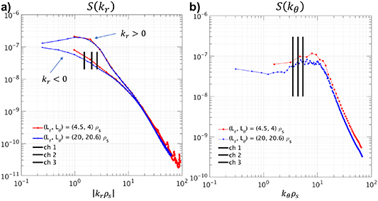
Figure 7. (a) Radial wavenumber spectrum of electron density fluctuations per radial wavenumber step d , computed by adding all
  contributions from
  . Since kr changes sign, the kr > 0 and
  branches are plotted. Adding only the
  contributions exalts the difference between measuring in the positive and negative kr part of the spectrum (the detected
  is
is  ). (b) Poloidal wavenumber spectrum of electron density fluctuations per poloidal wavenumber step d
 , computed by adding all kr contributions from
  (both kr > 0 and
  ). Due to the logarithmic scale and the symmetry property in δnnp,
  should be interpreted as having a negative sign
  . The measurement
  from channels 1, 2 and 3 are plotted as vertical lines in each figure.
Download figure:
Standard image High-resolution image
Figure 8. Synthetic frequency power spectrum of fluctuations  corresponding to a filtered wavenumber
  from channel 1 of the high-k scattering system. In red the synthetic spectrum corresponds to an electron-scale simulation, and in blue to a 'big-box' eletron-scale simulation. Two substantial differences are observed between both spectra. First, the standard electron-scale simulation exhibits a 'double-peak' structure that is not present in the 'big-box' electron-scale simulation. Second, the 'big-box' electron-scale simulation exhibits a wider spectrum, in closer agreement to experiment (section 4.5). The differences between both spectra are quantified in table 3.
Download figure:
Standard image High-resolution imageThe choice of  is made due to the symmetry property of the density spectrum
  (where * indicates the complex conjugate [49]). Vertical black lines indicate the measurement wavenumbers by the high-k system. Inspection of S(kr) in figure 7(a) emphasizes that the measurement is not aligned in kr with the highest amplitude streamer fluctuations (for
  , streamers have positive kr > 0 while the measurement is made for
  ). This suggests that it may have been possible to detect streamer fluctuations in the present experiment, had the measurement been designed for
  and kr > 0. Since kr changes sign, the kr > 0 and
  branches are plotted, exhibiting close to an order of magnitude difference in spectral power with respect to the streamer branch (kr > 0) near
  . The kr spectra between standard and 'big-box' electron-scale simulation exhibit quantitative agreement, from the low-k wavenumber peak of the spectrum to the spectral slope at higher kr.
Figure 7(b) shows the  density fluctuation power spectrum from a standard electron-scale simulation (red) and from a 'big-box' electron-scale simulation (blue). Due to the logarithmic scale and the symmetry property in δnnp (translating to
  ), the
  branch only is shown here and
  should be interpreted as having a negative sign (similarly to the negative kr branch in (a)). Figure 7(b) shows that the 'big-box' electron-scale simulation exhibits a quantitatively similar spectrum to a standard electron-scale simulation, showing similar wavenumber peaking and spectral slopes. However, the predicted spectral power is about ∼20% lower for the 'big-box' electron-scale simulation. This difference, however, lies within the simulation standard deviation of the total turbulent power. To summarize, figures 6 and 7 show how the 'big-box' electron-scale simulation spectra is quantitatively similar to that of a standard electron-scale simulation, providing ultimate confidence that the resolved electron temperature gradient (ETG) physics are very similar between the two simulation models.
4.4. Synthetic spectra and Doppler shift
In this section we deploy the 2D synthetic diagnostic for high-k scattering in k-space to show some of the spectral features of the synthetic spectra. The equivalence between the real space and the k-space implementation of the synthetic diagnostic is essentially identical, as shown in appendix C.
Figure 8 shows the spectral density  predicted from a standard electron-scale simulation (red) and 'big-box' electron-scale simulation (blue), exhibiting the same plasma physics parameters but different wavenumber grid-resolution. The synthetic spectra exhibit qualitatively similar features such as frequency response and power levels (within ∼20% agreement), which are quantified in table 3. However, the spectra exhibit at least two appreciable differences. First, the spectrum in red exhibits a 'double-peak' structure in frequency, whereas the blue spectrum shows only one hump. Second, the spectrum in blue is wider than the spectrum in red. The particular values of the total scattered power Ptot, the spectral peak <ω> and the spectral width
  are computed by analysis of the turbulence frequency spectrum
  in figure 8 (throughout this manuscript we denote 'spectral peak' as the frequency value <f > or <ω> at the peak of the spectral power). Table 3 shows the specific numeric values of Ptot, <ω> and
  .
.
As discussed in figures 3 and 4(b), the reduced wavenumber grid-resolution from a standard electron-scale simulation only allows it to sample a maximum of two simulation toroidal mode numbers contributing to the high-k signal. The two peaks in the red curve of figure 8 correspond to the two dominant toroidal mode numbers within the measurement  range. Each mode has its own propagation frequency and is additionally Doppler-shifted by a different amount (
 , where n+ is the sampled mode number and
  is the plasma toroidal rotation frequency). This results in a separation of spectral peaks in the frequency spectrum due to the two dominant modes contributing to the synthetic signal when using a small simulation domain (red spectrum). This phenomenon is not present when using an increased simulation domain (blue curve) due to the increased number of sampled modes. Using a bigger simulation domain increases the number of toroidal modes sampled within the measurement
  range, which tends to 'fill-in' the frequency spectrum and yield a single frequency feature in figure 8. This last point also contributes to a widening of the spectrum from a value of
  (red) to a value of ~ 5a/cs (blue, table 3), yielding an improved agreement with the experimentally detected spectra (section 4.5).
In the present conditions, the toroidal rotation level (Mach number M ∼ 0.2) added to the relatively high poloidal wavenumbers sampled ( –5) contribute to a Doppler shift frequency ωDop that can exceed the plasma-frame frequency of fluctuations by factors of ∼10× or more (recall
  ). The frequency spectrum of the high-k system is dominated by Doppler shift. To illustrate this, figure 9 shows the frequency power spectrum from a 'big-box' electron-scale simulation in which no Doppler-shift was applied to the fluctuations (gray), and with the experimental Doppler shift value applied (blue). The different frequency response between the two spectra highlights the important effect of Doppler shift in these conditions, shifting the peak of spectral power from
  with no Doppler shift applied (ω > 0 is in the electron diamagnetic drift direction) to
  when Doppler shift is applied (Doppler shift shifts the frequency spectrum to the ion diamagnetic drift direction). Other frequency spectra quantities such as the total power Ptot and spectral width
  are quantitatively similar (table 4). A difference of ∼30% can be observed in the total spectral power Ptot, which might be related to numerical errors, but also to a pure effect of Doppler shift.
Table 4. Values for the total scattered power Ptot [a.u.], spectral peak <ω> [cs/a] and spectral width ![$\sigma_\omega [c_s/a]$](https://content.cld.iop.org/journals/0741-3335/62/7/075001/revision2/ppcfab82deieqn279.gif) corresponding to synthetic frequency spectra from figure 9, showing the impact of Doppler shift on the frequency spectrum (M is the Mach number). Similar values of the total power Ptot and spectral peak
corresponding to synthetic frequency spectra from figure 9, showing the impact of Doppler shift on the frequency spectrum (M is the Mach number). Similar values of the total power Ptot and spectral peak  are obtained between the two simulation models, but the spectral peak is completely different: fluctuations propagate in the electron diamagnetic direction in the plasma frame (ω > 0 for GYRO), but are shifted strongly towards the ion diamagnetic drift direction by Doppler shift.
| Ptot [a.u.] | <ω> [cs/a] | ![$\sigma_\omega\ [c_{s}/a]$](https://content.cld.iop.org/journals/0741-3335/62/7/075001/revision2/ppcfab82deieqn281.gif) | |
|---|---|---|---|
| Plasma frame: M = 0 | 1.62 10−11 | 1.54 | 4.89 |
Lab frame:  |
2.17 10−11 | −23.29 | 5.13 |

Figure 9. Synthetic frequency power spectrum of fluctuations  corresponding to a filtered wavenumber
  from channel 1, using 'big-box' electron-scale simulation. The gray line shows the frequency spectrum in the plasma-frame, to which no Doppler shift has been added. The blue line shows the frequency spectrum in the lab-frame, to which the experimental value of Doppler shift has been added. The Doppler shift frequency is at least 10× the plasma-frame frequency of fluctuations and completely dominates the frequency spectrum. The difference between the two spectra is quantified in table 4.
Download figure:
Standard image High-resolution imageOne can gain further insight into the effect of Doppler shift by studying the 2D frequency spectra plots  and (ω, kr). Figures 10(a) and (b) show the synthetic frequency power spectrum of fluctuations
  computed from a 'big-box' electron-scale simulation, where spectra have been filtered in kr around the radial component kr + (from channel 1), but not in
  . The black vertical band shows the measurement range in
  . No Doppler shift is applied in (a), and the experimental Doppler shift value is applied in (b). Figures 10(a) and (b) show that the effect of Doppler shift is primarily a shift in frequency ω proportional to
  as expected. A smaller effect is a widening of the spectrum
  , which is negligible for the present conditions but becomes more important for higher toroidal rotation values and higher
  . The spectrum also shows how the positive
  part of the spectrum exhibits higher spectral power than the negative
  counterpart, consistent with the spectrum shape from figures 6 and 7.

Figure 10. Synthetic frequency power spectrum of fluctuations corresponding to channel 1 of the high-k system.  in (a)–(b) and
  in (c)–(d) are computed from a 'big-box' electron-scale simulation. The spectra in (a) and (b) have been filtered in kr around the radial component kr + . No Doppler shift is applied in (a) and the experimental Doppler shift value is applied in (b). The
  plots show that the impact of Doppler shift for different
  is primarily a shift in frequency ω for the different
  , namely
  as expected. The black vertical band shows the measurement range in
  . In (c) and (d) the spectra
  have been filtered in
  around the poloidal component
  . Differently to the
  spectra, the (ω, kr)-spectra show that Doppler shift essentially produces a similar frequency shift for all kr, also as expected for the present conditions. The black vertical band in (c) and (d) shows the measurement range in kr, while the white dashed line denotes the kr = 0 line.
Download figure:
Standard image High-resolution imageFigures 10(c) and (d) show the synthetic frequency power spectrum of fluctuations  computed from a 'big-box' electron-scale simulation, where spectra have been filtered in
  around the poloidal component
  (channel 1), but not in kr. The black vertical band shows the measurement range in kr and the white dashed line denotes the kr = 0 line. Differently to the
  spectra, the (ω, kr)-spectra show that Doppler shift essentially produces a similar frequency shift for all kr (corresponding to the same
  since it has been previously filtered in
  ), as expected for the current conditions (this may not be the case in far off-midplane scattering locations). As observed for the corresponding
  plots, one can notice the asymmetry in
  for positive versus negative kr: a higher spectral power is observed for positive kr > 0 fluctuations (to the right of the vertical white dashed line). This is once more consistent with the
  spectra from figures 6 and 7.
4.5. Comparisons with high-k scattering fluctuation measurements from NSTX
In this subsection we compare synthetically generated frequency and wavenumber spectra with experimentally detected high-k spectra. The present experimental conditions correspond to a highly unstable ETG regime from NSTX H-mode plasma discharge 141 767, which has been extensively analyzed in [7, 52, 53]. In this regime, ETG was shown to be the only microturbulence process able to predict experimentally relevant levels of electron heat flux, and ion-scale turbulence was shown to be fully suppressed by strong E × B shear flow.
Synthetic spectra are obtained from two GYRO 'big-box' electron-scale simulations (details in appendix A). The first one uses the nominal experimental profile values as input (blue), and predicts ∼30% of the experimental electron heat flux value. In the second one (red), the values of the normalized electron density gradient a/Lne, safety factor q and magnetic shear  are scaled from the experimental values in a sensitivity scan to maximize the ETG drive, which was able to reproduce the experimental electron heat flux value within uncertainty. The values are: a/Lne = 0.502 4 is the ETG stabilizing mechanism, scaled by 1σ experimental uncertainty, q = 3.410 3 (−10%) and
  (+20%). The uncertainty σ(a/Lne) was computed from uncertainty in the background electron density profile followed by a Monte Carlo analysis approach. More details on this discharge condition and the corresponding turbulent transport fluxes can be found in appendix A and [7].
Figures 11(a), (b) and (c) show the frequency power spectrum of the high-k scattering system from channels 1, 2 and 3, respectively, plotted in real frequencies f (MHz). In black are the experimental frequency spectra, and in blue the corresponding synthetic spectra from a 'big-box' electron-scale simulation using nominal inputs. Two main differences can be observed: (i) experimental spectra exhibit a high spectral peak at zero frequency, corresponding to spurious reflections of the input microwave beam in the plasma; and (ii) experiment exhibits an increased background noise level with respect to simulation. In fact, experimental spectra are affected by electronic noise as well as by additional electromagnetic emission from the plasma that does not directly correspond to a scattering process. For these reasons, experiment and simulation comparisons are done in a prescribed frequency band, delimited by the black vertical dashed lines in figure 11. Experimental spectra are not absolutely calibrated, and are consequently rescaled by a constant. The particular value of the scaling constant is chosen in order to minimize the total integrated power from the different channels with respect to the synthetic frequency spectra (a least-squares minimization of the power difference). All channels are scaled by the same constant, preserving the fluctuation level ratio and the k-spectrum shape.

Figure 11. Frequency spectra comparisons between high-k diagnostic measurements (black) and synthetic diagnostic (blue) from channels 1, 2 and 3. Synthetic spectra show the spectral density S(f) in log10 scale, and were generated using 'big-box' electron-scale simulation with the nominal profile values as input. Experimental and synthetic data are analyzed in a prescribed frequency band (dashed lines) to avoid the f = 0 spectral peak present in experiment and capture most of the turbulence power at  . Experimental spectra are not absolutely calibrated, and are rescaled by a constant to minimize differences in the total spectral power with respect to the synthetic spectra (least-squares minimization). All channels are scaled by the same constant, preserving the fluctuation level ratio.
Download figure:
Standard image High-resolution imageQualitatively, experimental and synthetic spectra in figure 11 exhibit similar frequency response. The spectral peak <f> shows quite good agreement with experiment, lying within ∼10% for all channels. The spectral width σf lies within ∼25% of the experimental value (for channel 3, the reduced Doppler shift from the experimental spectrum with respect to the f = 0 peak does not allow a reliable measure of the spectral width σf). Table 5 shows the particular values of <f > and width σf (kHz). With respect to the spectral power, channels 1 and 2 in figure 11 exhibit reasonable agreement, however, the synthetic power level from channel 3 overpredicts the experimental power level by over an order of magnitude. The disagreement in the spectral power is also clearly seen in the wavenumber spectrum of fluctuations in figure 13, and suggests this simulation is likely missing some necessary physics ingredient that is able to reproduce the shape of the wavenumber spectrum.
Table 5. Summary of the main frequency spectrum characteristics corresponding to figures 11 and 12. The spectral peak <f> and the spectral width σf (kHz) from the different channels are compared, corresponding to experiment and simulation. Two simulations are used, one using the nominal experimental profile values as input, and also a simulation using scaled gradients (within 1σ(∇ne), −10% q and  ). dP denotes a validation metric of distance between experiment and simulation total fluctuation power Ptot, as suggested by [62, 63]. The σf = 196 (kHz) value from channel 3 is given in parentheses due to the unreliability of measurement from the reduced Doppler shift (figures 11 and 12).
| dP | ch 1 | ch 2 | ch 3 | ||||
|---|---|---|---|---|---|---|---|
| /(kHz) | <f > | σf | <f > | σf | <f > | σf | |
| Exp. | — | –895 | 214 | –810 | 199 | –613 | (196) |
| Sim. (nominal) | 5.08 | –843 | 186 | –735 | 157 | –664 | 127 |
| Sim. (scan) | 1.53 | –878 | 196 | –746 | 147 | –672 | 126 |
Figure 12 shows similar experiment and synthetic frequency spectra comparisons, where the synthetic spectrum this time is computed from a simulation with scanned inputs in a/Lne, safety factor q and magnetic shear  , chosen to maximize the ETG drive. A different scaling constant than in figure 11 is applied to the experimental frequency spectra in order to minimize the difference spectral power between experiment and simulation (however, all channels are scaled by the same constant). A similar agreement within ∼10% and ∼25% is observed in the spectral peak <f> and width σf, respectively (table 5). Recalling that <f > is completely dominated by Doppler shift, agreement in <f> does not imply agreement with the intrinsic frequency of fluctuations in the plasma frame. With respect to σf, as shown in table 4, σf appears to be insensitive to Doppler shift in the present conditions. This means that the measured spectral width is essentially the same as the intrinsic plasma frame value, which is reproduced by the synthetic spectra within 25% agreement. Interestingly, the spectral peak and width from both simulations exhibit very similar values, suggesting the frequency spectra characteristics are insensitive to the turbulence drive.

Figure 12. The same as figure 11, but in this case the synthetic spectra (red) are computed from a 'big-box' electron-scale simulation with scanned drive terms input in GYRO: the electron density gradient a/Lne was scanned by 1σ uncertainty, safety factor q by –10% and magnetic shear  by +20%. Here as well the spectral density S(f) is displayed in log10, and is rescaled by a constant that minimizes the squared distance in total power, preserving the fluctuation level ratio between the channels.
Download figure:
Standard image High-resolution imageFigure 13 shows the wavenumber spectrum comparisons between experiment and simulation using the nominal experimental parameters (blue, corresponding to figure 11) and using the scanned input values (red, corresponding to figure 12). The wavenumber spectrum is calculated from the frequency spectrum by integration of the frequency spectra within the prescribed frequency band for each of the three available channels. In figure 13 only, it is the synthetic spectra that are scaled by a constant, not the experimental spectra. A different normalization constant minimizing the distance with respect to experimental spectra is applied to the blue and red synthetic spectra to yield a comparison of the shape of the wavenumber spectrum, but not the total fluctuation power.
Simulation using scaled gradients displays improved agreement in the shape of the k-spectrum. This can be quantified via a validation metric  between experiment and simulation. We define the validation distance
  of the total fluctuation power Ptot as a metric
  , as suggested in [62, 63]. Here the sum ∑i is over the different channels (i = {1, 2, 3}),
  and
and  are the total fluctuation power from experiment and simulation, respectively, and Δ indicates the standard deviation of the time series used to compute Pi. In the definition of
  ,
,  has been scaled by a constant in order to minimize the difference with respect to the experimental spectrum.
  is thus the minimum distance between experiment and simulation, where the minimization is carried out by the scaling constant (recall all channels are scaled by the same constant).
Using this metric, we find a value of dP = 5.08 for the simulation spectra using the experimental profile values. The simulation using scaled inputs yields an improved distance of dP = 1.53. For reference, a value of  is roughly equivalent to a difference between experiment and simulation of 7σ, while a value of
  roughly equates to a difference of 2σ. This substantial improvement in the shape of the wavenumber spectrum shows the strong sensitivity of the k-spectra to input parameters, and highlights how reasonable agreement in the shape of the spectrum can be obtained within small variations in the simulation input drive terms (
 ). Reference [7] contains additional information about these and additional simulations performed for this NSTX discharge.

Figure 13. Wavenumber spectrum shape comparisons between high-k diagnostic measurements (black) and synthetically generated spectra from 'big-box' electron-scale simulation using nominal experimental profiles as input (blue) and scanned profile values of  (red). Wavenumber spectra in blue correspond to the frequency spectra in figure 11, and in red to figure 12. In this plot only, the synthetic spectra are scaled by a different constant minimizing the distance with respect to experimental spectra, yielding a comparison of the shape of the wavenumber spectrum. Simulation with scanned profile values shows improved agreement in the shape of the k-spectrum with respect to experiment (quantified in table 5).
Download figure:
Standard image High-resolution image5. Discussion and conclusions
We have presented a formulation of two synthetic diagnostics for coherent scattering of microwaves and applied it to the particular case of the high-k scattering diagnostic in NSTX [26]. This has yielded direct comparisons between experiment and simulation of high-k frequency and wavenumber turbulence spectra. The principles outlined in sections 2 and 3 remain quite general and applicable to additional fluctuation diagnostics such as DBS, reflectometry, and even cross-polarization scattering (CPS) measurements. Although we have formulated a full 3D synthetic diagnostic in sections 2 and 3, we have only deployed a 2D synthetic diagnostic in section 4. Appendix E includes additional insight on the differences expected in a 3D formulation.
This work has built on previous synthetic diagnostic efforts of high-k scattering [42] and DBS [45], which were based on the standard interpretation of scattering in k-space. We have shown the equivalence of the formulation in k-space to a formulation in real space. Agreement between the two formulations is also achieved numerically in realistic flux-surface geometry (appendix C), providing improved confidence in the synthetic calculations presented. Additional insight into the measurement can be gained via the implementation in k-space, which provides precious information about the measurement wave-vector  mapped to the field aligned
  components. In particular, the k-space implementation shows that a 'big-box' electron-scale simulation is more suitable for attempting quantitative comparisons with experimental turbulence measurements, as figure 3 shows. A detailed understanding of purely numerical artifacts in the frequency spectra (figure 8) was only possible with the wavenumber formulation of the synthetic diagnostic. This information would not have been available if only the real space formulation was implemented. We highlight that full understanding of the specific scattering measurement and corresponding numerically generated synthetic spectra can only be gained with the combined implementations in real space and in k-space.
Part of this work has shown how the measurement wavenumbers from the high-k scattering system are much closer to the peak of the fluctuation spectrum (streamers) than was previously thought. The mapping between cylindrical and field-aligned wavenumber components (equation (8)) has highlighted three main geometric effects affecting the interpretation of the measured wavenumber: the effect of the normalizing magnetic field entering the definition of ρs, the effect of Shafranov shift Δ affecting the radial wavenumber component kr through compression of flux surfaces at the outboard midplane, and the effect of flux-surface elongation κ affecting the poloidal wavenumber  through flux surface stretching poloidally. These three effects combine to yield systematic errors in the interpretation of the measured wavenumber components of up to factors of 5 in the present conditions. These systematic errors are amplified in conditions of strong Shafranov shift and highly shaped geometries in spherical tokamaks.
We find that the high-k scattering system in NSTX is sensitive to –3, 3–6) . Although the high-k scattering system was initially designed to be sensitive to high-kr and low- fluctuations, we find that the corresponding
  values are not as high-kr as originally thought (as predicted by the 'naive' mapping), while the
  component is higher (the high-k diagnostic is sensitive to high-kx in the lab frame, but this does not necessarily map to high-kr in the field-line frame). The smaller
  and larger
  values with respect to a 'naive' mapping indicate the measurement k by the high-k scattering system is more transport relevant than previously thought. Figure 6 shows how close the high-k measurement is to the streamer peak of the fluctuation spectrum. This hints at the possibility that the high-k scattering system may in fact already have been sensitive to streamer fluctuations for other experimental conditions and high-k scattering geometry. A careful analysis of additional NSTX plasma discharges to the one presented here would be needed in order to confirm this speculation. Additionally, a newly designed high-k scattering diagnostic is planned to be installed in NSTX-U. Projected to be sensitive to smaller kr and higher
  , it is also expected that this diagnostic will be able to detect density fluctuations from streamers.
This work has highlighted the profound impact of Doppler shift on the measured high-k signal, making the frequency spectrum of fluctuations completely dominated by Doppler shift. In particular, figure 9 and table 4 show how the spectral peak of fluctuations shifts from a value of < ω> ∼ 1.5 cs/a in the plasma frame, to a value of ∼−23 cs/a in the lab frame. This suggests the spectral peak of the high-k measurement is completely opaque to the intrinsic plasma frame value, making it nearly useless as a quantitative discriminator on the turbulence model. In fact we have observed very close agreement in the spectral peak for the different turbulence models tested (standard electron-scale simulation, 'big-box' electron-scale simulation, simulations with scaled inputs, etc), as long as a correct Doppler shift value is applied. This can also be observed from tables 3 and 5.
With respect to the spectral width  , it is shown to be less affected by Doppler shift for the present case, however, one should be careful to interpret the measured width as an intrinsic turbulence value. As we have seen in figure 8 and table 3, a simulation with an increased simulation domain can modify the predicted spectral width from a value of
  to a value of ∼5 cs/a, for the same simulation physics parameters. Even with this improvement, a 'big-box' electron-scale simulation tends to underpredict the measured spectral width of fluctuations by ∼25% (figures 11, 12 and table 5). We interpret the improved agreement achieved by the 'big-box' electron-scale simulation to be due to the increased numerical resolution in k-space as suggested by figure 3. This also suggests that simulations having even higher wavenumber resolution and including additional physics, i.e. as multiscale simulation, could in fact provide a closer match to the measured spectral width of fluctuations.
This discussion aims to make the reader aware of the difficulty in interpreting the measurement frequency spectra characteristics from high-k scattering. Fortunately, we find that all the previous effects polluting the high-k frequency spectrum appear to have a less profound impact on the total fluctuation power Ptot, implemented in the wavenumber spectrum. Integration of the frequency spectrum along a prescribed frequency band seems to 'erase' artificial numerical artifacts present in the frequency spectrum. The relative fluctuation power also provides a precious constraint on the simulations through the characterization of the shape of the fluctuation wavenumber spectrum. This allows the possibility of model selection and discrimination, as we have seen from figure 13 and table 5 (even in the absence of absolute diagnostic calibration). Even though the comparisons between experiment and simulation presented remain at a preliminary stage, they beg for additional quantitative comparisons of turbulence wavenumber spectra in future high-k scattering experiments. Improved diagnostic capability (only three channels are available in this work) as well as absolute diagnostic calibration would provide highly valuable validation constraints.
There is no doubt that the synthetic high-k turbulence predictions presented here suffer from uncertainties and inaccuracies emanating from the approximations made in the synthetic model. One important approximation lies in the 2D implementation, which is discussed in appendices E and F. An additional approximation in the synthetic diagnostic described here is based on a constant k: the same turbulence wavenumber is sampled within the whole simulation domain. In fact, the measurement wavenumber provided by ray-tracing calculations is only representative of the central ray of the input microwave beam. However, in reality a slightly different wavenumber is sampled by the diagnostic at different radial, poloidal and toroidal locations within the scattering volume. To assess the impact of this constant-k approximation, additional ray-tracing calculations for non-central rays were carried out within the scattering volume, showing that the measured k can vary at most by ∼20%. This would have a small impact on the synthetic frequency and k-spectrum characteristics when compared to other factors such as the simulation wavenumber resolution or Doppler shift. However, it is possible that taking into account the spatial variation of  within the scattering volume could recover the underpredictions observed in the frequency spectral width in table 5 and figures 11 and 12. The spatial variation of
  could be computed through ray-tracing of non-central rays, beam-tracing, or even full-wave simulation, and is left for future work.
The work presented here is part of the broader framework of validation of turbulent transport models. The ultimate goal of the validation effort is to provide confidence that current models are able to explain the transport processes observed in present experiments, in order to be able to predict the plasma profiles and ultimately fusion performance of future fusion reactors. Although seemingly far from this ultimate goal, establishing quantitative turbulence comparisons via synthetic diagnostics is a necessary step for the validation of the fundamental first principles based simulations. From these, reduced models can be optimized and be subsequently used for profile prediction and performance prediction of future devices. Great strides have been made so far to predict the plasma density and temperature profiles of the spherical tokamak, but work is still in its early stage. This work serves as a stepping stone towards validating first principles based electron-scale simulation in the core-gradient region of modest-β NSTX NBI-heated H-modes. We have found with reasonable confidence that electron-scale simulation is in fact able to reproduce the detected frequency and wavenumber spectra by the high-k scattering system in a highly unstable ETG regime. Improved confidence in the current transport models will only be possible by placing additional constraints via additional diagnostic measurements and further testing of the models in higher-β, lower collisionality and higher performance plasmas. Combining high-k measurements to low-k and intermediate-k fluctuation diagnostics (DBS, reflectometry, BES), magnetic field fluctuation measurements (CPS), etc, would provide invaluable information to constrain our turbulence models at all relevant spatial and temporal scales characteristic of microturbulence fluctuations. More importantly, they are imperative to test and validate our current models in the wake of future fusion generating devices such as ITER and beyond.
Acknowledgment
The authors would like to thank all co-authors for fruitful discussions and invaluable advice. This work is supported by the US Department of Energy Contract DE-AC02-09CH11466, and partially by the Engineering and Physical Sciences Research Council (EPSRC) [EP/R034737/1]. Computer simulations were carried out at the National Energy Research Scientific Computing Center, supported by the Office of Science of the US DOE under Contract No. DE-AC02-05CH11231, and at the MIT-PSFC partition of the Engaging cluster at the MGHPCC facility (www.mghpcc.org), which was funded by DOE grant number DE-FG02-91-ER54109. The digital data for this paper can be found in http://arks.princeton.edu/ark:/88435/dsp018p58pg29j.
: Appendix A: Experimental plasma parameter input in GYRO
Table A1. The plasma parameter input in GYRO simulations presented in this work. Empty values in the last column 'Input value (scan)' simulation mean these values are identical to those in the column 'Input value (nominal)'.
| GYRO parameter | Input value (nominal) | Input value (scan) |
|---|---|---|
| r/a | 0.70 839 | |
| R0(r)/a | 1.522 7 | |
| Δ = dR0(r)/dr | –0.30 412 | |
| κ | 2.112 7 | |
 |
0.153 963 | |
| δ | 0.248 295 | |
 |
0.323 972 | |
| q | 3.789 2 | 3.410 3 |
 |
1.804 7 | 2.165 6 |
 |
0.00 328 | |
 |
0.16 | |
 |
0.125 8 | |
 |
1.036 2 | |
| νei | 1.379 113 | |
| Zeff | 1.950 4 | |
 |
0.78 503 | |
 |
0.035 828 | |
 |
1.135 2 | |
 |
1.135 2 | |
| a/LnD | 1.497 3 | |
| a/LnC | -0.876 9 | |
| a/Lne | 1.004 8 | 0.502 4 |
| a/LTD | 2.959 9 | |
| a/LTC | 2.959 9 | |
| a/LTe | 3.362 6 | |
| βe | 0.002 736 | |
| λD/a | 0.000 0 371 | |
 |
60 | |
 |
4.271 4 | |
| Te (keV) | 0.39 060 | |
| Bunit | 1.44 613 | |
| a (m) | 0.601 2 | |
 |
2.274 9 |
: Appendix B: Summary of the necessary scattering equations
We define here all the relevant quantities necessary to obtain the real-space and k-space computation of the synthetic signal  in section 2, from knowledge of the density perturbation
  and the filter in real space
  :
:
From the computation of the synthetic signal  , here is a summary of the formulas needed to achieve the final expression for the scattered power Ps as a function of the spectral density
: Appendix C: Equivalence between the real-space and k-space synthetic spectra computed by GYRO
In this appendix we compare the output of the synthetic spectra predicted from the real-space formulation versus the k-space formulation. Figure C1 shows the synthetic frequency power spectrum of fluctuations  corresponding to a filtered wavenumber
  from channel 1 of the high-k scattering system. Simulations use a big numerical domain
  . The formulation based on real-space (dashed line) is compared to the formulation based on k-space filtering (continuous line). Quantitative agreement is obtained between the two synthetic diagnostic formulations, achieving 15% agreement in the total power Ptot, and a further improved agreement in the spectral peak <ω> and spectral width
  . This agreement is not coincidental but is generally observed, and validates the implementation of both synthetic diagnostic methods in the context of realistic flux-surface geometries.
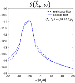
Figure C1. Synthetic frequency power spectrum of fluctuations  corresponding to a filtered wavenumber
  from channel 1 of the high-k scattering system. The synthetic spectra computed from the real-space implementation (dashed line) agrees with the synthetic spectra from the formulation based on k-space (continuous line), providing confidence on the validity of the computed synthetic spectra.
Download figure:
Standard image High-resolution image: Appendix D: Derivation of the wavenumber mapping to field-aligned coordinates
In this section we present a derivation of the wavenumber mapping to field-aligned geometry. The wavenumber components  mapped to field-aligned geometry allow for a direct interpretation of the measurement range of the high-k diagnostic. Figure D2 shows the reference geometry definitions in real space and in k-space that are used in this article.

Figure D2. (a) Cylindrical coordinates (R, Z, ϕ) used to express density fluctuations amplitudes  for deployment of the synthetic diagnostic in real space. (b) Definitions of wavenumber
  components in Cartesian coordinates
  . Due to axisymmetry the scattering location is assumed at ϕ0 = 0. The dashed vector corresponds to the projection of
  into the (X, Y) plane.
Download figure:
Standard image High-resolution imageIn real-space cylindrical coordinates (R, Z, ϕ), we define the wavenumber components  by
by
Since we assume axisymmetry, the reference frame is chosen at a fixed toroidal angle ϕ = 0 as figure D2 indicates. Associated to the field-aligned coordinates (r, θ, ϕ), the wavenumber components (kr,  ,
,  ) are internally defined in terms of n, p and
Recall the expansion of a generic fluctuating field in GYRO/CGYRO (ignoring Doppler shift) is  , and where α = ϕ + ν(r, θ) [49–51]. The radial wavenumber component kr is based on a Fourier decomposition of f in the radial coordinate (note
  ). The poloidal wavenumber
  is a flux surface quantity, independent of θ. The toroidal wavenumber
  has the same definition as in cylindrical coordinates, here
  . Note how
  , also consistent with figure D2(b). With these definitions, the wavenumber mapping from Cartesian coordinates
  to field-aligned coordinates
  is computed for a fixed toroidal mode number n and a fixed radial mode number p (recall equation (4)). Defining
  , we have
The last equality shows the definition of  . Note how
  since
since  only applies to the rapidly oscillating part of the fields. Making use of the chain rule yields
This relation being true for any arbitrary function znp, we arrive to the wavenumber mapping relations, relating a measured wavenumber  with components
  (in the form typically issued by ray-tracing codes or equivalent) to the field-aligned components
Equation (D8) is over constrained, and one needs to define two separate mapped toroidal mode numbers  and
and  , in addition to p+ (which are generally not integers). Using α = ϕ + ν(r, θ) we recover formula (8) used in the main text:
Using these relations, the wavenumber components  typically given by experiments can be mapped to the field-aligned wavenumber definitions
  employed by simulation codes using (D8), or equivalently to the mode number components
  using (D9). In equation (D9)
  denotes a toroidal mode number mapped from a vertical component kz + (not quite a poloidal component), while
  is a toroidal mode number mapped from a toroidal component ky + . These, in principle, need not be equal to each other. However, as we will see in the following appendices, the condition for successful scattering
  is equivalent to
  .
.
: Appendix E: Derivation of the scattering signal
In this appendix we show a more detailed derivation of the computation of the synthetic signal of density fluctuations  than the one presented in section 3. We start by rewriting the scattering signal in cylindrical coordinates (R, Z, ϕ), equation (3), repeated once more for reference:
where  is the measurement wavenumber in a particular scattering experiment, assuming constant in time and space in this work. The scattering volume shape U is centered around
  , and has the spatial extent ∼(ΔR, ΔZ, Δϕ). We place ourselves at the outboard midplane and assume Z0 ≈ 0. As in appendix D and in the main text, we choose a coordinate system in which the toroidal angle of scattering is set to ϕ0 = 0 (figure D2). The quantities ΔR, ΔZ, RΔϕ are much smaller than minor radius a but much greater than the corresponding wavelengths associated to
  .
.
The product  written in cylindrical coordinates is

Expanding the density field as  (ignore here Doppler shift
  ) and plugging into equation (E10), we recover equations (4) and (5):
We have assumed a slowly varying  in θ. At the outboard midplane it is reasonable to assume a scattering volume envelope to be separable in (R, Z, ϕ), such as
  , and assume these functions are well approximated by Gaussians (equation (6)). Now the scattering signal
  can be written as separate integrals over R, Z, and ϕ as
where we used expression (E11) for  . Since we assume a localized measurement in ϕ, the sin and cos terms in the exponent can be expanded about ϕ ≈ 0, leading to

Using this expansion, the integral  can then be written as
We assumed R ≈ R0 in Φn due to the slow spatial dependence on (r, θ), and we made use of the wavenumber mapping of equation (D9). The expression for Φn is nothing but a Gaussian integral, leading to
We recover a Gaussian shape for Φn. The toroidal mode number resolution  is complex in nature, and depends on the toroidal extent of the scattering volume Δϕ and the x component of the sampled wavenumber kx+. The combination
  is dependent on the specific scattering experiment and geometry and would have to be analyzed case by case. Now the scattering signal
  can be written as
The complex exponential part in  can also be expanded about
  , leading to
We can also expand (R, Z) about  in the expressions for
  (equation (6)), leading to
where  and Δθ = ΔZ/(r0κ). Next we can write the Jacobian Jr from
  approximately as
  . Putting equations (E16), (E17), (E18) and (E19) together, we arrive to the final expression of the scattering matrix Unp
Equation (E20) gives the general expression of the scattering matrix Unp in 3D and 2D, at the outboard midplane and assuming axisymmetry. The scattering signal can be computed similarly as before via  .
.
The different radial mode number filter Πp in a local versus global simulation stems from the fact that local simulation has the same profiles along the full radial domain. One can choose a radial filter in real space Ψr = 1, resulting in the sinc function. The toroidal, poloidal and radial mode number resolutions are
With respect to the toroidal filter, in the 2D approximation  , or equivalently
  , is a delta function, and the toroidal mode number filter Φn is simply constant. Taking into account the toroidal variation of the scattering volume leads to a combination of two toroidal mode number filters Φn and Θn. The toroidal filter in real space
  gives rise to a toroidal mode number filter Φn about
  . The poloidal filter in real space (ΨZ or
  ) gives rise to a toroidal mode number filter Θn about
  . However, recall how
  and
and  are a priori independent, since they are separately computed from
  and ky+, respectively. The question remains whether
  and
and  have similar values in actual scattering experiments. Assuming simple s−α geometry at the outboard midplane, equation (D9) simplifies to
Equation (E20) suggests the condition  is needed for achieving a finite amplitude scattering signal. Using equation (E22), the condition
  translates to the condition
  , i.e. fluctuations are aligned with
  . The condition
  is a necessary requirement for scattering experiments in magnetized plasmas, since fluctuations have maximal amplitude when aligned along the magnetic field. This information is directly encoded in the magnetic geometry along the field lines via the definition of ν and ultimately in the scattering matrix Unp. Successful, dedicated scattering experiments should be designed to satisfy the scattering condition
  , which is recovered here in the context of the computation of the scattering signal.
: Appendix F: Consequences of the 3D implementation for the high-k scattering system in NSTX
In this appendix we question whether toroidal effects are important for the high-k scattering system in NSTX. The scattering spectra presented in this article have been computed in the 2D approximation, i.e. setting  . In fact, the synthetic diagnostic signal is scaled by R0Δϕ. In this appendix we relax that restriction to understand if toroidal, 3D effects will have important consequences on the scattering signal.
As is suggested by equation (E20), the most important dependence on toroidal mode number n from the scattering matrix Unp comes from the filters Φn and Θn. We wish to understand how Φn and Θn compare to each other for different values of the toroidal scattering volume length R0Δϕ. This is an unknown quantity so far, although good estimates could be found following the procedures outlined in [54, 55]. The 2D approximation can be recovered for  .
.
Figure F3 summarizes the preliminary analysis performed to assess the effect of the toroidal scattering length R0Δϕ on the filters. These tests were performed for scattering wave-vector components corresponding to channel 1 of the scattering system and using realistic NSTX geometry from H-mode plasma 141 767. The vertical extent of the scattering volume is taken to be ΔZ = 0.03 m, consistent with the high-k scattering system.

Figure F3. (a) Shape of toroidal mode number filter  (absolute value) for different toroidal length values R0Δϕ of the scattering volume. (b) Comparison of toroidal mode number filters Φn and Θn. (c) Comparison of the total effect of a varying toroidal length of the scattering volume R0Δϕ on the total product toroidal mode number dependence of the scattering matrix Unp, given by the product
  .
.
Download figure:
Standard image High-resolution imageFigure F3(a) shows the toroidal mode number filter Φn for varying values of the toroidal scattering length R0Δϕ  [0.001−0.6] m. Small values of
  m correspond to highly toroidally localized measurements. The toroidal mode number resolution
  (equation (E21)) is dominated by the 4/Δϕ2 contribution, and decreases with increasing R0Δϕ from R0Δϕ = 0.001 m to R0Δϕ = 0.05 m. In this situation Φn is a real quantity. As the toroidal scattering length R0Δϕ further increases for
  m, we are in the opposite situation and
  is now a complex quantity. In this situation, an increasing toroidal scattering length for values larger than 0.05 m has the opposite effect of widening the resulting toroidal mode number width
  , increasing from R0Δϕ = 0.05 m to R0Δϕ = 0.6 m. Note how the narrowest width in this scan was found for a value of R0Δϕ = 0.05 m. We now wish to compare the extent of these filters Φn to the toroidal mode number filter Θn.
Figure F3(b) shows an actual comparison of the toroidal mode number filters Φn (black) and Θn (red), defined in equation (E20), and corresponding to the narrowest toroidal width found in (a) for R0Δϕ = 0.05 m. The toroidal mode number filter Φn is wider than the filter Θn, even in this 'worst-case' scenario in which  was narrowest. This suggests than one can assume Φn to be constant in the regime of variation of Θn. The overall product
  is in orange. Comparing
  (orange) and Θn (black), the main impact of Φn is simply a scaling factor. However, the overall width of the filter seems not to be much affected by the inclusion of Φn.
Figure F3(c) shows the overall product  for all the corresponding values R0Δϕ performed in (a). As can be seen, varying R0Δϕ has negligible impact on the overall toroidal mode number filter product
  . This can be understood from figures F3(a) and (b), since the filter Φn is wider than Θn for essentially all values of R0Δϕ. Compared to Θn, Φn is well approximated by a constant and results in an excellent approximation
  . This recovers the 2D formulation of the synthetic diagnostic.
Although only a qualitative assessment, we have not numerically implemented a 3D synthetic diagnostic and cannot compare actual frequency power spectra from 2D and 3D synthetic diagnostics. However, this preliminary assessment on the wavenumber filters suggests that the effect of the toroidal extent of the scattering volume is expected to be negligible for the high-k scattering system in NSTX, and the 2D approximation holds to a high degree of accuracy. A more detailed analysis comparing the actual frequency spectra from 2D and 3D synthetic diagnostics, as well as additional assessments to the one presented here for other coherent scattering experiments, might be the object of a future publication.
: Appendix G: Intuition behind the wavenumber mapping
In this appendix we expand on the consequences of having off-midplane scattering locations on the wavenumber mapping. We also present intuitive pictures behind the effect the normalizing magnetic field, Shafranov shift and elongation affecting the wavenumber mapping  .
.
Figure G4 shows an example mapping of equation (8), corresponding to a pair  m−1 when the mapping is computed at different poloidal locations along the flux surface, and neglecting the influence of the toroidal component (2D approximation). A circular scattering volume cross-section in U at a fixed toroidal slice gives rise to a circularly shaped filter in
  as shown in G4(a). This is characteristic of the high-k scattering diagnostic in NSTX [26]. Figure G4(b) shows how a circularly shaped filter in
  is mapped to an elliptical shape in
  , depending on the flux-surface location where scattering takes place. The ellipse is elongated, and becomes slanted for off-midplane locations. Even a small kz + = 1 m−1 value maps to finite
  , which can itself be positive or negative depending on the location of scattering along the flux surface. This means that the same measurement of
  at different poloidal locations will be sampling different turbulent wavenumbers when expressed in
  , which are the properly normalized wavenumber components characterizing microturbulence fluctuations. This will result into different scattering amplitudes at each poloidal location. The particular case of outboard midplane location is discussed in subsection 3.3. The flux-surface geometry is taken from NSTX H-mode plasma discharge 141 767.

Figure G4. (a) Circular wavenumber filter shape  corresponding to a circularly shaped scattering volume U in (R, Z), for a fixed toroidal slice ϕ0 = 0. The circles indicate the 1/e, 1/e2 and 1/e3 amplitude of the filter k-space filter W in
  (equation (2)). (b) Colored dots are mapped wavenumbers in
  corresponding to a measurement of
  m−1, while the ellipses surrounding each mapped wavenumber denote the 1/e amplitude of the scattering matrix Unp corresponding to the different poloidal locations along the flux surface. (c) Poloidal locations θ0 used to compute the mapped wavenumbers and 1/e filter amplitudes of (b). The yellow star corresponds to the experimental location of scattering analyzed in this article with poloidal angle
  . The flux-surface geometry is taken from NSTX H-mode plasma discharge 141 767.
Download figure:
Standard image High-resolution imageWithin the 2D approximation and at the outboard midplane (equation (11)), one can also easily build an intuitive picture behind the effect of the normalizing magnetic field, Shafranov shift and elongation on the wavenumber mapping. We recall the 2D approximation of the wavenumber mapping here once more
Experiments tend to use local values of the electron temperature Te and magnetic field B entering the normalizing ρs, while gyrokinetic codes tend to employ internal definitions. In expression (G23), the subscript  means the values of the mapped wavenumbers have been properly normalized by ρs, using Te and B consistent with the normalizations in gyrokinetic codes. In this work we used the GYRO
  normalizing magnetic field [50] in
  . Not using the same normalizing magnetic field in experiments as in gyrokinetic codes will lead to a systematic error in the interpreted measured wavenumber components
  by a scattering experiment.
Shafranov shift Δ primarily affects kr due to the compression of flux-surfaces at the outboard midplane through  (Δ is negative at the outboard midplane, but positive at the inboard midplane). For a given radial perturbation of wavelength
  at the outboard midplane given by experiment, the strong radial compression due to Shafranov shift will mean a larger λr in the field-line frame than in the absence of compression (where
  ). Note how the same perturbation of wavelength λx in the lab frame fits in the radial domain in the absence of Shafranov shift in figure G5(a), but not with strong Shafranov shift. This will translate to a smaller kr component with respect to the absence of compression, resulting in
  in equation (G23). The opposite will take place at the inboard midplane.

Figure G5. (a) Schematic poloidal cross section of two circular flux-surfaces in the absence of Shafranov shift (left) and in the presence of a strong Shafranov shift (right). Due to the compression of the flux surfaces at the outboard midplane, a measured wavelength λx in the laboratory frame is mapped to a larger radial wavelength λr measured in the frame of the magnetic field line. (b) Effect of elongation κ on the poloidal wavelength  in the frame of the magnetic field line. Due to the stretching of the flux surfaces at the outboard midplane, a measured wavelength λz in the laboratory frame is mapped to a smaller poloidal wavelength
  measured in the frame of the magnetic field line.
Download figure:
Standard image High-resolution image
With respect to elongation, it primarily affects  due to flux-surface 'stretching' poloidally. For a given vertical perturbation of wavelength
  given by experiment, a strongly elongated plasma will have a smaller
  in the field-line frame than in the absence of elongation (κ = 1). This will translate to larger
  component when compared to the absence of elongation, resulting in
  in equation (G23). Note how the same perturbation of wavelength λz in the lab frame has a smaller poloidal extent (smaller
  ) in the presence of elongation in figure G5(b) than in the absence of elongation. The factor
  in equation (G23) appears due to the definition of
  as a flux function, and not a local quantity in θ.