Mineralogical Prediction of Flotation Performance for a Sediment-Hosted Copper–Cobalt Sulphide Ore

Abstract

As part of a study investigating the influence of mineralogical variability in a sediment hosted copper–cobalt deposit in the Democratic Republic of Congo on flotation performance, the flotation of nine sulphide ore samples was investigated through laboratory batch kinetics tests and quantitative mineral analyses. Using a range of ore samples from the same deposit the influence of mineralogy on flotation performance was studied. Characterisation of the samples through QEMSCAN showed that bornite, chalcopyrite, chalcocite and carrollite are the main copper-bearing sulphide minerals while carrollite is the only cobalt-bearing mineral. Mineralogical characteristics were averaged per sample to allow for a quantitative correlation with flotation performance parameters. Equilibrium recoveries, rate constants and final grades of the samples were correlated to the feed mineralogy through Multiple Linear Regression (MLR). Target sulphide minerals content and particle size, magnesiochlorite content, carrollite liberation and association of the copper and cobalt minerals with magnesiochlorite and dolomite were used to predict flotation performance. Leave One Out Cross Validation (LOOCV) revealed that the final copper and cobalt grades are predicted with an R² of 0.80 and 0.93 and Root Mean Square Error of Cross Validation (RMSECV) of 4.41% and 1.34%. The recovery of cobalt and copper with time can be predicted with an R² of 0.94 for both and an overall test error of 4.70% and 5.14%. Overall, it was shown that quantitative understanding of changes in mineralogy allows for prediction of changes in flotation performance.

1. Introduction

Geometallurgy is a discipline that seeks to systematically integrate planning practices to maximize resource efficiency of future and existing mining operations, by combining geological, mineralogical, geotechnical and mineral processing information to create a spatial model for production planning and management [1,2]. From a strategic perspective, geometallurgy informs mine planning by combining insight into the natural distribution of relevant orebody characteristics with the spatial clustering of properties according to their metallurgical response [3,4]. Mineralogical understanding of the deposit allows for the development of mineralogical tools and methods for geometallurgy [5].The majority of the world cobalt output is produced as a by-product of copper sulphide ores from sediment-hosted deposits of the Democratic Republic of Congo (DRC). As there are few sites processing such ore types, limited studies into the processing of copper and cobalt sulphide minerals exist [6]. Within these deposits, carrollite (Cu₂CoS₄) is the main cobalt-bearing mineral in the sulphide ore and common copper sulphide minerals are bornite (Cu₅FeS₄), chalcopyrite (CuFeS₂) and chalcocite (Cu₂S). Flotation is one of the first steps in the concentration of the valuable sulphide minerals [6,7,8]. Xanthates are the most common collectors used to concentrate DRC ores with typical recoveries averaging around 85% for copper and 60% for cobalt, and concentrate grades consisting of up to 45% Cu and 4% Co [8]. A review of literature shows that no kinetics data has been published on the flotation behavior of carrollite [9,10,11]. For example, for a Zambian concentrator a xanthate collector had superior performance in terms of kinetics, recovery and grade compared to other thiol collectors, but no quantitative assessment of the rate constant and equilibrium recovery was done [9]. Sodium IsoPropyl Xanthate (SIPX), Potassium Amyl Xanthate (PAX) and a blend of those collectors were evaluated for copper and cobalt recovery. In that study the highest cobalt recovery was 83%, with a grade of 1.88% Co, was obtained using a blend of SIPX and PAX, at a ratio of 3:1 [10]. More recently, it was reported that when using a dithiophosphate collector, 90% of the copper sulphide minerals and 93% of carrollite could be recovered from mixed oxide sulphide ore at ambient pH in a laboratory batch flotation experiment. Final concentrate grades after the sulphide flotation stage were 12.2% Cu and 0.38% Co [11].

Flotation processes are typically optimized through changes of reagent dosage and flotation times, without a proper assessment as to whether the mineralogy of the feed has changed [12]. Understanding the influence of mineralogy on process performance is an inherent part of mine value chain optimization through geometallurgy. Regarding flotation, geometallurgical understanding is obtained by analyzing the differences in mineralogy prior to and after the flotation process, followed by linking that information to the kinetics rate constant and measured recovery [13]. By combining mineralogical data with flotation performance data, it is possible to derive a predictive model for process recovery based on the mineralogy of the feed material. There are a number of mathematical models that can be used to model the flotation kinetics, which are commonly based on a rate constant, equilibrium recovery and the changes in recovery over time [14]. There are several recent investigations that have used mineralogy as a tool for understanding the flotation response of copper bearing minerals [15,16,17]. For sulphide ore from the Kamoa copper project, sample mineralogy was considered for flowsheet development, which showed that a re-grind circuit would be beneficial for recovering the remaining sulphide minerals [15]. Principal Component Analysis was used to predict the recovery of copper sulphosalts based on differences in target mineralogy of the feed samples [16]. On an industrial scale, it has been shown that quantitative mineralogical data has been key in understanding historical recoveries and for predicting copper recovery at the Kansanshi flotation circuit [17]. This paper explores the complexity of modelling the flotation of copper–cobalt sulphide ore as a function of the feed mineralogy, which will be the only changing variable in the experiments. The relationship between quantitative mineralogy obtained using QEMSCAN and the rate constant, equilibrium recovery and final grade of the flotation process will be investigated.

2. Materials and Methods

2.1. Materials and Preparation

A range of quarter drill core samples were supplied by a copper–cobalt producer operating in the DRC. The drill core samples are known to originate from different locations within the sulphide zone of the ore body, with a varying mass from 0.8 to 4 kg. Nine samples were selected based on their spatial location, providing samples that represent the mineralogical variability present in the deposit. All samples were crushed down to −2 mm in order to homogenize the samples and were split into 500 g representative subsamples using a riffle splitter. These were then ground for 20 min at 60% solids in a 300 by 160 mm rod mill operating at 65 rpm. The grinding media consisted of six stainless steel rods of 290 by 23 mm, weighing 1 kg each. The grinding process occurred up to a maximum of fifteen minutes before the flotation experiment, in order to avoid sample oxidation.

2.2. Flotation Tests

2.2.1. Reagents

Methyl Isobutyl Carbinol (MIBC), provided by Acros Organics (Geel, Belgium), was used as frother in all the experiments. The bulk copper–cobalt collector Danafloat 245, supplied by Cheminova A/S (Harboøre, Denmark), was used as a sulphide collector. This collector mainly consists of sodium O,O-diisobutyl dithiophosphate and was the best performing collector for copper and cobalt sulphide minerals in a previous study [11].

2.2.2. Flotation Procedure

The mining operation from which the samples originate does not currently process sulphide ore and thus a basic flotation procedure was designed to evaluate the flotation performance. An overview of the timings used in the flotation procedure can be found in

Table 1. Flotation procedure for the experiments described in this study, including cumulative timing of separation, duration of conditioning and flotation stages and reagent dosages.

Phase	Stage	Cumulative Timing	Conditioning	Flotation	MIBC	DF245
		min	min	min	g/t	g/t
Rougher	1. Conditioning collector	0	3	-	-	30
	2. Conditioning frother	3	1	-	50	-
	3. Concentrate 1	4	-	0.5	-	-
	4. Concentrate 2	4.5	-	0.5	-	-
	5. Concentrate 3	5	-	1	-	-
	6. Concentrate 4	6	-	1	-	-
	7. Concentrate 5	7	-	2	-	-
	8. Concentrate 6	9	-	2	-	-
Scavenger	9. Conditioning collector	11	3	-	-	30
	10. Concentrate 7	14	-	1	-	-
	11. Concentrate 8	15	-	2	-	-

. For the collector a dosage of 30 g/t at a concentration of 1% was used and a dosage of 50 g/t for the frother. In each experiment, eight different concentrates were collected. For each collected concentrate the copper and cobalt content were measured, after which the concentrates were combined into one cumulative concentrate. The mineralogy of the samples was obtained by submitting the cumulative concentrate and final tailings for QEMSCAN analysis. Due to the low mass of the supplied core samples, it was not possible to perform replicate flotation tests. To obtain an indication of the experimental error, a duplicate test was done with a second 500 g subsample of the 4 kg sample (sample S3). This showed that for Cu, the experimental error was 3.56% for recovery and 0.70% for grade. For Co, the experimental error associated with recovery was 1.91% and 0.12% for grade. The system was floated at ambient pH, which was measured prior to the experiment taking place. This measured pH for the nine different samples can be found in Appendix A. Both rougher and scavenger flotation stages were operated under similar operational conditions, in a one-liter Denver D12 flotation cell with an agitation rate of 1200 rpm and an aeration rate of 7 L/min. The flotation experiment took place at 30% solids, complementing the water used during the grinding process with tap water. Additional tap water was added prior to the scavenger flotation taking place, ensuring a pulp density of under 30% solids.

2.2.3. Chemical Analysis

Portable X-Ray Fluorescence (pXRF) was used to analyze the copper and cobalt content of the individual flotation products using a Delta Premium Handheld XRF Analyser (Olympus, Southend-on-Sea, UK). A measurement on a SiO₂ standard was performed between each measurement to determine the presence of any impurities during the analysis. The pXRF was set to analyze each sample for 1.5 min in total, with 45 s for beam 1 to detect the presence of heavier elements and 45 s for beam 2, to detect lighter elements. To improve the overall accuracy of copper and cobalt content estimation, an external calibration was done with an S4 Pioneer lab-XRF (Bruker, Coventry, UK) using 25 standards, yielding an ${\mathrm{R}}^2$ of 0.98 with a Root Mean Square Error (RMSE) of 1.47% for copper and a ${\mathrm{R}}^2$ of 0.99 with a RMSE of 0.32% for cobalt. In addition the copper and cobalt content derived from the QEMSCAN analyses was used for reconciliation of the pXRF data [18], with an R² of 0.93 and RMSE of 5.10% for Cu and an R² of 0.94 and RMSE of 1.44% for Co.

2.2.4. Mineralogical Analysis

The quantitative mineralogical analysis was carried out using a QEMSCAN 4300 at Camborne School of Mines, University of Exeter, UK. This consists of a Zeiss EVO 50 Scanning Electron Microscope (SEM) platform and four light element Bruker silicon drift droplet (SDD) X-ray detectors [19,20]. Selected samples were mixed with pure graphite powder to minimize particle density settling effects and prepared into 30 mm diameter polished epoxy resin blocks and analyzed using the field scan or PMA mode to determine the mineral abundance and liberation of these samples. Standard settings were used following details outlined in literature [21], with the fields scan mode using a 10 micrometers scan resolution and the PMA mode using a 2 to 4 micrometers scan resolution matched to the particle size range. Data acquisition used iMeasure v4.2 software (Thermo Fisher Scientific, Eindhoven, The Netherlands) and data processing used iDiscover 4.2SR1 and 4.3 (Thermo Fisher Scientific, Eindhoven, The Netherlands). For data processing, the developed database from a previous study was used [11], after which the other mineral phases were checked and refined.

2.3. Flotation Kinetics Modelling

The mineralogy-based modelling of the flotation performance presented in this paper focuses on the rougher stage. For batch flotation processes, the change in mineral recovery and rate constant follow the n-order kinetics model, as obtained from flotation kinetics modelling review studies [14,22]:

$$\frac{dR}{dt}=k·{\left(R_{eq}-R\right)}^n$$

(1)

where k is the rate constant value of the element or mineral, R the recovery at a point in time and $R_{eq}$ the recovery reached at equilibrium. Four common solutions to this differential equation were evaluated in this study. All solutions define the recovery at time t and have two characteristic parameters: a rate constant, denoted $k_1$ to $k_4$ hereafter, and an equilibrium recovery $R_{eq}$. The first investigated model (model 1) is the first-order dynamic model for flotation [23]:

$$R\left(t\right)=R_{eq}\left(1-e^{-k_{1}t}\right)$$

(2)

The second considered model (model 2) is the first-order solution with a rectangular distribution model for the rate constant, also known as the Klimpel model [24]:

$$R\left(t\right)=R_{eq}\left[1-\frac{1}{k_{2}t}\left(1-e^{-k_{2}t}\right)\right]$$

(3)

The third evaluated model (model 3), is the second-order dynamic model for flotation, defined as [25]:

$$R\left(t\right)=\left(\frac{R_{eq}{}^2{k}_{3}t}{1+R_{eq}{k}_{3}t}\right)$$

(4)

Finally, the fourth model (model 4) considered is the second-order model with a rectangular distribution for the rate constant [24]:

$$R\left(t\right)=R_{eq}\left[1-\frac{1}{k_{4}t}\ln \left(1-e^{-k_{4}t}\right)\right]$$

(5)

2.4. Regression Analysis

2.4.1. Variable Selection

Input variables considered for performance prediction are the modal mineralogy, minerals particle size, liberation, association and pulp pH. The independent variables were normalized with respect to the variable range prior to regression analysis. The Pearson’s product moment correlation coefficient (${\rho }_{X,Y}$) was calculated between all the variables using the following equation:

$${\rho }_{X,Y}=\frac{cov\left(X,Y\right)}{{\sigma }_X{\sigma }_Y}$$

(6)

where X and Y represent two random variables, cov(X,Y) the covariance between the two random variables, and σ the standard deviation of the two identified variables. To initialize the regression workflow, the influence of variables with the highest correlation coefficient was evaluated.

2.4.2. Multiple Linear Regression

Multiple Linear Regression (MLR) is a technique that allows, for a given dataset composed of m samples, to fit a response to n independent variables (n $\le$ m) using the following equation [26]:

$$y={\beta }_0+{\beta }_1{x}_1+{\beta }_2{x}_2\dots +{\beta }_n{x}_n+e$$

(7)

where ${\beta }_i$ are the regression coefficients and e, a residual. It assumes that there is a linear relationship between the independent variables (x_i) and the response variable (y). MLR was performed using the software Origin Pro 2019b (OriginLab, Northampton, MA, USA) which, for each regression model, specifies the precision, significance and significance per independent variable using the Student t-test. Using the correlation matrix and backward selection, combinations of different variables were rejected or accepted based on the increase in model precision and parameter significance.

2.4.3. Cross Validation

To validate the MLR models, Leave One Out Cross Validation (LOOCV) was used. LOOCV is a method that can be used with any form of predictive modelling, with the advantages that the overall test error does not tend to be overestimated and that the results will be the same. LOOCV uses a single observation out of the dataset for validation and the n-1 remaining observations are used as training set. The Root Mean Square Error of Cross Validation (RMSECV) for the n observations is estimated using [26]:

$${\mathrm{RMSECV}}_{\left(n\right)}=\sqrt{\frac{1}{n}{{\displaystyle \sum }}_{i=1}^n{\left(y_i-{\widehat{y}}_i\right)}^2}, i=1,\dots , n$$

(8)

Here $y_{\mathrm{i}}$ is the observed value and ${\widehat{y}}_{\mathrm{i}}$ the value predicted by the model.

2.5. Methodology

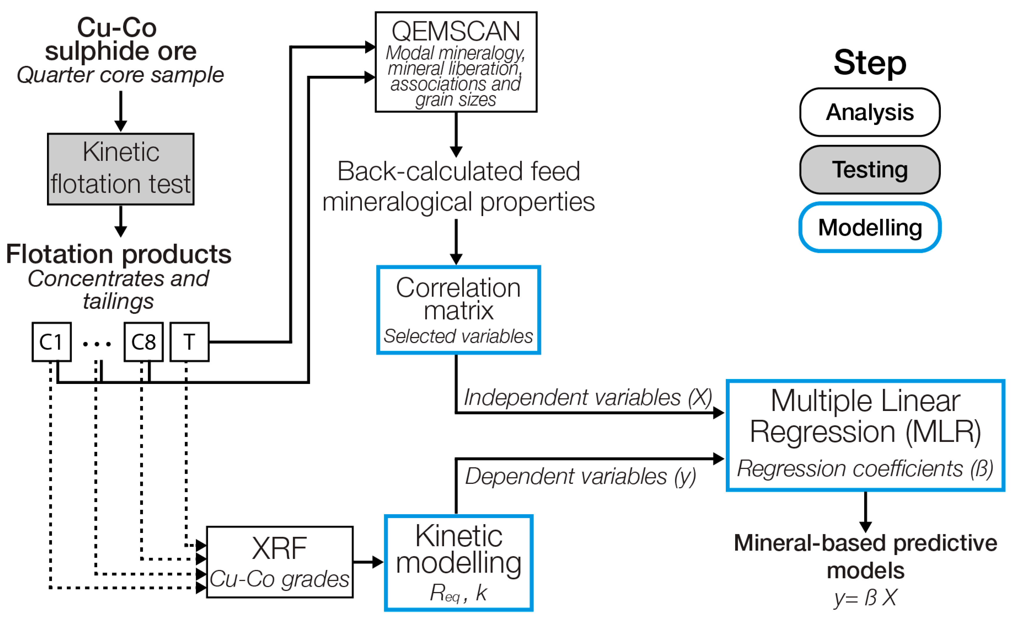
Using quantitative mineralogical data, regression analysis and cross validation, a model is developed that can be used to predict changes in copper and cobalt flotation performance based on in-deposit mineralogical variability. An overview of the methodology is shown in Figure 1. The work in this study can be classified in three categories. The experimental testing with standard operating conditions using nine core samples from different locations in the deposit (1), chemical analysis using pXRF and mineralogical analysis through QEMSCAN for each sample (2) and the modelling phase consisting of kinetics models fitting, using a correlation matrix for variable selection and MLR to quantify the impact of mineralogical parameters on flotation performance parameters (3).

3. Results and Discussion

3.1. Feed Characteristics

3.1.1. Feed Grade and Modal Mineralogy

The Cu and Co feed grade and the modal mineralogy of samples S1 to S9 are shown in

Table 2. Feed grade (pXRF) and modal mineralogy (QEMSCAN) of the nine different core sample sets (wt. %). Heterogenite, barite, gypsum, kaolinite, zircon and monazite were grouped as “others”.

Mineral/Element	Formula	S1	S2	S3	S4	S5	S6	S7	S8	S9
Carrollite	CuCo2S4	11.1	13.1	8.5	15.6	18.9	28.8	15.1	5.5	29.1
Chalcopyrite	CuFeS2	3.7	0.6	0.7	0.7	0.2	1.3	1.6	7.2	1.7
Bornite	Cu5FeS4	<0.1	14.7	32.6	27.3	11.1	41.6	31.1	0.1	6.4
Chalcocite	Cu2S	<0.1	0.8	0.5	0.8	5.7	4.4	1.5	<0.1	0.1
Pyrite	FeS2	1.0	0.1	0.1	0.3	0.1	0.2	0.3	<0.1	0.1
Chrysocolla	(Cu,Al)2H2Si2O5(OH)4·nH2O	0.3	0.2	0.1	0.2	0.1	0.3	0.6	0.3	0.2
Goethite	FeO(OH)	0.1	0.3	0.8	0.6	1.0	0.3	1.1	0.2	0.6
Rutile	TiO2	1.0	0.1	0.2	0.1	0.2	0.1	0.3	1.1	0.1
Dolomite/Ankerite	CaMg(CO3)2	2.5	44.6	16.7	18.1	44.9	10.7	12.9	12.1	27.3
Apatite	Ca5(PO4)3(F,Cl,OH)	0.4	0.3	0.6	0.2	0.3	0.2	0.7	0.6	0.4
Magnesite	MgCO3	<0.1	<0.1	2.0	0.1	0.2	0.1	0.6	<0.1	2.0
Quartz	SiO2	31.4	12.5	28.0	34.1	12.2	10.2	19.6	23.4	25.9
Plagioclase	(Ca,Na)(Al,Si)4O8	0.8	<0.1	<0.1	<0.1	0.1	<0.1	0.1	0.9	<0.1
K-feldspar	KAlSi3O8	31.1	<0.1	<0.1	<0.1	2.5	0.3	0.2	21.0	0.1
Muscovite/Illite	(Al,Mg,Fe)2(Si,Al)4O10[(OH)2,(H2O)]	10.0	<0.1	<0.1	<0.1	1.0	0.1	0.1	4.1	<0.1
Biotite	KFe3(AlSi3O10)(F,OH)2	2.4	<0.1	<0.1	<0.1	0.2	<0.1	<0.1	0.8	<0.1
Phlogopite	KMg3(AlSi3O10)(F,OH)2	2.0	<0.1	<0.1	<0.1	0.1	0.1	0.4	13.2	<0.1
Magnesiochlorite	(Fe,Mg,Al)6(Si,Al)4O10(OH)8	1.9	11.4	7.7	1.5	1.0	1.2	11.5	9.2	4.2
Mg silicates	Mg3Si4O10(OH)2	<0.1	1.1	1.3	0.3	0.2	0.1	2.0	0.1	1.6
Others		0.3	0.1	0.1	0.1	0.1	<0.1	0.1	0.1	0.1
Mineral Total		100	100	100	100	100	100	100	100	100
Cobalt	Co	1.5	3.1	1.6	3.7	6.5	8.6	4.2	1.4	6.3
Copper	Cu	2.1	7.8	14.3	13.1	11.5	18.2	15.7	2.5	6.4

. Overall, the samples are sulphide-rich, with a maximum of 76.3% (sample S6) and a minimum of 12.8% (sample S8) sulphide minerals in the feed. Carrollite is the only cobalt-bearing mineral. There are four different copper sulphide minerals, i.e., bornite, chalcopyrite, chalcocite and again carrollite. The content of these four sulphide minerals varies across the samples. Carrollite can be found in all the samples, whereas bornite, chalcocite and chalcopyrite in some cases are only present in trace amounts. The main gangue minerals present in all samples are quartz and dolomite. In some instances, K-feldspar and muscovite/illite are present in large quantities, for example in sample S1 and sample S8. Both the target sulphide minerals and the gangue minerals show considerable variation in these nine samples, indicating that the ore is heterogeneous throughout the deposit. In total, twenty-four minerals were detected, of which those present in trace quantities, notably heterogenite, barite, gypsum, kaolinite, zircon and monazite, were grouped as “others” in Table 2. A description of the minerals can be found in the Supplementary Material.

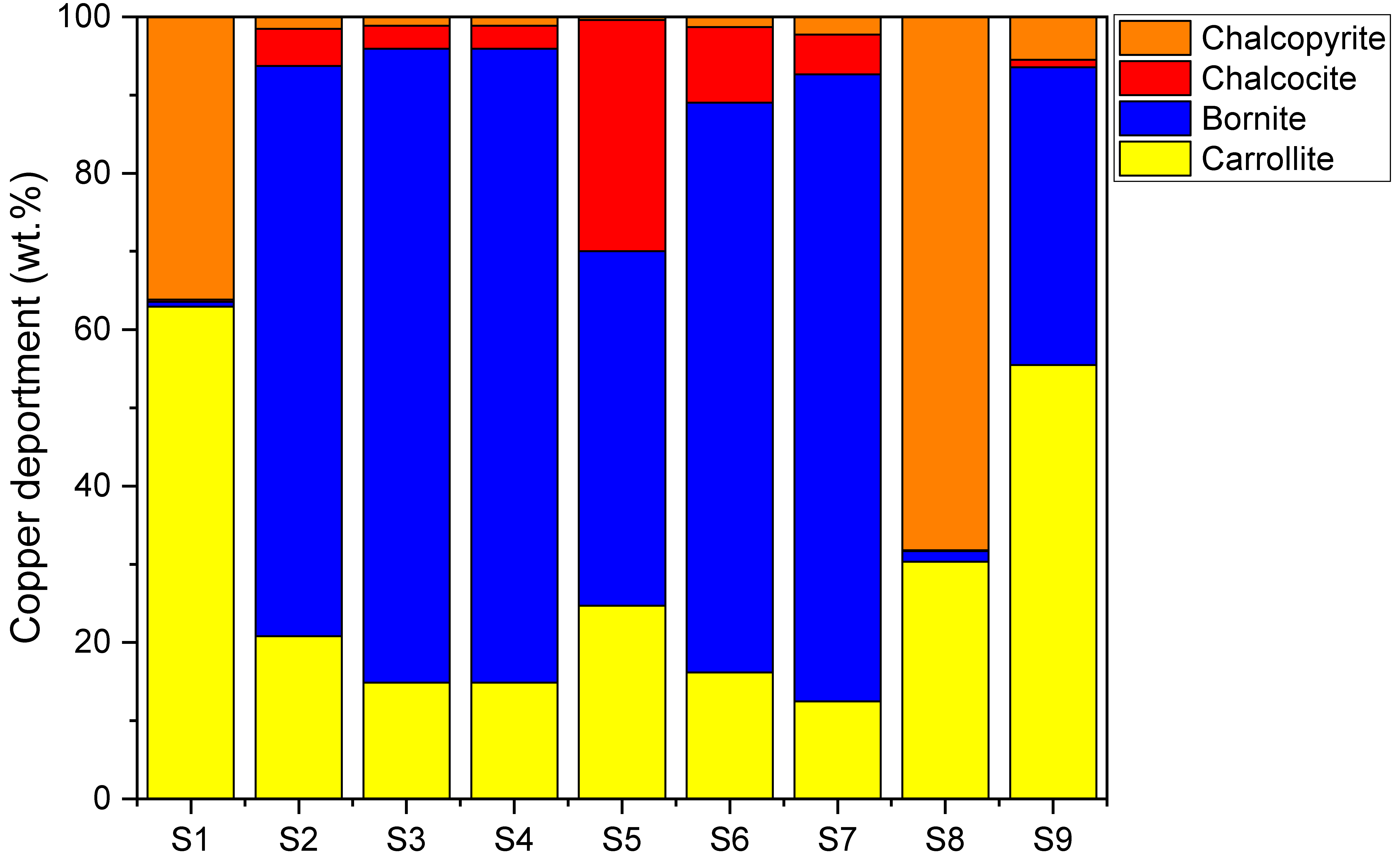
As carrollite is the only cobalt-containing mineral, cobalt recovery is directly related to the recovery of carrollite. For copper recovery, this type of relationship cannot be drawn. When considering Table 2, the quantity and ratio at which the four copper-bearing minerals are found in the samples varies. Using the mineralogical data from Table 2, the copper deportment in the different feed samples can be determined, as presented in Figure 2. For six out of the nine feed samples bornite is the main mineral contributing to the copper content. For sample S1 and S9, carrollite is the dominant mineral contributing to the copper content and for sample S8 that is chalcopyrite. Chalcocite is not the main copper carrying mineral in any of the samples. In sample S5 chalcocite contributes to around a quarter of the total copper content.

3.1.2. Feed Mineral Particle Size

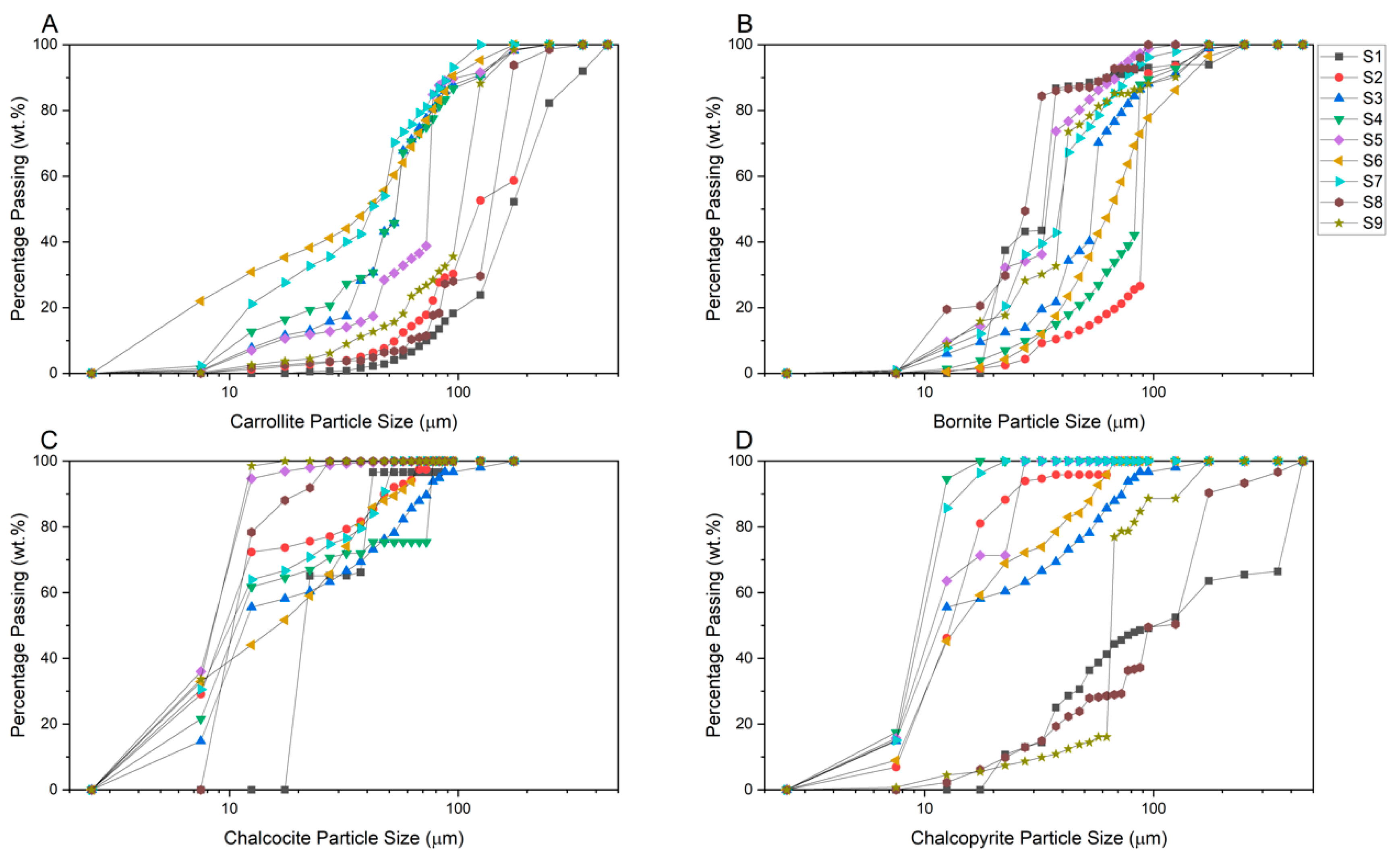
The Particle Size Distribution (PSD) of the target minerals for samples S1 to S9 are shown in Figure 3. It is important to note that in some cases rectangular steps are observed in the data. These are caused by the method through which the particle size data is classified in QEMSCAN data processing software. The PSD will not be smooth if no particles are recorded within that size class. Additionally, the modal mineralogy data from Table 2 needs to be considered when interpreting Figure 3, as negligible mineral content in the feed will mean that the PSD will not provide much information (e.g., bornite and chalcocite in sample S1 and chalcopyrite in samples S4 and S5). The mineral particle sizes vary per mineral and per sample. Sample S1 contains particles of carrollite and chalcopyrite that may not respond to flotation effectively as these will be too coarse [27]. For chalcopyrite, that is also the case for sample S8. There are no samples in which coarse particles of bornite and chalcocite are present. Of the target minerals, chalcocite has the finest particles. When considering the presence of non-valuable minerals (Table 2), it can be seen that the samples with a higher content of silicate minerals (Sample S1 and S8) contain coarser target particles, indicating that the grinding process has been less efficient for these samples.

3.1.3. Feed Liberation and Mineral Association

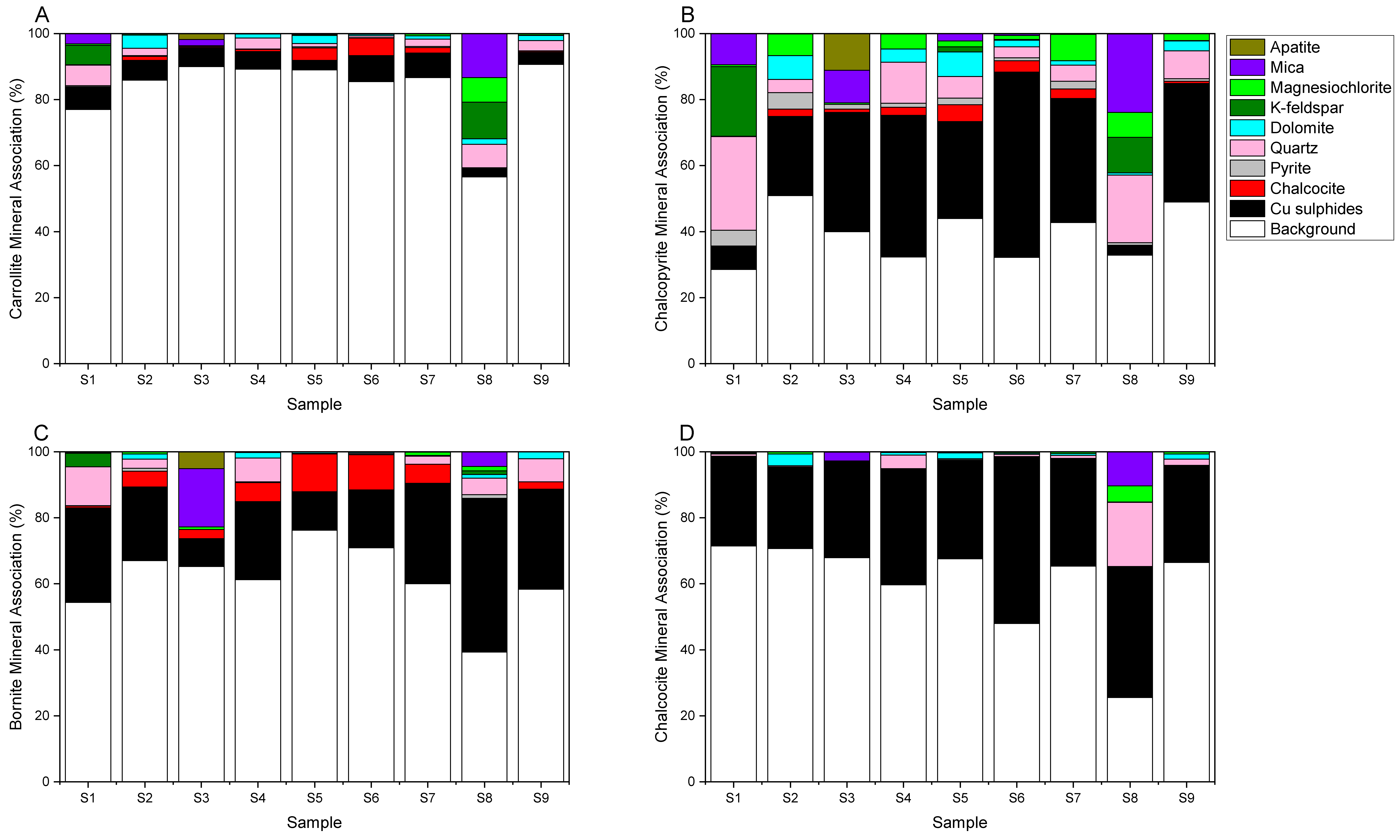
Figure 4 shows the mineral association of the target minerals for samples S1 to S9. When interpreting this data, it is important to consider the mineral abundance in the sample (Table 2). For example, the data for bornite in samples S1 and S8 does not provide much information due to a negligible amount of the mineral being present in the feed. Association of a mineral with the background material can be considered a proxy for liberation as this indicates the average surface area of the mineral that allows for collector adsorption. Additionally, association with other copper sulphide minerals needs to be considered as these also can be available for collector adsorption. Chalcocite is highlighted as well, as the flotation domain of chalcocite does not overlap with the other copper sulphides [28]. Carrollite is mainly associated with the background material and copper sulphides (ranging from 50% in sample S8 and to 96% in sample S3). This association is lower for some of the copper sulphide minerals: for chalcopyrite its association ranges from 36% (sample S1) to 88% (sample S7), for bornite from 74% (sample S3) to 90% (sample S7) and for chalcocite from 65% (sample S8) to 99% (sample S6). For most samples, an association with both quartz and dolomite can be observed. Other minor associations with gangue minerals, include apatite (in sample S3), K-feldspar and muscovite (in sample S1 and sample S8 for carrollite and chalcopyrite). This is explained by a higher presence of those gangue minerals in the identified samples (Table 2).

3.2. Flotation Performance

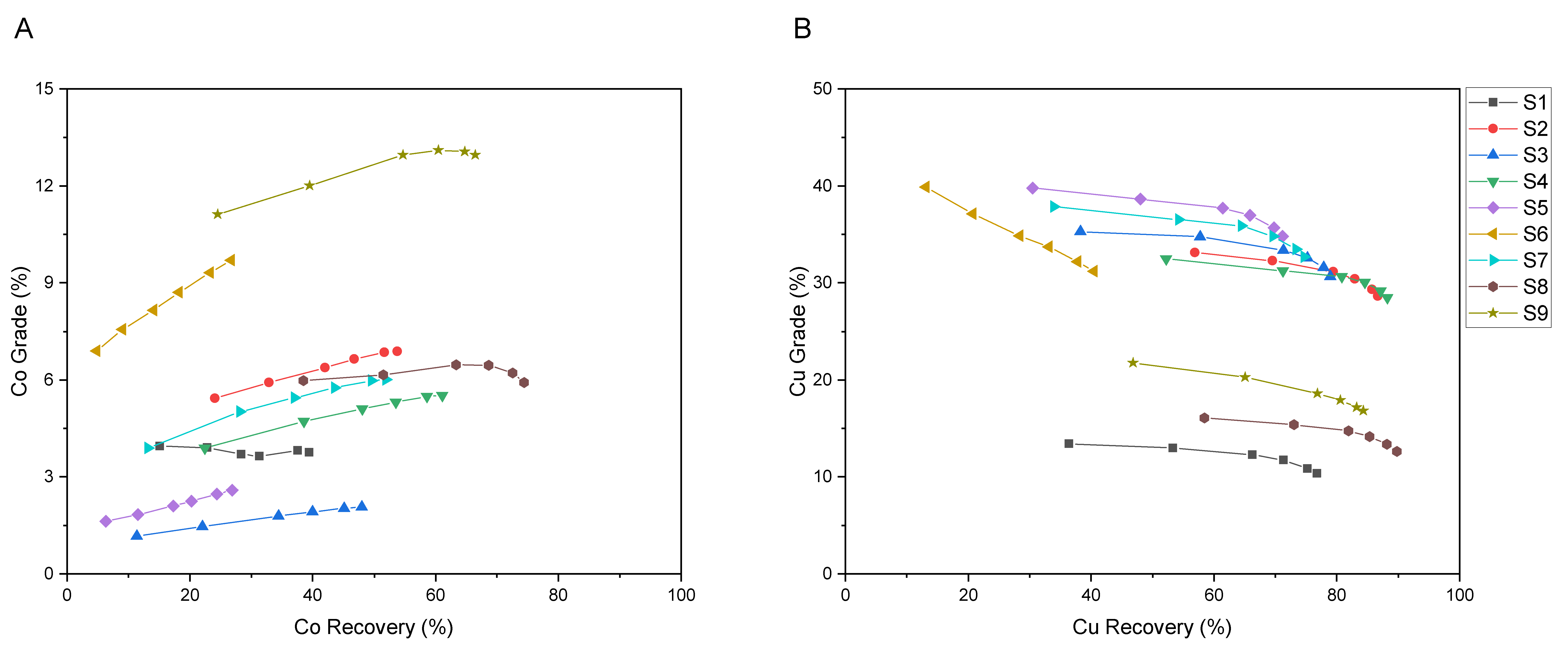
3.2.1. Copper and Cobalt Grade-Recovery Curves

The grade-recovery curves of copper and cobalt for the nine samples are shown in Figure 5. There are differences in the trends of the grade-recovery curves observed for the two metals. For cobalt, in most cases, the initial increase in recovery also leads to an increase in grade. The explanation for this may be that the collector preferentially adsorbs on the surface of copper sulphides, prior to adsorbing onto the surface of the copper–cobalt sulphide mineral carrollite. That means that the copper-bearing particles are initially recovered, followed by carrollite in later stages of the flotation process. For cobalt, the maximum final grade was observed for sample S9 with 13.0% Co and a cobalt recovery of 66.5% while the highest final recovery was observed for sample S8 with 74.4% cobalt recovery and a final grade of 5.9% Co.

For copper however, an increase in recovery comes with a decrease in grade, in line with the usual trend for grade-recovery curves [27]. When analyzing the grade-recovery curves of sample S3, S5 and S7 a common trend can be observed: for the first data points, samples with a higher initial grade, have a lower recovery and samples with a higher initial recovery, have a lower grade. For copper, the maximum final grade was observed for sample S5 with 34.8% Cu and a recovery of 71.2%. The maximum copper recovery was observed for sample S8, with 89.8% copper recovery and a grade of 12.6% Cu. For both copper and cobalt, it can be expected that mineralogical properties have influenced the differences in grade recovery curves. Additionally, for copper, the copper content of the different copper sulphide minerals (Figure 2) may influence the position of the curve.

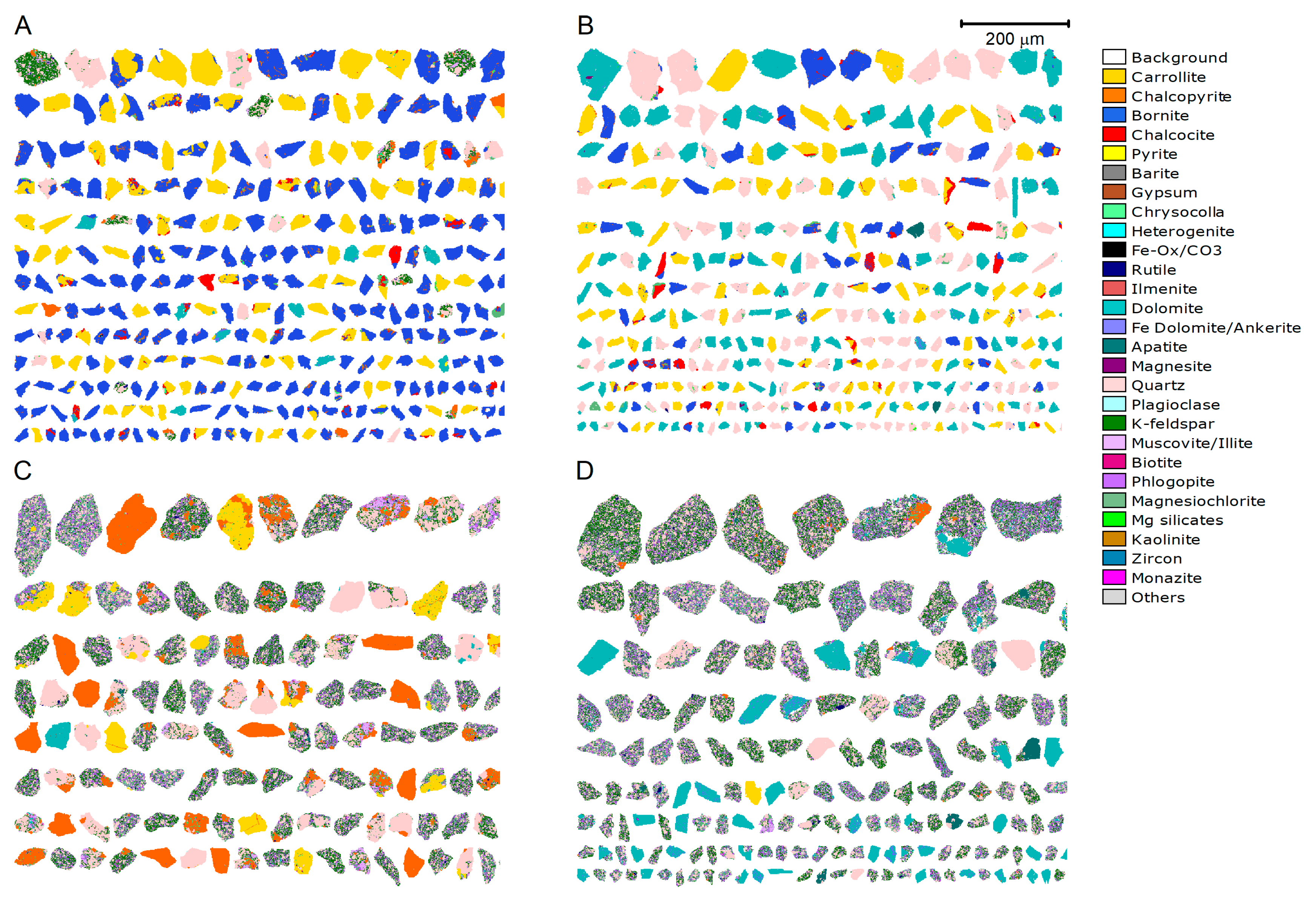
Figure 6 illustrates the differences in composition of the concentrate and tailings from sample S6, which yielded a high Cu-Co grade and lower recoveries (Figure 6A,B), and from sample S8, with a high recovery and lower grade (Figure 6C,D). The flotation concentrate from sample S6 mainly consists of the valuable sulphide minerals bornite, carrollite and minor chalcocite with a relatively small number of gangue particles (quartz, K-feldspar and dolomite). The flotation tailings from sample S6 mainly consist of dolomite and quartz, well-liberated carrollite grains and to a lesser extent bornite and chalcocite grains. This is in line with the lower recovery observed for both copper and cobalt for sample S6. When considering the concentrate and tailings of sample S8, the opposite can be observed. Indeed, in the final tailings of sample S8, one free carrollite grain can be observed and a minor amount of chalcopyrite, as fine grains disseminated in larger particles mainly consisting of gangue minerals. The concentrate obtained with sample S8 contains a larger amount of gangue particles. Approximately half of the particles shown in Figure 6C are made up of gangue minerals, mainly fine-grained silicates (K-feldspar and quartz) with minor amounts of dolomite. Chalcopyrite and carrollite can also be clearly detected, but in a smaller abundance than in the concentrate obtained with sample S6.

3.2.2. Copper and Cobalt Flotation Kinetics

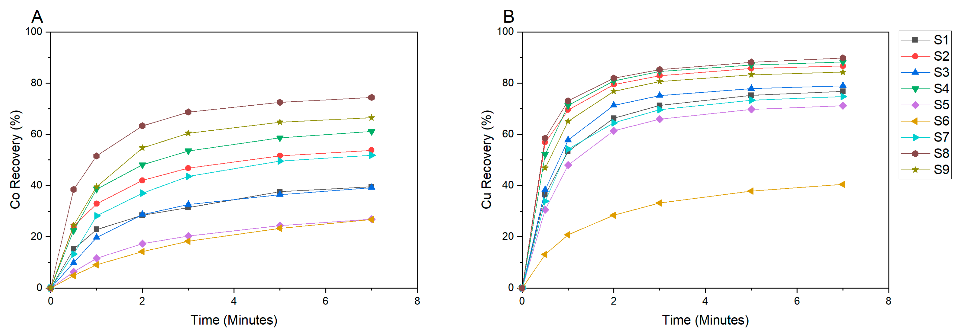
The kinetics curves for cobalt are shown in Figure 7A. A large variability in rougher cobalt recovery is observed, ranging from 27% to 74% Co recovery at equilibrium. The kinetics curves for copper are shown in Figure 7B. Again, a large range of copper recovery is observed, varying from 40% to 90% Cu recovery. The differences in copper recovery between samples are smaller than the differences observed for cobalt recovery. When comparing the trends of cumulative recoveries of the two metals, copper displays faster kinetics than cobalt. Copper recovery after 30 s varies from 13% to 59%, whereas for cobalt the recovery after 30 s ranges between 5% and 38%. In both cases, sample S8 has the highest equilibrium recovery and highest recovery after 30 s, whereas sample S6 displays the lowest equilibrium recovery for both metals. The difference in kinetics between cobalt and copper is in line with what was observed for the grade-recovery curves in Figure 5. Copper tends to be preferentially recovered and the cobalt bearing mineral is recovered later in the flotation process, which leads to a higher equilibrium recovery and faster kinetics for copper.

3.2.3. Fitting of Flotation Models to Metal Recovery Data

Rougher flotation kinetics data, consisting of the six data points of the cumulative metal recovery in Figure 7, have been fitted to the models described in Section 2.3. Curve-fitting statistics of each model and for all the samples can be found in Appendix B, including model precision (R²) and Root Mean Square Error (RMSE). When considering the results for both cobalt and copper, model 2 is the best performing model, as it has the best fitting statistics for six out of the eighteen results. An advantage of selecting the same model for Cu and Co recovery is that it allows for direct comparison of the differences in model parameters between the two metals, being the reason for selecting model 2. The fitted values for kinetics model 2 for copper and cobalt, i.e., kinetic constant value and equilibrium recovery, and the final grade used as response variables in the MLR analysis are shown in

Table 3. Fitted parameters for kinetics model 2 and measured final grades that were used as dependent variables in the Multiple Linear Regression (MLR) analysis.

Flotation Performance Parameters	S1	S2	S3	S4	S5	S6	S7	S8	S9
Co rate constant ($k_2^{Co}$)	1.76	2.20	1.13	1.95	0.95	0.59	1.31	2.96	1.85
Co equilibrium recovery ($R_{eq}^{Co}$)	41.32	56.19	55.33	65.30	31.08	34.63	58.34	77.44	72.84
Co final grade ($G_{final}^{Co}$)	3.76	6.88	2.07	5.53	2.59	9.69	6.00	5.92	12.95
Cu rate constant ($k_2^{Cu}$)	2.69	4.93	2.91	4.15	2.39	1.38	2.71	4.99	3.61
Cu equilibrium recovery $(R_{eq}^{Cu})$	81.21	88.84	84.22	91.79	76.35	44.26	79.31	91.72	88.44
Cu final grade $(G_{final}^{Cu})$	10.37	28.61	30.64	28.50	34.78	31.22	32.68	12.63	16.83

.

3.3. Regression Analysis

To allow for a quantitative investigation into the relationship between the flotation performance of copper and mineralogical data from the four copper containing minerals, a copper deportment weighted average was calculated of the mineralogical parameters. The table with the weighted averages parameters for the Cu minerals can be found in Appendix A. The correlation matrix used to initialize the regression analysis can be found in the Supplementary Material (Table S1).

3.3.1. Selection of Regression Variables

The correlation coefficients as calculated for the variables used in the models for copper and cobalt flotation performance can be found in Appendix C. For the Co model variables, a strong negative correlation was found between the liberation of carrollite and carrollite association with magnesiochlorite. Substitution was investigated, but this caused a decrease in model performance. For the variables used in the copper models, there is a strong positive correlation between bornite and the total percentage of sulphide minerals in the feed. It was investigated whether bornite could replace the sulphide content in the models and whether the sulphide content could replace bornite feed content. Again, this led to a decrease in the R² of the models and the significance of the independent variables.

3.3.2. Multiple Linear Regression Results for Selected Variables

Multiple Linear Regression (MLR) has been applied to the set of selected mineralogical parameters and for each of the dependent variables (i.e., kinetic model parameters and final grade). The summary statistics describing the accuracy of the models for each flotation performance parameter are shown in

Table 4. R², RMSE, F-value and model significance (Prob > F) for the final grade, rate constant and equilibrium recovery of copper and cobalt.

	${\mathit{G}}_{\mathit{f}\mathit{i}\mathit{n}\mathit{a}\mathit{l}}^{\mathit{C}\mathit{u}}$	${\mathit{R}}_{\mathit{e}\mathit{q}}^{\mathit{C}\mathit{u}}$	${\mathit{k}}_2^{\mathit{C}\mathit{u}}$	${\mathit{G}}_{\mathit{f}\mathit{i}\mathit{n}\mathit{a}\mathit{l}}^{\mathit{C}\mathit{o}}$	${\mathit{R}}_{\mathit{e}\mathit{q}}^{\mathit{C}\mathit{o}}$	${\mathit{k}}_2^{\mathit{C}\mathit{o}}$
R2	0.98	0.95	0.99	0.93	0.97	>0.99
RMSE	3.74	4.29	0.17	2.48	3.99	0.04
F-value	47.77	29.69	105.69	23.95	32.17	633.98
Prob > F	<0.01	<0.01	<0.01	<0.01	<0.01	<0.01

. The significance of each model is very high for each parameter, as in all cases Prob > F is smaller than 0.01. The Root Mean Square Errors are quite low for most models. For the models dealing with higher values, such as the equilibrium recovery and final grades of both copper and cobalt, also higher errors are observed. The results for cobalt are overall better than for copper, when considering the rate constant and equilibrium recovery models. Of the final grade models, the cobalt model has the lowest R². The experimental error is not included in these statistics. It can be expected that including such an error, assuming that the error is systematic, will lead to an offset in the statistics for all six models.

Results for each dependent variable in terms of regression coefficients, standard error, t-value and significance (Prob > |t|) of the independent variables are shown in

Table 5. Intercept and mineralogical parameters that influence the final grade, rate constant and equilibrium recovery of copper and cobalt.

Model Parameter	Variable	Value	Standard Error	t-Value	Prob > |t|
$G_{final}^{Cu}$	Intercept	28.64	2.23	12.82	<0.01
	Chalcocite content (%Cc)	10.30	2.17	4.71	0.01
	Carrollite content (%Car)	−9.67	2.28	−4.24	0.01
	Bornite content (%Bn)	6.68	2.45	2.72	0.05
	Cu sulphide F100 (Cu F100)	−17.06	2.72	6.26	<0.01
$R_{eq}^{Cu}$	Intercept	114.13	4.44	25.69	<0.01
	Chalcocite content (%Cc)	−20.24	5.04	−4.01	0.01
	Total sulphide content (%Sul)	−49.22	7.55	−6.52	<0.01
	Cu sulphide F100 (Cu F100)	−29.36	5.83	−5.04	<0.01
$k_2^{Cu}$	Intercept	2.98	0.14	21.39	<0.01
	Chalcocite content (%Cc)	−1.13	0.19	−6.03	<0.01
	Carrollite content (%Car)	−1.23	0.22	−5.54	0.01
	Cu MA dolomite (Cu MA Dol)	2.34	0.17	13.97	<0.01
	Cu MA magnesiochlorite (Cu MA Mgc)	1.20	0.22	5.35	0.01
$G_{final}^{Co}$	Intercept	5.82	1.06	5.48	<0.01
	Chalcocite content (%Cc)	−5.08	1.23	−5.12	0.01
	Carrollite content (%Car)	12.20	1.46	8.33	<0.01
	Carrollite liberation (Car lib)	−4.82	1.54	−3.13	0.03
$R_{eq}^{Co}$	Intercept	66.77	2.82	23.68	<0.01
	Chalcocite content (%Cc)	−42.17	4.61	−9.16	<0.01
	Carrollite F100 (Car F100)	−28.18	4.88	−5.78	<0.01
	Carrollite MA magnesiochlorite (Car MA Mgc)	31.39	5.30	5.92	<0.01
	Carrollite MA dolomite (Car MA Dol)	13.81	4.59	3.01	0.04
$k_2^{Co}$	Intercept	2.91	0.05	56.83	<0.01
	Chalcocite content (%Cc)	−1.42	0.05	−29.61	<0.01
	Magnesiochlorite content (%Mgc)	−0.51	0.04	−11.72	<0.01
	Carrollite liberation (Car lib)	−1.35	0.05	−26.52	<0.01
	Carrollite MA dolomite (Car MA Dol)	1.16	0.05	23.07	<0.01

. As discussed in Section 2.4.1, the independent variables were normalized allowing for an equal comparison between the regression coefficients of the independent variables. The final grade of copper is shown to be influenced by the presence of chalcocite (+10.30), carrollite (−9.67) and bornite (+6.68) in the feed and by the fraction of copper sulphide minerals larger than 100 µm (−17.06), defined as Cu F₁₀₀. The intercept is set at 28.64%. This means that when there is no bornite or chalcocite present in the feed, a final grade of 28.64% is expected, for the experimental domain covered in this study. The equilibrium copper recovery has been linked to three parameters: chalcocite content (−20.24), total sulphides in the feed (−49.22) and the fraction of copper sulphide minerals larger than 100 µm (−29.36). The intercept is 114.14%, which explains why all the parameters have a negative coefficient. Four mineralogical parameters have been identified to influence the copper rate constant: chalcocite content (−1.13), carrollite content (−1.23), the association of copper bearing minerals with dolomite (+2.34) and association of copper bearing minerals with magnesiochlorite (+1.20).

For cobalt, three parameters were identified to influence the final grade: carrollite content (+12.20), chalcocite content (-5.08) and the liberation of carrollite (−4.82). The equilibrium recovery of cobalt has been linked to two negative parameters and two positive parameters. The negative parameters are the chalcocite content (−42.17) and the fraction of carrollite particles that are larger than 100 μm (−28.18), defined as defined as Car F₁₀₀. Two positive parameters are the association of carrollite with magnesiochlorite (+31.39) and association of carrollite with dolomite (+13.81). For the rate constant of cobalt, one positive factor was identified and three variables with a negative coefficient. The positive factor is the association of carrollite with dolomite (+1.16). The three negative factors are chalcocite content (−1.42), magnesiochlorite content (−0.51) and the average liberation of carrollite (−1.35).

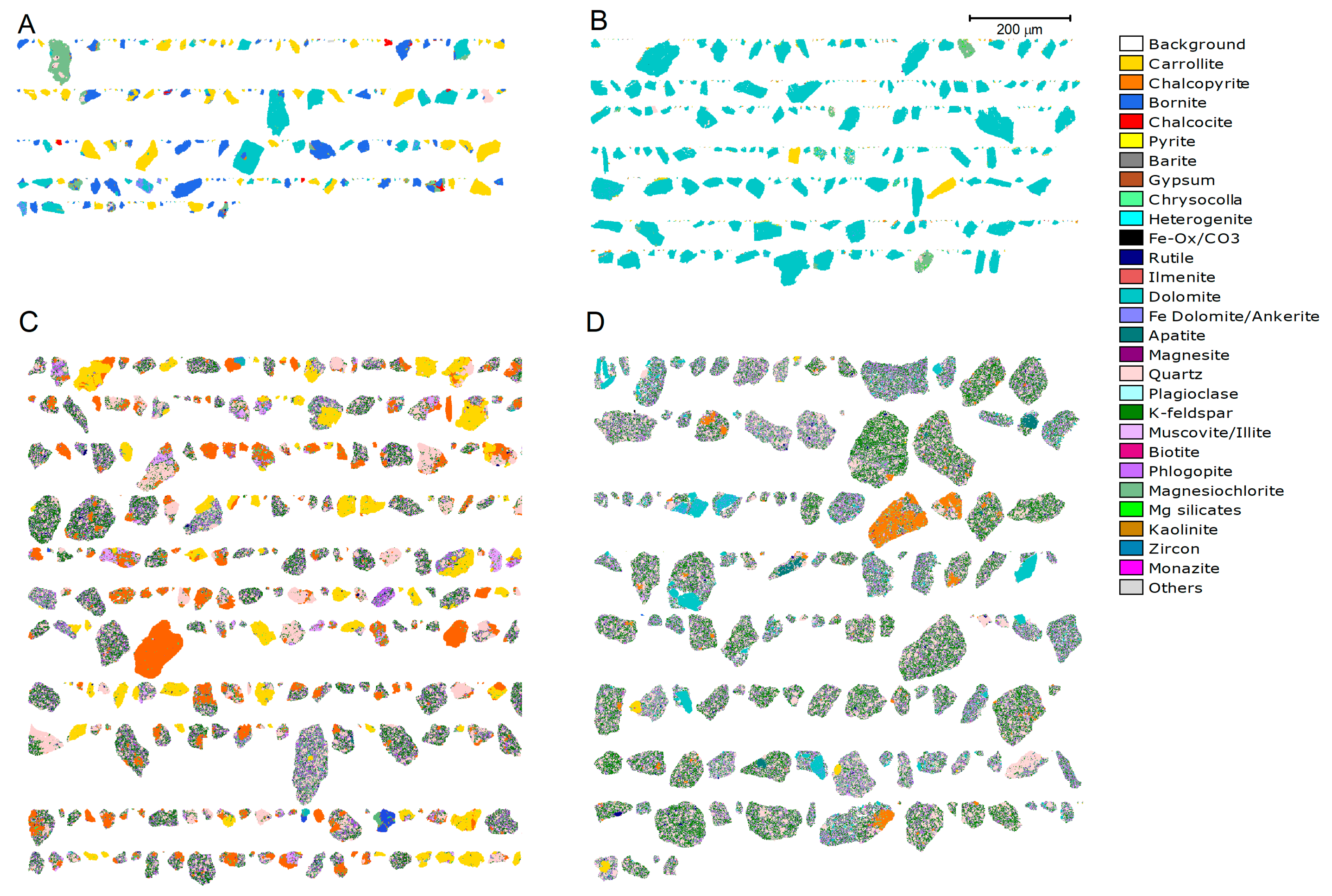
Chalcocite feed content is found as a factor of influence, both positive and negative, for all models. Both chalcocite and pyrite are known to depress the flotation of copper-bearing sulphide minerals due to galvanic passivation [29,30,31]. In this case, it is possible that the pyrite content in the feed is not high enough for galvanic passivation to take place. In another study, a minimum of 20% of pyrite was added in order to investigate the influence of pyrite content on chalcopyrite flotation behavior [32]. The highest percentage of pyrite found in the feed samples of this study is 1% (Table 2). The equilibrium recovery of copper is negatively influenced by the percentage of sulphide minerals in the feed. It has been shown that base metal sulphides have an effect on the mineral surface hydrophobicity through the formation of hydrophilic oxidation products [29,30,33]. A higher grade of sulphide minerals will cause more surface oxidation and thus reduces the eventual equilibrium recovery. An increase in the grade of the copper minerals leads to an increase in the final copper grade, whilst an increase in the later recovered carrollite and coarse particles leads to a decrease in copper grade. The strong influence of carrollite content on the final cobalt grade is logical as well, as carrollite was identified as the single cobalt carrying mineral in the feed samples. The negative influence of an increase in particles of Cu and Co minerals larger than 100 µm in the feed is in line with expectations. The proportion of particles that cannot be effectively separated increases as the mineral particle size of the valuable minerals increases beyond a threshold value [27]. This causes a decrease in equilibrium recovery and final Cu grade. The positive influence of magnesiochlorite on the cobalt rate constant is more difficult to understand. It is probable that magnesiochlorite content represents a combination of other variables that positively influence the rate constant. The negative impact of an increase in carrollite liberation on the final cobalt grade and cobalt rate constant indicates that a decrease in association with other particles (e.g., Cu sulphides) leads to a later recovery of the Co particles in the flotation process. It is more difficult to understand the positive correlation between association of carrollite and copper sulphide minerals with dolomite and magnesiochlorite on the copper rate constant, cobalt equilibrium recovery and cobalt rate constant. To evaluate whether the association of the target minerals with dolomite and magnesiochlorite indeed has a positive influence, the target minerals particles in the concentrate and tailings of the samples with the highest association with magnesiochlorite (sample S8) and dolomite (sample S2) were compared. The concentrates and tailings of these samples are shown in Figure 8. The sulphide particles in the concentrate of samples S2 have a lower association with dolomite than the particles in the tailings (6.6% vs. 21.5%). For sample S8, the sulphide particles in the concentrate on average also have a lower association with magnesiochlorite than the sulphide particles in the tailings (3.7% vs. 8.6%). These results show that the positive effect of dolomite and magnesiochlorite association with the target minerals is likely to be a consequence of more complex combinations of other particulate parameters that do have a positive effect on the flotation performance. Note that the intercept of the copper equilibrium recovery is 114.13%, meaning that if there are no copper sulphides present in the feed (all parameters equal to zero), this model would give a recovery of over a 100%. While this may appear unrealistic, one should remind that regression models are only valid for the experimental domain defined by the dataset provided for the regression, i.e., the multivariate space represented by all the variables and their extreme boundaries. In this case study, the situation where all input parameters are equal to zero is never met. Hence, the predicted recovery never goes over 100%. This observation just shows, as in any regression model, the limitation of the MLR method.

3.3.3. Regression Models Cross Validation

The correlation between predicted and observed values for the copper and cobalt rate constant, equilibrium recovery, final grade and metal recovery with time are shown in Figure 9. The RMSECV is calculated using Equation (8). The models for predicting the Cu and Co grade come with an R² of 0.93 and 0.80 and RMSECV of 1.34% and 4.41% respectively. The RMSECV is higher for the copper grade model as that model needs to deal with higher values. For both copper and cobalt, there is a strong correlation between the predicted and measured values of the rate constant. For cobalt, the model has an RMSECV smaller than 0.07 and an R² of 0.99. The relationship between the observed and predicted values is linear. For the copper rate constant, the RMSECV is 0.30 and has an R² of 0.94. For both the copper and cobalt rate constant, the predicted and observed values are well spread out. The observed and predicted values for the equilibrium recovery of cobalt and copper are in good agreement, with an R² of 0.87 and test error of 6.15% for cobalt and 0.86 and 6.22% for copper, respectively. The values of the copper equilibrium recovery are grouped together above a recovery of 80%, with only one sample having a lower recovery. This is a weakness of the model, as it may lead to larger errors when predicting the equilibrium recovery of samples between 45% and 75%. The metal recovery with time can be predicted when inserting the predicted rate constant values and equilibrium recovery in Equation (3). For cobalt, the recovery model has an R² of 0.94 and RMSECV of 4.70% whilst, for copper, the model has an R² of 0.94 and RMSECV of 5.14%.

3.4. Model Limitations and Further Development

While this study has yielded interesting results with good prediction performance, the obtained models cannot be used for direct prediction of flotation performance industrially as some limitations exist. First, it should be noted that these models are deposit-specific and that the copper and cobalt flotation models can be used for predictive purposes for the investigated deposit specifically and for samples displaying mineral grades and mineralogical properties within the range of those covered in this study. If additional zones are discovered within the deposit with varying mineralogy, outside the investigated experimental domain, these models may change. In this case, additional data points would be required to strengthen the statistical reliability of the models for industrial-scale application. Replicate experiments, which could not be performed for most samples in this study due to lack of quantity, will also be required to provide insight into the overall model’s stability. However, as a proof of concept, it has been shown that it is possible to predict flotation performance from basic mineralogical data. Such models are of great value from a geometallurgical perspective, as it has the potential to include flotation performance in the geometallurgical model from mineralogical core data. The possibilities of this approach can be expanded further by performing additional experiments where operating conditions are varied, such as the addition of a depressant or modifier, variation in collector dosage, account for changes in water quality and adjustment of the aeration rate for optimum separation of valuable and gangue material. In order to understand the applicability of these models on an industrial scale, it is also important to consider the operational differences between laboratory bench scale and industrial steady state operations [34]. Addressing all these factors will lead to more robust models which could assist process operators in deciding what to change in the flotation circuit to minimize the impact of varying mineralogy on copper and cobalt flotation performance.

4. Conclusions

In this paper, flotation performance of copper and cobalt was linked to fundamental mineralogical data obtained from a standardized flotation batch experiment. The flotation kinetics of copper and cobalt was well fitted by a first-order rectangular distribution model, delivering flotation performance indexes obtained from experimental data. The rate constant, equilibrium recovery and final grade of copper and cobalt were correlated with quantitative mineralogical data from QEMSCAN through Multiple Linear Regression. It was shown that the flotation performance could be correlated to the total sulphide, carrollite, bornite, chalcocite and magnesiochlorite content in the feed. Other mineralogical factors that were found to be significant were the liberation of carrollite, the percentage of copper and cobalt mineral particles above 100 μm and association of the copper and cobalt minerals with magnesiochlorite and dolomite. LOOCV was used to determine the predictability of the models. For both copper and cobalt, the predictability of the final grade showed a RMSECV and R² of 1.34% and 0.93 for cobalt and 4.41% and 0.80 for copper. By combining the predicted rate constant and equilibrium recovery, the recovery with time could be predicted for both metals. This model had an overall test error and R² of 4.70%, respectively 0.94 for cobalt and 5.14% and 0.94 for copper. While the predictive flotation performance models are deposit-specific and require calibration for each deposit, the workflow described in this study represents a proof-of-concept suitable for geometallurgical application, where combining laboratory experiments with quantitative mineralogy will allow to refine the prediction of flotation performance on an industrial scale.

References

- Lund, C.; Lamberg, P. Geometallurgy-A tool for better resource efficiency. Eur. Geol. 2014, 37, 39–43. [Google Scholar]
- Dehaine, Q.; Filippov, L.O.; Glass, H.J.; Rollinson, G. Rare-metal granites as a potential source of critical metals: A geometallurgical case study. Ore Geol. Rev. 2019, 104, 384–402. [Google Scholar] [CrossRef] [Green Version]
- Alruiz, O.M.; Morrell, S.; Suazo, C.J.; Naranjo, A. A novel approach to the geometallurgical modelling of the Collahuasi grinding circuit. Miner. Eng. 2009, 22, 1060–1067. [Google Scholar] [CrossRef]
- Navarra, A.; Grammatikopoulos, T.; Waters, K. Incorporation of geometallurgical modelling into long-term production planning. Miner. Eng. 2018, 120, 118–126. [Google Scholar] [CrossRef] [Green Version]
- Lamberg, P. Particles–the bridge between geology and metallurgy. In Proceedings of the Conference in Mineral Engineering, Luleå, Sweden, 8–9 February 2011; pp. 1–16. [Google Scholar]
- Schmidt, T.; Buchert, M.; Schebek, L. Investigation of the primary production routes of nickel and cobalt products used for Li-ion batteries. Resour. Conserv. Recycl. 2016, 112, 107–122. [Google Scholar] [CrossRef]
- Fisher, K.G.; Treadgold, L.G. Design Considerations for the Cobalt Recovery Circuit of the Kol (Kov) Copper/Cobalt Refinery, DRC. In Proceedings of the ALTA Nickel-Cobalt Conference, Perth, Australia, 25–27 May 2009. [Google Scholar]
- Crundwell, F.K.; Moats, M.S.; Ramachandran, V.; Robinson, T.G.; Davenport, W.G.; Crundwell, F.K.; Moats, M.S.; Ramachandran, V.; Robinson, T.G.; Davenport, W.G. Production of Cobalt from the Copper–Cobalt Ores of the Central African Copperbelt. In Extractive Metallurgy of Nickel, Cobalt and Platinum Group Metals; Elsevier: Amsterdam, The Netherlands, 2011; pp. 377–391. ISBN 9780080968094. [Google Scholar]
- Mainza, A.N.; Simukanga, S.; Witika, L.K. Technical note evaluating the performance of new collectors on feed to Nkana concentrator’s flotation circuit. Miner. Eng. 1999, 12, 571–577. [Google Scholar] [CrossRef]
- Musuku, B. Enhancing the Recoveries and Grades of Cobalt from Nchanga and Konkola Ores of KCM. Master’s Thesis, University of Zambia, Lusaka, Zambia, 2011. [Google Scholar]
- Tijsseling, L.T.; Dehaine, Q.; Rollinson, G.K.; Glass, H.J. Flotation of mixed oxide sulphide copper-cobalt minerals using xanthate, dithiophosphate, thiocarbamate and blended collector. Miner. Eng. 2019, 138, 246–256. [Google Scholar] [CrossRef]
- Lamberg, P.; Rosenkranz, J. Systematic diagnosis of flotation circuit performance based on process mineralogical methods. In Proceedings of the 14th International Mineral Processing Symposium, Kuşadası, Turkey, 15–17 October 2014; pp. 417–423. [Google Scholar]
- Keeney, L. The Development of a Novel Method for Integrating Geometallurgical Mapping and Orebody Modelling. Ph.D. Thesis, The University of Queensland, Brisbane, Australia, 2010. [Google Scholar]
- Gharai, M.; Venugopal, R. Modeling of flotation process-An overview of different approaches. Miner. Process. Extr. Metall. Rev. 2016, 37, 120–133. [Google Scholar] [CrossRef]
- Whiteman, E.; Lotter, N.O.; Amos, S.R. Process mineralogy as a predictive tool for flowsheet design to advance the Kamoa project. Miner. Eng. 2016, 96–97, 185–193. [Google Scholar] [CrossRef]
- Rincon, J.; Gaydardzhiev, S.; Stamenov, L. Investigation on the flotation recovery of copper sulphosalts through an integrated mineralogical approach. Miner. Eng. 2019, 130, 36–47. [Google Scholar] [CrossRef]
- Little, L.; Mclennan, Q.; Prinsloo, A.; Muchima, K.; Kaputula, B.; Siame, C. Relationship between ore mineralogy and copper recovery across different processing circuits at Kansanshi mine. J. S. Afr. Inst. Min. Metall. 2018, 118, 1155–1162. [Google Scholar] [CrossRef]
- Anderson, K.F.E.; Wall, F.; Rollinson, G.K.; Moon, C.J. Quantitative mineralogical and chemical assessment of the Nkout iron ore deposit, Southern Cameroon. Ore Geol. Rev. 2014, 62, 25–39. [Google Scholar] [CrossRef]
- Gottlieb, P.; Wilkie, G.; Sutherland, D.; Ho-Tun, E.; Suthers, S.; Perera, K.; Jenkins, B.; Spencer, S.; Butcher, A.; Rayner, J. Using Quantitaive Electron Microscopy for Process Mineralogy Applications. J. Miner. Met. Mater. Soc. 2000, 52, 24–25. [Google Scholar] [CrossRef]
- Pirrie, D.; Butcher, A.R.; Power, M.R.; Gottlieb, P.; Miller, G.L. Rapid quantitative mineral and phase analysis using automated scanning electron microscopy (QemSCAN); potential applications in forensic geoscience. Geol. Soc. London Spec. Publ. 2004, 232, 123–136. [Google Scholar] [CrossRef]
- Rollinson, G.K.; Andersen, J.C.Ø.; Stickland, R.J.; Boni, M.; Fairhurst, R. Characterisation of non-sulphide zinc deposits using QEMSCAN®. Miner. Eng. 2011, 24, 778–787. [Google Scholar] [CrossRef]
- Bu, X.; Xie, G.; Peng, Y.; Ge, L.; Ni, C. Kinetics of flotation. Order of process, rate constant distribution and ultimate recovery. Physicochem. Probl. Miner. Process. 2017, 53, 342–365. [Google Scholar]
- Garcia-Zungina, H. The efficiency obtained by flotation is an exponential function of time. Bol. Min. 1935, 47, 83–86. [Google Scholar]
- Klimpel, R.R. Selection of Chemical Reagents for Flotation. Organ. Soc. Min. Metall. Explor. 1980, 2, 907–934. [Google Scholar]
- Arbiter, N. Flotation rates and flotation efficiency. Trans. AIME. Sept. 1951, 791, 796. [Google Scholar]
- James, G.; Witten, D.; Hastie, T.; Tibshirani, R. An Introduction to Statistical Learning; Springer: New York, NY, USA, 2013; ISBN 978-1-4614-7137-0. [Google Scholar]
- Wills, B.A.; Finch, J.A. Wills’ Mineral Processing Technology an Introduction to the Practical Aspects; Butterworth-Heinemann: Oxford, UK, 2016; ISBN 9780080970530. [Google Scholar]
- Lotter, N.O.; Bradshaw, D.J.; Barnes, A.R. Classification of the Major Copper Sulphides into semiconductor types, and associated flotation characteristics. Miner. Eng. 2016, 96–97, 177–184. [Google Scholar] [CrossRef]
- Guy, P.J.; Trahar, W.J. The effects of oxidation and mineral interaction on sulphide flotation. In Flotation of Sulphide Minerals; Stiftelsen Mineral Teknisk Forshning: Stockholm, Sweden, 1985; pp. 91–103. [Google Scholar]
- Trahar, W.J.; Senior, G.D.; Shannon, L.K. Interactions between sulphide minerals-the collectorless flotation of pyrite. Int. J. Miner. Process. 1994, 40, 287–321. [Google Scholar] [CrossRef]
- Owusu, C.; Addai-Mensah, J.; Fornasiero, D.; Zanin, M. Estimating the electrochemical reactivity of pyrite ores-their impact on pulp chemistry and chalcopyrite flotation behaviour. Adv. Powder Technol. 2013, 24, 801–809. [Google Scholar] [CrossRef]
- Owusu, C.; Brito, E.; Abreu, S.; Skinner, W.; Addai-Mensah, J.; Zanin, M. The influence of pyrite content on the flotation of chalcopyrite/pyrite mixtures. Miner. Eng. 2014, 55, 87–95. [Google Scholar] [CrossRef]
- Woods, R. Electrochemical potential controlling flotation. Int. J. Miner. Process. 2003, 72, 151–162. [Google Scholar] [CrossRef]
- Mesa, D.; Brito-Parada, P.R. Scale-up in froth flotation: A state-of-the-art review. Sep. Purif. Technol. 2019, 210, 950–962. [Google Scholar] [CrossRef]
Figure 1.
Overview of the methodology used in this study.
Figure 2.
Copper deportment between the four target sulphide minerals for all samples.
Figure 3.
Particle size distribution of the four target sulphide minerals, i.e., carrollite (A), bornite (B), chalcocite (C), and chalcopyrite (D) for all samples.
Figure 4.
Mineral association of the four target sulphide minerals, i.e., carrollite (A), chalcopyrite (B), bornite (C), and chalcocite (D) for all samples.
Figure 5.
Grade-recovery curves of cobalt (A) and copper (B) for all samples.
Figure 6.
False color QEMSCAN particle mineral maps illustrating flotation concentrates and tailings composition. Typical high grade-low recovery concentrate (A) and associate tailings (B) obtained with sample S6. Typical low grade-high recovery concentrate (C) and associate tailings (D) obtained with sample S8.
Figure 7.
Kinetics curves of cobalt (A) and copper (B) in the rougher stage for all samples.
Figure 8.
False color QEMSCAN particle mineral maps illustrating target minerals associations with dolomite from sample S2 flotation concentrate (A) and tailings (B), and magnesiochlorite from sample S8 flotation concentrate (C) and tailings (D).
Figure 9.
Predicted versus measured values for the Co and Cu final grade (A,B), kinetics model parameters, i.e., rate constant (C,D), equilibrium recovery (E,F) and recovery with time (G,H).