Article

Analytical Model to Compare and Select Creep Constitutive Equation for Stress Relief Investigation during Heat Treatment in Ferritic Welded Structure

1
Department of Mechanical Engineering, Tsinghua University, Beijing 100084, China
2
State Key Laboratory of Tribology, Tsinghua University, Beijing 100084, China
3
Collaborative Innovation Center of Advanced Nuclear Energy Technology, Beijing 100084, China
*
Author to whom correspondence should be addressed.
Metals 2020, 10(5), 688; https://doi.org/10.3390/met10050688
Submission received: 9 April 2020 / Revised: 17 May 2020 / Accepted: 21 May 2020 / Published: 23 May 2020
(This article belongs to the Special Issue Heat Treatment of Steels)

Abstract

:
The one-dimensional analytical model was promoted to help select the creep constitutive equation and predict heat treatment temperature in a ferritic welded structure, along with neglecting the impact of structural constraint and deformation compatibility. The analytical solutions were compared with simulation results, which were validated with experimental measurements in a ferritic welded rotor. The as-welded and post weld heat treatment (PWHT) residual stresses on the inner and outer cylindrical surfaces were measured with the hole-drilling method (HDM) for validation. Based on the one-dimensional analytical model, different effects of Norton and Norton-Bailey creep constitutive equation on stress relief during heat treatment in a ferritic welded rotor were investigated.

1. Introduction

Welding is widely used in the connection and manufacturing of thick-walled heavy mechanical components, considering the restraint of forging capacity and flexibility in design and fabricating [1]. However, due to the nonuniform heating and cooling processes encountered during welding, residual stress is bound to be generated in welded joints, which affects the yield strength [2,3], fatigue strength [4,5], and creep properties [6,7]. Heat treatment is an important approach to eliminate residual stress in large-scaled and heavy components. Nevertheless, it is expensive and inefficient to find the optimum heat treatment through an experimental measurement of residual stress. Thus, numerical simulation is widely employed to calculate the residual stress. The stress relief during heat treatment is considered as an effect of creep behavior [8], which can be estimated with creep constitutive equations [8,9,10]. The Norton equation or Norton-Bailey equation were widely employed in many researches [11,12,13]. It is found through an experiment that the Norton equation and Norton-Bailey equation have the same effect on eliminating residual stress at high temperatures [14]. However, there is a lack of detailed investigations on the different effects of Norton and Norton-Bailey equation on stress relief at different temperatures. In addition, the specific mechanism for the substitutability of creep equations at high temperatures is not clear and it is important to obtain the demarcation temperature, at which the two equations have substitutability in order to help select the appropriate creep equation in simulation depending on the employed PWHT temperature. Nevertheless, it is expensive and inefficient to obtain the demarcation temperature experimentally, which calls for another efficient method.
In this study, the one-dimensional analytical model was promoted to investigate the different effects of Norton and Norton-Bailey creep constitutive equation on stress relief during heat treatment in a ferritic welded rotor. The analytical solutions were compared with simulation results, which were validated with experimental measurements. It is found that the analytical model can be helpful to select the creep constitutive equation and predict the appropriate range of heat treatment temperature conveniently.

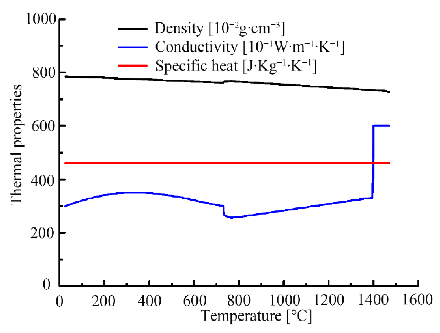
2. Material Properties

The base metal of welded ferritic rotor is 25Cr2Ni2MoV steel and its chemical compositions are listed in Table 1. The weld metal is similar to 25Cr2Ni2MoV steel in terms of chemical compositions and the same material property will be employed in simulation for the base metal and the weld metal. The material properties were measured experimentally, preparing for thermal analysis, mechanical analysis, and stress relief analysis corresponding to the welding process and heat treatment.
Thermal properties are shown in Figure 1, obtained with the JMatPro software (version 7.0, Sente Software Ltd., Guildford, UK). Figure 2 presents the shape and dimensions of the creep test specimens and tensile test specimens. Uniaxial tensile tests were conducted at temperatures from 25 to 850 °C. Phase transformation during the heating and cooling process was considered. A portion of tensile test specimens were heated up to 850 °C and cooled to the test temperature to obtain the microstructure corresponding to the cooling process before conducting a tensile test. Mechanical properties for the mechanical analysis are listed in Figure 3 and properties over 850 °C were inferred. The thermal strain in Figure 3a is composed of a thermal expansion and expansion from phase transformation. It is obvious that phase transformation occurred in the process of heating up and cooling down. The linear isotropic hardening rule was employed in the investigation.
Creep occurs at temperatures around and over 0.4 T m [15], where T m corresponds to the melting temperature. The melting temperature of 25Cr2Ni2MoV is approximately 1360 °C. It is indicated that the stagnation temperature of 25Cr2Ni2MoV to creep is approximately 380 °C. It is also reported that parts of M/A constituents were deposited into an accumulated carbide at 650 °C [16]. Therefore, creep tests were carried out at 500, 560, 600, and 630 °C, preventing the M/A constituent deposition. Table 2 lists the conditions for creep tests. Material coefficients of the Norton equation and Norton-Bailey equation were extracted from experimental creep strain-time data, neglecting diffusional creep. The Norton equation is written as follows:
ε ˙ m = A σ n
where ε ˙ m refers to the minimum creep rate and σ is the effective stress in the specimen. The coefficients A and n are listed in Table 3. The Norton-Bailey equation is written as follows:
ε ˙ c r = B σ u t m
where ε ˙ c r refers to the creep rate and t is the total creep time. The coefficients B , u , and m are also listed in Table 3.

3. One-Dimensional Analytical Model and Analytical Solutions

The dominant mechanism for stress relief in ferritic steel is creep strain relaxation and a little plastic strain occurs during the heat treatment [8]. Based on the creep strain relaxation mechanism, differences between Norton-Bailey and Norton equation in stress relaxation can be analyzed. The one-dimensional analytical model was promoted to neglect the impact of structural constraint and deformation compatibility, as shown in Figure 4. The simplified model was heated to a preset temperature T °C and a predetermined load σ was applied. Then, the end position was constrained and the stress inside was residual stress, which would be released with creeping at T °C. After sufficient heat treatment, the creep rate ε ˙ in any part was small enough that the creep strain under the action of finite time t was small and negligible, that is:
ε ˙ t 1 /
The small creep rate was denoted as ε ˙ 0 . According to Equation (1), the residual stress after heat treatment under Norton equation in the one-dimensional analytical model ( σ p n ) was solved as follows:
σ p n = ( ε ˙ 0 / A ) 1 / n ( σ σ p n )
Creep strain relaxation mechanism during heat treatment could be described as follows:
d σ = E d ε c r
Combining Equations (1) and (5), the time required was formulated as follows:
t n = σ 1 n σ p n 1 n ( 1 n ) E A ( σ σ p n )
Similarly, the residual stress after heat treatment under Norton-Bailey equation in the one-dimensional analytical model ( σ p b ) could be solved according to Equations (2) and (5). The Norton-Bailey equation was rewritten in the form of strain-hardening, as illustrated in Figure 4b. The shaded region referred to the accumulated creep strain ε c r . The equation in the form of strain hardening was as follows:
ε ˙ c r = ( B σ u ) 1 1 m [ ( 1 m ) ε c r ] m 1 m
Then, the residual stress could be described as follows:
σ = σ p b + E 1 m ( B σ p b u ) 1 m ( ε ˙ 0 ) 1 m m
The time required could also be formulated as follows:
t b = [ 1 m ( 1 u ) E B ( σ 1 u σ p b 1 u ) ] 1 1 m
Considering the engineering practice, the finite time for a negligible creep strain could be set as t t h r = 20   h . Taking the availability of stress relief into consideration, the deviation of stress relief at room temperature was set as σ t h r 10   MPa . Therefore, ε ˙ 0 could be obtained.
ε ˙ 0 = σ t h r / ( E · t t h r ) = 2.4 × 10 6 / h
Based on Equations (4) and (8), the relationship between initial residual stress and PWHT residual stress under the control of Norton equation and Norton-Bailey equation can be obtained easily, which can help select the creep constitutive equation and predict the proper range of heat treatment temperature in a ferritic welded structure.
According to Equations (4) and (8), Figure 5 presents the relationship between initial stress σ and PWHT stress with Norton and Norton-Bailey equations in the one-dimensional analytical model. It indicates that stress relief will not occur when the initial stress is lower than σ p n under Norton equation. When the initial stress is higher than σ p n , the PWHT residual stress is the same, being σ p n with Norton equation. Meanwhile, there is a positive correlation between PWHT residual stress and initial stress with Norton-Bailey equation being higher. It can be explained with the evolution of a dislocation structure and free dislocation density during heat treatment. In the process of stress relief by creep strain, a higher stress is required to obtain the same creep rate with dislocation entanglement and free dislocation density reduction, which means a greater creep resistance. On the other hand, creep strain releases stress, which weakens the driving force of creep. If the PWHT residual stress is the same, a greater creep strain corresponds to a higher initial stress, which means a greater creep resistance and smaller creep rate. Thus, only that a higher PWHT residual stress corresponds to a higher initial stress can ensure that the final creep rate is the same. It means that a higher initial stress leads to a higher PWHT residual stress with Norton-Bailey equation.
It is noted that the PWHT residual stress is higher with Norton equation than that with Norton-Bailey equation. It can be explained in Figure 4 that the PWHT residual stress is σ 1 with Norton-Bailey equation and σ p n with Norton equation. It is obvious that σ 1 is lower than σ p n .
With the PWHT temperature increasing, more stress will be released and the difference between Norton equation and Norton-Bailey equation decreases. When the PWHT temperature exceeds 600 °C, the difference is small enough to be neglected.
The analytical solutions above were compared with simulation results and experimental measurements for assessment and validation in Section 6.2 and Section 6.3.

4. Simulation Procedure

4.1. Welding Simulation

A subsequent-coupled simulation was employed in the welding simulation, consisting of a thermal analysis and mechanical analysis. The temperature history from the thermal analysis was used as a predefined field for mechanical analysis. Then, the as-welded residual stress information from the mechanical analysis was used for stress relief analysis, corresponding to heat treatment. The axisymmetric model of the rotor was presented in Figure 6, composed of 6633 nodes and 6685 elements. The weld zone was meshed with 1342 elements and the size of elements was about 2 mm × 1 mm. The weld zone and heat affected zone (HAZ) were also meshed densely so as to calculate the distribution of stresses and strains in those zones. The weld was composed of 108 weld beads, corresponding to the actual situation. It was noted that the heat transfer element and axisymmetric stress element were employed in thermal analysis and mechanical analysis, respectively.
In thermal analysis, a double-ellipsoidal heat source [17] was employed to present the heat effect of welding arc. The front heat source and the rear heat source can be described with Equations (11) and (12), respectively.
q 1 ( x , y , z , t w ) = 6 3 f 1 Q a f b c π π e 3 ( z v t w z 0 ) 2 a f 2 e 3 x 2 b 2 e 3 y 2 c 2
q 2 ( x , y , z , t w ) = 6 3 f 2 Q a r b c π π e 3 ( z v t w z 0 ) 2 a r 2 e 3 x 2 b 2 e 3 y 2 c 2
Q = η U I
where f 1 and f 2 correspond to the fraction of heat, deposited in the front and rear zones. It is noted that f 1 + f 2 = 2 . Parameters   a f ,   a r ,   b , and c determine the shape of the heat source in a three-dimension space together. Q is the heat input power, v is the welding speed, t w is the welding time, and z 0 is the offset distance in the welding direction. Heat efficiency η was assumed to be 88%, corresponding to submerged arc welding. Parameters,   a r ,   b , and c were obtained by an inverse method [18]. The values of   a f ,   a r ,   b , and c were set as 5.8, 8.3, 5.7, and 11.4, respectively [19]. Heat convection and radiation were taken into consideration as the thermal boundary condition, which was set with the subroutine named FILM in ABAQUS (version6.14-1, Dassault Systemes Simulia Corp., Johnston, RI, USA) according to the sink temperature of cylindrical surface. In order to simplify the calculation, the heat exchange between the external cylindrical surface and the environment was described by an equivalent convection heat exchange [20]. The equivalent heat transfer coefficient h could be described as Equation (14).
h = h c ( T T 0 ) + ε C 0 [ ( T + 273.15 ) 4 ( T 0 + 273.15 ) 4 ] T T 0
where T is the temperature on the external cylindrical surface and T 0 is the temperature of the environment. Parameters h c and ε describe the coefficient of heat convection and heat radiation, respectively. In this study, the values of h c and ε were set as 80   W / m 2 · s and 0.8.
In mechanical analysis, mechanical properties of the material presented in Section 2 were employed in the way shown in [19]. The same simulation procedure was conducted to obtain the as-welded residual stress, which was used for stress relief analysis.

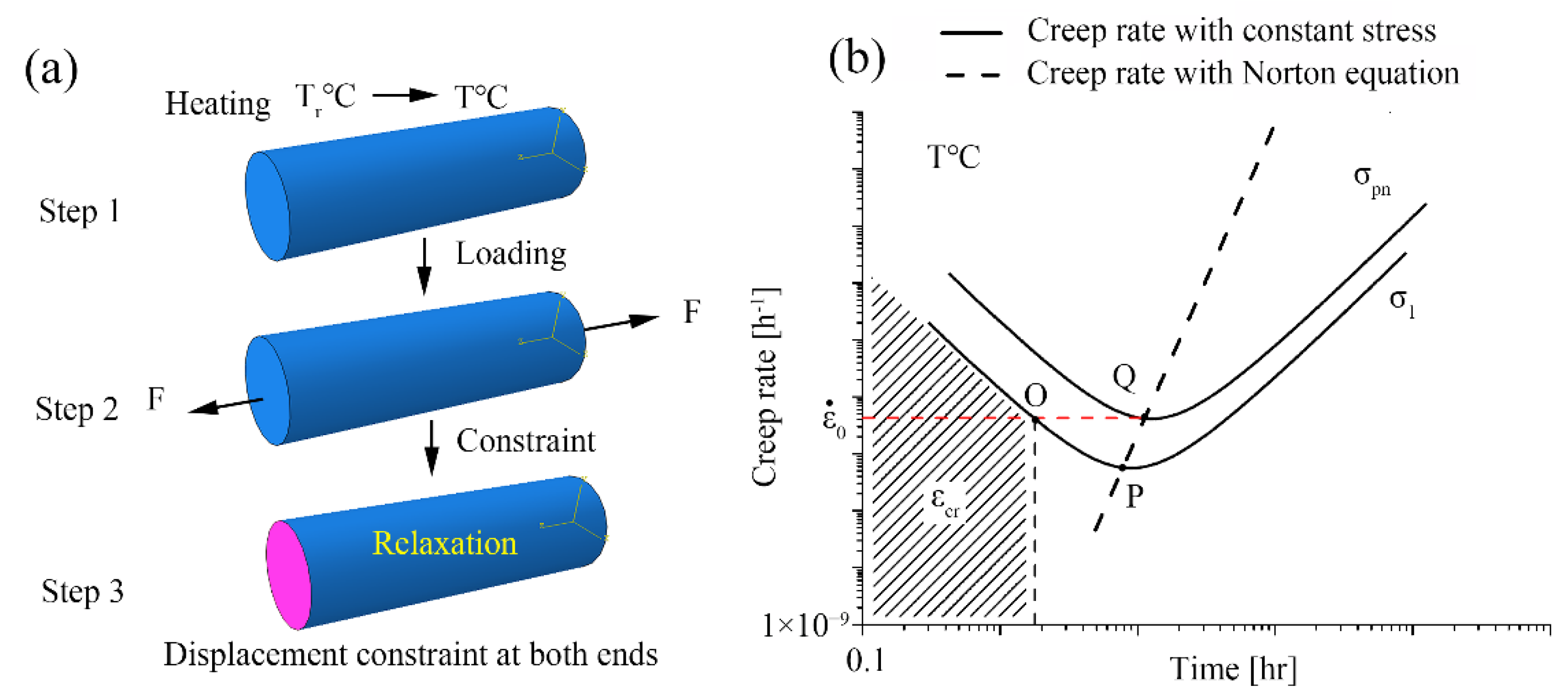
4.2. Stress Relief Analysis in Heat Treatment

A fully-coupled simulation was employed in stress relief analysis, which calculated the temperature field, elastic-plastic strain, and creep strain at the same time. The as-welded residual stress information from the mechanical analysis was preset initially by mapping residual stresses and plastic strains onto the same axisymmetric model in nodes with the Predefined-Field module in ABAQUS. The selected element type is CAX4RT (A 4-node thermally coupled axisymmetric quadrilateral element with bilinear displacement and temperature, reduced integration and hourglass control). Creep strain was considered during holding time when the temperature remained, reducing the calculating time and space. The sink temperature was set corresponding to the preset temperature curve in the furnace with subroutine FILM in ABAQUS. Heat convection and radiation were also set as the thermal boundary condition. Rigid body movement was restricted with an angular point constrained.
Creep equations estimating creep behavior were described and obtained in Section 2. The creep equation was employed in the form of strain-hardening with the Material-Property module in ABAQUS. The time index for Norton equation was zero, which neglected the strain hardening during creep strain accumulation. The simulation routine called variables including creep strains and stresses from each node to calculate the increment of creep strains with creep equations during every time increment in simulation, which contributed to strain coordination.

4.3. Numerical Experiments

Table 4 listed the experimental scheme for the study. Norton and Norton-Bailey equations were employed in simulation at 500, 560, 600, and 630 °C for comparison. A welded specimen was manufactured and heat-treated at 560 °C. As-welded and PWHT residual stresses were measured with the hole-drilling method in order to validate the simulation model.

5. Experimental Validation

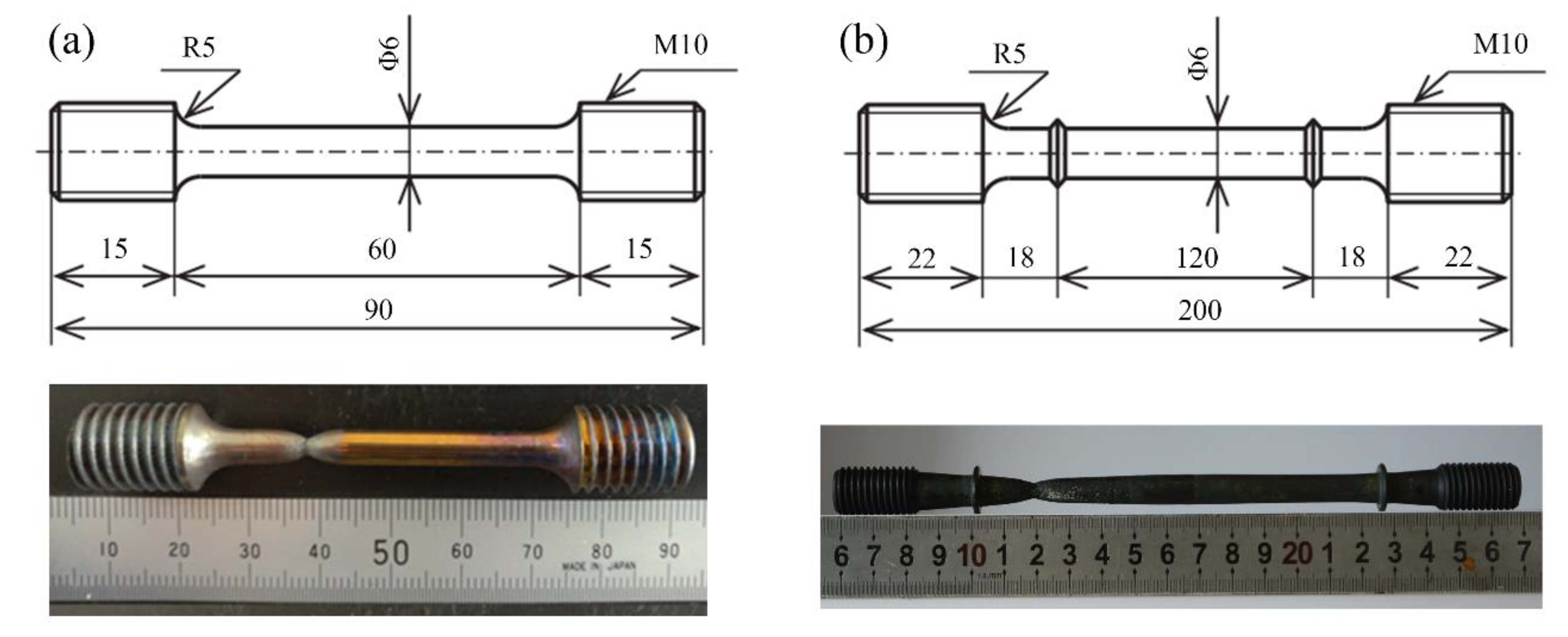
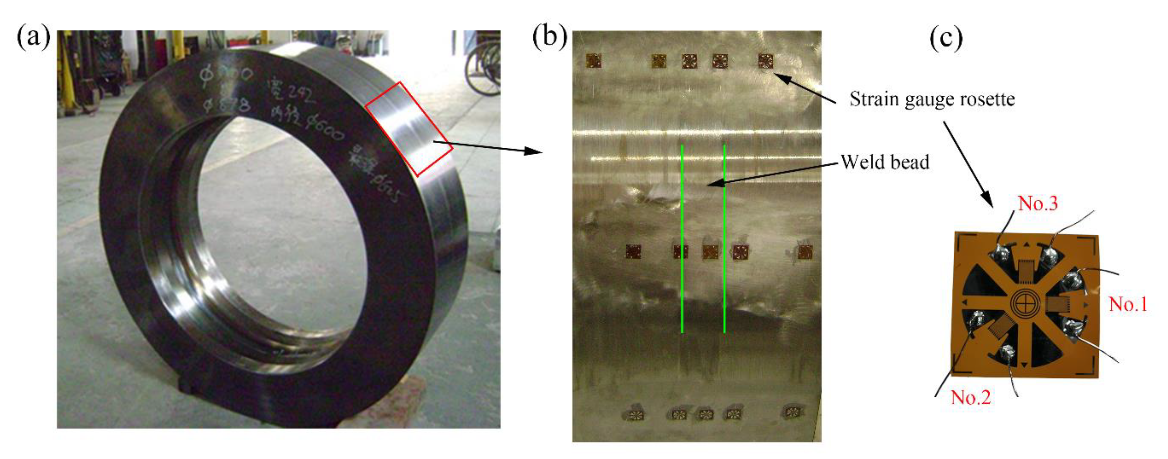
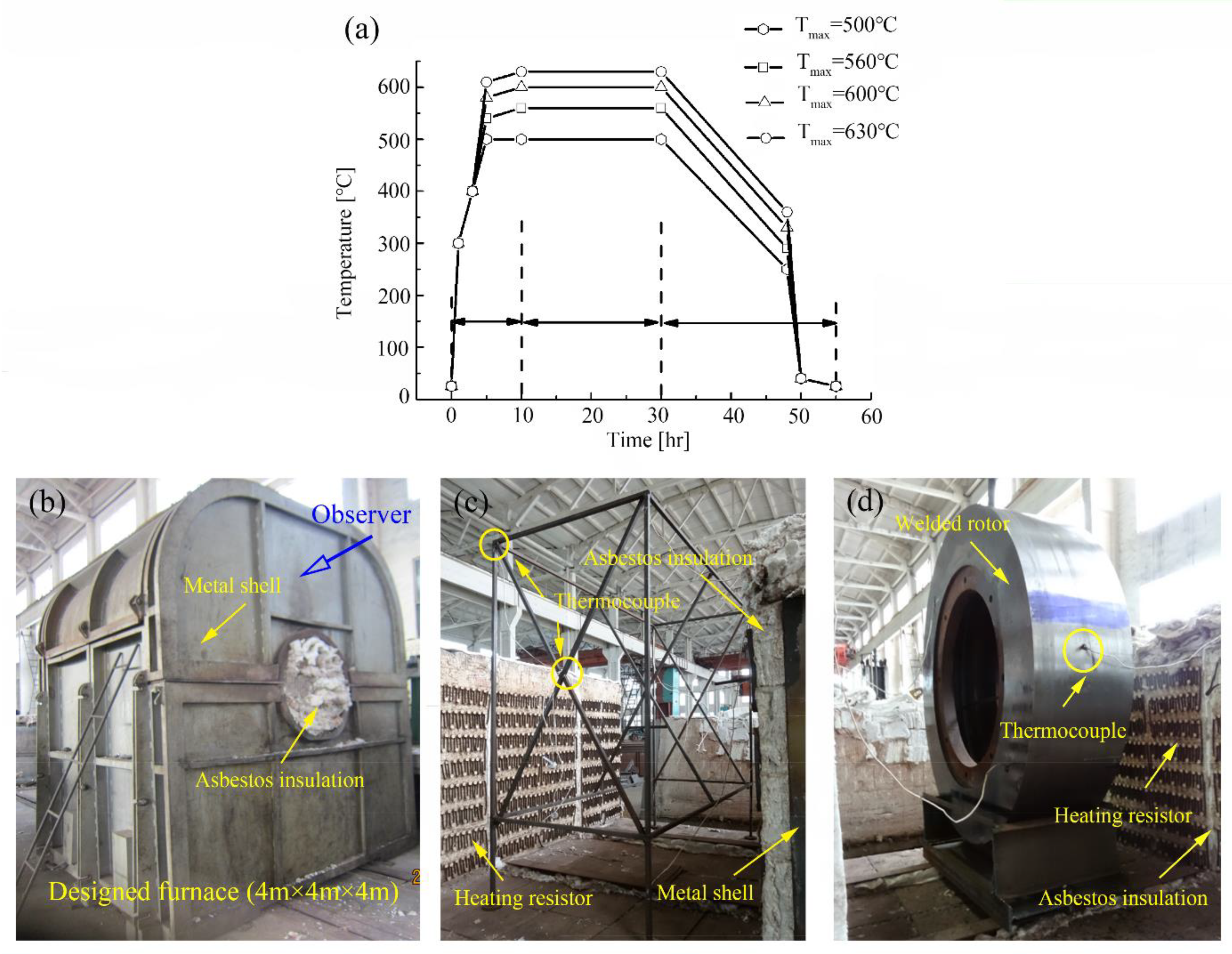
5.1. Welded Specimen and Heat Treatment

Two ring-shaped members were welded with submerged arc welding to manufacture the rotor, of which the outer diameter and inner diameter were approximately 900 and 600 mm respectively, as shown in Figure 7a. The axial length of the rotor was approximately 240 mm and the cap weld was approximately 30 mm in width. The base metal was 25Cr2Ni2MoV steel and the weld metal was similar to the base metal in terms of chemical compositions. Subsequently, the same thermal and elastic-plastic properties were employed in the numerical simulation, as shown in Section 2. The geometry of the welded rotor was determined according to one product from the Shanghai Turbine Plant. The voltage and electricity of submerged arc welding were 25–35 V and 450–500 A, respectively. The rotor was machined to eliminate the weld cap immediately after welding so as to facilitate stress measurement. The welded rotor was treated at 560 °C for 20 h in a furnace post welding. The temperature setting in the furnace is shown in Figure 8a. The temperature and operating time were determined based on the balance of stress relief and mechanical property improvement while considering time efficiency. The temperature should be 100–200 °C below the transformation temperature from ferrite to austenite [21], which is approximately 510–610 °C for 25Cr2Ni2MoV steel. The holding time is decided by the operability under the engineer condition, taking into account the evolution of the toughness and microstructure. Finally, a heat treatment at 560 °C for 20 h was employed in the investigation.
A furnace was employed, as shown in Figure 8b. It consists of seven assembled metal structures with asbestos insulations attached on the inner surface to block heat loss. Dimensions of the furnace are 4 m in length, 4 m in width, and 4 m in height. Heating resistors were attached on asbestos insulations on vertical walls to produce heat. The temperature was monitored with 12 thermocouples in the furnace and controlled with feedback regulation. As shown in Figure 8a, time for the heating up process was 10 h and holding time was 20 h. In the cooling process, the temperature evolved from 560 °C to room temperature in 25 h.

5.2. Residual Stress Measurement with HDM

The hole-drilling method (HDM) was employed to measure residual stresses on outer and inner cylindrical surfaces post weld and heat treatment. Stresses obtained with HDM are the average stress within the drilled hole [22], which is assumed to be in the plane stress condition. In this study, the depth and diameter of the hole were 2 and 1.5 mm, respectively. The diameter is the appropriate size, which was minimized such that the drill would not break and to reflect the residual stress accurately. The principal stresses and their direction can be expressed as follows:
σ m a x = ε 1 + ε 3 4 A r + 1 4 B r ( ε 3 ε 1 ) 2 + ( ε 3 + ε 1 2 ε 2 ) 2
σ m i n = ε 1 + ε 3 4 A r 1 4 B r ( ε 3 ε 1 ) 2 + ( ε 3 + ε 1 2 ε 2 ) 2
tan 2 γ = ε 1 2 ε 2 + ε 3 ε 1 ε 3
where σ m a x and σ m i n are principal stresses; ε 1 , ε 2 , and ε 3 present the relieved strain at each corresponding gauge; γ is the angle from σ m a x to gauge no. 1. The stress relief coefficients A r and B r are 0.07255 and 0.1514, respectively. Meanwhile, the additional strain ε m caused by machining is −39 μ ε .
The strain gauge rosette used in the measurement was denoted TJ120-1.5-Φ1.5, a size of which was 10 mm × 10 mm as shown in Figure 7c. The strain gauge rosette was composed of three gauges in different directions on the circumference. The size of each gauge was 1.5 mm × 1.5 mm and the resistance was 120 Ω. The strain gauge rosette could be applied to HDM with a diameter of the hole being 1.5 mm. The sensitivity coefficient of each resistance strain gauge was 2.07 ± 0.01, which indicated that the maximum error was about 0.97%. The alcohol solution containing 4% nitric acid (volume fraction) was used to corrode the weld in order to locate the strain gauge rosette accurately. The weld seam and heat affected zone can be distinguished clearly on the corroded weld. The ruler and scriber were employed to help determine the location and direction of the strain gauge rosette. The strain gauge rosette was glued to the weld with gauge no. 1 along the axial direction and gauge no. 3 along the circumferential direction. The strain gauge rosettes were located at 0, 13, 15, and 65 mm away from the weld center line to visualize stress distribution, similar to those shown in Figure 6b. In order to reduce random error, the residual stress of each test point was measured three times and averaged. The measured results have also been presented together with the simulation results. The measured data indicated that the error was within 10 MPa, which resulted from the deviation of sensitivity coefficient, patch position, and direction of strain gauge rosette. Furthermore, a deviation of weld width could result in a deviation of patch position relative to the heated affected zone, although the weld width fluctuated to 30 ± 0.1 mm.

6. Results and Discussion

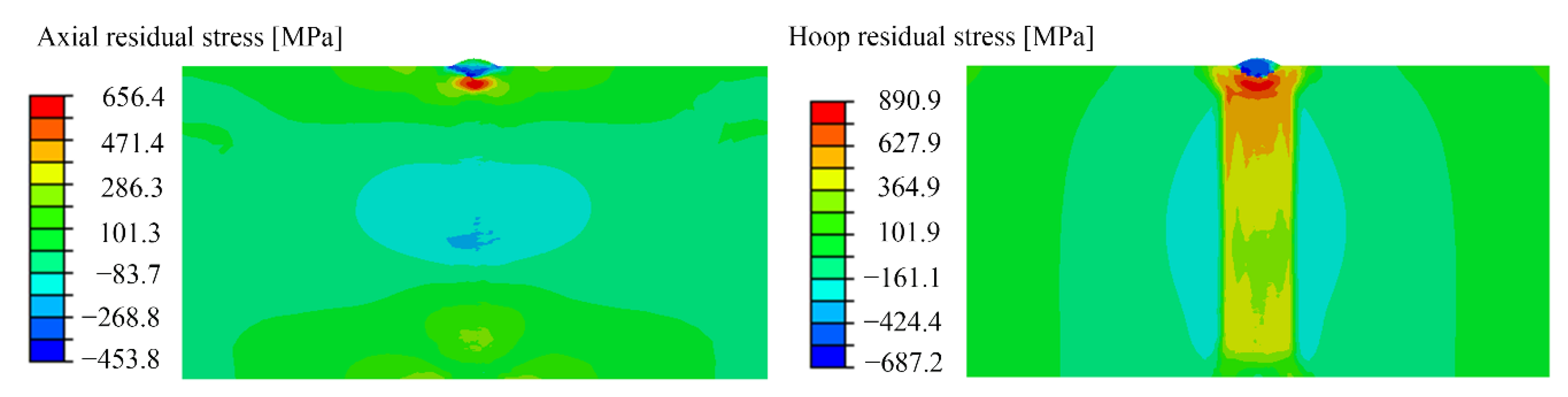
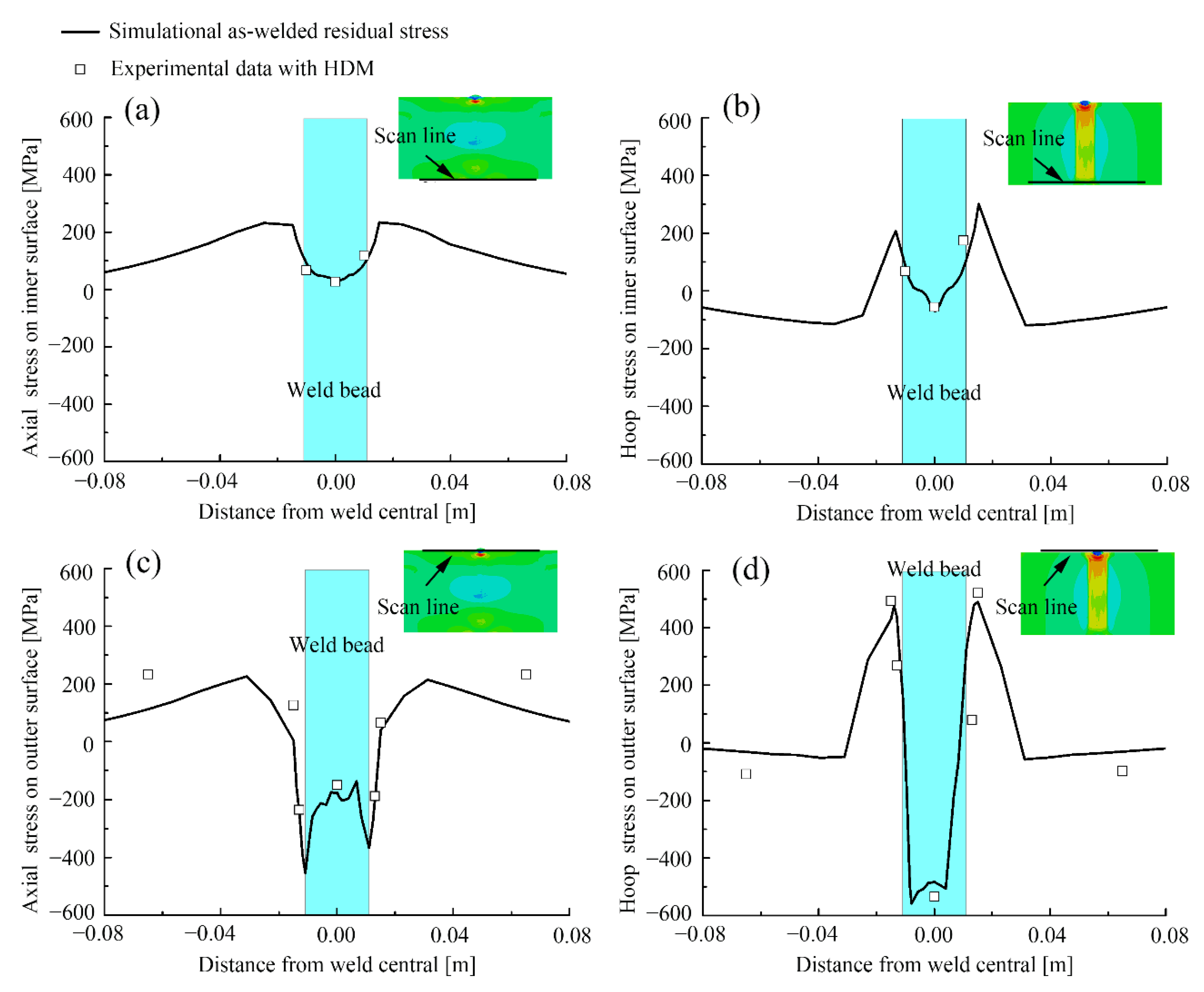
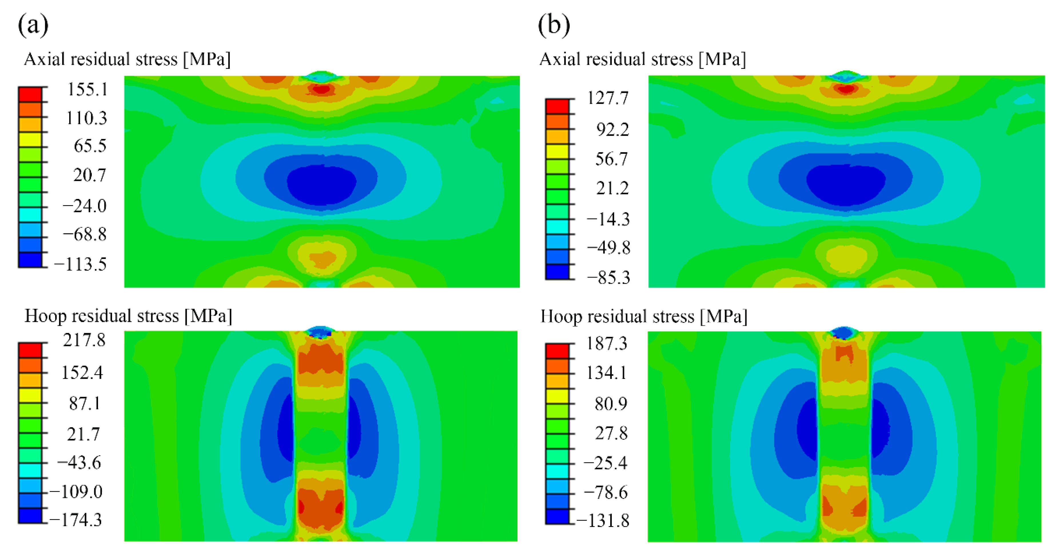
6.1. As-Welded Residual Stress

Contour plots of axial stress and hoop stress on the axisymmetric surface are presented in Figure 9. Axial stress and hoop stress in the cap weld are compressive, which may result from martensitic transformation at low temperatures [23]. The compressive stresses are balanced by tensile stress under the cap in the weld. It is also noted that the central region of the axisymmetric surface is characterized by compressive axial stresses and tensile hoop stresses. The compressive axial stresses are balanced by the stresses in the other part. Meanwhile, tensile hoop stresses in the weld bead are balanced by compressive stresses alongside the weld. It also indicates that axial stress and hoop stress on the inner surface in the weld are compressive and tensile, respectively. As shown in Figure 9, the hoop residual stress in the weld bead is extremely high, being approximately 891 MPa. However, the yield stress of 25Cr2Ni2MoV steel is approximately 780 MPa at room temperature, as shown in Figure 3c. It can be explained that the linear isotropic hardening rule was taken into consideration in the investigation.
Comparing simulation results with experimental data, residual stress distribution from the simulation is also plotted along experimental scan lines in Figure 10. The stress distribution confirms general trends presented in Figure 9. It is also noted that simulation results are validated with experimental data in Figure 10. Some discrepancies come out between simulation results and experimental data, which may result from experimental measurement errors and the axisymmetric model [24,25]. The axisymmetric model neglects restriction from a colder region in front of the arc and after the arc.

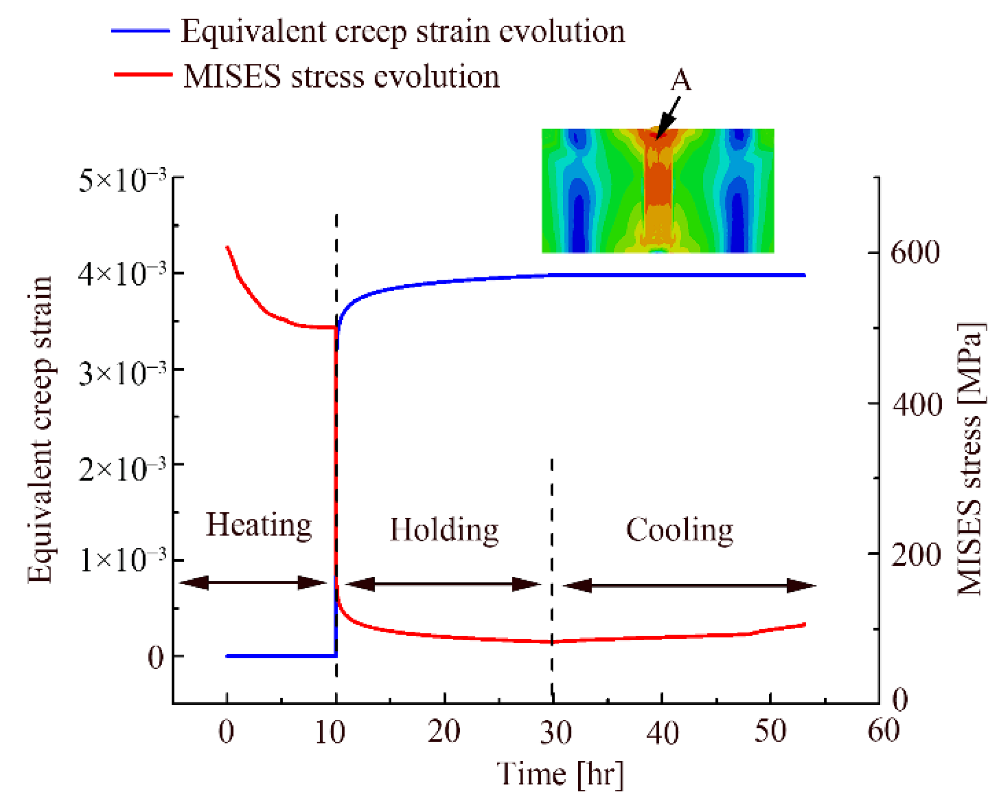
6.2. Stress Relaxation during PWHT

Figure 11 presents contour plots of the PWHT axial and hoop residual stress on axisymmetric faces, including the PWHT residual stress with Norton equation (Figure 11a) and Norton-Bailey equation (Figure 11b). The PWHT residual stress distribution is similar to the as-welded residual stress (Figure 9) and is numerically close to a stress-free state. As shown in Figure 9, the as-welded residual stress is concentrated in the weld and heat affected zone, where stress relaxation is induced during heat treatment. Compared with the as-welded residual stress, stress relaxation reduced the tensile hoop residual stress in the weld and tensile hoop residual stress appeared in the vicinity of the outer surface of the base metal owing to a mechanical equilibrium, as shown in Figure 11. The axial residual stress distribution trend remained almost the same as the as-welded residual stress. The axial stress in the weld on the inner surface evolved from tensile stress to compressive stress after PWHT, implying the strain coordination in PWHT.
Comparing simulation results and experimental data, residual stress distributions from the simulation with Norton equation and Norton-Bailey equation are plotted along lines on the outer and inner surfaces in Figure 12. Simulation results with Norton-Bailey equation are more accurate, which is validated by experimental data.
Based on the numerical simulation, an effect of temperature on eliminating residual stress during heat treatment can be analyzed. Considering that the von-Mises stress is a yield criteria and the main driving force for creep, as shown in Equation (18) corresponding to Norton-Bailey creep model.
ε ˙ i j = 3 2 A σ ¯ n 1 s i j t m
where ε ˙ i j is the deviator strain rate, σ ¯ is the von-Mises stress (MISES), and s i j is the deviator stress. Figure 13 presents the PWHT residual stress at different temperatures in the form of MISES along the outer line. It indicates that residual stresses simulated with Norton equation is higher in number than that simulated with Norton-Bailey equation. The difference between residual stresses simulated with Norton equation and Norton-Bailey equation decreases as the heat treatment temperature increases. The residual stresses in weld bead are almost the same at 600 and 630 °C. Meanwhile, it is obvious that more stress is eliminated when the heat treatment temperature is higher. All of the abovementioned phenomena are also presented with analytical solutions, as shown in Figure 5.
Table 5 lists the calculating time and space employed in simulations with Norton equation and Norton-Bailey equation. It indicates that simulations with Norton equation have a great superiority in both computing time and space. It is predicted that the superiority will be more evident in large-scaled and complex structures. Considering the discussion above, Norton-Bailey equation should be employed at low temperatures to ensure the calculation accuracy. Meanwhile, Norton equation should be used at high temperatures to reduce the calculation complexity. It seems that Norton equation should be employed at temperatures higher than 600 °C in this study. For other cases, it is important to find the demarcation temperature conveniently, which can be obtained easily with the one-dimensional analytical model, as shown in Section 3.

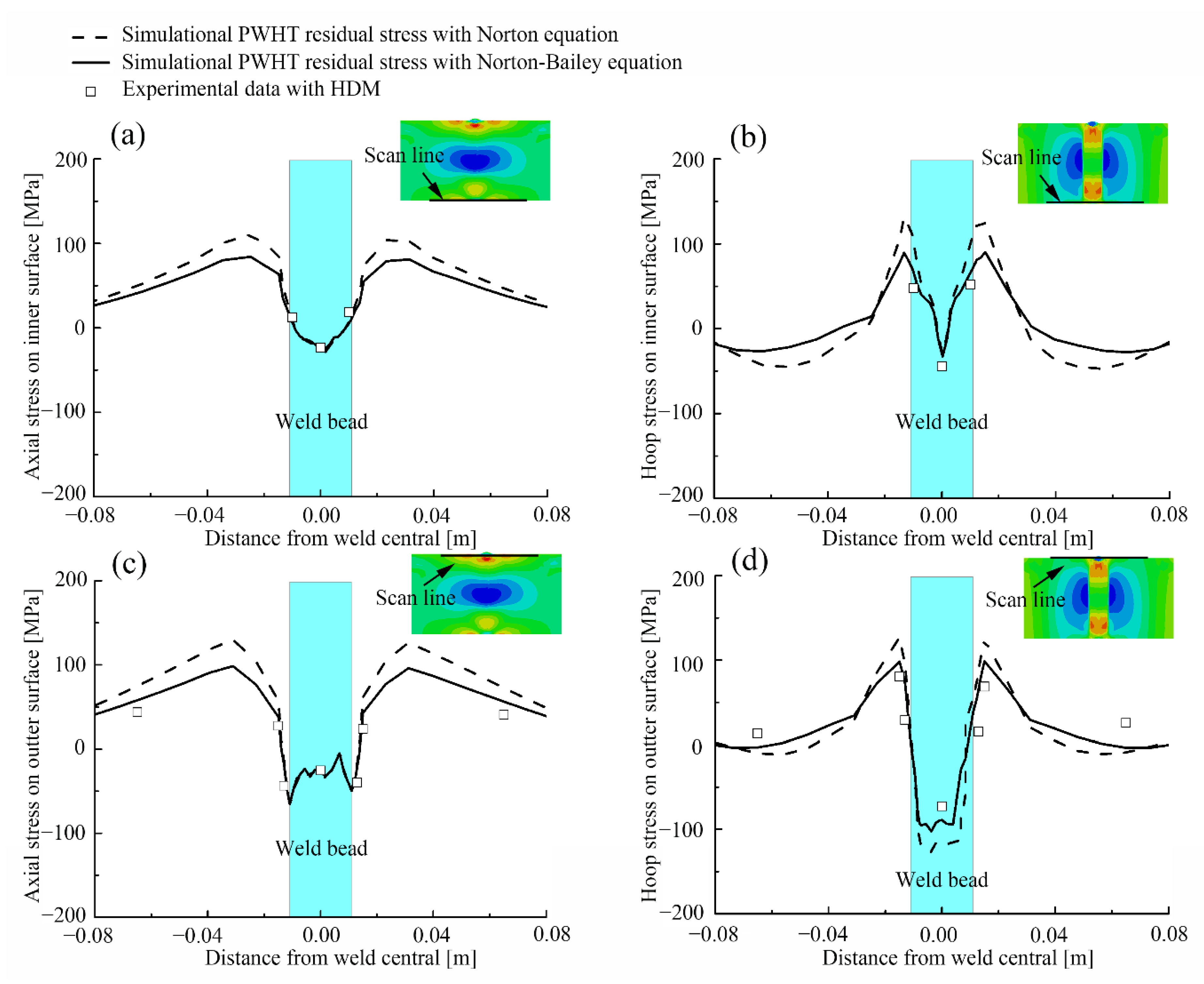
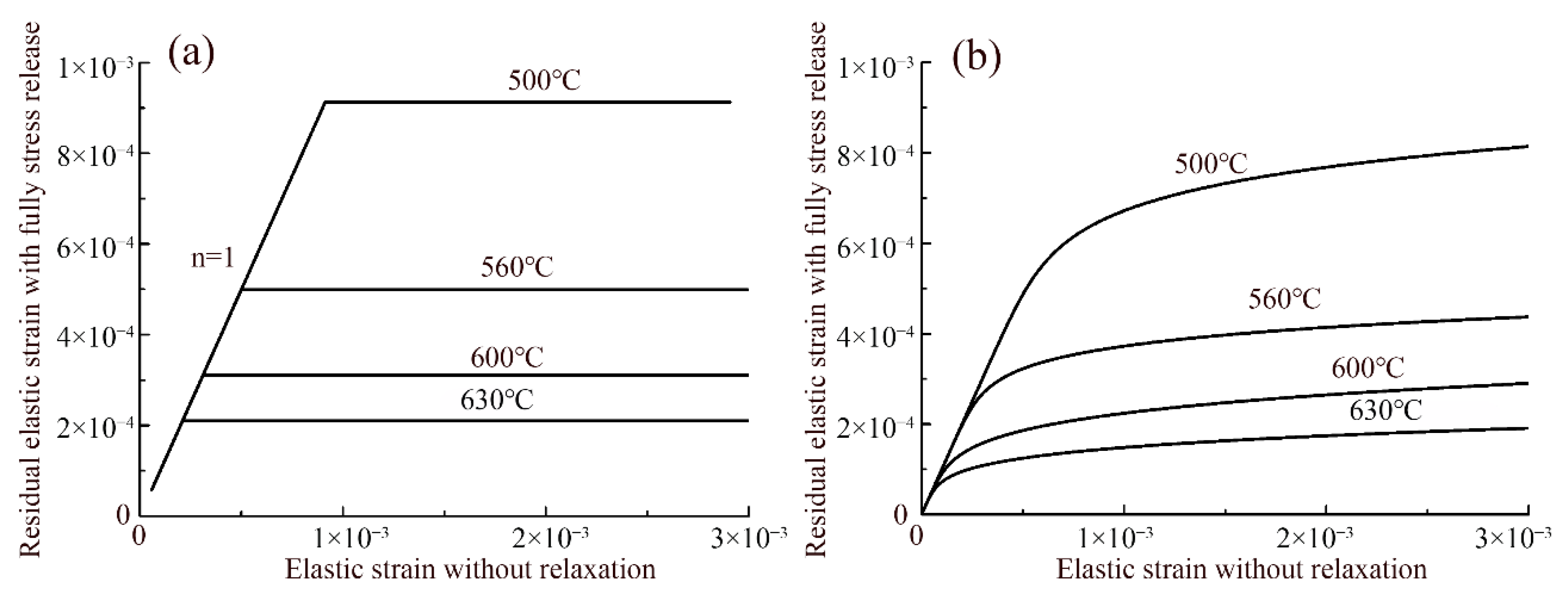
6.3. Comparison between Analytical Solutions and Simulation Results

The analytical model was assessed with numerical simulation and experimental results. The distribution on the outer cylindrical surface was predicted with the analytical model, as shown in Figure 13 with an imaginary line. Figure 13 indicates that stresses predicted with the analytical model in the weld bead and adjacent areas are lower than those simulated results with Norton equation or Norton-Bailey equation, separately. While stresses predicted with the analytical model in the base metal are higher than those simulated results. It can be explained that the stresses are released out of proportion in a three-dimensional simulation, which leads to compatible deformation. The deformation coordination contributes to that a higher initial stress corresponds to a higher residual stress. Figure 14 presents the relationship between initial stresses and residual stresses at different temperatures, which are all divided by Young’s modulus to obtain the elastic strain. As shown in Figure 14a, the elastic strains for creep initiation are smaller at a higher temperature, which will also lead to deformation coordination during the process of heating up. Considering the discussion above, the results predicted with the analytical model will introduce deviation owing to neglecting deformation coordination. It is necessary to obtain accurate results with numerical simulation to take more relevant factors into account. However, the analytical model can help investigate the approximate temperature range for heat treatment, taking σ p n as the largest PWHT residual stress, as shown in Figure 5 and Figure 13.

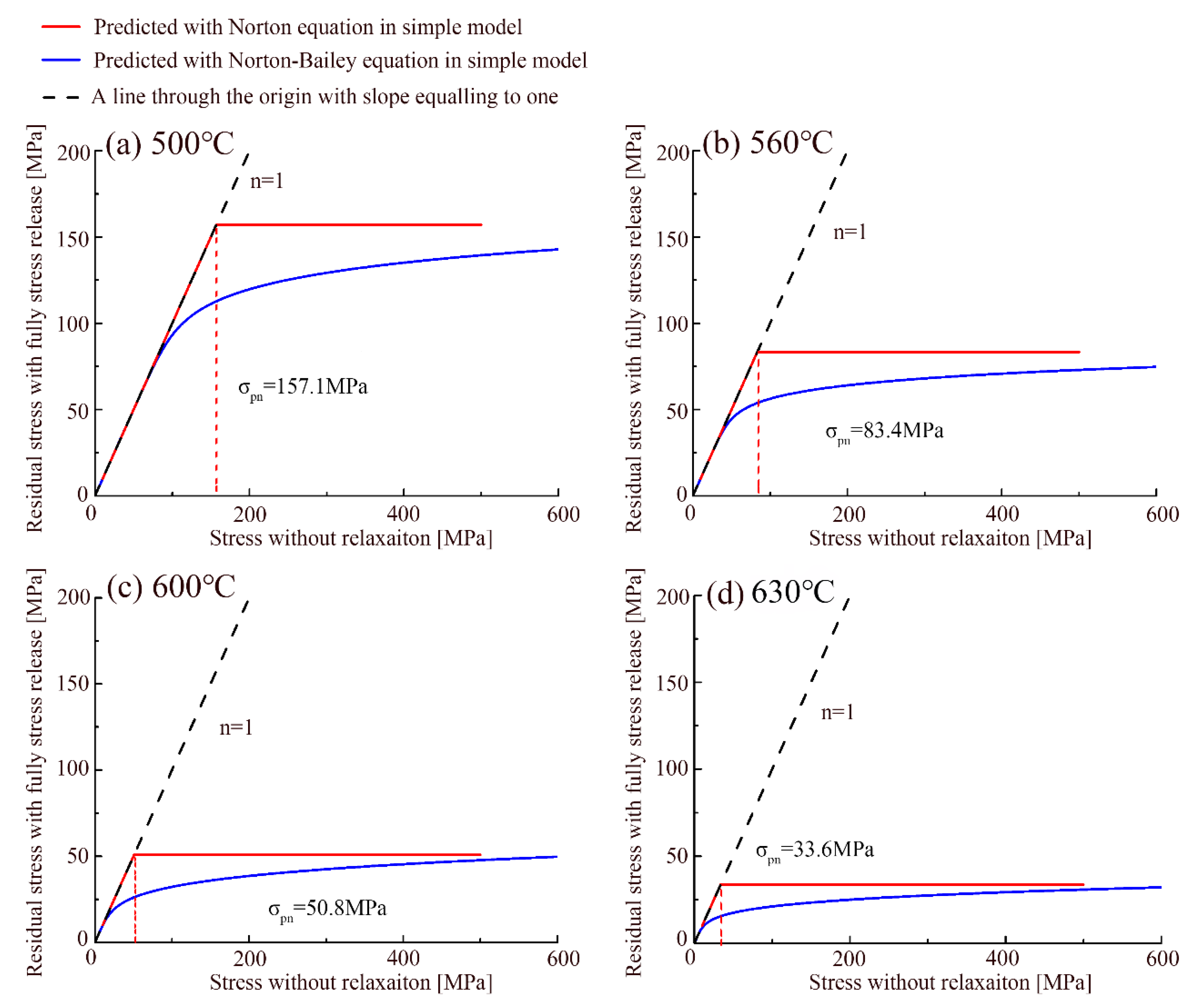
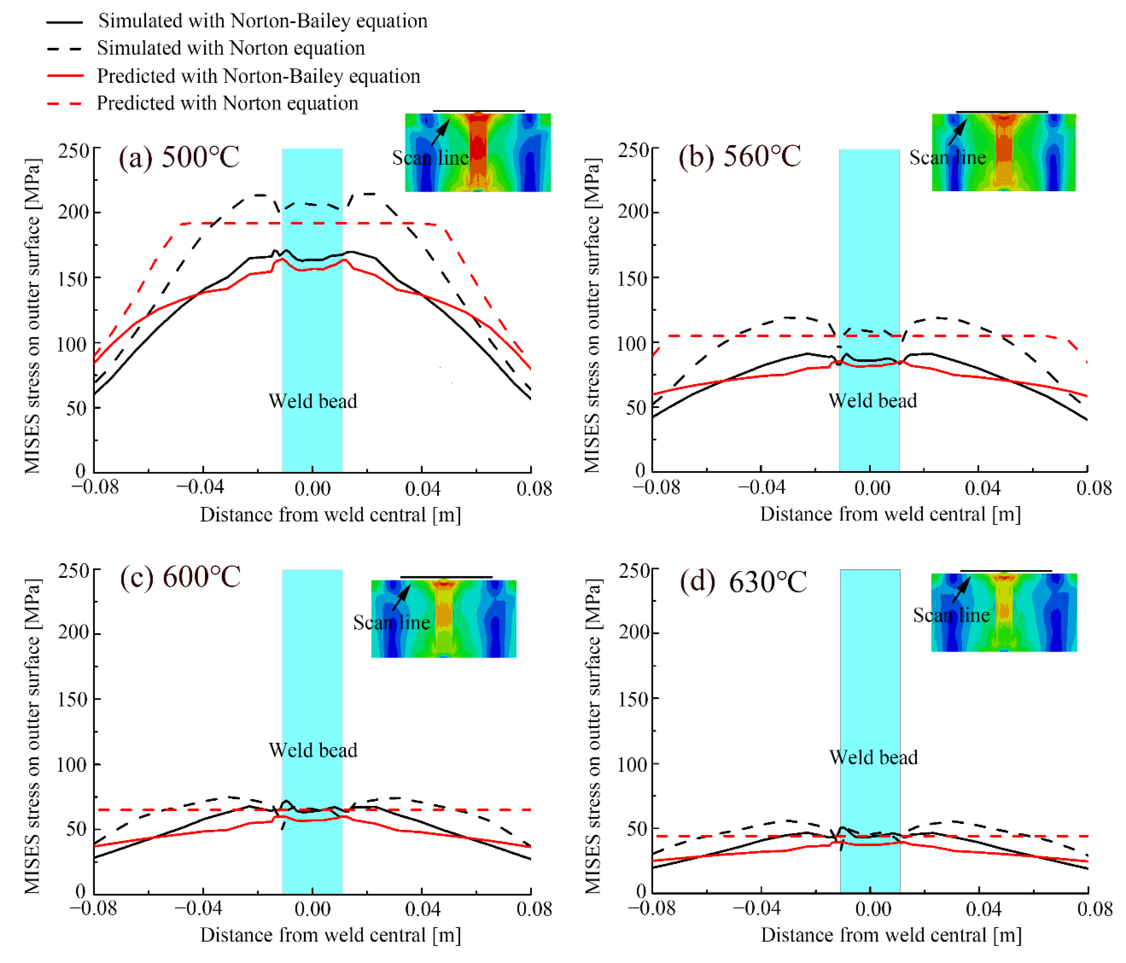
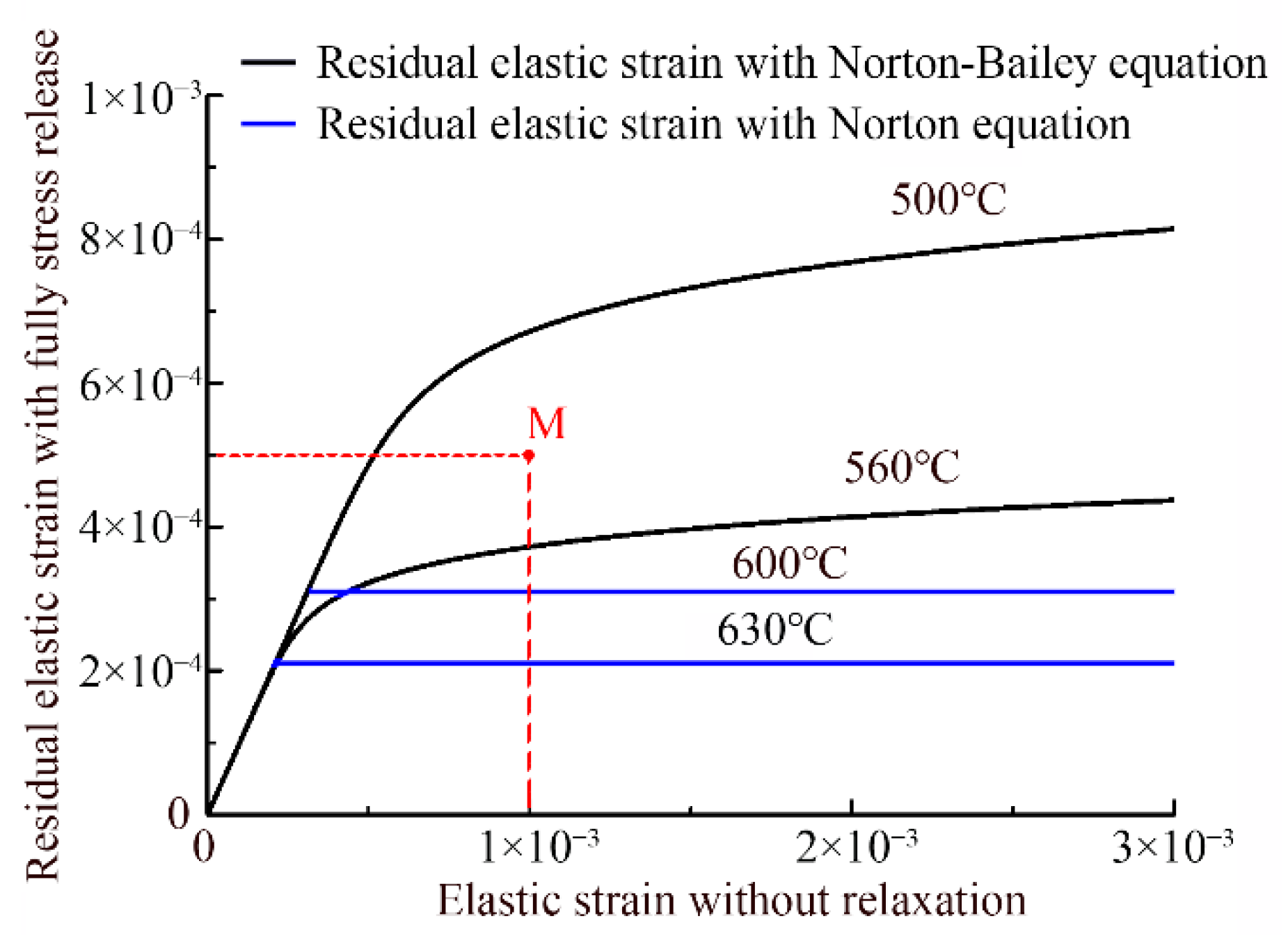
6.4. Effect of PWHT Temperature on Stress Relaxation and Creep Equation Selection

As shown in Figure 13, deviation between residual stresses predicted with Norton equation and Norton-Bailey equation decreases as temperature increases. With the temperature increasing, atomic diffusion plays a greater role in creeping rather than stress, which contributes to a lower PWHT residual stress and decreases the deviation. Figure 13 indicates that the deviation is very small at 600 and 630 °C, which is also present in Figure 5. In order to help select creep equation and investigate the approximate temperature range for heat treatment, Figure 14 can be plotted in a graph as shown in Figure 15. The lines corresponding to Norton and Norton-Bailey equation at 600 and 630 °C are close to each other. Therefore, the lines corresponding to Norton-Bailey equation have been neglected. Given that the as-welded residual stress and the expected PWHT residual stress are known as the Node M, as shown in Figure 15, it is obvious that the heat treatment temperature should be between 500 and 560 °C. Meanwhile, Norton-Bailey equation should be employed in the simulation to obtain PWHT residual stresses in a three-dimensional model.
Figure 16 obtains the evolution of MISES stress and creep strain at Node A during the process of heat treatment at 560 °C. It indicates that creep strain was accumulated and stress was released in a short time. Taking Figure 13 and Figure 16 into consideration, it indicates that the heat treatment temperature is more effective than the holding time. Therefore, the holding time for heat treatment should be determined based on the requirement of mechanical properties and evolution of microstructures during heat treatment.

7. Conclusions

The one-dimensional analytical model was promoted to investigate different effects of Norton and Norton-Bailey creep constitutive equation on stress relief during heat treatment in a ferritic welded rotor. The analytical solutions were compared with simulation results, which were validated with experimental measurements. The following conclusions can be drawn:
(1)
Norton equation should be employed in the stress relief simulation instead of Norton-Bailey equation to reduce the calculation complexity exceeding 600 °C.
(2)
The PWHT residual stress calculated with Norton equation is higher than that with Norton-Bailey equation.
(3)
With the PWHT temperature increasing, the deviation between Norton equation and Norton-Bailey equation decreases.
(4)
The one-dimensional analytical model was promoted to help select a creep constitutive equation and predict an appropriate range of heat treatment temperature, along with neglecting the impact of structural constraint and deformation compatibility.
(5)
Deformation coordination plays an important role in stress relaxation in heat treatment.

Author Contributions

Conceptualization, M.H., K.L., and Z.C.; methodology, M.H. and S.L.; resources, Z.C. and J.P.; writing—original draft preparation, M.H.; writing—review and editing, K.L. and Z.C.; project administration, K.L., Z.C., and J.P. All authors have read and agreed to the published version of the manuscript.

Funding

The research work presented in this paper has been supported by the Shanghai Turbine Plant and National Natural Science Foundation of China (No. 51775300 and No. 51901113). They are profoundly appreciated. The authors also express their gratitude to Wangteng Cai (Fox Valley Lutheran High School) for help in the writing of the article.

Conflicts of Interest

The authors declare no conflict of interest.

References

  1. Li, Y.; Li, K.; Cai, Z.; Pan, J.; Liu, X.; Wang, P. Alloy design of welding filler metal for 9Cr/2.25Cr dissimilar welded joint and mechanical properties investigation. Weld. World 2018, 62, 1137–1151. [Google Scholar] [CrossRef]
  2. Webster, G.; Ezeilo, A. Residual stress distributions and their influence on fatigue lifetimes. Int. J. Fatigue 2001, 23, 375–383. [Google Scholar] [CrossRef]
  3. Marshall, D.B.; Lawn, B.R. Residual stress effects in sharp contact cracking. J. Mater. Sci. 1979, 14, 2001–2012. [Google Scholar] [CrossRef]
  4. Cheng, X. Residual stress modification by post-weld treatment and its beneficial effect on fatigue strength of welded structures. Int. J. Fatigue 2003, 25, 1259–1269. [Google Scholar] [CrossRef]
  5. Bussu, G.; Irving, P.E. The role of residual stress and heat affected zone properties on fatigue crack propagation in friction stir welded 2024-T351 aluminum joints. Int. J. Fatigue 2003, 25, 77–88. [Google Scholar] [CrossRef]
  6. Turski, M.; Bouchard, P.J.; Steuwer, A.; Withers, P.J. Residual stress driven creep cracking in AISI Type 316 stainless steel. Acta Mater. 2008, 56, 3598–3612. [Google Scholar] [CrossRef]
  7. Francis, J.; Mazur, W.; Bhadeshia, H.K.D.H. Review Type IV cracking in ferritic power plant steels. Mater. Sci. Technol. 2006, 22, 1387–1395. [Google Scholar] [CrossRef]
  8. Dong, P.; Song, S.; Zhang, J. Analysis of residual stress relief mechanisms in post-weld heat treatment. Int. J. Press. Vessel. Pip. 2014, 122, 6–14. [Google Scholar] [CrossRef]
  9. Wang, J.; Lu, H.; Murakawa, H. Mechanical behavior in local post weld heat treatment (report i): Visco-elastic-plastic fem analysis of local pwht (mechanics, strength & structure design). Trans. JWRI 1998, 27, 83–88. [Google Scholar]
  10. Ueda, Y.; Fukuda, K. Analysis of welding stress relieving by annealing based on finite element method. Trans. JWRI 1975, 4, 39–45. [Google Scholar]
  11. Yanagida, N.; Ogawa, K.; Saito, K.; Kingston, E. Study on Residual-Stress Redistributions During the Process of Manufacture of a Vessel Penetration Set-On Joint. In Proceedings of the ASME 2009 Pressure Vessels and Piping Conference, Prague, Czech Republic, 26–30 July 2009. [Google Scholar]
  12. Ogawa, K.; Okuda, Y.; Saito, T.; Hayashi, T.; Sumiya, R. Welding residual stress analysis using axisymmetric modeling for shroud support structure. In Proceedings of the ASME 2008 Pressure Vessels and Piping Conference, Chicago, IL, USA, 27–31 July 2008. [Google Scholar]
  13. Udagawa, M.; Katsuyama, J.; Onizawa, K. Effects of residual stress by weld overlay cladding and PWHT on the structural integrity of RPV during PTS. In Proceedings of the ASME 2007 Pressure Vessels and Piping Conference, San Antonio, TX, USA, 22–26 July 2007. [Google Scholar]
  14. Takazawa, H.; Yanagida, N. Effect of creep constitutive equation on simulated stress mitigation behavior of alloy steel pipe during post-weld heat treatment. Int. J. Press. Vessel. Pip. 2014, 117, 42–48. [Google Scholar] [CrossRef]
  15. Creep-Resistant Steel; Abe, F.; Torsten-Ulf, K.; Ramaswamy, V. (Eds.) Elsevier: Amsterdam, The Netherlands, 2008; pp. 10–11. [Google Scholar]
  16. Li, C.; Han, L.; Yan, G.; Liu, Q.; Luo, X.; Gu, J. Time-dependent temper embrittlement of reactor pressure vessel steel: Correlation between microstructural evolution and mechanical properties during tempering at 650 °C. J. Nucl. Mater. 2016, 480, 344–354. [Google Scholar] [CrossRef]
  17. Goldak, J.; Chakravarti, A.; Bibby, M. A new finite element model for welding heat sources. Met. Mater. Trans. A 1984, 15, 299–305. [Google Scholar] [CrossRef]
  18. Bai, X.; Zhang, H.; Wang, G. Improving prediction accuracy of thermal analysis for weld-based additive manufacturing by calibrating input parameters using IR imaging. Int. J. Adv. Manuf. Technol. 2013, 69, 1087–1095. [Google Scholar] [CrossRef]
  19. Hu, M.; Li, K.; Cai, Z.; Pan, J. A new weld material model used in welding analysis of narrow gap thick-walled welded rotor. J. Manuf. Process. 2018, 34, 614–624. [Google Scholar] [CrossRef]
  20. Yaghi, A.; Hyde, T.; Becker, A.; Sun, W.; Williams, J. Residual stress simulation in thin and thick-walled stainless steel pipe welds including pipe diameter effects. Int. J. Press. Vessel. Pip. 2006, 83, 864–874. [Google Scholar] [CrossRef]
  21. Metal Materials and Heat Treatment; Cui, Z.; Liu, H. (Eds.) Central South University Press: Changsha, China, 2010. [Google Scholar]
  22. Vangi, D. Data Management for the Evaluation of Residual Stresses by the Incremental Hole-Drilling Method. J. Eng. Mater. Technol. 1994, 116, 561–566. [Google Scholar] [CrossRef]
  23. Neubert, S.; Pittner, A.; Rethmeier, M. Influence of non-uniform martensitic transformation on residual stresses and distortion of GMA-welding. J. Constr. Steel Res. 2017, 128, 193–200. [Google Scholar] [CrossRef]
  24. Murthy, Y.; Rao, G.; Iyer, P. Numerical simulation of welding and quenching processes using transient thermal and thermo-elasto-plastic formulations. Comput. Struct. 1996, 60, 131–154. [Google Scholar] [CrossRef]
  25. Dike, J.; Cadden, C.; Corderman, R.; Schultz, C.; McAninch, M. Finite element modeling of multipass GMA welds in steel plates. In Proceedings of the 4th International Conference on Trends in Welding Research, Gatlinburg, TN, USA, 5–8 June 1995; pp. 57–65. [Google Scholar]
Figure 1. Thermal properties of 25Cr2Ni2MoV steel.
Metals 10 00688 g001
Figure 2. (a) Shape and dimensions of tensile test specimens and (b) creep test specimens of 25Cr2Ni2MoV steel (unit: mm).
Metals 10 00688 g002
Figure 3. Mechanical properties of 25Cr2Ni2MoV steel versus temperature: (a) thermal strain; (b) Young’s modulus; (c) yield stress and (d) Poisson’s ratio.
Metals 10 00688 g003
Figure 4. (a) The one-dimensional analytical model and (b) diagram of the small creep rate at the end of creep strain accumulation in heat treatment corresponding to Norton equation and Norton-Bailey equation using the creep rate data from a creep rupture test with constant stress.
Metals 10 00688 g004
Figure 5. Relationship between initial stress and post heat-treatment stress with Norton and Norton-Bailey equation at different temperatures: (a) 500 °C; (b) 560 °C; (c) 600 °C and (d) 630 °C.
Metals 10 00688 g005
Figure 6. Simulation model of welded rotor (unit: mm): (a) Three-dimensional stereogram; (b) subdivision surface along the radial direction; (c) mapped meshing.
Metals 10 00688 g006
Figure 7. Welded rotor (a), deployment of strain gauge rosettes (b) and strain gauge rosette (c).
Metals 10 00688 g007
Figure 8. Temperature setting in furnace-based heat treatment for welded 25Cr2Ni2MoV steel rotor (a) and the furnace-based heat treatment: (b) The designed furnace (4 m × 4 m × 4 m); (c) interior of the designed furnace; (d) another welded rotor with a larger size in the furnace.
Metals 10 00688 g008
Figure 9. Contour plots of as-welded axial stress and hoop stress.
Metals 10 00688 g009
Figure 10. Comparison between simulation results and experimental data along the inner surface: (a) As-welded axial stress; (b) as-welded hoop stress; and along the outer surface: (c) As-welded axial stress; (d) as-welded hoop stress.
Metals 10 00688 g010
Figure 11. Contour plots of the post weld heat treatment (PWHT) axial stress and hoop stress: (a) With Norton equation and (b) with Norton-Bailey equation at 560 °C.
Metals 10 00688 g011
Figure 12. Comparison between PWHT simulation results and experimental data along the inner cylindrical surface: (a) PWHT axial stress; (b) PWHT hoop stress; and along the outer cylindrical surface: (c) PWHT axial stress; (d) PWHT hoop stress.
Metals 10 00688 g012
Figure 13. PWHT residual stress in the form of MISES along the outer line post heat treatment at different temperatures: (a) 500 °C; (b) 560 °C; (c) 600 °C and (d) 630 °C.
Metals 10 00688 g013
Figure 14. Relationship between initial stresses and residual stresses at different temperatures, which are all divided by Young’s modulus to obtain the elastic strain: (a) With Norton equation and (b) with Norton-Bailey equation.
Metals 10 00688 g014
Figure 15. Relationship between initial elastic strains and residual elastic strains at different temperatures, combining Norton equation and Norton-Bailey equation.
Metals 10 00688 g015
Figure 16. Evolution of MISES stress and creep strain at Node A during heat treatment at 560 °C.
Metals 10 00688 g016
Table 1. Chemical compositions of 25Cr2Ni2MoV steel (wt. %).
CMnSiNiMoCrVCoFe
0.250.650.070.731.102.400.30Bal.
Table 2. Conditions for creep tests.
Temperature [°C]Applied Stress [MPa]
500200, 240, 280,320
560140, 180, 220, 260
60090, 120, 150, 180
63050, 80,110, 140
Table 3. Material properties of 25Cr2Ni2MoV for the Norton and Norton-Bailey equation.
Temperature [°C]AnBum
500 2.31 × 10 27 9.57 7.14 × 10 19 6.61 0.67
560 4.03 × 10 21 7.69 1.96 × 10 13 4.56 0.52
600 1.22 × 10 17 6.62 6.57 × 10 9 2.32 0.48
630 3.86 × 10 15 5.75 4.26 × 10 8 1.98 0.42
Table 4. Experimental scheme for analysis.
Simulation and Experiment500 °C560 °C600 °C630 °C
Simulation with Norton
Simulation with Norton-Bailey
Experimental validation
Note: ○—conducted simulation, √—conducted measurement
Table 5. Calculating time and space employed in simulations.
PropertyCreep Equation500 °C560 °C600 °C630 °C
Calculating time [h]Norton equation2.322.352.412.37
Norton-Bailey equation4.214.144.294.25
Calculating space [Gb]Norton equation1.651.711.861.82
Norton-Bailey equation3.513.263.723.63

