Propagation and Depolarization of a Short Pulse of Light in Sea Water
by
Evgeniy E. Gorodnichev
1, 
Kirill A. Kondratiev
1,*,
Alexandr I. Kuzovlev
1 and
Dmitrii B. Rogozkin
1,2 1
Moscow Engineering Physics Institute, National Research Nuclear University MEPhI, Kashirskoe Shosse 31, Moscow 115409, Russia
2
Dukhov Research Institute of Automatics (VNIIA), Sushchevskaya Ulitza 22, Moscow 127055, Russia
*
Author to whom correspondence should be addressed.
J. Mar. Sci. Eng. 2020, 8(5), 371; https://doi.org/10.3390/jmse8050371
Submission received: 8 May 2020
/
Revised: 18 May 2020
/
Accepted: 20 May 2020
/
Published: 23 May 2020
(This article belongs to the Special Issue Light Fields in the Ocean from Natural and Artificial Sources)
Abstract
:We present the results of a theoretical study of underwater pulse propagation. The vector radiative transfer equation (VRTE) underlies our calculations of the main characteristics of the scattered light field in the pulse. Under the assumption of highly forward scattering in seawater, three separate equations for the basic modes are derived from the exact VRTE. These three equations are further solved both within the small-angle approximation and numerically. The equation for the intensity is analyzed for a power-law parametrization of the wings of the sea water phase function. The distribution of early arrival photons in the pulse, including the peak intensity, is calculated. Simple relations are also presented for the variance of the angular distribution of radiation, the effective duration of the signal and other parameters of the pulse. For linearly and circularly polarized pulses, the temporal profile of the degree of polarization is calculated for actual data on the scattering matrix elements. The degree of polarization is shown to be described by the self-similar dependence on some combination of the transport scattering coefficient, the temporal delay and the source-receiver distance. Our results are in agreement with experimental and Monte-Carlo simulation data. The conclusions of the paper offer a theoretical groundwork for application to underwater imaging, communication and remote sensing.
1. Introduction
Over several decades, studies on the propagation of light through highly forward scattering media has attracted great attention due to their potential applications to underwater wireless communication, imaging and remote sensing (see, e.g., [1,2,3,4,5,6,7,8,9,10,11,12,13,14]).
The significant attenuation and distortion of optical signals in sea water due to absorption and multiple scattering severely constrain the maximum operating range of laser-based systems. This places rather stringent requirements on a possibility to predict the optical channel characteristics, depending on actual sea water parameters. Of prime interest is information on the temporal stretching, spatial and angular broadening of a pulsed beam at the source-receiver distances up to several tens of the photon mean free paths in the medium.
Currently, numerical methods [3,4,5,6,9,11] (regarding earlier results see [15,16,17,18,19]) based primarily on Monte Carlo simulation are applied to computations of the light field distribution in sea water from non-stationary (pulsed, modulated) sources. These methods enable taking into account essentially all factors inherent in actual experimental conditions (the angular profile of the sea water phase function, the mutual source-receiver orientation, limited aperture and field-of-view of the receiver etc.). However, the results obtained in such a way, as a rule, are related to a particular set of parameters and can not be transfered directly to other cases. In this connection, there remains interest in finding analytical solutions to the radiative transfer equation that would be based on adequate approximations and satisfactory reproduce the light field distribution in sea water for actual values of the optical parameters.
In propagation of a short pulse through the highly forward scattering medium (, where is the average cosine of the single-scattering angle [2]) such as sea water, early arrival photons move along weakly curved trajectories and, as a consequence, exhibit relatively narrow angular distribution and small delay, ( is the photon path length, c is the speed of light in the medium, z is the source-receiver distance). These photons are the least depolarized. Just this component of light field is most important to underwater optical communication and imaging [2,3,6,11].
For the early arrival component of light field, the small-angle approximation can be applied to the non-stationary radiative transfer equation. Within this approximation, many studies of multiple scattering of a pulsed beam were carried out (see, e.g., [2,18,20,21,22,23,24,25,26,27,28,29,30,31,32,33]). Most of them [20,23,24,25,26,27,29,31,32,33] were based on the small-angle version of the Fokker-Planck approximation (or the diffusion approximation in the angular domain) for the collision integral in the radiative transfer equation. The results obtained within this exactly solvable model correlate only qualitatively with experimental data on the structure of a pulsed beam in sea water. This model based on the assumption that the mean square of the single-scattering angle exists within the small-angle phase function representation (i.e., that the phase function wings falls off rapidly [28,29,30]) can not describe adequately many of the pulsed beam characteristics (e.g., the distance dependence of the power attenuation, the temporal, angular and spatial broadening etc.). As analysis shows, the reason is that the phase function of sea water decreases rather slowly with increasing the scattering angle (roughly as [7,9,15,28]). This feature should be allowed for in solving the radiative transfer equation for sea water.
The aforesaid refers equally to the description of the polarization state of multiple-scattered light in sea water as depolarization results from scattering through relatively large angles [34,35,36]. The results derived within the small-angle diffusion approximation (see, e.g., [31,32,37,38,39]) can not be applied directly to sea water and other highly forward scattering media, such as aqueous suspension of polystyrene particles for which the depolarization of pulses has been studied both experimentally [40,41,42] and numerically using Monte Carlo [17,41] and DISORT [19] codes. Information on the degree of light polarization in the transmitted pulse is important for applying the polarization difference technique (see, e.g., [42,43]). When measuring the intensity difference between cross-polarized components, the pulse tail (i.e., the contribution from delaying photons) is cut off, which can be used in optical communication and imaging [42,43].
In what follows the distribution of light field and its polarization state in a -pulse propagating through sea water are studied. The basic mode approximation in the vector radiative transfer equation (VRTE) which we have applied previously to a stationary case (see, e.g., [35,36,44,45]) is generalized to calculating the temporal profiles of the intensity and the degree of polarization in the pulse. Our approach are based on a solution of the eigenvalue problem for the basic modes. The results of both analytical, within the small-angle approximation, and numerical calculations are presented. When performing the analytical calculations, we rely on the small-angle version of the Reynolds-McCormick phase function [46] and the Rayleigh approximation for the scattering matrix. Actual data on the sea water phase function [47,48] and the Voss-Fry scattering matrix [49] are used in our numerical calculations. The power-law parametrization is shown to be valid for the eigenvalues appearing in the expressions for the Laplace transform of the basic modes with respect to time. This enable expressing the distribution of light field in the pulse and the degree of polarization in a self-similar form. Our results are in agreement with data of experiment [7] and Monte Carlo simulations [17].
2. Theoretical Background
2.1. Vector Radiative Transfer Equation
Consider a pulsed beam of polarized light propagating in a scattering and absorbing medium. The medium is assumed to be a statistically isotropic disordered ensemble of scatterers. The intensity and the polarization state of scattered light are described by the Stokes column vector [50,51]
The Stokes parameters I, Q, U and V, and the components and of the electric field appearing in Equation (1) are defined in the system of unit vectors , , and . The unit vector =() is the direction of propagation of the transverse electromagnetic wave, the vector lies in the plane formed by the vectors and (the unit vector is directed along z-axis of the reference frame), the vector is perpendicular to this plane. The brackets denote statistical averaging.
The intrinsic properties of the medium is described by the scattering matrix where . For a macroscopically isotropic and symmetric medium, the scattering matrix has the block-diagonal form (see, e.g., [50,51]):
For the forward scattering (, ), the matrix is diagonal: and [51]. The matrix element appearing in matrix (2) is the scattering phase function normalized by the relation
Under multiple scattering conditions, it is convenient to go from the linear basis (see Equation (1)) to the circular basis [52], where the electric field is defined in the system of unit vectors as superposition of waves with right (+) and left (−) circular polarizations. For the circular basis, column vector [51,52]
is an analog of the Stokes vector (1). The vector obeys the non-stationary VRTE of the form [51,52]
where c is the speed of light in the medium, is the coefficient of total extinction, and are the coefficients of scattering and absorption, respectively. The phase matrix entering into Equation (5) is given by [51]
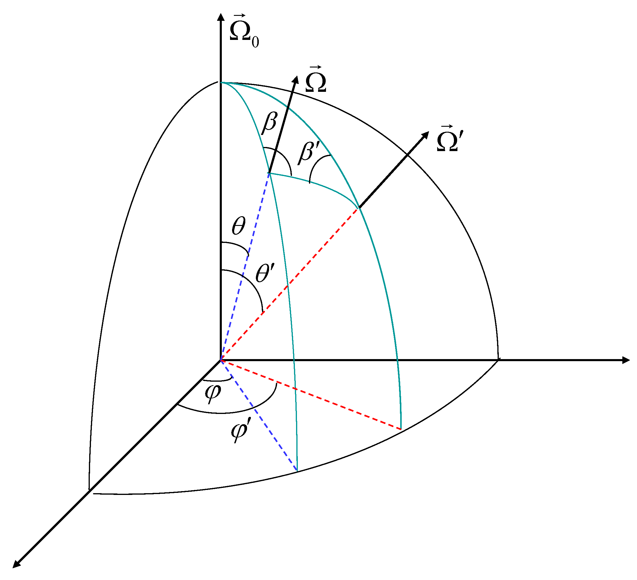
where , the angles and (see Figure 1) are defined by formulas
Functions and are obtained from Equation (7) by interchanging and .
The functions ( and ) and entering into Equation (6) are expressed in terms of the elements of the scattering matrix (2) by the relations
In the limiting case of weakly refractive particles (, where , d and n are the size and the relative refractive index of the particles, is the wavelength of light), all elements are expressed in terms of as follows [51]
Relations (10) correspond to the Rayleigh scattering matrix (see, e.g., [50,51]).
2.2. Basic Mode Approximation
In propagation of light through sea water and other media with weakly refractive large (the size d is larger than the wavelength ) inhomogeneities single scattering through small angles dominates. In this case the off-diagonal elements of the phase matrix appearing in Equations (5) and (6) turn out to be small as compared to the diagonal ones (see, e.g., [35,36,45]). In the first approximation we can neglect the off-diagonal elements. Then Equations (5) and (6) are reduced to three independent transfer equations [34,35,36,44,45,53]. These equations describe propagation of the individual modes I, and V appearing in Equation (4).
The specific intensity I is subject to the ordinary scalar transfer equation (see, e.g., [2,21])
Quantity W was named [44] by the basic mode of linear polarization. The transfer equation for W has the form
The separate equation for W was also derived in a different way, without resorting to the circular representation, in [53].
For a circularly polarized light ( in the source), the basic mode approximation is similar to that discussed above. When neglecting the off-diagonal elements, we arrive at the individual transfer equation for the basic mode V of circular polarization,
Equations (11)–(13) are valid for arbitrary initial polarization of light. In particular, for the elliptically polarized light, the initial values of the functions W and V entering into Equations (12) and (13) are equal to , where I and are the intensity and the degree of circular polarization of the source.
For a -pulsed unidirectional source emitting light along z-axis, the initial condition to Equation (11) can be written in the form (see, e.g., [2,11,54])
where unit total energy of radiation is assumed in the pulse.
The solution to Equation (11) with the initial condition (14) determines the Green function of the problem. The light field from a source with given time and angular characteristics is expressed in terms of convolution of the Green function with the initial distribution [2,21].
Applying the Laplace transform with respect to path length , we can be represent a solution to the scalar transfer equation (11) as follows
where , is the “excess” path length (i.e., the difference between the photon path length and the distance z), and denote the n-th eigenvalue and the corresponding eigenfunction of the characteristic equation (see Appendix A). Under the assumption that the reflected flux is rather small, the coefficients appearing in Equation (15) are determined by the relation [36]
For typical scattering and absorption coefficients of sea water, the error in Equation (16) does not exceed a few percents (see Appendix B in [36]). The corresponding solutions to the transfer equations for the basic modes W and V can also be represented in the form similar to Equation (15) but with different eigenvalues and and eigenfunctions and (see Appendix A).
The equations for W and V (see Equations (12) and (13)) differ from the scalar transfer Equation (11) by the form of the effective phase functions, and , respectively. The difference between these phase functions and phase function entering into Equation (11) results in the fact that the integral of either of the effective phase functions over directions is less than unity (as opposed to Equation (3)). This gives rise to nonzero effective “absorption” in Equations (12) and (13) (even in the absence of true absorption). The effective “absorption” in Equations (12) and (13) is responsible for the additional attenuation of W and V as compared to intensity I and describes the effect of depolarization of linearly and circularly polarized light [31,32,34,35,36,44,45].
There are two different reasons (see, e.g., [36,45]) for wave depolarization in a scattering medium. These reasons were first pointed out in the context of wave propagation through a turbulent atmosphere [55,56,57].
The “geometrical” depolarization is due to the Rytov rotation [58] of the polarization plane. The depolarization of linearly polarized light results from superposition of randomly oriented polarizations of the waves propagating along different random paths. The situation is different for circularly polarized light. Circularly polarized light can be presented as a superposition of two linearly cross-polarized waves shifted in phase by . The Rytov rotation has no effect on the phase shift between them. The wave remains circularly polarized. The pure “geometrical” depolarization can be realized in the limit when the effective phase function appearing in Equation (12) is expressed in terms of and the angle [35,36,44].
The difference between the diagonal elements of the scattering matrix (2) are responsible for the “dynamical” mechanism of depolarization [35,36,44]. The “dynamical” depolarization occurs independently of the initial polarization of light (circularly polarized light depolarizes only due to the “dynamical” reason).
3. Model of Single Scattering of Light in Sea Water
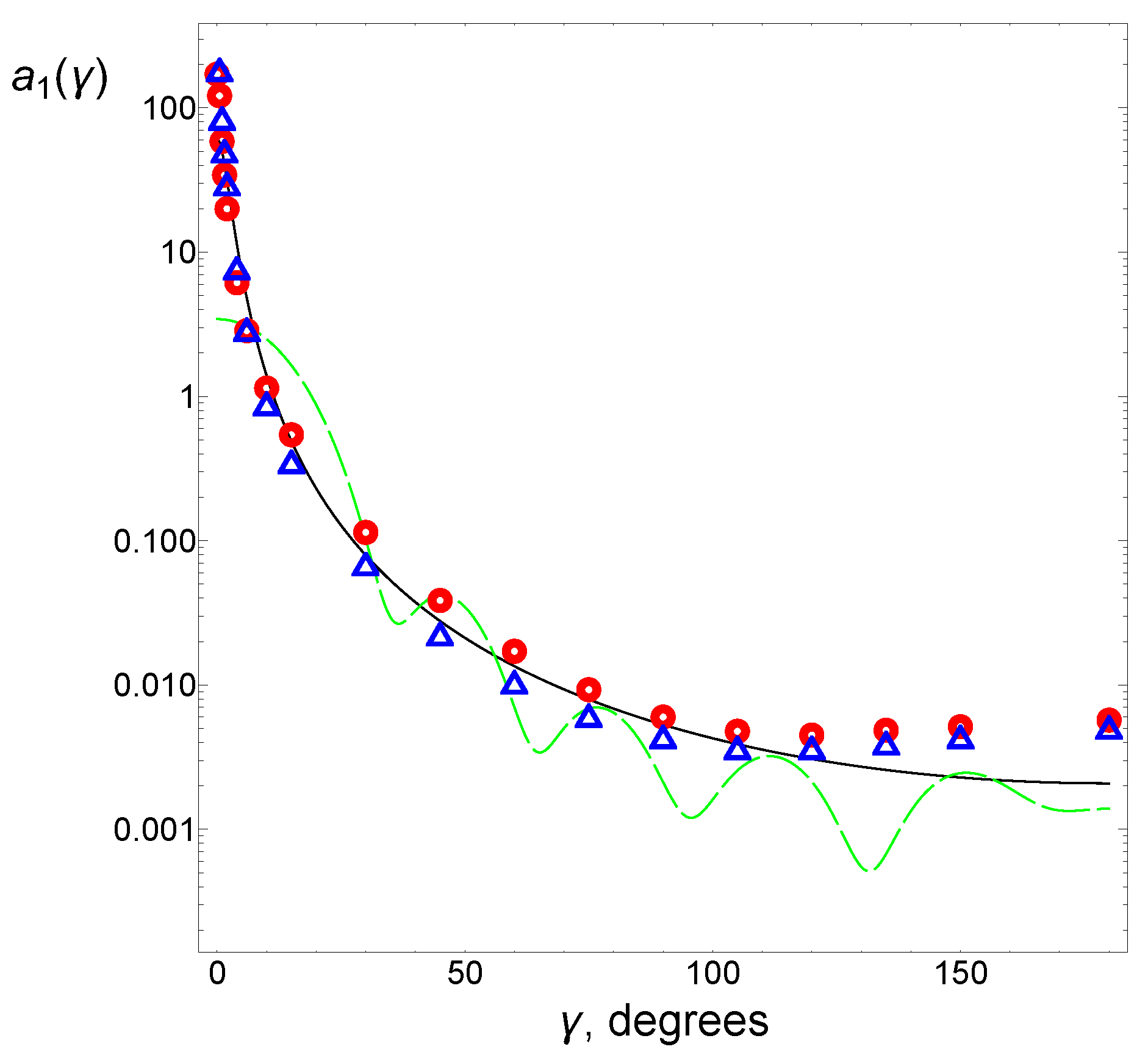
In sea water, single scattering of light by suspended particles is directed mainly forward, which is reflected in the angular profile of the phase function. Deflection of light by turbulent perturbations occurs through extremely small angles and does not affect the distribution of light scattered by suspended particles. In the radiative transfer theory, the effect of turbulence is not taken into consideration. Analysis of experimental data and numerical calculations (see, e.g., [1,7,9,15,47,48,59]) shows that the phase functions of sea water and other media with large inhomogeneities (e.g., aqueous suspension of polystyrene particles which is used to simulate scattering properties of sea water) fall off with increasing angle by a power law , where the exponent varies between and , and typical values of the angle are in the range – [1,7,9,15,47,48,59]. A number of examples of is illustrated in Figure 2.
For theoretical modeling the angular profile of single scattering in sea water, the Henyey-Greenstein phase function
and its modification proposed be Reynolds and McCormick [46]
are also widely used [7,9,15,21,50] (e.g., in Monte Carlo simulations [15], the phase function of sea water was fitted by Equation (18) with and ).
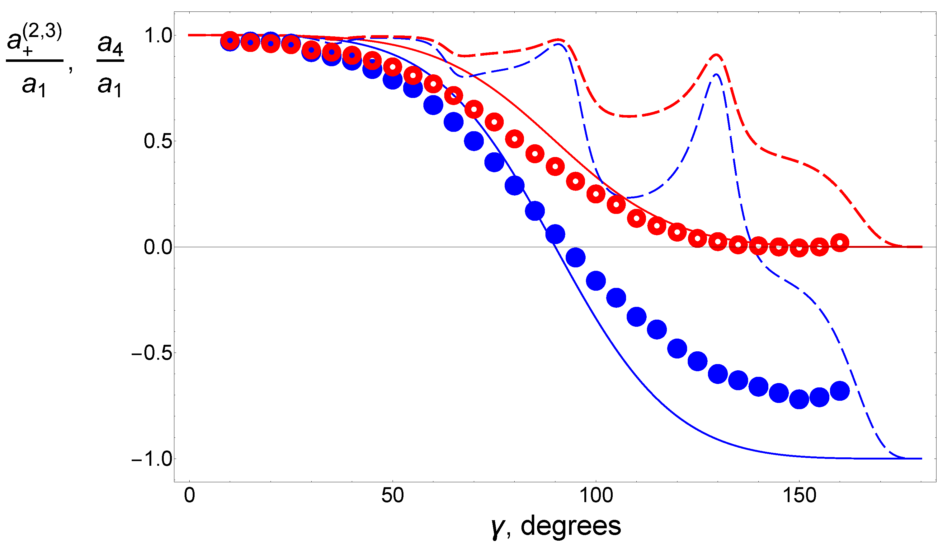
The scattering matrix elements of sea water can be inferred from data of measurements [49] and calculations (see, e.g., [61] and references therein). According to [49,62], the values of these elements for sea water are somewhat different from their Rayleigh values (see Equation (10)). The angular dependence of the elements and appearing in Equations (12) and (13) is shown in Figure 2. The data for sea water presented in Figure 3 can be approximated by the relations
where
The phase function is conveniently expanded in a series of Legendre polynomials
The expansion coefficients are used in solving the radiative transfer equation (see Appendix A and, e.g., [50]). The scattering matrix element appearing in Equation (13) can be expanded similarly. A somewhat different representation is valid for the scattering matrix element . The quantity entering into Equation (12) is expanded in a series of the generalized spherical functions [51]
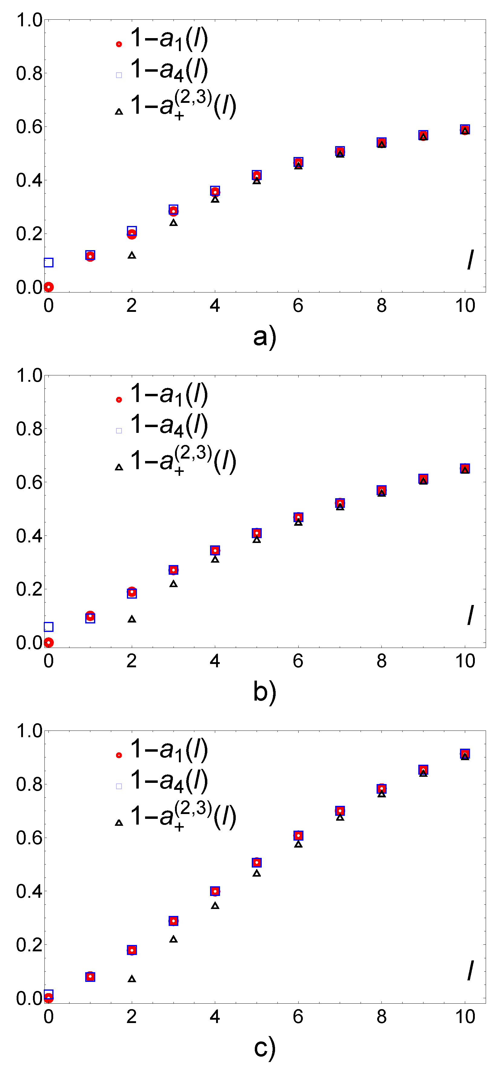
For the highly forward scattering medium such as sea water, the expansion coefficients , and differ from each other only at relatively small values of l. This is illustrated in Figure 4 where the results of numerical calculations of these coefficients for sea water and its imitations are presented.
4. Small-Angle Approximation. Scaling Relations
4.1. Distribution of Light Field in a Pulse
Multiple scattering of light in sea water occurs predominantly through small angles. This primarily relates to early arrival photons in the pulse. In this case, the radiative transfer Equations (11)–(13) can be from the outset transformed within the small-angle approximation.
To apply the small-angle approximation to Equation (11), we expand the coefficients on the left-hand-side of Equation (11) in a series in the small quantities and ( and are the projections of the unit vector on the x and y axises, ) and retain only the first nonvanishing terms. As a result, we arrive at the following equation [28]:
where and . The condition (14) takes the form
Using the Laplace transform with respect to the variable and the Fourier transform with respect to the angular variable , the solution of the problem (22) and (23) can be written as (see, e.g., [28,63]):
where and are the eigenvalues and normalized eigenfunctions of the equation
with
is the Bessel function. Equations (24) and (25) can be cosidered as small-angle versions of the expression (15) and the characteristic Equation (A4) (see Appendix A). Correspondingly, Equation (26) is a small-angle limit in the well-known expression for the coefficients of the phase function expansion in a series in the Legendre polynomials (see Equation (A7)).
The intensity of non-scattered light can be excluded from Equation (24) by subtracting from .
Within the small-angle approximation, the phase function (18) takes the form
In this case, the expansion of in powers of l begins with the term proportional to
where is the gamma-function. Under the assumption that the multiple scattering angles are greater than the characteristic single-scattering angle , only the first term in the expansion (28) should be taken into account (simultaneously, we neglect from here on the contribution from the non-scattered light, ). In this case, the eigenvalues can be scaled as
where is the -dependent numerical coefficient, and is the transport scattering coefficient, for the phase function (18) . Then the intensity can be expressed in terms of dimensionless variable . Integrating Equation (22) over angles and taking into account the dependence of the intensity on the variable , we can find the mean square of the angle at given z and t,
For early arrival photons, , only the minimum eigenvalue and, correspondingly, the first term in the sum (24) make a contribution to the intensity . In this case, the integral over p is governed by rather great values of p, . The inverse Laplace transform in Equation (24) can be performed using the stationary phase method (the saddle point is equal to , the numerical values of are given in Figure 5). As a result, the distribution of light field in the pulse can be presented in the form
where , and it is assumed that .
The approach based on Equations (22)–(25) can also be extended to a narrow beam geometry (see Appendix B).
The distribution (31) is valid for early arrival photons, including the peak of the pulse. The tail of the pulse () is described by the Laplace transform of the intensity at relatively small values of p, . In this case, we can take advantage of the results of calculations for relatively weak absorption, [64]. Generalizing the results [64] to the pulse propagation problem, we find that the integral-over-angle intensity decreases with increasing the ”excess” path as
where . Thus, the behavior of the temporal sweep of the pulse at relatively great values of the “excess” path is directly related to the angular profile of the phase functions at .
4.2. Degree of Polarization
For the basic modes of linear and circular polarizations, solutions of Equations (12) and (13) can also be presented in the form that is similar to Equation (24). The corresponding solutions differ from Equation (24) only by the specific eigenvalues, and , and the corresponding eigenfunctions, and .
In the case of highly forward multiple scattering, the values of and turn out to be close to provided that the value of p is rather great, . For such values of p, only the terms with (i.e., the minimum eigenvalues) make the main contribution. Therefore we can calculate the values of and analytically with a perturbation theory taking the solution of the scalar transfer Equation (25) as the first approximation. Within such an approach, the difference between the values of , and can be written in the form
where is the difference between and the Bessel transforms of the “effective” phase functions appearing in Equations (12) and (13).
The small-angle transfer equation for the basic mode of linear polarization differs from Equation (25) only by the “perturbation” term [35,36,44],
The first term in Equation (34) is responsible for the “geometrical” depolarization due to the Rytov effect. The second term describes the “dynamical” depolarization. Substituting Equation (34) into Equation (33), we obtain
where . When deriving Equation (35), we use the Gaussian ansatz for the eigenfunction and the relation .
For the basic mode of circular polarization, the difference is only due to the “dynamical” mechanism of depolarization. The value of turns out to be two times greater than appearing in (34) [35,36,44]. The quantity is determinate by
where . The results (35) and (36) rely on the small-angle phase function (27) and the Rayleigh approximation for the scattering matrix elements (see Equation (10)).
Evaluating the integral in Equation (24) and the integrals in the corresponding representations for the modes W and V by the saddle-point method, we obtain the expressions for the degree of linear and circular polarization of the pulse
where is determined by Equation (30). From Equations (37) and (38) it follows that the degree of polarization depends only on one dimensionless variable
and decreases with increasing the “excess” path .
5. Results of Numerical Calculations
The results obtained above in Section 3 and Section 4 can be validated using the numerical solution of the eigenvalue problem (see Appendix A) without resort to the small-angle approximation. In what follows it is assumed that all eigenvalues and eigenfunctions for the basic modes I, W and V correspond to the number .
First we outline the numerical results for . The p-dependence of at can be approximated by a power law,
The values of and for sea water (Kopelevich’s model [47,48]) and its imitation are given in Table 1. The calculations of were carried out with Equation (A4) (see Appendix A).
The eigenvalues , and , and the differences , as functions of are shown in Figure 6. For sea water, the results of measurements by Voss and Fry [49] were used for calculating the scattering matrix elements and . For the Henyey-Greenstein phase function, the calculations were carried out within the Rayleigh approximation (see Equation (10)). The calculations of and based on the Mie theory [60] underlie the results obtained for aqueous suspension of polystyrene spheres.
The angular dependence of the eigenfunctions , and is illustrated in Figure 7 for the reference case of the Henyey-Greenstein phase function. The difference between the eigenfunctions is small in the forward hemisphere, suggesting that the angular profile is unaffected by the initial polarization of light or, in other words, the decay of the initial polarization is virtually angle independent.
The contribution from the geometrical depolarization to is shown in Figure 8. This contribution is the main for aqueous suspension of relatively large polystyrene spheres (m, nm), and for the reference case involving the combination of the Henyey-Greenstein phase function with the Rayleigh scattering matrix and is comparatively modest for sea water. The features of the Voss-Fry scattering matrix [49] that are inherent in scattering by non-spherical particles make the dynamical depolarization principal for sea water. As p increases, and decreases according to a power law,
The numerical values of and are presented in Table 2. For the latter two lines of Table 2 the values of and coincide to the corresponding values of , correlating with Equations (35) and (36).
6. Discussion
The results obtained above give an insight into the distribution of light field in the pulse and enable calculating semi-analytically its main characteristics, including the polarization state, in sea water.
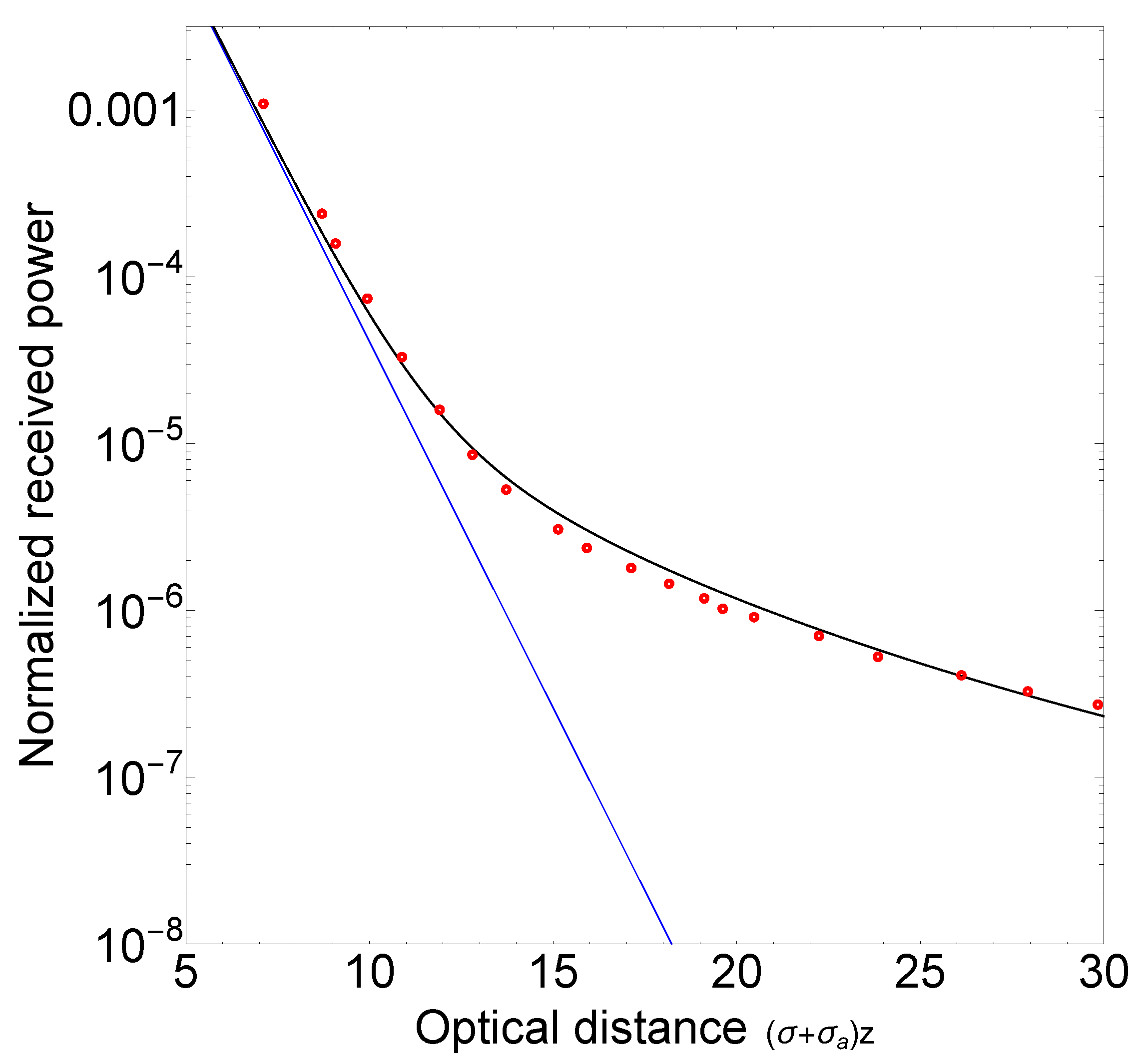
For the intensity of radiation in the pulse, the small-angle approximation can be applied in combination with an adequate parametrization of the sea water phase function. A peculiarity of light scattering by sea water is that the wings of the phase function at ( is of the order of a few degrees) fall off rather slowly, according to a power law. Therefore, the parametrization such as the Henyey-Greenstein function or the Reynolds-McCormick one grasps the key feature of light scattering by sea water in the forward hemisphere. This is confirmed by the data presented in Figure 2 and Figure 4. Additionally, to validate the power-law approximation (28) in application to a realistic situation, we compare the results of our calculations with experiment [7]. Substituting Equation (28) with the same parameters as in Monte Carlo simulation [7,9] (i.e., , ) to the small-angle solution of the transfer equation (see, e.g., [21]), we obtain the attenuation curve which agrees with the experimental data (see Figure 9). The relative contribution of multiple-scattered radiation to the received signal increases with the optical distance, resulting in the decrease of the attenuation rate as compared to Beer’s law.
Using the power-law approximation for the phase function, we can represent the distribution of light field in the pulse in the self-similar form as a function of dimensionless variables (see Equations (31) and (32)). These variables are certain combinations of the “excess” path , the transport scattering coefficient , the source-receiver distance z and the exponent appearing in the parametrization of the phase function. Correspondingly, the main characteristics of the light field distribution (the effective time spread, dispersion in angles and etc.) are expressed in terms of these variables.
The important result for the variance of the angular distribution of light field, (see Equation (30)), enables controlling the validity of the small-angle approximation at given z and t.
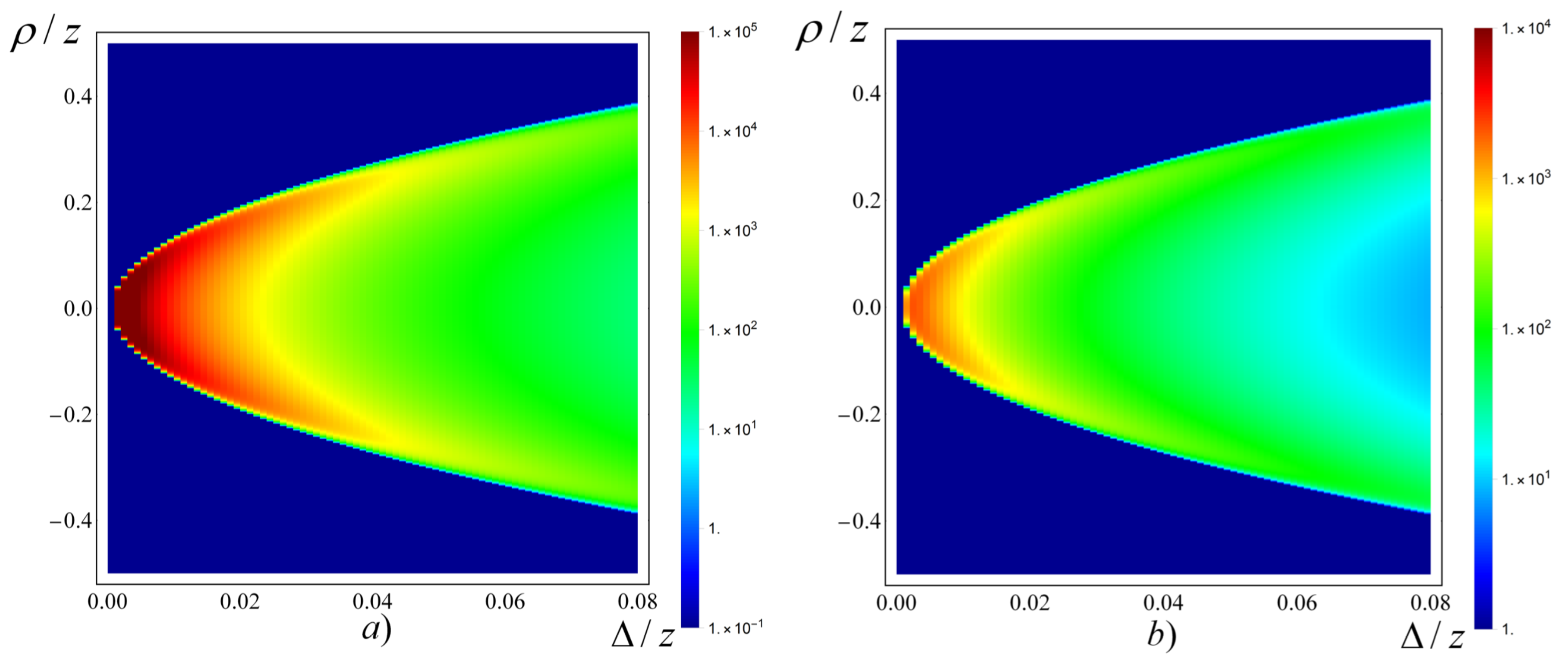
From the results obtained it follows that the peak in the temporal sweep of the pulse is observed at small values of the “excess” path, , or, for a narrow beam, ( is the transverse displacement from the beam axis, see Appendix B). This is illustrated in Figure 10 where the distribution of light field in the forward direction and the integral-over-angle distribution are shown. The latter correlates well with the Monte Carlo simulation data [11] (see Figures 3 and 4 in [11]).
The calculations of light field with the use of the numerical results outlined in Section 5 are performed in the following way. First, the integral over p in Equation (15) is evaluated by the stationary phase (or saddle-point) method, and, as before, only the contribution from the minimum eigenvalue is taken into account. The saddle-point is sought from the equation
The value of can be found using the power-law approximation for (see Equation (40)) or, directly, from the numerical values (see Figure 6). In the latter case, the results obtained are valid even beyond the small-angle approximation. Further the integral in Equation (15) is calculated routinely (all p-dependent factor appearing in Equation (15) are taken at the saddle-point ).
Our approach to calculating the light field distribution in the pulse differs from the analytical solutions proposed for the same problem previously (see, e.g., [18,20,22,23,24,25,26,27,29,33]) in that the specific angular profile of the sea water phase function is allowed for in our calculations.
The basic modes of linear and circular polarization, and the corresponding degree of polarization are calculated similarly to the light field distribution. The degree of polarization can be written as
where and is the root of Equation (42). The numerical values of and as functions of p are given in Figure 6. Their analytical parametrization is described by Equations (35) and (36) or (41).
The applicability of the expression for the degree of polarization in the form (43) is not limited by the small-angle approximation.
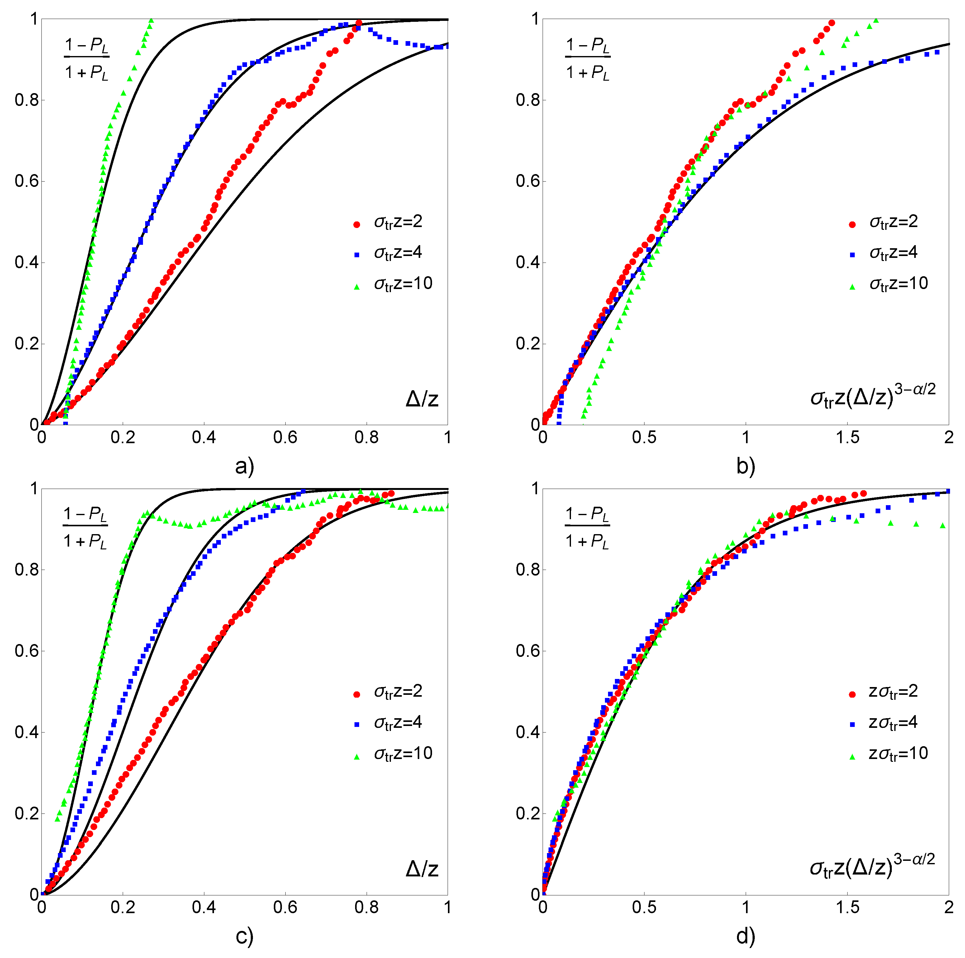
The results of comparison of our calculations with data of Monte Carlo simulations for aqueous suspension of polystyrene spheres [17] are shown in Figure 11. The numerical simulation [17] was carried out for the linearly polarized pulse propagating through a plane slab of different transport optical thickness . Depolarization ratio was presented in [17] as a function of the normalized “excess path” . When going from to novel variable (see Equation (39)) we obtain virtually universal pattern of the simulation data (see Figure 11b,d). The agreement between our calculations and the data [17] shows possibility of application of the power-law parametrization (41) to realistic cases.
As noted in Section 2.2 (see also [36,45]), two mechanisms underlie the depolarization of light in scattering media. For sea water, as follows from the numerical results presented in Figure 6 and Figure 8, the dynamical mechanism of depolarization proves to be dominant. This is due to specific feature of the Voss-Fry scattering matrix at relatively small scattering angles . From the Voss-Fry measurements (see Figure 3 and also the approximation (19) and the parametrization proposed in [62]) it follows that, for small , both and are proportional to . In the Rayleigh approximation (see Equation (10)) and in the case of aqueous suspension of polystyrene spheres, contrastingly, these quantities are proportional to . This distinction can be explained by the contribution of large non-spherical particles to the scattering matrix of sea water. For this reason the effect of circular polarization memory that is typical for aqueous suspension of polystyrene spheres (see, e.g., [36,45,65,66,67]) can not be observed in propagation of light through sea water. The linearly and circularly polarized beams are depolarized equally (see Figure 6).
7. Conclusions
We have studied the distribution of light field and the degree of light polarization in transmission of a pulsed beam through sea water. A novel method has been proposed that enables calculating the distribution and the degree of polarization of light field in a pulsed signal, based on a numerical solution of the eigenvalue problem for the basic modes of the VRTE. The small-angle approximation underlies our analytical results that rely also on the power-law parametrization of the phase function and on the Rayleigh scattering matrix. The numerical calculations beyond this approximation have been performed for the actual data on the sea water phase function and the scattering matrix. The eigenvalues entering into the expressions for the Laplace transform of the basic modes with respect to the time variable have been shown to be written in a power-law form. This enables expressing the light field distribution and the degree of polarization in the pulse in terms of dimensionless variables in a self-similar form. The variance of the multiple-scattering angle has been shown to be proportional to the ratio of the “excess” path to the source-receiver distance z, justifying the application of the small-angle approximation to calculating the early arrival component of light field () in the pulse. We have also found that the depolarization properties of sea water differ from those (see, e.g., [36,45,65,66,67]) of aqueous suspension of polystyrene spheres. Contrary to [36,45,65,66,67], as follows from our calculations based on the actual data on the sea water scattering matrix [49], the depolarization rates for linearly and circularly polarized pulses prove to be virtually equal to each other. This can be explained by scattering from non-spherical particles suspended in sea water.
The analysis and results presented above can find application to the problems involving propagation of non-stationary laser beams through sea water, such as underwater communication, imaging and remote sensing.
Author Contributions
Conceptualization, E.E.G., A.I.K. and D.B.R.; methodology, E.E.G., A.I.K. and D.B.R.; software, K.A.K.; validation, K.A.K.; writing–original draft preparation, E.E.G. and D.B.R.; writing–review and editing, E.E.G. and D.B.R.; visualization, K.A.K. All authors have read and agreed to the published version of the manuscript.
Funding
This research received no external funding.
Acknowledgments
We thank O.V. Kopelevich for his interest in the work and valuable advice. E.E.G. is grateful to L.S. Dolin and A.G. Luchinin for stimulating discussions. D.B.R. would like to express his gratitude to Yu.A. Goldin, V.V. Marinuyk, V.S. Remizovich, S.V. Sheberstov and the late A.K. Zakharov for numerous helpful discussions and cooperation.
Conflicts of Interest
The authors declare no conflict of interest.
Appendix A. Eigenvalue Problem for the Basic Modes
The elements of the phase matrix (6) can be expanded in the generalized spherical functions [51,52]. Therefore, solutions to Equations (11)–(13) can be sought in the form of series in these functions as well [52]. In the scalar transfer theory, this approach is known as -approximation [2,21,50]. As applied to the VRTE, expansion in the generalized spherical functions was originally proposed in [52], and used then in many numerical and analytical calculations ( see, e.g., [36,45] and references therein).
The eigenfunctions , and (see Equation (15)) can be represented as [36,45]
where and are the Legendre polynomials and the generalized spherical functions, respectively. Detailed properties of can be found in [51].
Substituting expansions of the type of Equation (15) into Equations (11)–(13) and taking into account the expansions of the scattering matrix elements in the generalized spherical functions (see Equations (20) and (21)) we arrive at the following equations for the coefficients entering into Equations (A1)–(A3) and the corresponding eigenvalues:
where
Solutions to Equations (A4)–(A6) are found numerically with the use of truncating at some . In such a way, we find a set of the eigenvalues and the eigenfunctions for each mode, I, W and V.
Appendix B. Generalization to a Narrow Beam
The results obtained in Section 4.1 can be directly extended to the case of a narrow beam. The transfer Equation (22) should be replaced by
where and the collision integral on the right-hand-side is the same as in Equation (22). The source (23) is changed for
Then the distribution of light field in the beam can be written in the form
where coincides with the right-hand-side of Equation (24). Taking into account only the first term in the expansion (24) and using the Gaussian ansatz for corresponding eigenfunction, we obtain
where , and (see Equation (31)). Equation (A11) is valid for early arrival photons, including the peak of the pulse (). The “excess” path appearing in Equation (31) is replaced now by which is the approximation of the difference .
References
- Monin, A.S. (Ed.) Optika Okeana (Oceanic Optics); Nauka: Moscow, Russia, 1983; Volume 2. [Google Scholar]
- Zege, E.P.; Ivanov, A.P.; Katsev, I.L. Image Transfer through a Scattering Medium; Springer: Berlin/Heidelberg, Germany, 1991. [Google Scholar]
- Jaruwatanadilok, S. Underwater wireless optical communication channel modeling and performance evaluation using vector radiative transfer theory. IEEE J. Ser. Areas Commun. 2008, 26, 1620–1627. [Google Scholar] [CrossRef]
- Cochenour, B.M.; Mullen, L.J.; Laux, A.E. Characterization of the beam-spread function for underwater wireless optical communications links. IEEE J. Ocean. Eng. 2008, 33, 513–521. [Google Scholar] [CrossRef]
- Mullen, L.; Alley, D.; Cochenour, B. Investigation of the effect of scattering agent and scattering albedo on modulated light propagation in water. Appl. Opt. 2011, 1396–1404. [Google Scholar] [CrossRef] [PubMed]
- Cochenour, B.; Mullen, L.; Muth, J. Temporal response of the underwater optical channel for high-bandwidth wireless laser communications. IEEE J. Ocean. Eng. 2013, 38, 730–742. [Google Scholar] [CrossRef]
- Cox, W.; Muth, J. Simulating channel losses in an underwater communication system. J. Opt. Soc. Am. 2014, 31, 920–934. [Google Scholar] [CrossRef] [PubMed]
- Zeng, Z.; Fu, S.; Zhang, H.; Dong, Y.; Cheng, J. A survey of underwater optical wireless communications. IEEE Commun. Surv. Tutor. 2017, 19, 204–238. [Google Scholar] [CrossRef]
- Sahu, S.K.; Shanmugam, P. A theoretical study on the impact of particle scattering on the channel characteristics of underwater optical communication system. Opt. Commun. 2018, 408, 3–14. [Google Scholar] [CrossRef]
- Luchinin, A.G.; Dolin, L.S. Model of an underwater imaging system with a complexly modulated illumination beam. Izv. Atmos. Ocean. Phys. 2014, 50, 411–419. [Google Scholar] [CrossRef]
- Luchinin, A.G.; Kirillin, M.Y. Temporal and frequency characteristics of a narrow light beam in sea water. Appl. Opt. 2016, 55, 7756–7762. [Google Scholar] [CrossRef]
- Walker, R.E.; McLean, J. Lidar equations for turbid media with pulse stretching. Appl. Opt. 1999, 38, 2384–2397. [Google Scholar] [CrossRef]
- Vasilkov, A.P.; Goldin, Y.A.; Gureev, B.A.; Hoge, F.E.; Swift, R.N.; Wright, C.W. Airborne polarized lidar detection of scattering layers in the ocean. Appl. Opt. 2001, 40, 4353–4364. [Google Scholar] [CrossRef] [PubMed]
- Luchinin, A.G. Theory of underwater lidar with a complex modulated illumination beam. Izv. Atmos. Ocean. Phys. 2012, 48, 663–671. [Google Scholar] [CrossRef]
- Lerner, R.M.; Summers, J.D. Monte-Carlo description of time-resolved and space-resolved multiple forward scatter in natural water. Appl. Opt. 1982, 21, 861–869. [Google Scholar] [CrossRef] [PubMed]
- Zakharov, A.K.; Goldin, Y.A. The Monte Carlo calculation of the structure of narrow non-stationary light beams in sea water up to a large optical depth. Izv. Akad. Nauk SSSR Fiz. Atmos. Okeana 1986, 22, 533–540. [Google Scholar]
- Bruscaglioni, P.; Zaccanti, G.; Wei, Q. Transmission of a pulsed polarized light beam through thick turbid media: Numerical results. Appl. Opt. 1993, 32, 6142–6150. [Google Scholar] [CrossRef]
- McLean, J.; Freeman, J.D.; Walker, R.E. Beam spread function with time dispersion. Appl. Opt. 1998, 37, 4701–4711. [Google Scholar] [CrossRef]
- Ishimaru, A.; Jaruwatanadilok, S.; Kuga, Y. Polarized pulse waves in random duscrete scatterers. Appl. Opt. 2001, 40, 5495–5502. [Google Scholar] [CrossRef]
- Luchinin, A.G. Spatial spectrum of a narrow sine-wave-modulated light beam in an anisotropically scattering medium. Izv. Acad. Sci. USSR Atmos. Ocean. Phys. 1974, 10, 1312–1317. [Google Scholar]
- Ishimaru, A. Wave Propagation and Scattering in Random Media; Institute of Electrical and Electronics Engineers: New York, NY, USA, 1997. [Google Scholar]
- Dolin, L.S. Solution of the radiation transfer equation in a small-angle approximation for a stratified turbid medium with photon path dispersion taken into account. Izv. Acad. Sci. USSR Atmos. Ocean. Phys. 1980, 16, 55–64. [Google Scholar]
- Dolin, L.S. Self-similar approximation in the theory of multiple strongly anisotropic light scattering. Dokl. Akad. Nauk SSSR 1981, 260, 1344–1347, [Sov. Phys. Dokl. 1981, 26, 976–979]. [Google Scholar]
- Dolin, L.S. Passage of a pulsed light signal through an absorbing medium with strongly anisotropic scattering. Izv. Vyss. Uchebnykh Zaved. Radiofiz. 1983, 26, 220–228. [Google Scholar] [CrossRef]
- Remizovich, V.S.; Rogozkin, D.B.; Ryazanov, M.I. Propagation of a narrow modulated light beam in a scattering medium: The effect of fluctuations in path lengths of multiply scattered photons. Radiophys. Quantum Electron. 1982, 25, 639–645. [Google Scholar] [CrossRef]
- Remizovich, V.S.; Rogozkin, D.B.; Ryazanov, M.I. Propagation of an optical signal in matter with large-scale random inhomogeneities with allowance for fluctuations of the photon paths in multiple scattering. Izv. Akad. Nauk SSSR Fiz. Atmos. Okeana 1982, 18, 623–631. [Google Scholar]
- Remizovich, V.S.; Rogozkin, D.B.; Ryazanov, M.I. Propagation of a light-flash signal in a turbid medium. Izv. Acad. Sci. USSR Atmos. Ocean. Phys. 1983, 19, 796–801. [Google Scholar]
- Rogozkin, D.B. Propagation of a light pulse in a medium with strongly anisotropic scattering. Izv. Acad. Sci. USSR Atmos.Ocean. Phys. 1987, 23, 275–281. [Google Scholar]
- van de Hulst, H.C.; Kattawar, G.W. Exact spread function for a pulsed collimated beam in a medium with small-angle scattering. Appl. Opt. 1994, 33, 5820–5829. [Google Scholar] [CrossRef]
- Gorodnichev, E.E.; Rogozkin, D.B. Multiple small-angle scattering of an optical pulse in turbid media: Polarization characteristics. Izv. Atmos. Ocean. Phys. 1997, 33, 74–81. [Google Scholar]
- Gorodnichev, E.E.; Ivliev, S.V.; Kuzovlev, A.I.; Rogozkin, D.B. Depolarization of light in the pulse transmission through the medium with large inhomogeneities. Laser Phys. 2010, 20, 2021–2028. [Google Scholar] [CrossRef]
- Gorodnichev, E.E.; Ivliev, S.V.; Kuzovlev, A.I.; Rogozkin, D.B. Transillumination of highly scattering media by polarized light. Light Scatt. Rev. 2013, 8, 317–362. [Google Scholar]
- Luchinin, A.G.; Dolin, L.S. On dispersive properties of photon density waves in anisotropic scattering medium. Radiophys. Quantum Electron. 2016, 59, 145–152. [Google Scholar] [CrossRef]
- Gorodnichev, E.E.; Kuzovlev, A.I.; Rogozkin, D.B. Small-angle multiple scattering of polarized light in turbid media. Izv. Atmos. Ocean. Phys. 2003, 39, 333–345. [Google Scholar]
- Gorodnichev, E.E.; Kuzovlev, A.I.; Rogozkin, D.B. Multiple scattering of polarized light in turbid media with large particles. Light Scatt. Rev. 2006, 291–338. [Google Scholar] [CrossRef]
- Gorodnichev, E.E.; Kuzovlev, A.I.; Rogozkin, D.B. Multiple scattering of polarized light in a turbid medium. JETP 2007, 104, 319–341. [Google Scholar] [CrossRef]
- Zege, E.P.; Chaykovskaya, L.I. Peculiarities of transfer of polarized radiation in media with highly anisotropic scattering. Zh. Prikl. Spektrosk. 1986, 44, 996–1004. [Google Scholar]
- Gorodnichev, E.E.; Kuzovlev, A.I.; Rogozkin, D.B. Propagation of a narrow beam of polarized light in a random medium with large-scale inhomogeneities. Laser Phys. 2000, 10, 1236–1243. [Google Scholar]
- Gorodnichev, E.E.; Kuzovlev, A.I.; Rogozkin, D.B. Influence of the inhomogeneity properties on the depolarization of multiply scattered light in a turbid medium. In Proceedings of the International Radiation Symposium IRS 2000: Current Problems in Atmospheric Radiation, St Petersberg, Russia, 24–29 July 2001; Smith, W.L., Timofeev, Y.M., Eds.; Deepak: Hampton, VA, USA, 2001; pp. 287–290. [Google Scholar]
- Demos, S.G.; Alfano, R.R. Temporal gating in highly scattering media by the degree of optical polarization. Opt. Lett. 1996, 21, 161–163. [Google Scholar] [CrossRef]
- Wang, X.; Wang, L.V.; Sun, C.-W.; Yang, C.-C. Polarized light propagation through scattering media: Time-resolved Monte Carlo simulations and experiments. J. Biomed. Opt. 2003, 8, 608–617. [Google Scholar] [CrossRef] [Green Version]
- Ni, X.; Xing, Q.; Cai, W.; Alfano, R.R. Time-resolved polarization to extract coded information from early ballistic and snake signals through turbid media. Opt. Lett. 2003, 28, 343–345. [Google Scholar] [CrossRef]
- Horinaka, H.; Hashimoto, K.; Wada, K.; Cho, Y.; Osawa, M. Extraction of quasi-straightforward-propagating photons from diffused light transmitting through a scattering medium by polarization modulation. Opt. Lett. 1995, 20, 1501–1503. [Google Scholar] [CrossRef] [PubMed]
- Gorodnichev, E.E.; Kuzovlev, A.I.; Rogozkin, D.B. Depolarization of light in small-angle multiple scattering in random media. Laser Phys. 1999, 9, 1210–1227. [Google Scholar]
- Gorodnichev, E.E.; Kuzovlev, A.I.; Rogozkin, D.B. Depolarization coefficients of light in multiply scattering media. Phys. Rev. 2014, 90, 043205. [Google Scholar] [CrossRef]
- Reynolds, L.; McCormick, N.J. Approximate two-parameter phase function for light scattering. JOSA 1980, A70, 1206–1212. [Google Scholar] [CrossRef]
- Kopelevich, O.V. Application of data on seawater light scattering for the study of marine particles: A selective review focusing on Russian literature. Geo-Mar. Lett. 2012. [Google Scholar] [CrossRef]
- Hultrin, V.I. Absorption and scattering of light in natural waters. Light Scatt. Rev. 2006, 445–486. [Google Scholar] [CrossRef]
- Voss, K.J.; Fry, E.S. Measurement of the Mueller matrix for ocean water. Appl. Opt. 1984, 23, 4427–4439. [Google Scholar] [CrossRef] [PubMed]
- van de Hulst, H.C. Multiple Light Scattering; Academic Press: New York, NY, USA, 1981. [Google Scholar]
- Mishchenko, M.I.; Travis, L.D.; Lacis, A.A. Multiple Scattering of Light by Particles; Cambridge University: Cambridge, UK, 2006. [Google Scholar]
- Kuscer, I.; Ribaric, M. Matrix formalism in the theory of diffusion of light. Opt. Acta 1959, 6, 42–57. [Google Scholar] [CrossRef]
- Zege, E.P.; Chaikovskaya, L.I. Approximate theory of linearly polarized light propagation through a scattering medium. JQSRT 2000, 66, 413–435. [Google Scholar] [CrossRef]
- Case, K.M.; Zweifel, P.F. Linear Transport Theory; Addison-Wesley Publishing Company: Boston, MA, USA, 1967; Chapter 7. [Google Scholar]
- Strohbenh, J.W.; Clifford, S.F. Polarization and angle-of-arrival fluctuatins for a plane wave propagated through a turbulent medium. IEEE Trans. Anten. Propag. 1967, 15, 416–421. [Google Scholar] [CrossRef]
- Tatarskii, V.I. Depolarization of a light beam in a turbulent atmosphere. Izv. Vyssh. Uchebn. Zaved. Radiofiz. 1967, 10, 1762–1763. [Google Scholar]
- Kravtsov, Y.A. “Geometrical” depolarization of light in a turbulent atmosphere. Izv. Vyssh. Uchebn. Zaved. Radiofiz. 1970, 13, 281–284. [Google Scholar]
- Landau, L.D.; Lifshitz, E.M. Electrodynamics of Continuous Media; Pergamon: New York, NY, USA, 1960. [Google Scholar]
- Mobley, C.D.; Gentili, B.; Gordon, H.R.; Jin, Z.; Kattawar, G.W.; Morel, A.; Reinersman, P.; Stamnes, K.; Stavn, R.H. Comparison of numerical models for computing underwater light fields. Appl. Opt. 1993, 32, 7484–7504. [Google Scholar] [CrossRef] [PubMed] [Green Version]
- Laven, P. Simulation of rainbows, coronas, and glories by use of Mie theory. Appl. Opt. 2003, 42, 436–444. [Google Scholar] [CrossRef] [PubMed]
- Sun, B.; Kattawar, G.W.; Yang, P.; Zhang, X. A brief review of Muller matrix calculations associated with oceanic particles. Appl. Sci. 2018, 8, 2686. [Google Scholar] [CrossRef] [Green Version]
- Kokhanovsky, A.A. Parameterization of the Mueller matrix of oceanic waters. J. Geophys. Res. 2003, 108, 3175. [Google Scholar] [CrossRef]
- Alexandrov, M.D.; Remizovich, V.S.; Rogozkin, D.B. Multiple light scattering in a two-dimensional medium with large scatterers. J. Opt. Soc. Am. 1993, 10, 2602–2610. [Google Scholar] [CrossRef] [Green Version]
- Marinyuk, V.V.; Rogozkin, D.B.; Sheberstov, S.V. Propagation of a light beam in an absorbing medium with large-scale inhomogeneities. Opt. Spectrosc. 2014, 117, 102–114. [Google Scholar] [CrossRef]
- Bicout, D.; Brosseau, C.; Martinez, A.S.; Schmitt, J.M. Depolarization of multiply scattered waves by spherical diffusers: Influence of the size parameter. Phys. Rev. 1994, 49, 1767–1770. [Google Scholar] [CrossRef]
- Xu, M.; Alfano, R.R. Circular polarization memory of light. Phys. Rev. 2005, 72, 065601. [Google Scholar] [CrossRef]
- Dark, J.; Kim, A.D. Asymptotic theory of circular polarization memory. J. Opt. Soc. Am. 2017, 34, 1642–1650. [Google Scholar] [CrossRef] [PubMed]
Figure 1.
Scattering geometry.

Figure 2.
Examples of the angular dependence of the scattering phase function for sea water. The results obtained with Kopelevich’s model [47,48] and analytical parametrization (18) (, [15]) are depicted by symbols (∘, , , ) and solid line, respectively. For comparison, the results of calculations with code [60] for aqueous suspension of polystyrene spheres (diameter m, wavelength nm) are shown by dashed line.

Figure 3.
Ratios and as functions of scattering angle for sea water [49] (symbols ∘ and •, respectively). For comparison, the Rayleigh values (solid curves) and the results of calculations with code [60] for aqueous suspension of polystyrene spheres (diameter m, wavelength nm, dashed curves) are also shown.

Figure 4.
Quantities (∘), (□), () as functions of l. The calculations were performed for (a) sea water (Kopelevich’s model [47,48], , and scattering matrix [49]), (b) the Henyey-Greenstein phase function and the Rayleigh scattering matrix, and (c) aqueous suspension of polystyrene spheres (diameter m and wavelength nm).

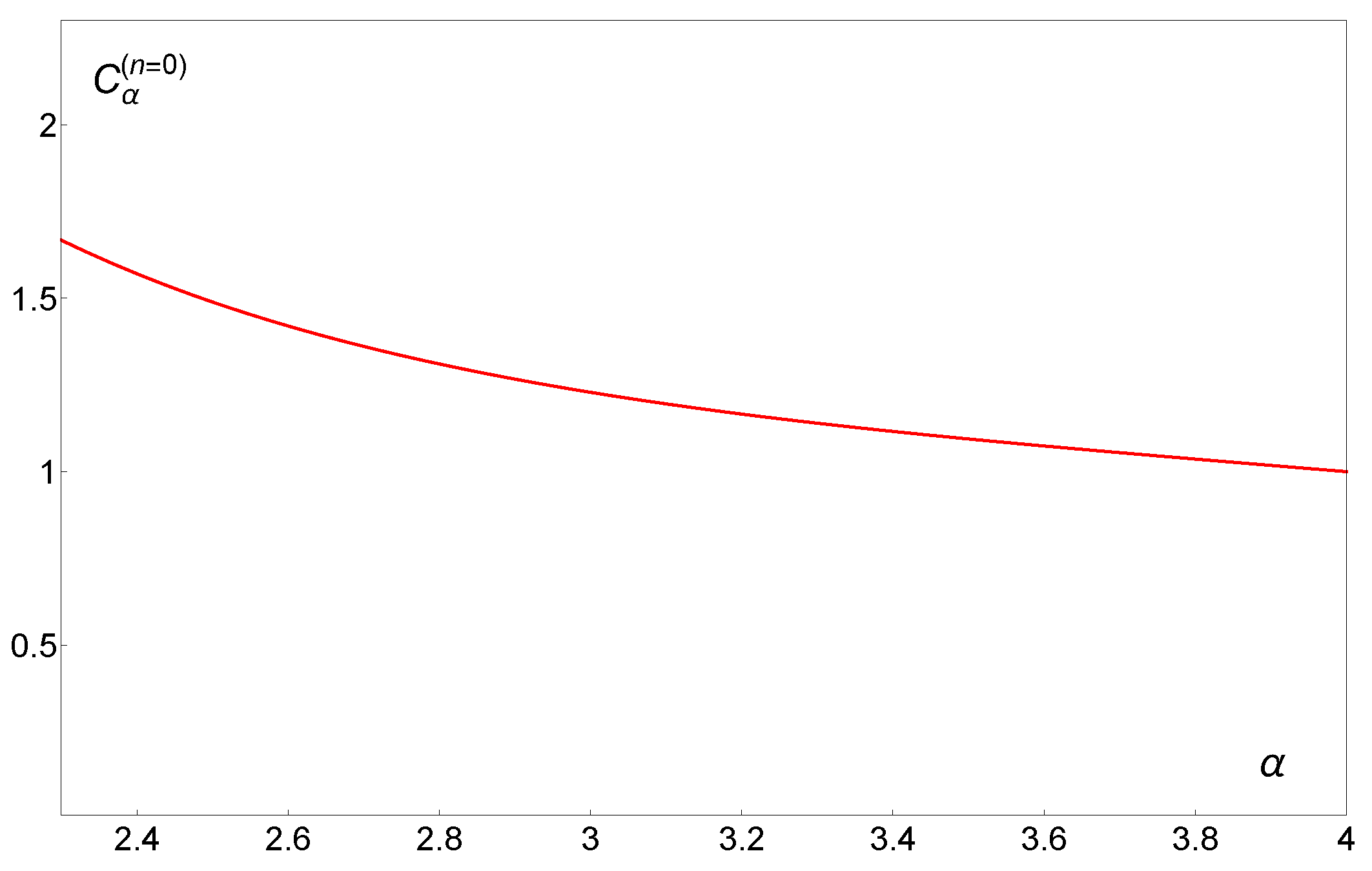
Figure 5.
Coefficient as a function of index .

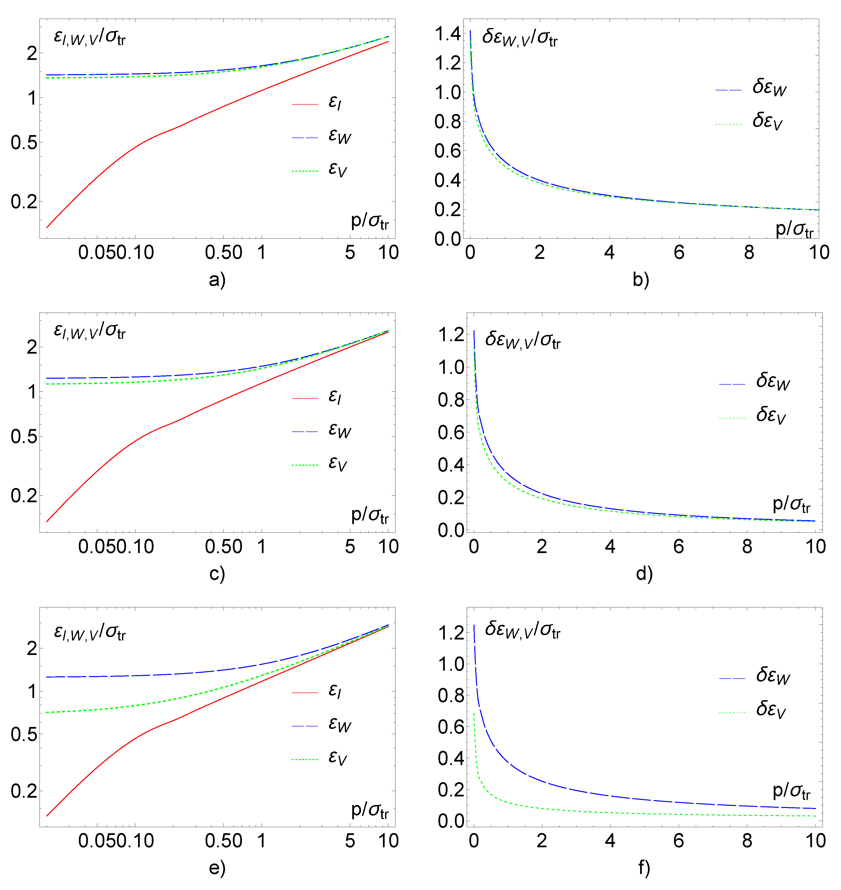
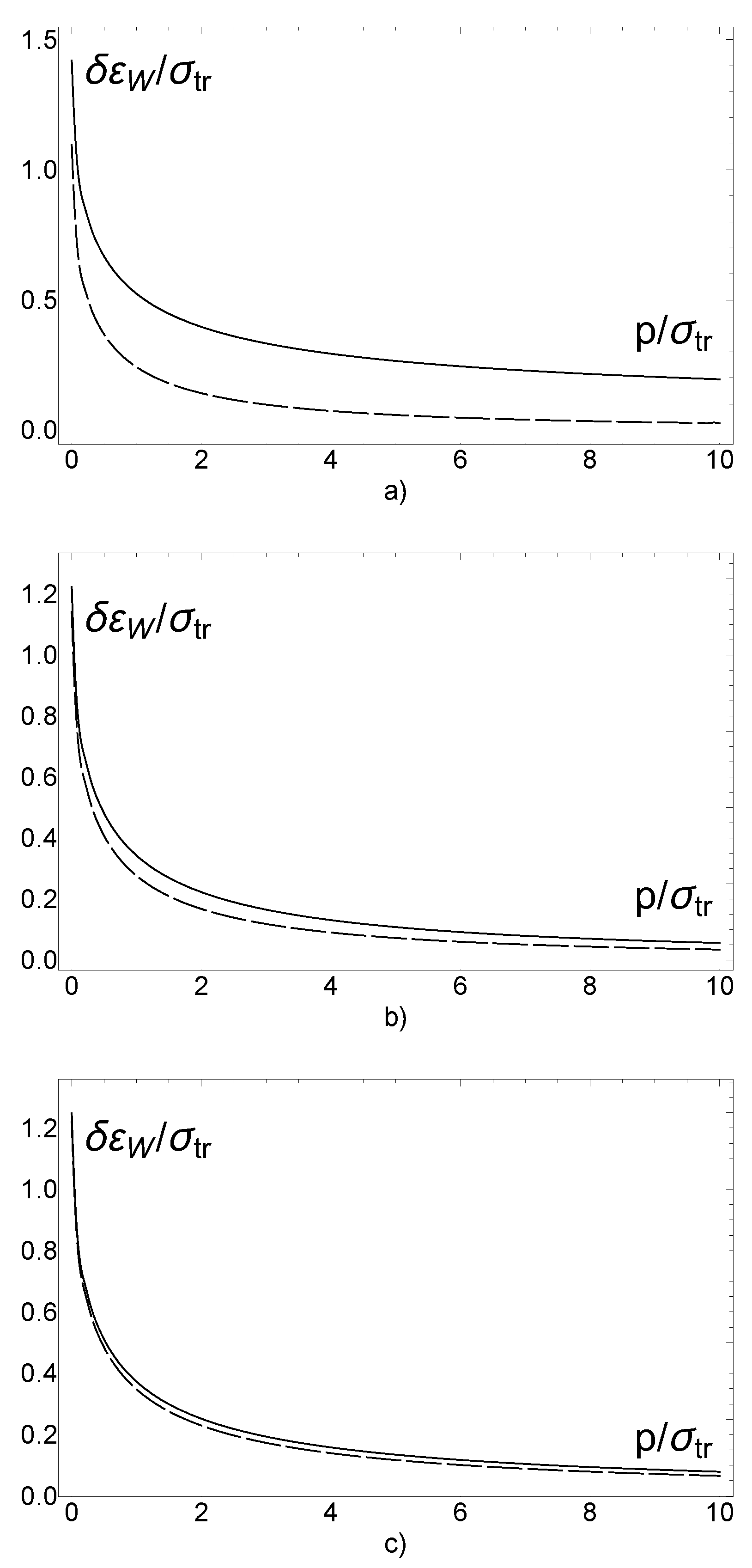
Figure 6.
Eigenvalues , and (solid, dashed and dotted lines, respectively) and differences and (dashed and dotted lines, respectively) versus p. The numerical calculations were carried out for (a,b) sea water, , (c,d) Henyey-Greenstein phase function/Rayleigh scattering matrix, and (e,f) aqueous suspension of polystyrene spheres (m, nm).

Figure 7.
Example of the angular dependence , and (solid, dashed and dotted lines). The numerical calculations were carried out for the Henyey-Greenstein phase function () combined with the Rayleigh scattering matrix (from upper to lower curves, and 5).
Figure 7.
Example of the angular dependence , and (solid, dashed and dotted lines). The numerical calculations were carried out for the Henyey-Greenstein phase function () combined with the Rayleigh scattering matrix (from upper to lower curves, and 5).

Figure 8.
Comparison of and (solid and dashed lines, respectively). The cases are the same as in Figure 6.
Figure 8.
Comparison of and (solid and dashed lines, respectively). The cases are the same as in Figure 6.

Figure 9.
Normalized received power versus optical source-receiver distance (symbols [7]). The results of calculations within the small-angle approximation for the Henyey-Greenstein phase function () are shown by solid curve. The attenuation of non-scattered radiation, Beer’s law, is displayed by straight line.

Figure 10.
Light field distribution in a pulsed beam on the plane (, ) for direction (a) and upon integrating over angles (b). The calculations were carried out for , and the phase function of sea water ().
Figure 10.
Light field distribution in a pulsed beam on the plane (, ) for direction (a) and upon integrating over angles (b). The calculations were carried out for , and the phase function of sea water ().

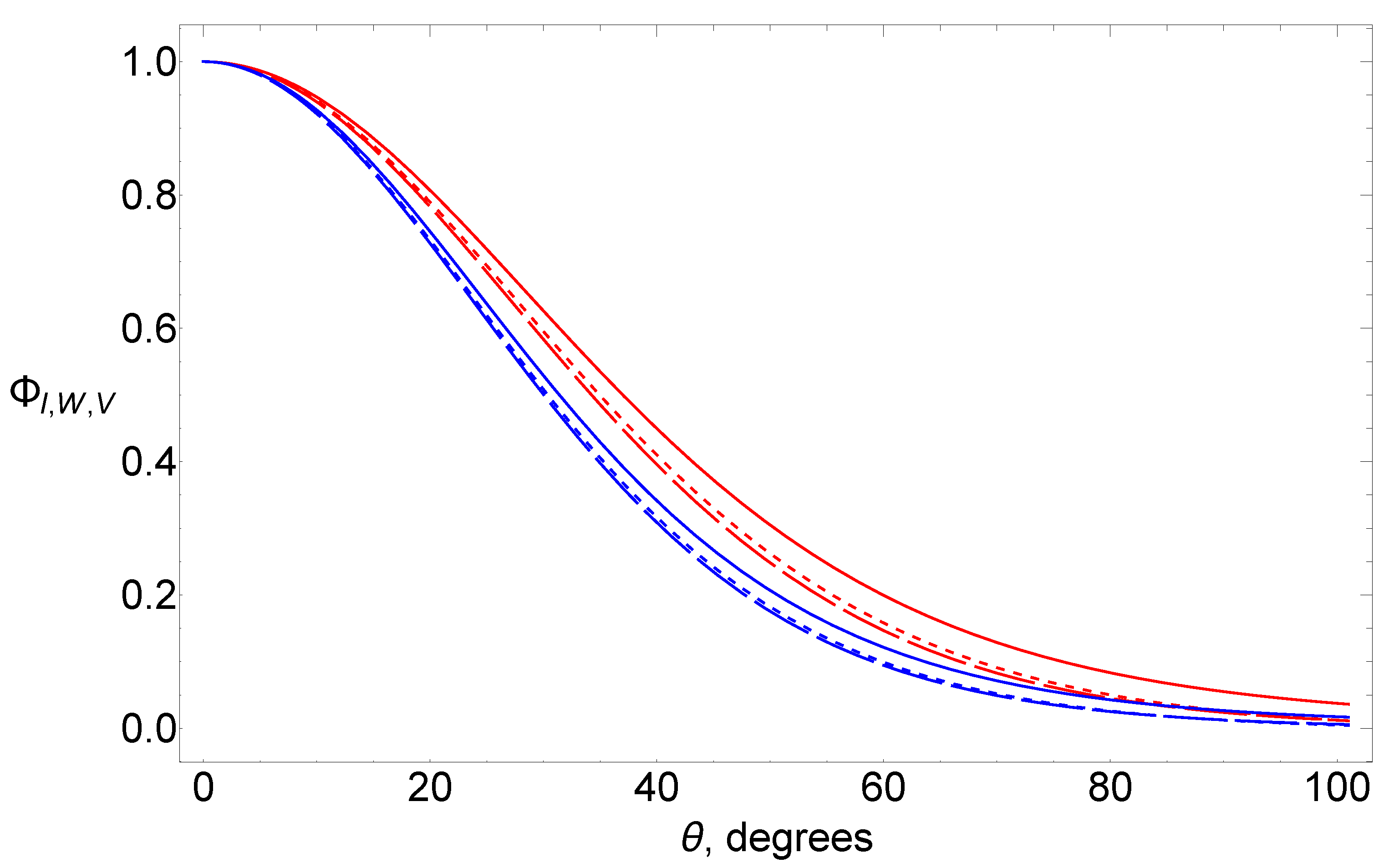
Figure 11.
Depolarization ratio as a function of dimensionless variables. Symbols (●—, ▪—,▴—) are the results of Monte Carlo simulations [17] for aqueous suspension of polystyrene spheres of diameter m (a,b) and m (c,d). Solid lines are the results of our calculations for (a,b) and (c,d).
Figure 11.
Depolarization ratio as a function of dimensionless variables. Symbols (●—, ▪—,▴—) are the results of Monte Carlo simulations [17] for aqueous suspension of polystyrene spheres of diameter m (a,b) and m (c,d). Solid lines are the results of our calculations for (a,b) and (c,d).


| sea water | ||
| 0.315 | 1.15 | |
| 0.313 | 1.12 | |
| aqueous suspension of polystyrene spheres | ||
| m | 0.383 | 1.17 |
| m | 0.294 | 1.23 |
Table 2.
The numerical values of and .
| sea water | ||||
| 0.49 | 0.645 | 0.47 | 0.610 | |
| 0.46 | 0.605 | 0.44 | 0.550 | |
| Henyey-Greenstein phase function/Rayleigh matrix | 0.47 | 1.50 | 0.38 | 1.50 |
| aqueous suspension of polystyrene spheres | ||||
| m | 0.46 | 1.38 | 0.10 | 1.38 |
| m | 0.40 | 1.57 | 0.34 | 1.57 |
© 2020 by the authors. Licensee MDPI, Basel, Switzerland. This article is an open access article distributed under the terms and conditions of the Creative Commons Attribution (CC BY) license (http://creativecommons.org/licenses/by/4.0/).
Share and Cite
MDPI and ACS Style
Gorodnichev, E.E.; Kondratiev, K.A.; Kuzovlev, A.I.; Rogozkin, D.B. Propagation and Depolarization of a Short Pulse of Light in Sea Water. J. Mar. Sci. Eng. 2020, 8, 371. https://doi.org/10.3390/jmse8050371
AMA Style
Gorodnichev EE, Kondratiev KA, Kuzovlev AI, Rogozkin DB. Propagation and Depolarization of a Short Pulse of Light in Sea Water. Journal of Marine Science and Engineering. 2020; 8(5):371. https://doi.org/10.3390/jmse8050371
Chicago/Turabian StyleGorodnichev, Evgeniy E., Kirill A. Kondratiev, Alexandr I. Kuzovlev, and Dmitrii B. Rogozkin. 2020. "Propagation and Depolarization of a Short Pulse of Light in Sea Water" Journal of Marine Science and Engineering 8, no. 5: 371. https://doi.org/10.3390/jmse8050371
Note that from the first issue of 2016, this journal uses article numbers instead of page numbers. See further details here.