Verification of Novel Maritime Route Extraction Using Kernel Density Estimation Analysis with Automatic Identification System Data

Abstract

A maritime route is used by sea transportation vessels to access the trading ports, and route design standards for the safety of maritime traffic have been established in various countries and organizations. However, no quantitative safety verification method related to route design currently exists. In this study, a novel maritime route was created and compared with the original route in Incheon, the Republic of Korea, based on the relevant automatic identification system (AIS) data. The attendant traffic density was revealed via kernel density estimation analysis of the AIS data, with the results used to create the boundary of the novel route through an image processing technique. The boundary and the centerline of the maritime route were determined using a line smoothing technique. For safety verification, the centerline of the original route and that of the novel maritime route were compared in terms of sinuosity, intersection angle, and route change envelope (RCE). The sinuosity analysis demonstrated that the route was stable in terms of the outer harbor limit, while the intersection angle analysis demonstrated that the novel maritime route intersection angle was stable. The RCE was used to objectively compare the absolute values of the distance change in the centerline.

1. Introduction

The shipping industry has witnessed rapid growth in the last three decades because of a significant increase in transportation demands [1]. In addition, as the vessel size continues to increase, countries and institutions around the world have been designing routes to prevent ship accidents and ensure safe shipping [2]. The passage used by sea transportation vessels for entering and exiting a trade port is known as a route. In the case of the Republic of Korea, the overall standards related to route design are determined according to the Harbor and Fishery Design Criteria. Here, the route width is determined to be 0.5–2.0 length overall, with some consideration of the ship’s length and the traffic conditions, while it is held as desirable that the radius of curvature does not exceed 30° in terms of the intersection angle of the bend [3]. The World Association for Waterborne Transport Infrastructure is a worldwide route design guideline centered on Europe [4]. According to this guideline, the route should be arranged as straight as possible, and the width design should be determined with some consideration of the interaction, natural phenomena, and fluid mechanic effects among the ships, while the curvature radius should be determined with taking the turning performance of the ship and the depth of the route into account [5].

As the vessels can cause serious problems when an accident occurs, such as loss of human life, damage to property, and environmental pollution, the route must be designed considering the characteristics of the vessel [6].

However, while numerous other countries have proposed similar route design standards, no method has been established to verify route stability quantitatively. Route stability is a method of quantitatively verifying that ships use a route safely. In terms of vessel operation, the greater the route width and smaller the intersection angle of the waypoint, the higher the route stability. Routes are designed only for coastal areas adjoining the ports; there are no routes in the sea far from land. Most vessels operate on recommended routes for the advantages of fuel efficiency and shortened distances; even if these routes do not exist, most ships traverse similar tracks [7].

In view of this, this study was initiated to devise various comparison methods based on actual data to verify the stability of the original route. The following study was referred to create a novel maritime route. The method of extracting the land road network as a means for creating a new route based on actual data was referenced. In the road network extraction method, detection, tracking, and image recognition technologies have been used. Here, we can include methods that use land vehicle data and crowdsourcing [8,9], research using the Global Positioning System (GPS) trajectory [10,11], and methods using satellite images [12,13]. In terms of marine networks, the route was extracted with reference to an existing study [14], where the maritime road network was extracted using the automatic identification system (AIS) data. The AIS data can be accessed in various ways, such as ship collision and grounding risk identification [15]. This study was based on the analysis of objects using roads and routes, as in the reference article, but performed a novel maritime route extraction based on the geographic information system (GIS). In addition, a new method was applied and analyzed to compare the designed route with the original route quantitatively. If the route stability of the novel maritime route, indicated by the vessel’s historical track, is better, it will be widely used in the maritime traffic field. In addition, the GIS and the actual data are used to analyze the relationship between ship accidents considering various ship characteristics [16]. This serves as the basic data to select the optimal route for MASS (Maritime Autonomous Surface Ship) through AIS data collection and processing [17]. The analysis area of the current study targets the original route’s coastal area for access to the Incheon Port in the Republic of Korea, while the AIS data includes latitude and longitude data in the form of GIS points [18]. Here, the AIS classification criteria were set to $\ge$ 200 m and $<$ 200 m. Vessels have different navigation patterns depending on their size, and the routes they use are also separated, especially in places where there are many vessels [19]. As described above, the analysis was classified into two setups in accordance with the trend of large-scale ships and changes to MASS. In addition, AIS data in the form of points were analyzed using the kernel density estimation (KDE) method, while various image processing techniques were used for the KDE analysis results. Following this, a centerline of the novel maritime route based on actual data was generated using line smoothing and Delaunay triangulation. The centerline of the novel maritime route thus generated compared the route safety with the centerline of the original route; this shows the efficiency index of route safety through various analyses. The final result is analyzed in terms of sinuosity, intersection angle, and route change envelope (RCE), with a focus on the safety verification of the existing routes.

2. Materials and Methods

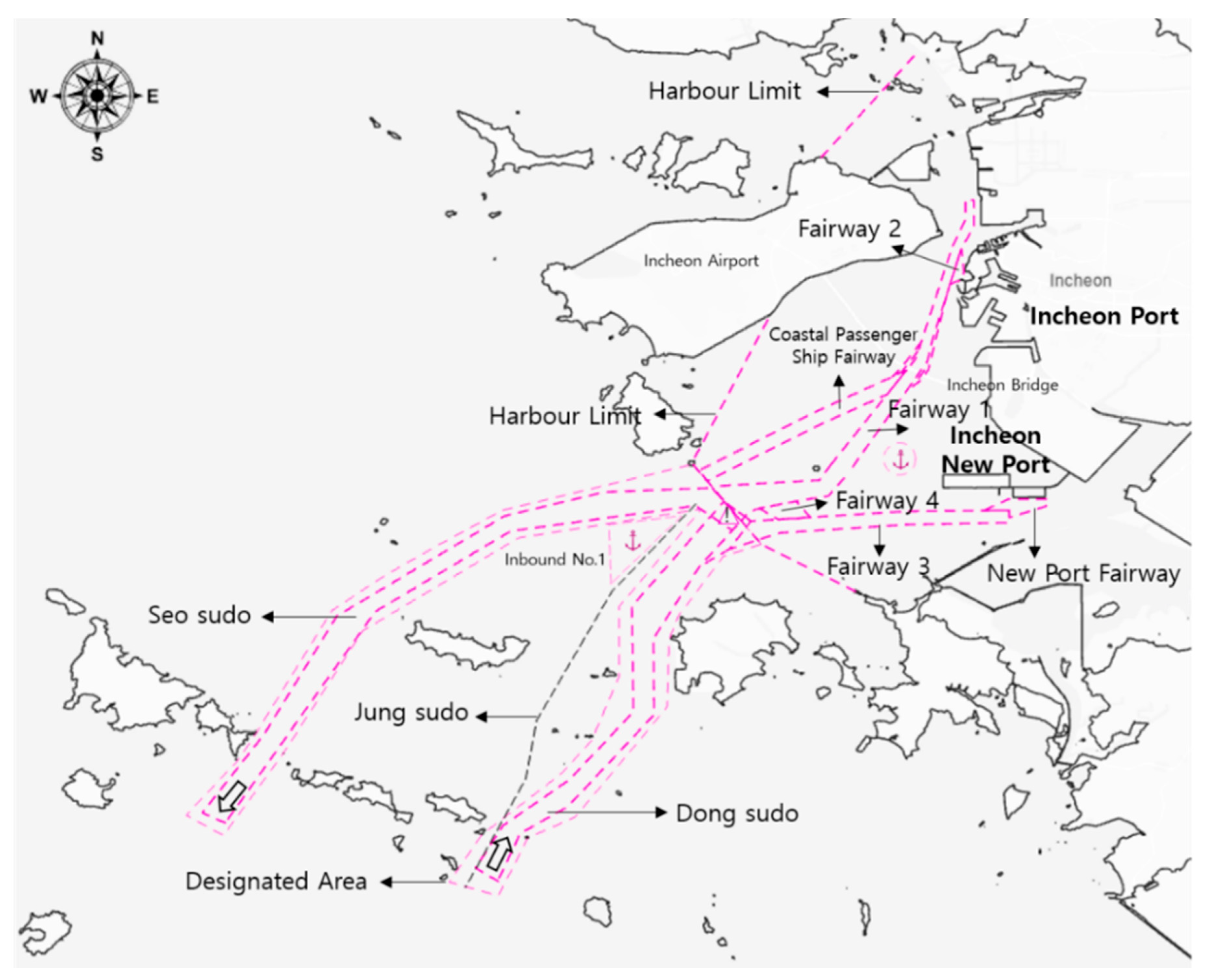
2.1. Analysis Area

This study was conducted on the coast of Incheon, the Republic of Korea. In Incheon Port, the routes are created based on the concept of harbor limit. This is divided into inner harbor limit and outer harbor limit, while the point where the routes meet is a sea area that requires attention due to the complicated maritime traffic involving various traffic flows. Figure 1 presents an overview of the area for analysis, the sea area of Incheon Port.

As Figure 1 shows, the outer harbor limit can be accessed through the inbound route, Dong sudo, using the Incheon New Port and Incheon Port. At the same time, the outbound routes include Seo sudo, the outbound route for small vessels, Jung sudo, and the Inbound No.1 anchorage. In terms of the inner harbor limit, there are 4 routes, Fairway 1 to Fairway 4, a coastal passenger ship fairway, and an anchorage.

2.2. AIS Data Characteristics

AIS technology provides a vast amount of near-real-time information, which calls for an ever-increasing degree of automation in transforming data into meaningful information to support operational decision makers [20].

Table 1. AIS data characteristics.

Categorization	AIS
Period	2019.03.01.–2020.02.29. (one year)
Analysis Area	Incheon, Republic of Korea
Ship Type	Passenger Ship (60–64, 69) Cargo Ship (70–74, 79) Tanker (80–84, 89)
Class 1	Under 200 m of Ship’s Type ($<200\mathrm{m})$
Class 2	200 m or Over of Ship’s Type ($\ge 200\mathrm{m}$)
Transmission Distance	50 Nautical Miles
Transmission Interval	2 s to 3 min

presents the characteristics of the AIS data.

As shown in Table 1, the data collection period was the 1-year period between 2019.03.01.–2020.02.29, while the data collection location was Incheon in the Republic of Korea. The collected AIS data included dynamic information such as position, date, and time, and static information, which included the Maritime Mobile Service Identity number, ship type, ship length, and ship beam [21]. The AIS data were extracted using the Marine Traffic and Safety Assessment Solution equipment [22]. In terms of the received AIS data, only passenger ships (60–64, 69), cargo ships (70–74, 79), and tankers (80–84, 89) using the routes were analyzed, and the traffic patterns varied depending on the size of the vessel. In view of this, 200 m was used as a reference point for large vessels, and Class 1 and Class 2 were used for all other vessels [23]. At the same time, the detection distance 50 nautical miles, and the transmission interval a minimum of 2 s and a maximum of 3 min depending on sailing conditions and vessel speed [24].

2.3. Novel Maritime Route Extraction Overview

In this study, we found that the stability of the novel maritime route was better compared with that of the original route. The process of collecting, processing, and analyzing the AIS data is shown in Figure 2.

Figure 2 presents an overview of the framework for creating a novel maritime route based on 1 year of the AIS data stored in the Amazon Web Services cloud server. First, data processing and plotting on GIS; we selected the analysis area for the study then converted them into World Geodetic System (WGS84) coordinates [25]. Next, we performed GIS-based density analysis and KDE analysis using the extracted AIS data. Second, route boundary extraction; image binarization, and image boundary extraction were used for this process. The image binarization used the Otsu method, and the boundary extraction used the canny method. Third, centerline extraction; the centerline was created using line smoothing and Delaunay triangulation. Finally, verification; we could draw conclusions in terms of the centerline and the sinuosity, intersection angle, and RCE of the existing route.

2.3.1. Summary of KDE

The collected AIS location information was based on WGS84, and we matched the coordinates to use the information in terms of the GIS. The data appeared as points in the form of vector data, which regarded the area as a continuous 2-dimensional space and made it is possible to generate points, lines, and polygons using a coordinate system. Furthermore, various forms of spatial analysis and density analysis were possible using raster data based on the grid cell concept.

Density analysis refers to a method of estimating the characteristics of random data variables. The most effective means for doing this involves drawing a histogram. A histogram is parametric and is suitable for visualizing only simple frequencies. However, such a method is discontinuous at the boundary of each bin and has different disadvantages depending on the width of the bin [26]. KDE is a method for estimating non-parametric density functions for data following non-parametric distributions. After generating the kernel function with a focus on the value of the data for each observed dataset, we could add all of the created kernel functions and then total them up before dividing this figure by the number of data [27]. Equation (1) is the equation for the kernel density estimation.

$$\widehat{f}\left(x,h\right)=\frac{1}{n}{\displaystyle \sum }_{i=1}^n{K}_h\left(x-x_i\right)$$

(1)

Here, $x$ is a random variable, and $x_i$ is observation. $h$ is bandwidth, kernel width, or smoothing parameter as a parameter for adjusting the kernel; the kurtosis of the kernel is determined according to the size of $h$. $K$ is divided by the sum of the observations with the kernel function applied to the total number of observations [28]. It is important to select an appropriate bandwidth for KDE because over-smoothing may occur in areas with high data density and under-smoothing may occur in areas with low data density. In short, the resulting bandwidth is a “free parameter” that greatly influences the estimations.

2.3.2. Calculating KDE Using the Geographic Information System

The predicted KDE at the $\left(x, y\right)$ position using the GIS can be determined using the following formula (Equation (2)).

$$D=\frac{1}{r^2}{\displaystyle \sum }_{i=1}^n\left[\frac{3}{\pi }\times p_i{(1-{\left(\frac{d_i}{r}\right)}^2)}^2\right]$$

(2)

Here, $D$ is the density calculation formula, $i$ is the number of points up to input size $n$, and $p_i$ is a number that can be applied with weights according to characteristics such as ship speed, ship length, and ship draft. Meanwhile, $d_i$ is the distance between point $i$ and the position $\left(x,y\right)$. In addition, $d_i$ must be less than $r,$ which represents the search radius [29]. Figure 3 shows an example to apply the kernel function around the point and to explain when the search radius is 500 m.

In this study, the KDE analysis using GIS data incorporated the quartic kernel [30]. The GIS program was provided only with the quartic kernel; the equation is as follows [31]:

$$K\left(\mu \right)=\frac{15}{16}{\left(1-{\mu }^2\right)}^2$$

(3)

Here, $\mu$ has the following condition ($\left|\mu \right|\le 1)$. That is, the kernel function was used for all the positions to estimate the density, with the results presented in the form of raster data. The raster data was input to the image processing step to create a route.

2.3.3. Image Processing

Road and route extraction techniques are generally classified into 6 categories: Basic image processing methods, frequency-based methods, knowledge-based approaches, supervised techniques, segmentation methods, and other methods [32]. In this study, a basic image processing method and a segmentation method were used. Here, binarization and edge extraction methods were used for the image processing method. This method was performed on the raster images generated via the KDE analysis. In addition, it refers to dividing the brightness of each pixel into light and dark areas based on a specific threshold value and then converting them into one brightness value [33]. By doing this method, the object contained in the image can be separated from the background. Here, the Otsu algorithm that incorporates a single threshold value, which is widely used as a binarization method, was used [34]. The image divided into black and white performs edge detection, which means the boundary of the route. Edge extraction methods are representative of Sobel, Laplacian, and Canny. In this study, the canny edge extraction method was used and was the most accurate method. The Canny algorithm uses a Gaussian filter to remove any noise and has a low error rate, with the position of the edge points measured as accurately as possible [35]. The Process of Canny edge detection algorithm can be broken down into 5 different steps; First, Apply a Gaussian filter to smooth the image in order to remove the noise. Since all edge detection results are easily affected by the noise in the image, it is essential to filter out the noise to prevent false detection caused by it. To smooth the image, a Gaussian filter kernel was convolved with the image. This step will slightly smooth the image to reduce the effects of obvious noise on the edge detector. For a Gaussian filter kernel of size $\left(2\mathrm{k}+1\right)\times \left(2\mathrm{k}+1\right)$, it can be expressed as Equation (4).

$$H_{ij}=\frac{1}{2\pi {\sigma }^2}exp\left(-\frac{{\left(i-\left(k+1\right)\right)}^2+{\left(j-\left(k+1\right)\right)}^2}{2{\sigma }^2}\right),1\le i,j\le \left(2k+1\right)$$

(4)

The following Equation (5) is a mask example of a 5 $\times$ 5 Gaussian filter used to create an adjacent image.

$$B=\frac{1}{159}\left[\begin{array}{ccc}2& 4& \begin{array}{ccc}5& 4& 2\end{array}\\ 4& 9& \begin{array}{ccc}12& 9& 4\end{array}\\ \begin{array}{c}5\\ 4\\ 2\end{array}& \begin{array}{c}12\\ 9\\ 4\end{array}& \begin{array}{c}\begin{array}{ccc}15& 12& 5\end{array}\\ \begin{array}{ccc}12& 9& 4\end{array}\\ \begin{array}{ccc}5& 4& 2\end{array}\end{array}\end{array}\right]$$

(5)

The localization error to detect the edge will slightly increase with the increase in the Gaussian filter kernel size. Mask 5 × 5 is a good size for most cases, but this will also vary depending on specific situations. Second, find the intensity gradients of the image. An edge in an image may point in a variety of directions, thus the canny algorithm uses 4 filters to detect horizontal, vertical, and diagonal edges in the blurred image. Third, apply non-maximum suppression to get rid of spurious response to edge detection. Fourth, apply a double threshold to determine potential edges. Finally, the detection of edges by suppressing all the other edges that are weak and not connected to strong edges.

2.3.4. Line Smoothing and Centerline Extraction

In the urban transportation plan of the land area, the nodes, links, paths, and networks of urban transportation are created based on the traffic volume. A node consists of various points, while the line connecting these nodes is known as a link. When these links are connected, they become paths, with the total set of paths known as a network [36]. In this study, the centerline was extracted based on the concepts of node and segment to create a novel maritime route based on maritime traffic.

The route created via the image processing technique consisted of raster data. That is, all the boundary images were in a jagged state, which is a form of a grid cell. This will result in low stability of the sinuosity and intersection angles taken into consideration during the creation of the route. A process of smoothing the boundary of the route created via the GIS-based KDE analysis was thus required, and this is shown in Figure 4. Figure 4a shows that the boundary of the route created by the image processing technique was grid-cell-based raster data, meaning that it was extracted as vector data polylines. Figure 4b shows the process of extracting the generated polyline vertices, while Figure 4c shows the process of removing the jagged part of the route and the part away from the route. This process involved removing any irregularly created areas and ship anchorages of density around the route to improve the accuracy. Figure 4d shows the line-smoothing operation, which involved smoothing the angled portion of the line data. The method for smoothing the line was determined in terms of quadratic interpolation. Here, interpolation refers to estimating a value located between known points from known values, while quadratic interpolation was used when 3 data points were provided. In this study, we used the polynomial approximation with an exponential kernel method, a technique for smoothing lines using approximation. Following this, a point was inserted inside the smoothly generated lines (Figure 4e). The spacing of the inserted points was set to 350 m, corresponding to the longest ship length that can enter Incheon Port.

Figure 5 shows the process of setting the classification value according to the number of individual triangles and neighboring triangles before subsequently creating the centerline.

In Figure 5a, the value of 1 indicates 1 neighboring triangle, the value of 2 indicates 2 neighboring triangles, and the value of 3 indicates 3 neighboring triangles. When the attributed values were entered for each triangle, they were classified according to the number of neighboring triangles. Based on this, the nodes required for the centerline and network creation could be created. The form produced through the Delaunay triangulation was a polygon shape (Figure 5b). When this form was divided into lines, and 50% of the points were formed as a percentage, both the center point and the center point constituting the curve could be created. Here, all the center points of the edges were removed. The nodes were created from triangles with values of between 1 and 3. The center point of the line starting from the triangle with a value of 1 was created as a node, while the median center point of the triangle with a value of 3 was also created as a node. As such, nodes, curves, and segments could be constructed to create a route centerline, with the lines connected with the corresponding elements.

3. Results

3.1. KDE and Density Results

In this study, KDE analysis was performed on the data classified as Class 1 and Class 2 in terms of ship length, and the conditions were as shown in

Table 2. Categorization of the KDE and density.

Categorization	KDE	Density
Data Format	$\left(x, y\right)$	$\left(x, y\right)$
Grid Cell	100 m	100 m
Search Radius	500 m	500 m
Out Cell Values	Densities	Densities
Method	Planar	Planar
Represent	90% of Total Traffic	90% of Total Traffic

below.

The KDE and density analyses were performed using the same data format. The size of the grid cell was set to 100 m, while the search radius from the random point was set to 500 m, to emulate the search radius of an artificial island, a maritime facility installed in the exclusive economic zone under Article 60, paragraph 5 of the United Nations Convention on the Law of the Sea. A radius of 500 m around the offshore structure was determined as the safety zone, and the standards for prohibiting access were applied [37]. Out cell values determine what the values in the output raster represent. There are two ways to do this, densities and expected counts. The values of densities are the output values that represent the predicted density value, whereas the expected counts values are the output values that represent the predicted amount of the phenomenon within each cell. As the cell value is linked to the specified cell size, the resulting raster cannot be resampled to different cell size and still represent the amount of the phenomenon. In terms of spatial analysis, the same analysis was performed using Planar. Finally, an area that accounts for more than 90% of maritime traffic for England and Belgium was selected as the route, and this was used for the maritime spatial planning (MSP) process. Here, the route was based on 90% of the total maritime traffic in terms of density [38,39]. Figure 6 shows how the data distribution was divided according to the number of quantiles. After dividing the maritime traffic data into 10 sections, 90% of the total traffic could be expressed, with the exception being the lower 0%–10% section. In the lower 0%–10% section, the detailed route cannot be extracted because all the tracks that the vessel has passed even once were marked in the GIS environment.

As such, KDE and density analyses were performed in terms of Class 1 and Class 2.

Table 3. Analysis results KDE and density for class 1.

No.	Percentage	Color	KDE	Density
1	0%–10%	None	$\le$ 1234051.0	$\le$ 3137150.2
2	10%–20%		$\le$2468102.5	$\le$6274300.5
3	20%–30%		$\le$4936205.0	$\le$9411450.7
4	30%–40%		$\le$7404307.5	$\le$15685751.2
5	40%–50%		$\le$11106461.3	$\le$21960051.7
6	50%–60%		$\le$16042666.4	$\le$31371502.4
7	60%–70%		$\le$23446973.9	$\le$43920103.4
8	70%–80%		$\le$33319384.0	$\le$56468704.3
9	80%–90%		$\le$45659896.7	$\le$72154455.6
10	90%–100%		$\le$314683072.0	$\le$799973312.0

shows the results of the Class 1 analysis, with the visualizations shown in Figure 7.

Figure 7a shows the result of the KDE analysis, and Figure 7b shows the results using density analysis. In Figure 7b, we found that the density analyzed route was cut off in some sections. In addition, it can be seen that the width of the route was narrower than that obtained using the KDE result. Meanwhile,

Table 4. Analysis results from KDE and density for Class 2.

No.	Percentage	Color	KDE	Density
1	0%–10%	None	$\le$164983.1	$\le$301385.6
2	10%–20%		$\le$494949.3	$\le$904156.9
3	20%–30%		$\le$1154881.7	$\le$1808313.8
4	30%–40%		$\le$2144780.3	$\le$3013856.3
5	40%–50%		$\le$3646645.2	$\le$4520784.4
6	50%–60%		$\le$4949493.1	$\le$6329098.2
7	60%–70%		$\le$6269358.0	$\le$8137412.0
8	70%–80%		$\le$7754205.9	$\le$10247111.4
9	80%–90%		$\le$9239053.9	$\le$12658196.5
10	90%–100%		$\le$42070692.0	$\le$76853336.0

shows the results of the Class 2 analysis, with the visualizations shown in Figure 8.

Figure 8a shows the result of the KDE analysis, and Figure 8b shows the results using density analysis. From Figure 7 and Figure 8, we found that some sections of the density analysis were cut off when compared with the original route, which was not suitable for the creation of a novel maritime route. Moreover, it can be seen that the density legend has an interval twice as wide as the KDE legend.

Furthermore, using the same conditions for the Class 1 and Class 2 KDE and density analyses, when analyzing the density of the bins according to the legends, the bin boundaries were not smooth when visualized. Therefore, an image processing technique was subsequently used for further analysis.

3.2. Novel Maritime Route Binarization

The novel maritime route binarization was performed on the KDE results of Class 1 and Class 2. These binarized images were used to detect the characteristics of the included route and were the basic operation for use in route stability applications. The images can represent only the route part, as shown in Figure 9.

Figure 9 shows the results of the Class 1 and Class 2 binarization using the Otsu algorithm. The route area was represented by the dark area, with the other areas represented by the light areas.

3.3. Novel Maritime Route Boundary Extraction

It can be seen that the extracted binarization images present a contrast of black and white. However, the boundary was extracted to ascertain the edge value of the route. To extract the boundary from the image, after differentiating the image, we identified the portion with a derivative value greater than a specific threshold. The following paragraphs outline the Canny of edge extraction algorithm. Figure 10 shows the canny results of the edge extraction analysis.

The Canny algorithm is capable of extracting more precise edges due to noise filtering. The noise filtering canny method makes it possible to extract the edge of an accurate route in a GIS environment.

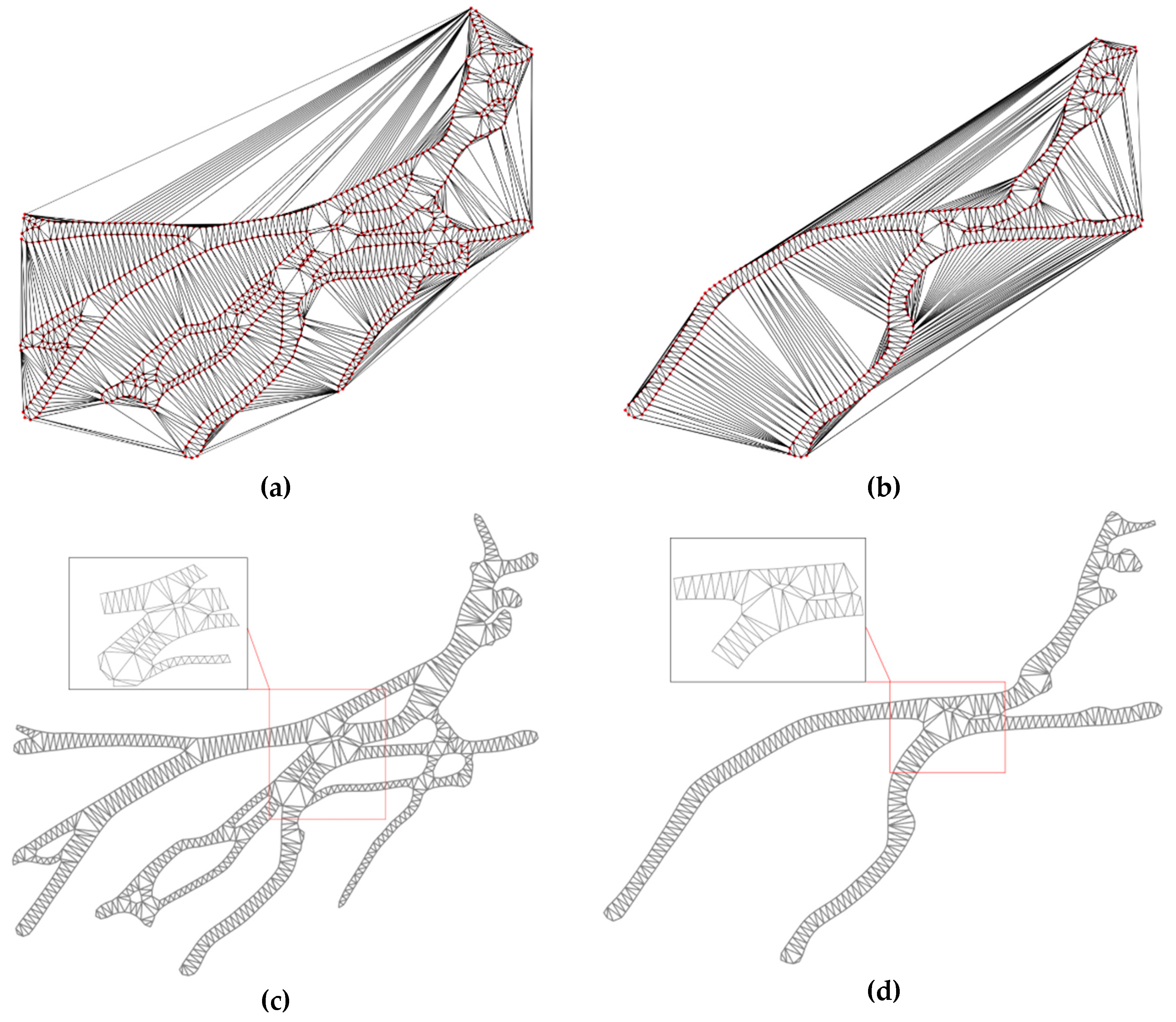
3.4. Line smoothing and Delaunay triangulation result

The result of extracting the route boundary performed line smoothing. The jagged boundary was removed to create an improved route than the original route. The smoothed line was inserted with points at regular intervals to proceed to the next process; the Delaunay triangulation was performed by inserting points at regular intervals. Delaunay triangulation involves creating and dividing triangles in a way that they do not contain points other than those used when creating the triangles on the points on the plane. One of the most important features of the Delaunay triangulation is that “the circumscribed circle of any triangle does not contain any point other than the three vertices of that triangle.” This feature is useful for data clustering, density analysis, and road network design as it can identify the closest point [40]. Figure 11 shows the results of the Delaunay triangulation in terms of Class 1 and Class 2. The initial appearances after applying the Delaunay triangulation are shown in Figure 11a,b, while Figure 11c,d show the results after filtering out all the parts that were not routes.

3.5. Novel Maritime Centerline Generation

The Delaunay triangulation results can be used as input in terms of the values attributed according to the number of triangles that share the faces of neighboring edges to create the centerline of the route. The final centerline is shown in Figure 12.

Figure 12a shows the centerline of Class 1, while Figure 12b shows the centerline of Class 2 and defines it as a novel maritime centerline. The centerline of the original route was created by connecting the center points of the edges and then comparing this with the novel maritime centerline.

4. Discussion

4.1. Verification of Sinuosity

In this study, the sinuosity ($\overline{S}$) was compared and analyzed in terms of the novel maritime centerline and the original route centerline to verify the route safety. The routes used for comparison were Fairway 1, Dong sudo, and Seo sudo. The coastal passenger fairways 2–4 were excluded because they presented straight lines, which were unsuitable for sinuosity comparisons. The sinuosity route was used as an index indicating the bend, which can be expressed in terms of Equation (6).

$$\overline{S}=\frac{L_c}{L_s}$$

(6)

The description of $\overline{S}$ is equal to the following fraction. $L_s$ is the denominator for the length of straight fairway distance, and $L_c$ is the length of the centerline is the numerator. This value means that the closer to the value of 1, the closer the straight line. Therefore, the $\overline{S}$ value of the original centerline and the $\overline{S}$ value of the novel maritime centerline can be obtained, and the difference between these $\overline{S}$ values are multiplied by 100 to obtain $∆\overline{S}.$ Figure 13 presents an overview of the comparison between the centerline of the original route and that of the novel maritime route in terms of the Seo sudo, Dong sudo, and Fairway 1 routes. In addition, there are many routes in the Incheon Port, but the length of the route is short and simple. Therefore, it was not analyzed in this study.

Table 5. Differences among straight line, centerline, and sinuosity.

Area	Category	Centerline of Original Route	Centerline of Class 1	Centerline of Class 2
Seo sudo	$L_s$	32.42 km
	$L_c$	34.84 km	35.09 km	34.71 km
	Difference	+2.42 km	+2.67 km	+2.29 km
	$\overline{S}$	1.074	1.082	1.070
	$∆\overline{S}$	-	+0.8	−0.4
Dong sudo	$L_s$	25.94 km
	$L_c$	27.00 km	27.58 km	26.36 km
	Difference	+1.06 km	+1.64 km	+0.42 km
	$\overline{S}$	1.041	1.063	1.016
	$∆\overline{S}$	-	+2.2	−2.5
Fairway 1	$L_s$	18.12 km
	$L_c$	18.38 km	20.08 km	19.33 km
	Difference	+0.26 km	+1.96 km	+1.21 km
	$\overline{S}$	1.014	1.108	1.066
	$∆\overline{S}$	-	+9.4	+5.2

shows the distance difference between the straight line and the centerline of the routes used for the analysis. Here, the smaller the value, the closer the straight line. The graph in Figure 14a presents a comparison of the distance between the analyzed route and the sinuosity, while Figure 14b presents a graphical representation of the resulting values. The small Class 1 vessels returned large flexural results in terms of Seo sudo (+0.8) and Dong sudo (+2.2), while the large Class 2 vessels demonstrated small curvatures with Seo sudo (–0.4) and Dong sudo (–2.5). The Class 1 vessels exhibited various movements at sea, meaning the shape of the centerline was complicated. At the same time, since the Class 2 vessels had a simple historical track and simple inbound/outbound routes due to the limitations of vessel operation, the sinuosity was small. In terms of Fairway 1, the sinuosity for Class 1 was +9.4 and that for Class 2 was +5.2, which indicates a large degree of curvature. For that reason, the centerline that enters and departs from the northern, central, and southern parts of Incheon Port returned large results due to the creation of operated passenger ship and small vessels. In addition, Fairway 1 is shorter than Dong sudo and Seo sudo and has the closest shape. Based on this, it can be stated that the longer the route and the fewer ports in the vicinity, the better the effect. The sinuosity was not close to a straight line, while the fewer the nearby ports, the better the stability of the novel maritime centerline. However, limitations were found in the adjacent areas of the port.

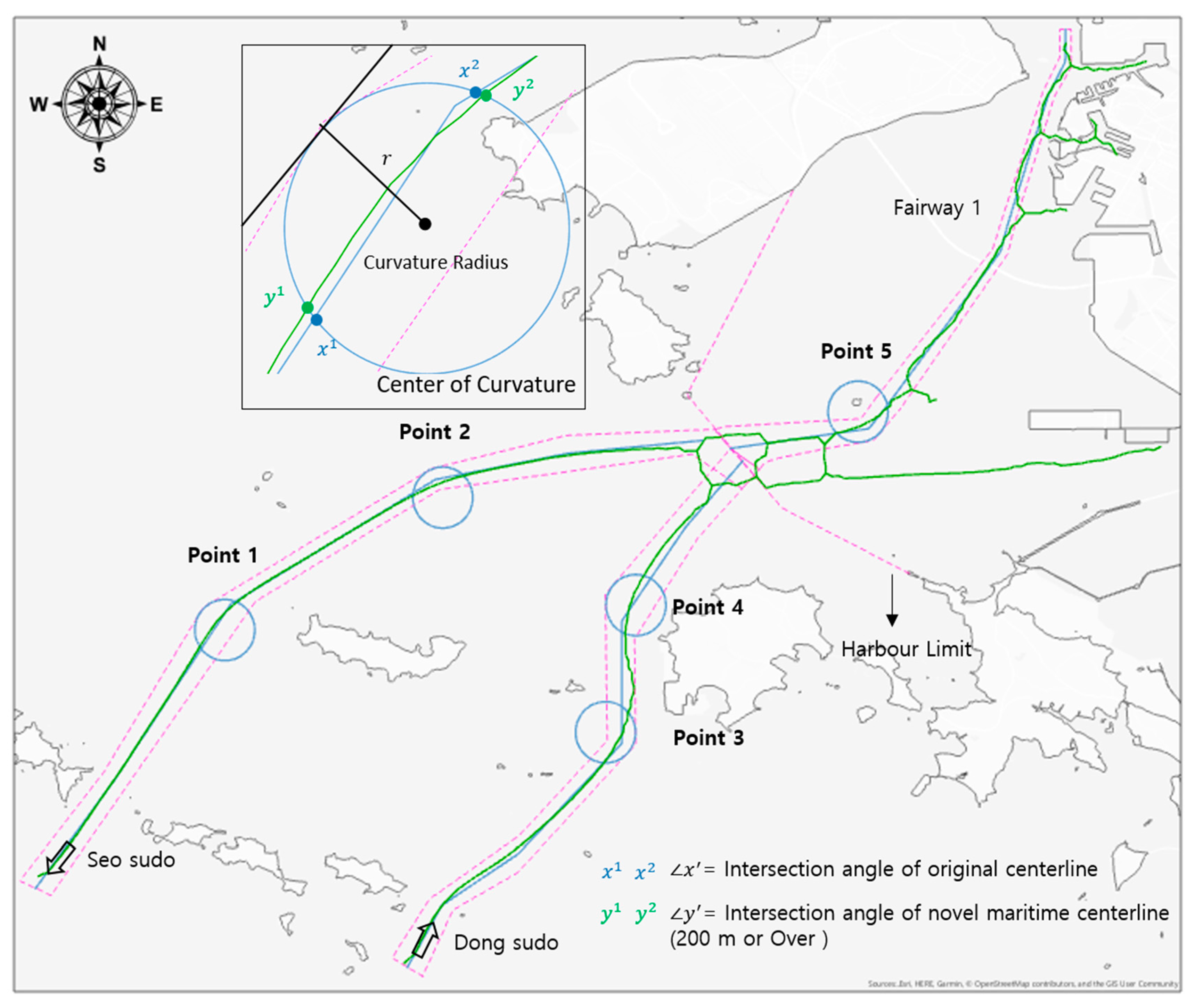
4.2. Verification of Intersection Angle

The intersection angle point is the waypoint of the vessel when turning, and the curvature with a radius r allowed us to analyze the intersection angle of the original route centerline, $\angle x^1{x}^2$, and that of the novel maritime route centerline, $\angle y^1{y}^2$. As a singularity, Point 5 is a route that includes both inbound and outbound traffic, and was thus analyzed separately. Using Equation (7), we verified whether the reduction rate of the novel maritime route $\overline{∆\mathrm{R}}$ was quantitatively efficient according to the intersection results as.

$$\overline{∆\mathrm{R}}=\frac{\angle x^{\prime }-\angle y^{’}}{\angle x^{\prime }}\times 100$$

(7)

Equation (6) represents the reduction rate of the novel maritime route. Here, $\angle x^{\prime }$ is the intersection angle of the original centerline as a numerator, $\angle y^{\prime }$ is the intersection angle of novel maritime centerline as a denominator, which is expressed as a percentage. The intersection angle of the novel maritime route centerline and that of the original route centerline were compared and analyzed in terms of the five largest turning angles in the Incheon coastal area. The intersection angle is the angle formed by two straight lines when they meet. Five intersection angle points were selected for analysis and labeled points 1 to 5. This included two points in Seo sudo, two in Dong sudo, and one in Fairway 1. The locations are shown in Figure 15.

The results of the intersection angle analysis are shown in

Table 6. Difference in intersection angle between the original route and the novel maritime route.

Area	Intersection Angle of Original Route	Class 1		Class 2
		Angle	$\mathbf{∆}\mathbf{R}$	Angle	$\mathbf{∆}\mathbf{R}$
Point 1	25°	16.3°	8.7° (34.8%)	11.3°	13.7° (54.8%)
Point 2	20°	21.8°	−1.8° (−9.0%)	7.6°	12.4° (62.0%)
Point 3	37°	19.7°	17.3° (46.7%)	15.2°	21.8° (58.9%)
Point 4	35°	10.8°	24.2° (69.1%)	13.7°	21.3° (60.8%)
Point 5	IN 48°	17.2°	30.8° (64.2%)	16.0°	32.0° (66.6%)
	OUT 53°	23.9°	29.1° (54.9%)	20.6°	32.4° (61.1%)

and Figure 16. As Table 6 shows, the intersection angle of the original route appears from a minimum of 20° to a maximum of 53°. This value is the route created by the route design method of the Republic of Korea. Points 1 to 5 are points for turning the vessel, and the lower the intersection angle value, the higher the stability of the route. As a result of the analysis, vessels using this original route actually make different intersection angles. The intersection angle of Class 1 ranges from a minimum of 10.8° to a maximum of 23.9°. The value of $∆\mathrm{R}$, the reduction rate, showed that the intersection angle of the novel maritime route was high, except for the value of point 2. The reason for the larger intersection angle value of −9.0% for point 2 is that there are vessels entering and leaving in different directions. The intersection angle of Class 2 ranges from a minimum of 12.4° to a maximum of 32.4°. It was found that the value of the reduction rate r decreased from 54.8% to 66.6%. Class 2 showed that the intersection angles of the novel maritime route were all highly stable. Figure 16a presents a graphical representation of the intersection angles of the five points, and Figure 16b presents the reduction rate of the intersection angles. The reason why Point 2 of Class 1 had larger results is that a number of small ships and passenger ships do not pass to the end of Seo sudo. In the case of Class 2, small intersection results were observed, indicating the value was changed as a result of the passing patterns that depended on the size of the ship. In terms of intersection angle, the novel maritime centerlines showed more stable results, with the exception of one region.

4.3. Verification of RCE

The RCE value sets the original centerline as the baseline and indicates the distance between the novel maritime centerlines. This value involves only the total distance traveled as an absolute value based on the observation point, regardless of time, and always has a positive value. The RCE value is considered to be a useful indicator in terms of route stability based on the distance from the baseline. Figure 17 shows an overview of the RCE analysis.

Figure 18 shows the RCE values of the centerlines used in the analysis. In terms of Class 1, the RCE value was 137.57 m for Seo sudo, 106.77 m for Dong sudo, and 226.12 m for Fairway 1. Meanwhile, in terms of Class 2, the RCE value was 59.66 m for Seo sudo, 152.09 m for Dong sudo, and 108.05 m for Fairway 1. Class 1 has a large RCE from the original centerline due to the influence of ships operating in various places. In Dong sudo, the distance between Class 2 vessels was 152.09 m, meaning the largest RCE was in the middle area of the Dong sudo and safe operation was thus crucial in this area. In the case of Fairway 1, the RCE was large due to the various routes entering Incheon Port. As such, the location where the RCE value was large was one where the distance between the centerlines was large, meaning it was important to review the navigational conditions and the safety of the route. In addition, when the route was divided into detail, there were a total of 4 RCE values of 200 m or more, which is a standard for a large vessel. Although the conditions of the ship’s operation and various conditions of the sea should be considered, the place where the RCE value was high is a section to be careful because the traffic of the ship is complicated. This section of the state requires safe operation for both the country and the agency designing the route and for the ship operator.

5. Conclusions

Route design is very important to ensure the safe navigation of large vessels, and it is necessary to verify the route stability. To verify the stability of a newly designed maritime route in quantitative terms, we extracted, compared, and analyzed the new routes based on actual data. KDE analysis was applied in terms of AIS data density analysis, with the results undergoing binarization and boundary extraction using an image processing technique. The novel maritime route and its centerline were created using line boundary smoothing and Delaunay triangulation. Following this, sinuosity, intersection angle, and RCE were analyzed for verification of the safety of the novel maritime centerline compared with that of the original centerline.

In general, the route stability of novel maritime routes was superior to the original route. However, there are limitations; the novel maritime route generation technique will be reviewed in the areas where the route is newly established with the existing route design criteria. In addition, all these processes involved GIS and Python rather than a single program, and the analysis area was limited to the Incheon coast. In view of this, future work should involve one uniform program, while the route should be created based on the AIS data of ships operating in all the sea areas of Korea, not only the Incheon coastal area. Finally, we should further investigate the advanced research conducted overseas using ship AIS data to create routes via various analytical techniques. This will involve studying the criteria reflected in the navigation area of the MSP process and applying it to the shortest distance and the optimal route selection of autonomous ships using maritime-based centerlines and networks.

References

1. Jinxian, W.; Dong, Y. Investigation of shipping accident injury severity and mortality. Accid. Anal. Prev. 2015, 76, 92–101. [Google Scholar]
2. Debnath, A.K.; Chin, H.C. Navigational traffic conflict technique: A proactive approach to quantitative measurement of collision risks in port waters. J. Navig. 2010, 63, 137–152. [Google Scholar] [CrossRef] [Green Version]
3. MOF (Ministry of Oceans and Fisheries). Harbour and Fishery Design Criteria; MOF: Sejong, Korea, 2017. [Google Scholar]
4. Park, J.M. A Study on the Establishing Methods of Design Criteria of Inland Waterways in Korea. Master’s Thesis, Korea Maritime and Ocean University, Busan, Korea, 2011. [Google Scholar]
5. PIANC (The world Association for Waterborne Transport Infrastructure). MarCom Working Group 121: Harbour Approach Channels—Design Guidelines; PIANC: Brussels, Belgium, 2014. [Google Scholar]
6. Akten, N. Analysis of shipping casualties in the Bosphorus. J. Navig. 2004, 57, 345–356. [Google Scholar] [CrossRef]
7. Robert, E.G.; Jarno, S.; Laura, R.; Heidi, K.; Floris, G.; Jakub, M.; Robin, B.; Ville, K. A method for ice-aware maritime route optimization. In Proceedings of the 2014 IEEE/ION Position, Location and Navigation Symposium—PLANS 2014, Monterey, CA, USA, 5–8 May 2014; pp. 1371–1378. [Google Scholar]
8. Wei, Y.; Ai, T.; Wei, L. A method for extracting road boundary information from crowdsourcing vehicle GPS trajectories. Sensors 2018, 18, 1261. [Google Scholar]
9. Zuchao, W.; Tangzhi, Y.; Min, L.; Xiaoru, Y.; Huamin, Q.; Jacky, Y.; Qianling, W. Visual exploration of sparse traffic trajectory data. IEEE Trans. Vis. Comput. Graph. 2014, 20, 1813–1821. [Google Scholar]
10. James, B.; Jakob, E. Inferring road maps from global positioning system traces. J. Transp. Res. Board 2012, 2291, 61–71. [Google Scholar]
11. Xuemei, L.; Yin, W.; James, B.; Jakob, E.; Yamin, Z. Mining large-scale, sparse GPS traces for map inference: Comparison of approaches. In Proceedings of the 18th ACM SIGKDD international conference on Knowledge discovery and data mining, New York, NY, USA, 12–16 August 2012; pp. 669–677. [Google Scholar]
12. Mohamad, T.; Azriel, R. Building and road extraction from aerial photographs. IEEE Trans. Sys. Man Cybern. 1982, 12, 84–91. [Google Scholar]
13. Volodymyr, M.; Geoffrey, E.H. Learning to Detect Roads in High-Resolution Aerial Images; University of Toronto: Toronto, ON, Canada, 2010; pp. 210–223. [Google Scholar]
14. Guiling, W.; Jinlong, M.; Yanbo, H. Extraction of maritime road networks from large-scale AIS data. IEEE Access 2019, 7, 123035–123048. [Google Scholar]
15. Azzeddine, B.; Ingrid, K.G.; Erik, V.; Oystein, E. AIS-Based Multiple Vessel Collision and Grounding Risk Identification based on Adaptive Safety Domain. J. Mar. Sci. Eng. 2020, 8, 5. [Google Scholar]
16. Liye, Z.; Qiang, M.; Tien, F.F. Bing AIS data based spatial-temporal analyses of ship traffic in Singapore port waters. Transport. Res. Part E 2017, 129, 287–304. [Google Scholar]
17. Xinyu, Z.; Chengbo, W.; Yuanchang, L.; Xiang, C. Decision-Making for the Autonomous Navigation of Maritime Autonomous Surface Ships Based on Scene Division and Deep Reinforcement Learning. Sensors 2019, 19, 4055. [Google Scholar]
18. Lee, J.S.; Son, W.J.; Lee, B.K.; Cho, I.S. Optimal site selection of floating offshore wind farm using genetic algorithm. J. Korean Soc. Mar. Environ. Saf. 2019, 25, 658–665. [Google Scholar] [CrossRef]
19. MPA (Maritime and Port Authority of Singapore). Safety of Navigation in the Singapore Strait; MPA: Singapore, 2006. [Google Scholar]
20. Tixrant, M.L.; Guyader, D.L.; Gourmelon, F.; Queffelec, B. How can Automatic Identification System (AIS) data be used for maritime spatial planning. Ocean Coastal Manag. 2018, 166, 18–29. [Google Scholar] [CrossRef] [Green Version]
21. Giuliana, P.; Michele, V.; Karna, B. Vessel Pattern Knowledge Discovery from AIS data: A framework for anomaly detection and route prediction. Entropy 2013, 15, 2218–2245. [Google Scholar]
22. Lee, B.K.; Cho, I.S.; Kim, D.H. A study on the design of the grid-cell assessment system for the optimal location of offshore wind farms. J. Korean Soc. Mar. Environ. Saf. 2018, 24, 848–857. [Google Scholar] [CrossRef]
23. National Law Information Center. Maritime Safety Act; Republic of Korea. Available online: http://www.law.go.kr/ (accessed on 27 March 2020).
24. Lee, M.K.; Park, Y.S. Collision prevention algorithm for fishing vessels using mmWAVE communication. J. Mar. Sci. Eng. 2020, 8, 115. [Google Scholar] [CrossRef] [Green Version]
25. Lee, J.S.; Son, W.J.; Lee, H.T.; Cho, I.S. A Study on the Factors Affecting Optimal Site of Offshore Wind Farm from the Perspective of Maritime Traffic using Spatial Analysis. J. Korean Coastal Disaster Prev. 2020, 7, 85–96. [Google Scholar] [CrossRef]
26. Botev, Z.I.; Grotowski, J.F.; Kroese, D.P. Kernel density estimation via diffusion. Ann. Stat. 2010, 38, 2916–2917. [Google Scholar] [CrossRef] [Green Version]
27. Cho, H.J. Initialization Method of Model-Based Clustering Using Kernel Density Estimation: Using Big Data of Corporate Default. Master’s Thesis, Kookmin University, Seoul, Korea, 2017. [Google Scholar]
28. Alexander, B.; Carl, J.; Ylva, R. Modeling Bivariate Distributions Using Kernel Density Estimation. In Project in Computational Science; Uppsala University: Uppsala, Sweden, 2016; pp. 1–48. [Google Scholar]
29. Esri. How Kernel Density Works. Available online: https://pro.arcgis.com/en/pro-app/tool-reference/spatial-analyst/how-kernel-density-works.htm (accessed on 27 March 2020).
30. Silverman, B.W. Density Estimation for Statistics and Data Analysis. In Monographs on Statistics and Applied Probability; Chapman and Hall: London, UK, 1986; pp. 120–158. [Google Scholar]
31. Nicolas, L.; Xavier, W. Fast and stable multivariate kernel density estimation by fast sum updating. J. Comput. Graph. Stat. 2019, 28, 596–608. [Google Scholar]
32. Pramod, K.S.; Navin, R.; Rajesh, M. A comparison of road network extraction from High Resolution Images. In Proceedings of the First International Conference on Secure Cyber Computing and Communication, Jalandhar, India, 15–17 December 2018; pp. 525–531. [Google Scholar]
33. Kim, J.H.; Kim, G.B. A Binarization Technique using Histogram Matching for License Plate with a Shadow. J. Broadcast Eng. 2014, 19, 56–63. [Google Scholar] [CrossRef] [Green Version]
34. Otsu, N. A Threshold Selection Method from Gray-Level Histograms. IEEE. Trans. Sys. Man. Cybern. 1979, 9, 62–66. [Google Scholar] [CrossRef] [Green Version]
35. Canny, J. A Computational Approach to Edge Detection. IEEE Trans. Pattern Anal. Mach. Intell. 1987, 8, 184–203. [Google Scholar]
36. Park, C.S.; Kwon, Y.S. Urban Traffic Engineering; Book publishing kkubeog: Seoul, Korea; pp. 330–346.
37. UN (United Nations). United Nations Convention on the Law of the Sea; UNCLOS: New York, NY, USA, 1982; p. 45. [Google Scholar]
38. MCA (Maritime and Coastguard Agency). MGN 543(M+F) Safety of Navigation: Offshore Renewable Energy Installations (ORELs), Guidance on UK Navigation Practice, Safety and Emergency Response; MCA: Southampton, UK, 2016; p. 18. [Google Scholar]
39. Marine Spatial Plan for the Belgian part of the North Sea; Brussels, Belgium, 2016; pp. 42–43.
40. Lee, D.T.; Schachter, B.J. Two algorithms for constructing a Delaunay triangulation. Int. J. Comput. Inf. Sci. 1980, 9, 219–242. [Google Scholar] [CrossRef]
Figure 1. Overview of the area for analysis.
Jmse 08 00375 g001
Figure 2. Flowchart of the novel maritime route extraction process.
Jmse 08 00375 g002
Figure 3. How the kernel function is applied inside the search radius: (a) An example of applying the kernel function to the sample point and search radius; (b) an example of applying the kernel function when the four points and the search radius are all 500 m.
Jmse 08 00375 g003
Figure 4. Overview of the boundary smoothing process: (a) boundary of the route created by the image processing; (b) extraction of polyline vertices; (c) removing the jagged part; (d) line-smoothing operation; (e) inserted point inside the smoothly lines.
Jmse 08 00375 g004
Figure 5. (a) Inserting the attributed values according to the number of neighboring triangles; (b) organization of the nodes, curves, and segments to create the centerlines.
Jmse 08 00375 g005
Figure 6. Division of maritime traffic into 10 categories using the quantile method.
Jmse 08 00375 g006
Figure 7. Results of Class 1 analysis, with the exclusion of the 0%–10% data: (a) KDE analysis; (b) density analysis.
Jmse 08 00375 g007
Figure 8. Results of Class 2 analysis, with the exclusion of the 0%–10% data: (a) KDE analysis; (b) density analysis.
Jmse 08 00375 g008
Figure 9. Binarization results using the Otsu algorithm: (a) Class 1; (b) Class 2.
Jmse 08 00375 g009
Figure 10. Results of the boundary extraction using an edge extraction algorithm: (a) Canny algorithm Class 1; and (b) Canny algorithm Class 2.
Jmse 08 00375 g010
Figure 11. Delaunay triangulation results: (a), (b) Before filtering (Class 1 and Class 2); (c), (d) after filtering (Class 1 and Class 2).
Jmse 08 00375 g011
Figure 12. Centerline created through connecting nodes and curves: (a) Class 1 centerline creation; (b) Class 2 centerline creation.
Jmse 08 00375 g012
Figure 13. Overview of sinuosity analysis.
Jmse 08 00375 g013
Figure 14. Sinuosity distance and index results: (a) Between straight line and centerline; (b) comparison of sinuosity.
Jmse 08 00375 g014
Figure 15. Overview of the intersection angle analysis.
Jmse 08 00375 g015
Figure 16. Intersection angle results: (a) Comparison of intersection angles; (b) reduction rate of intersection angles.
Jmse 08 00375 g016
Figure 17. Overview of the route change envelope (RCE) analysis.
Jmse 08 00375 g017
Figure 18. RCE results: (a) Seo sudo; (b) Dong sudo; and (c) Fairway 1.
Jmse 08 00375 g018