3D Multiple Sound Source Localization by Proposed Cuboids Nested Microphone Array in Combination with Adaptive Wavelet-Based Subband GEVD

Abstract

Sound source localization is one of the applicable areas in speech signal processing. The main challenge appears when the aim is a simultaneous multiple sound source localization from overlapped speech signals with an unknown number of speakers. Therefore, a method able to estimate the number of speakers, along with the speaker’s location, and with high accuracy is required in real-time conditions. The spatial aliasing is an undesirable effect of the use of microphone arrays, which decreases the accuracy of localization algorithms in noisy and reverberant conditions. In this article, a cuboids nested microphone array (CuNMA) is first proposed for eliminating the spatial aliasing. The CuNMA is designed to receive the speech signal of all speakers in different directions. In addition, the inter-microphone distance is adjusted for considering enough microphone pairs for each subarray, which prepares appropriate information for 3D sound source localization. Subsequently, a speech spectral estimation method is considered for evaluating the speech spectrum components. The suitable spectrum components are selected and the undesirable components are denied in the localization process. The speech information is different in frequency bands. Therefore, the adaptive wavelet transform is used for subband processing in the proposed algorithm. The generalized eigenvalue decomposition (GEVD) method is implemented in sub-bands on all nested microphone pairs, and the probability density function (PDF) is calculated for estimating the direction of arrival (DOA) in different sub-bands and continuing frames. The proper PDFs are selected by thresholding on the standard deviation (SD) of the estimated DOAs and the rest are eliminated. This process is repeated on time frames to extract the best DOAs. Finally, K-means clustering and silhouette criteria are considered for DOAs classification in order to estimate the number of clusters (speakers) and the related DOAs. All DOAs in each cluster are intersected for estimating the position of the 3D speakers. The closest point to all DOA planes is selected as a speaker position. The proposed method is compared with a hierarchical grid (HiGRID), perpendicular cross-spectra fusion (PCSF), time-frequency wise spatial spectrum clustering (TF-wise SSC), and spectral source model-deep neural network (SSM-DNN) algorithms based on the accuracy and computational complexity of real and simulated data in noisy and reverberant conditions. The results show the superiority of the proposed method in comparison with other previous works.

1. Introduction

Sound source localization (SSL) is one of the important areas in speech processing applications. The main challenge is multiple simultaneous SSL in noisy and reverberant conditions. These scenarios highly decrease the accuracy of localization algorithms, which means more error in the estimated locations. Source localization based on the microphone array is one of the principal concepts in array signal processing [1,2], which is implemented in such applications as: automatic camera steering in conferences [3], array steering in speech signal recording [4], robot tracking [5], speech enhancement [6], and speaker tracking [7]. Sound source localization based on microphone array originated from an array of antennas and hydrophones in radar and sonar signal processing [8]. Many researchers are working in this area since SSL still is one of the main applications in smart rooms signal processing in noisy and reverberant conditions. In addition, we are interested in using small-sized microphone array, which is one of the contributions in this article.

The localization algorithms are widely proposed for indoor [9,10,11,12,13,14] and outdoor [15,16,17,18] applications. Different types of sensors are considered for localization, such as acoustic, electromagnetic, microphone array network [19], etc. In recent years, many studies have been done on SSL based on a microphone array [20]. Various direction of arrival (DOA) estimation algorithms by the use of microphone array were proposed such as: subspace-based algorithms, spectrum-based localization methods, and energetic analysis of sound sources [21]. The main challenges in all localization methods are summarized as follows: (1) high computational complexity, (2) pre-information of speech signal especially the number of speakers, and (3) low accuracy in the case of multiple simultaneous sound sources in noisy and reverberant conditions. In the proposed method in this article, the main focus is to solve these challenges by keeping the computational complexity in an acceptable range and increasing the accuracy of the localization algorithm by estimating the number of speakers.

Various methods have been proposed for sound source localization. Two important categories are based on time difference of arrival (TDOA) [22] and steered response power (SRP) [23], which evaluate the speech signal within the time domain. The TDOA-based methods have lower computational complexity in comparison with the high complexity in SRP-based methods, but the accuracy of SRP-based methods is higher than the TDOA-based methods in noisy and reverberant conditions. These algorithms work in single-source scenario better than multiple-source conditions.

The source localization algorithms are divided into parametric and non-parametric strategies. The most famous parametric methods [24] are beamforming and maximum likelihood (ML), which prepares a function for all candidate locations in the search space. Then, each function has several maximums that searching the available space for these maximums is a high computing process. The signal subspace and eigenvalue decomposition algorithms are considered as non-parametric methods [25]. For example, multiple signal classification (MUSIC) [26] and estimating signal parameters via the rotational invariance technique (ESPRIT) [27] are algorithms designed to prepare higher resolution in comparison with parametric methods. These methods have been designed based on uniform linear arrays and narrow band signals. There has been some development of these techniques for circular microphone array [28] and wideband signals [29].

2. State of the Art-Sound Source Localization

Many research works have been proposed in recent years for SSL. In the following, a couple of important researches are explained. Cross-power spectrum phase analysis (CPSP) is a time domain-based technique for SSL based on the use of a microphone array. The CPSP method localizes the sound sources by the intersection between estimated DOAs of microphone pairs. However, the accuracy of this method is decreased in multiple speaker conditions because of the cross-correlation (CC) between sound sources.

Nishiura and Yamada proposed a method for solving the CC problem by the summation of the CPSP coefficients of microphone signals [30]. By this summation, the CPSP coefficients related to the right directions are amplified while the other coefficients are weakened. This modified version of the CPSP method localizes multiple simultaneous speakers. More coefficients in the modified CPSP method prepare a better accuracy in source localization.

Kim and Komatani proposed a two microphones-based method via the combination between CPSP and expectation-maximization (EM) techniques for source localization [31]. Firstly, the TDOAs of microphone signals are calculated based on the CPSP method, which is obtained by maximizing the CPSP coefficients. In the next, the DOAs are estimated by the use of the TDOAs, while the EM algorithm is considered for estimating the source location distribution function. In this method, a Gaussian probability density function (PDF) is selected for candidate points of the source location. Then, the PDF’s parameters are calculated through the training data and EM algorithm. After many repetitions of expectations and maximizations steps, the estimated variances and means are used for calculating the PDF’s parameters.

Li and Chen proposed a method for SSL by the use of microphone array based on extraction of reverberation-resistant features [32]. The method is proposed for specific indoor environments, such as meeting rooms, where the sound source location is predictable and the candidate locations are limited. Therefore, machine learning is considered as a suitable strategy. The machine learning-based methods localize the speakers with high accuracy in reverberant conditions by the use of prior information about source recording environment. The key point in machine learning-based methods is how to extract the useful features of a speech signal. Here, the features are extracted in machine learning algorithms by sound intensity (SI) property based on a small-sized microphone array, which prepares the robust results in comparison with traditional methods.

Burkay et al. proposed an SSL algorithm by the use of the steered response power density (SRPD) in combination with the Hierarchical grid refinement method (HiGRID) [33]. The SRP is a localization method based on maximization the power of the steering array for candidate locations. This method has high computational complexity due to the evaluation of all candidate places in the search space. It represents an extended version of the SRP known as SRPD and hierarchical grid refinement search method to decrease the number of steering in the SRP algorithm for DOA estimations. The proposed method localizes the non-coherent sources with the same accuracy as the coherent sources for a certain number of speakers. The method is robust in noisy and reverberant conditions and for real and simulated data.

Farmani et al. proposed a method for SSL by the use of a relative transfer function for hearing aids applications [34]. The target DOA estimation for binaural hearing aids systems is evaluated in noise-free conditions. A framework based on the ML function is proposed for DOA estimation, which models the user’s head shadowing effect on microphone signals as a relative transfer function (RTF) for hearing aids system (HAS). In addition, the DOA estimator is formulated as the inverse discrete Fourier transform (IDFT) for evaluating the complexity of the likelihood function.

In 2017, Deng et al. proposed a low power consumption method in wireless sensor networks for SSL [19]. It has been shown that the energy-based methods provide sufficient accuracy for SSL in low power conditions. The SSL is widely used in battlefield environments, which is necessarily to have the equipment’s with low power consumption for increasing the life span. Also, some variables are introduced that affect the path loss exponent. In addition, it is shown that the energy-based methods for SSL determine the appropriate path loss exponent accurately.

Stefanakis et al. proposed a perpendicular cross-spectra fusion (PCSF) method for SSL by the use of a planer microphone array [35]. Here, the PCSF method is introduced as a new algorithm for DOA estimation which uses the analytic formulas in time-frequency (TF) domain. Also, the proposed method estimates the multiple DOAs in TF domain for simultaneous sound sources. In addition, a coherence criterion based on the divergence property of DOA estimations is introduced for evaluating the reliability of different parts of a speech signal in order to prepare the robustness in undesirable conditions.

Ma et al. proposed a binaural SSL method by the combination between the spectral source model and deep neural network (SSM-DNN) [36]. The proposed method is based on a new framework for binaural source localization that combines the model-based information of spectral features of sound sources and DNNs. Initially, a background source model and a target source model are estimated in the phase training step in order to extract the spectral features of sound signals. When the background source identity is unknown, a universal background model is considered for the learning phase. In the next step, the source modes are jointly used for improving the localization process by selecting weighted source azimuth and DNN-based localization algorithms. Finally, the proposed method uses the combination between model-based and data-driven for expressing a single-computational framework in undesirable conditions.

Yang et al. proposed a TF-wise spatial spectrum clustering (TF-wise SSC) method for multiple SSL by the use of a microphone array [37]. The proposed TF method based on spatial spectrum clustering is divided into two steps. In the first step, the spatial correlation matrix is calculated by microphone signals and is denoised in the TF domain. The TF spatial spectrum is estimated based on the sub-band information and, then, is enhanced by an exponential transform. In the second step, the source locations are calculated by searching for the maximum of global spatial spectrum. The spatial spectrum is reassigned after the detection of each source, which is considered for locating the next speaker. This process is continuing in order to detect all speaker.

In this article, a novel method is proposed for multiple simultaneous SSL in undesirable conditions. The spatial aliasing between microphone signals in microphone arrays decreases the precision of localization algorithms. Firstly, a cuboids nested microphone array (CuNMA) is proposed with a proper distribution of microphones. The microphone array is structured to prepare enough microphone pairs for each frequency band related to the nested microphone array. The spatial aliasing is eliminated by the use of the CuNMA and all microphone information are suitable for localization process. The speech spectral components are different in frequency bands and there is not useful information on some frequencies during speech recording, which decreases the localization accuracy due to the prevailing noise. A spectral estimation step is proposed for detecting the proper speech spectrum area such that the localization accuracy is increased by removing the undesirable frequency components and the computational complexity is decreased by processing less information. Speech is a wideband and non-stationary signal with the windowed-disjoint orthogonality (W-DO) property [38]. Therefore, each TF bin is related to one speaker with high probability in multi-speaker conditions. Since processing all TF points has high computational complexity, the adaptive wavelet transform is considered for subband processing. The advantage of using the wavelet transform comes from the variable frequency resolution proportional to speech signal. Therefore, the wavelet transform is designed in a way to prepare high frequency resolution in low frequency components related to speech spectral information. The generalized eigenvalue decomposition (GEVD) algorithm is a feasible method for estimating the impulse response between source and microphone signals for DOA estimation. In this article, the proposed subband GEVD (SBGEVD) algorithm resulting from wavelet transform is considered for DOA estimation of all microphone pairs in CuNMA. Subsequently, the PDFs for estimated DOAs are plotted in each sub-band. The mathematical expectation and standard deviation (SD) are two important parameters in these PDFs for DOA estimations. Whatever the DOA estimations are closer to each other in sub-bands, it is more likely that there is just one independent speech source in this sub-band. Subsequently, by thresholding on the SDs, the PDFs with more SD are removed and this process is repeated for all time frames. Finally, the K-means clustering is implemented on all passed DOAs and the number of speakers is estimated by the silhouette criteria. After this estimation and considering DOAs for each cluster, the 3D sound source locations are calculated by intersecting between all DOAs in each cluster. The DOAs for each microphone pair is plotted and the intersection point (or the closest point to all DOA planes in the case of no existence one point) is considered as the 3D source location. The proposed method is implemented on real and simulated data for two and three simultaneous speakers. Also, the proposed method is compared with HiGRID [33], PCSF [35], TF-wise SSC [37], and SSM-DNN [36] algorithms.

In Section 3, the microphone signal model is introduced jointly with the proposed cuboids nested microphone array. Section 4 represents the proposed algorithm based on spectral estimation, subband processing with adaptive wavelet transform, and subband GEVD. Also, the PDFs, clustering, silhouette criteria, and intersections between DOAs are shown in this section. Section 5 shows the simulations and results for the proposed method in comparison with other previous works on real and simulate data. Section 6 presents some conclusions.

3. Microphone Signal Model and Cuboids Nested Microphone Array

The microphone signal modeling is the first step in the evaluations for localization and tracking algorithms to prepare the simulated signals similar to real conditions. Firstly, the microphone signal model is introduced and, then, the cuboids nested microphone array with analysis filter bank and down samplers are proposed as a proper structure to eliminate the spatial aliasing and to increase the localization accuracy. In addition, the subarrays are introduced in this section.

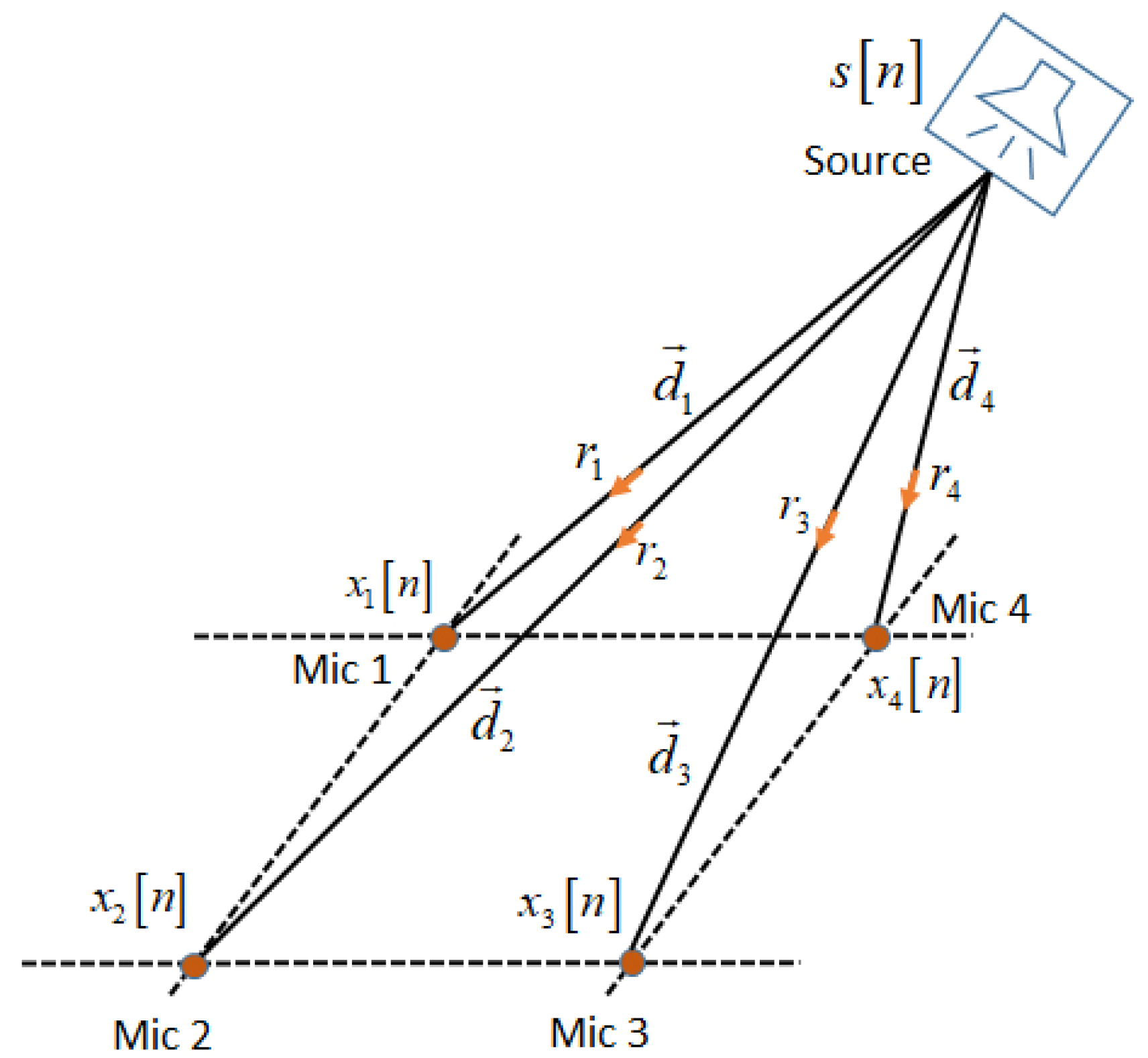
3.1. Microphone Signal Model in Localization Algorithms

The localization algorithms are evaluated under controlled conditions to determine the robustness and accuracy. Therefore, these algorithms are examined on real and simulated data. In the evaluations of localization algorithms, the microphone signals are modeled to be similar to real scenarios. Ideal and real models are considered for microphone signals in the evaluations for localization, tracking, and estimating the number of speakers. In the ideal model, the received signal to the microphone is a delayed and weakened version of source signal, namely:

$$x_m[n]=\frac{1}{r_m}s[n-{\tau }_m]+{\stackrel{⌣}{v}}_m[n],$$

(1)

where $x_m[n]$ is the received signal in the m-th microphone, $r_m$ is the distance between the sound source and m-th microphone,${\tau }_m$ is the delay to arrive signal from the source to m-th microphone, and ${\stackrel{⌣}{v}}_m[n]$ is the additive noise in the m-th microphone place. This model is considered ideal because the effects of indoor conditions and reverberations are not considered. Reverberation is an important and undesirable environmental factor that the localization algorithms are not valid without considering this effect. Therefore, the microphone signal model is designed to be similar to real conditions. The real model for microphone signals is expressed as [39]:

$$x_m[n]=s[n]\times {\mathsf{\Lambda }}_m[{\overrightarrow{d}}^{\left(s\right)},n]+{\stackrel{⌣}{v}}_m[n],$$

(2)

where ${\mathsf{\Lambda }}_m[{\overrightarrow{d}}^{\left(s\right)},n]$ is the impulse response between the source and m-th microphone, which contains the room reverberation effect and the speech signal attenuation because of the distance between the source and the microphone. The received signal in the m-th microphone is obtained by the convolution (*) between the source signal and room impulse response, which is highly similar to real scenarios. Also, the noise is considered as the same as the real conditions. Notice that the real model is selected for the simulations to make the results comparable to real environments.

The near-field and far-field assumptions are considered for the signal propagation in the environments. In the near-field assumption, the source is located near to the microphone array, where the signal arrives to microphones in a spherical shape. However, in the far-field assumption, the source signal is located far from the microphone array and the speech signal arrives to the array in a flat shape. The near-field assumption is selected for the simulations due to the consideration of the indoor condition, room dimension, and source location. Figure 1 shows the near-field model for speech signal propagation between source and microphone array.

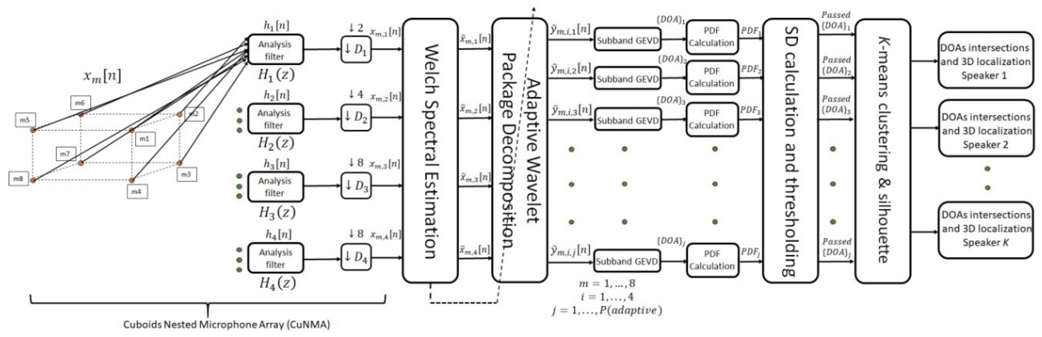
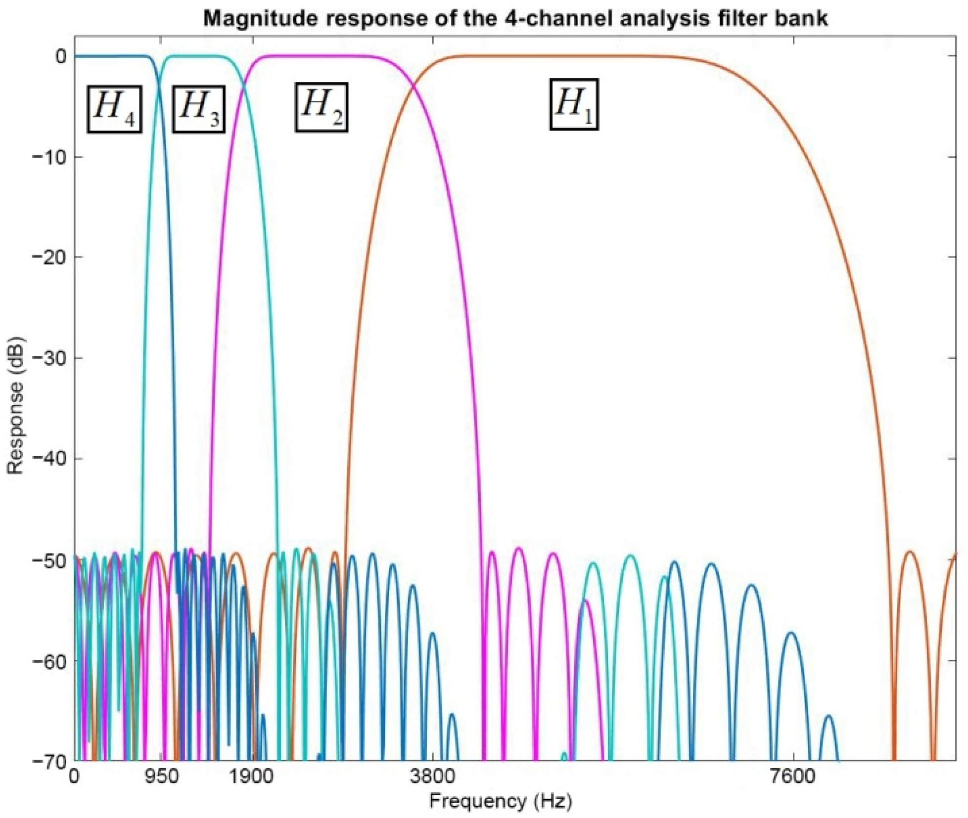
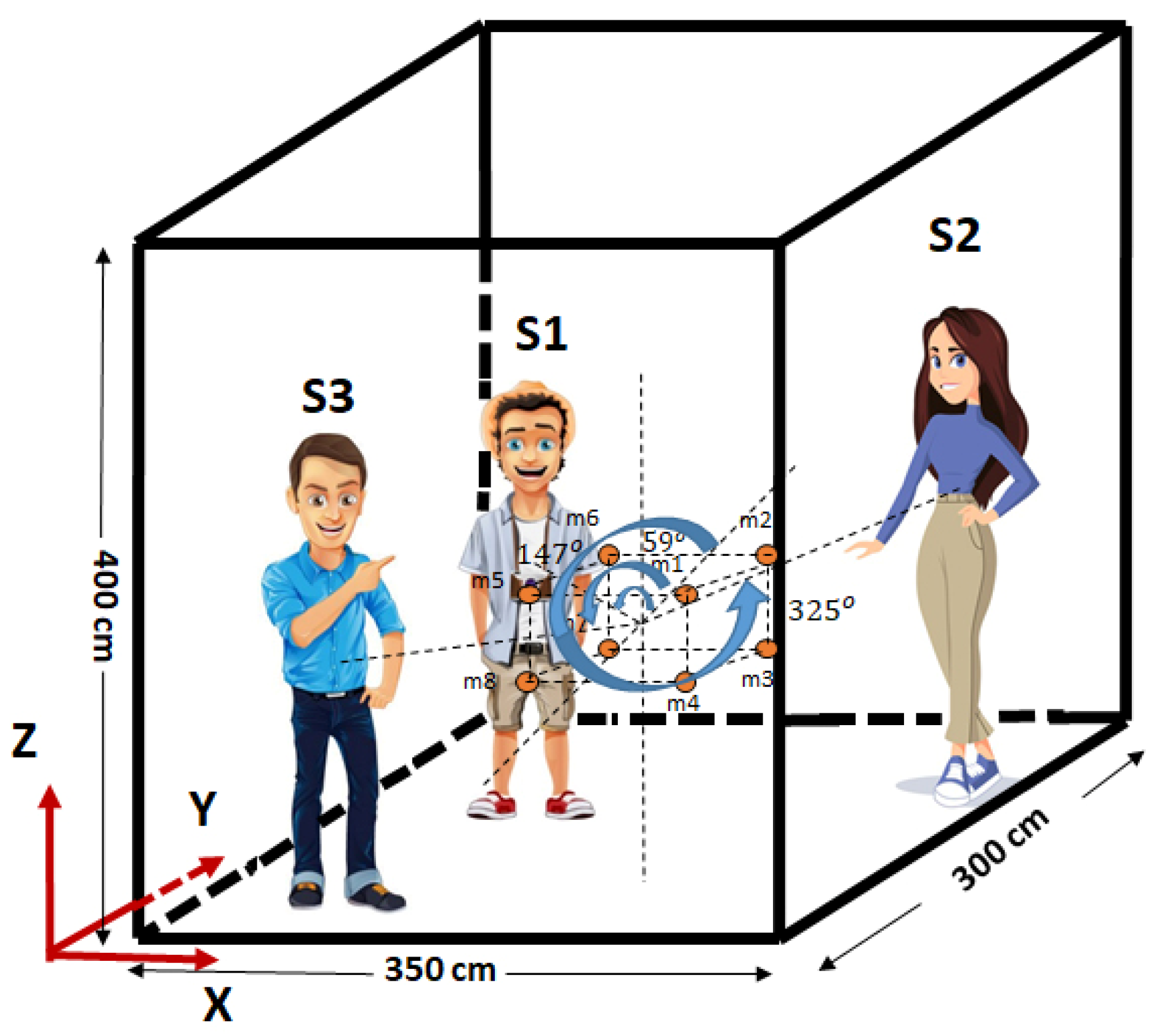
3.2. The Proposed Cuboids Nested Microphone Array for SSL

The spatial aliasing due to the inter-microphone distances in microphone arrays destroys the spectral information of speech signal and decreases the accuracy of the localization algorithms. The nested arrays are usually used in speech enhancement applications owing to their elimination of spatial aliasing. The linear microphone array was proposed for a speech enhancement algorithm in combination with adaptive noise canceller [40]. However, the linear nested array is not useful in localization applications because it does not prepare enough information for DOA estimations in different directions. In this section, a cuboids nested microphone array is proposed for the first time, which is applicable for 3D multiple simultaneous SSL. Each subarray is connected to the specific analysis filters. Figure 2 shows the block diagram of the proposed 3D localization method, where the CuNMA is shown in the left side of the diagram. The proposed CuNMA is designed to have the same characteristics for all speakers in different directions. There are enough microphone pairs in the direction of each speaker in this array [41]. Therefore, the proposed array does not make restrictions on the speaker’s locations.

The most spectral components of speech signal are in the frequency range [50–8000] Hz, with sampling frequency $F_s=\mathrm{16,000} \mathrm{Hz}$. The proposed CuNMA is designed to cover the frequency range [50–7600] Hz, which maintains the speech signal information. The proposed array is structured of 4 subarrays. The first subarray is designed for the highest frequency range B1 = [3800–7600] Hz. In this condition, the central frequency is $f{c}_1=5700 \mathrm{Hz}$ for analysis filter bank. The inter-microphone distance (d) follows the formula $d\le \lambda /2$ (where $\lambda$ is the wavelength associated with the maximum frequency of speech signal in the related subband) to avoid the spatial aliasing. Then, $d_1$ is calculated as follows $d_1\le \lambda /2=c/(2f)=342 (\mathrm{m}/\mathrm{s})/(2\times 7600 \mathrm{Hz})=2.3 \mathrm{cm}$ for the first subarray. The second subarray is structured for the frequency range B2 = [1900–3800] Hz The central frequency and inter-microphone distance are calculated as $f{c}_2=2850 \mathrm{Hz}$ and $d_2=2\times d_1\le 4.6 \mathrm{cm}$, respectively. The third subarray is designed to cover the frequency range B3 = [950–1900] Hz, where the inter-microphone distance is $d_3=4\times d_1\le 9.2\mathrm{cm}$ and the central frequency is $f{c}_3=1425 \mathrm{Hz}$. Finally, the fourth subarray is designed for the lowest frequency range B4 = [50–950] Hz. The central frequency and inter-microphone distance are $f{c}_4=500 \mathrm{Hz}$ and $d_4=8\times d_1\le 18.4 \mathrm{cm}$, respectively.

The CuNMA is designed to follow the above information. Then, the inter-microphone distance for the closest microphone pairs (1,2), (2,3), (3,4), (4,1), (5,6), (6,7), (7,8), and (8,5) is adjusted as $d_1=2.3 \mathrm{cm}$. The inter-microphone distance is $d_2=3.25 \mathrm{cm}$ for the second subarray with microphone pairs (1,3), (2,4), (5,7), and (6,8). This process is repeated for the third subarray with microphone pairs (4,7), (8,3), (5,4), (1,8), (6,1), (5,2), (6,3), and (2,7) with the inter-microphone distance $d_3=9.2 \mathrm{cm}$. Finally, the fourth subarray with microphone pairs (3,5), (6,4), (8,2), and (1,7) were designed with the inter-microphone distance $d_4=9.56 \mathrm{cm}$. Therefore, the spatial aliasing is eliminated by the proposed CuNMA without any effect on the speech signal information. Figure 3 shows the proposed CuNMA with microphone pairs related to each subarray. Four subarrays in this figure are designed based on the calculated microphone distances.

Each designed subarray in Figure 3 needs an analysis filter bank to prevent the spatial aliasing. The subarrays require a multirate sampling with a down sampler to design the appropriate filter for each subband. The analysis filter $H_i\left(z\right)$ and down sampler $D_i$ are implemented as a multilevel tree structure, which is shown in Figure 4. Each level of this tree includes a high-pass filter (HPF)$H{P}_i\left(z\right)$, a low-pass filter (LPF) $L{P}_i\left(z\right)$, and a down sampler $D_i$. The relationships between the analysis filter $H_i\left(z\right)$, high-pass filter $H{P}_i\left(z\right)$, and low-pass filter $L{P}_i\left(z\right)$ are expressed as [40]:

$$\begin{array}{l}{H}_1(z)=H{P}_1(z)\\ H_2(z)=L{P}_1(z)H{P}_2(z^2)\\ H_3(z)=L{P}_1(z)L{P}_2(z^2)H{P}_3(z^4)\\ H_4(z)=L{P}_1(z)L{P}_2(z^2)L{P}_3(z^4).\end{array}$$

(3)

In each level of the tree, a 52-tap LPF and a 52-tap HPF are selected, which are designed with Remez method based on the finite impulse response (FIR) filters. The filters have stop band attenuation −50dB and transition band 0.0647rad/s. Figure 5 shows the frequency response for analysis filter bank $H_i\left(z\right)$ related to designed microphone array. The filter $H_1\left(z\right)$ and $H_4\left(z\right)$ are implemented on the closest (subarray 1) and furthest (subarray 4) microphone pairs, respectively. Therefore, the microphone signals are prepared to enter the proposed system.

4. The Proposed Algorithm for Multiple SSL Based on SBGEVD

Multiple simultaneous SSL is a challenge in speech processing with unknown number of speakers in noisy and reverberant conditions. The proposed techniques for SSL should able to increase the accuracy of the algorithms with negligible computational complexity. In addition, the proposed method has to be resistant in noisy and reverberant conditions to prepare the trustable results for speaker localization. Since the speech is a W-DO signal, the main focus of the proposed method is subband processing based on the speech signal components. Subsequently, each block in the proposed algorithm in Figure 2 are explained in detail.

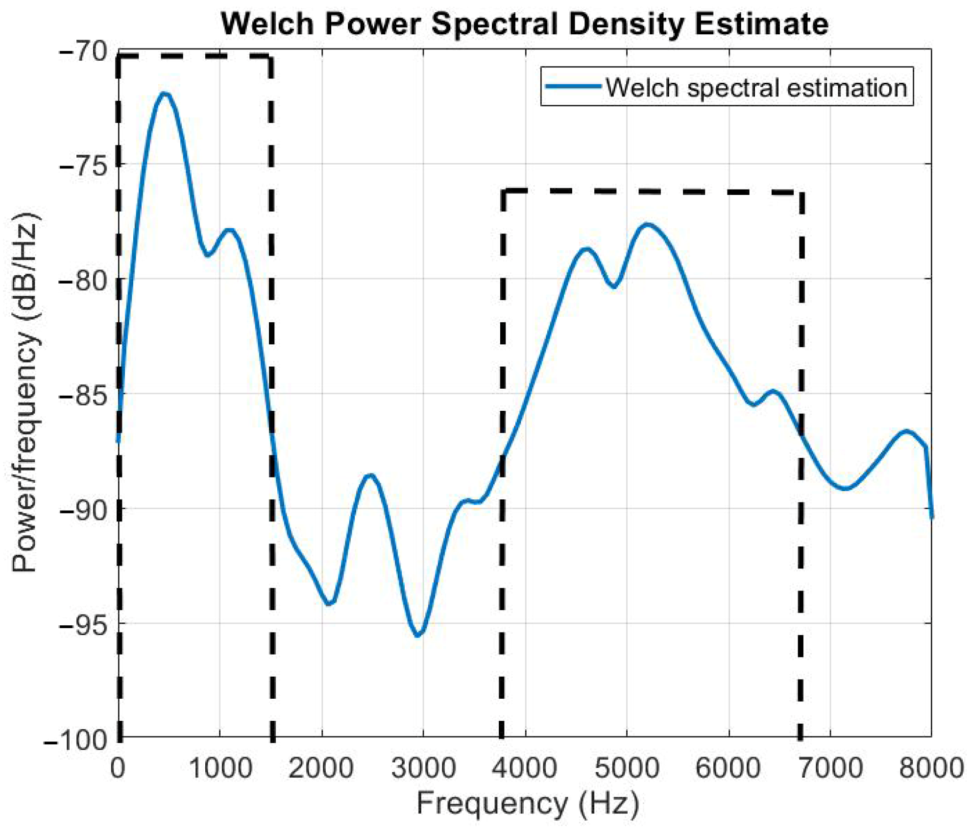
4.1. Spectral Estimation for Noise Reduction

Noisy speech spectral components decrease the accuracy of the speech processing algorithms such as localization and tracking. The speech spectral components are different in frequency bands. For example, the high frequency bands contain a few information of the speech signal while noise and reverberation have more effect in these components. The idea here is to propose a speech spectral estimation block for keeping the proper speech frequency components and for eliminating the undesirable components. Therefore, a spectral estimation block is considered in this section. The spectral estimation methods are divided into the parametric and non-parametric algorithms [42]. The non-parametric methods are based on the Fourier transform, which are calculated on a windowed signal before a smoothing method is implemented on these signals, such as periodogram and Welch. In parametric methods, the signal spectrum is modeled by a mathematic formula and the model’s parameters are estimated from the speech signal; finally, the signal spectrum is calculated via the following models: autoregressive (AR), moving average (MA), and autoregressive–moving-average (ARMA) methods. The experiments in [43] show that the Welch method prepares a smoother spectrum in comparison with other algorithms hence, it is considered in the proposed method in this article.

The Welch method was introduced to compensate the adverse effects of periodogram. In the Welch method, data blocking with overlapping and spectral averaging is considered for spectral estimation. String $\left\{x_{m,k}\right\}$ is assumed for $k=0,1,2,\dots ,N-1$. I blocks with length L are defined as:

$$x_{m,k}^i=x_m\left[k+(i-1)D\right],\mathrm{where}\{\begin{array}{l}m=1,\dots ,8\\ k=0,1,2,\dots ,L-1\\ i=0,1,2,\dots ,I\end{array},$$

(4)

where $x_{m,k}^i$ is the i-th block of string $\left\{x_{m,k}\right\}$, L is length of the block, and D is forward step (overlap rate). Each I block is multiplied by the window $w(k)$ and its periodogram is calculated.${\widehat{S}}^i(\omega )$ is the normalized periodogram for i-th block, which is defined as follows:

$${\widehat{S}}^i(m)=\frac{\mathsf{\Delta }t}{E_{w}L}{\left|{\displaystyle \sum _{k=0}^{L-1}{x}_{m,k}^{i}w(k)e^{-j\frac{2\pi km}{L}\mathsf{\Delta }t}}\right|}^{2}i=0,1,2,\dots ,I.$$

(5)

The normalization factor $E_w$ is the average window power, which is expressed as:

$$E_w=\frac{1}{L}{\displaystyle \sum _{k=0}^{L-1}{w}^2(k)}.$$

(6)

The Welch spectral estimation for power spectrum is defined as the average periodogram from I blocks, namely:

$$\widehat{S}(m)=\frac{1}{I}{\displaystyle \sum _{i=0}^{I-1}{\widehat{S}}^i(m)}.$$

(7)

The Welch method is similar to periodogram due to the bias but it is the enhanced version in terms of variance. If the signal length is enough, the non-overlapping data are considered for the Welch method, but the maximum 50% overlap is selected in the case of short data. Figure 6 shows an example of using Welch spectral estimation on a time frame of speech signal. As seen, the signal spectral amplitude is proper in some areas and is weak in others. The selected threshold for spectral amplitude in each frame is 30% of the maximum spectral amplitude in that frame. The areas with an amplitude lower than this value are denied from the localization process.

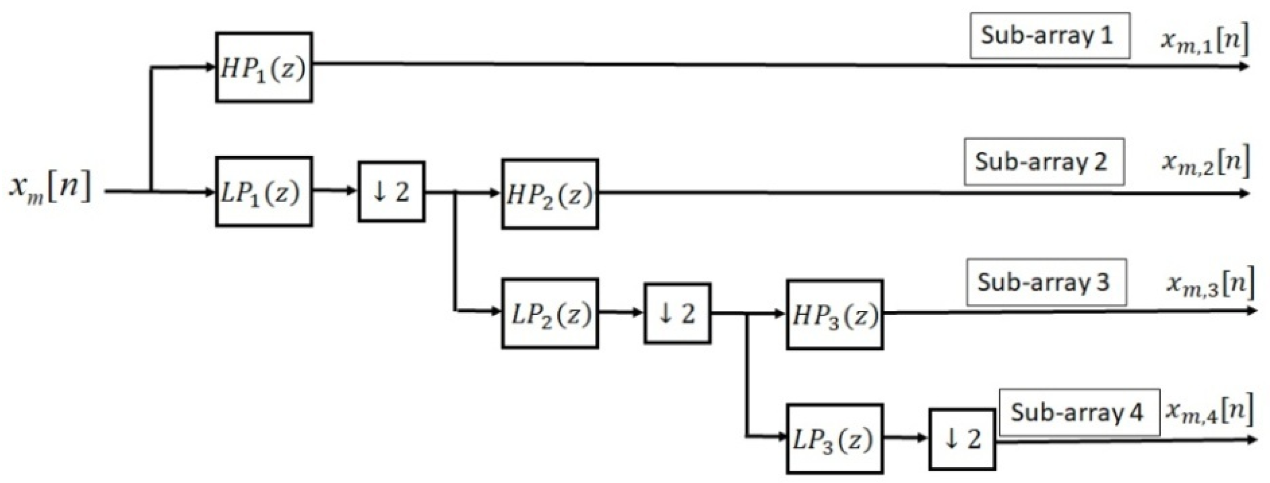
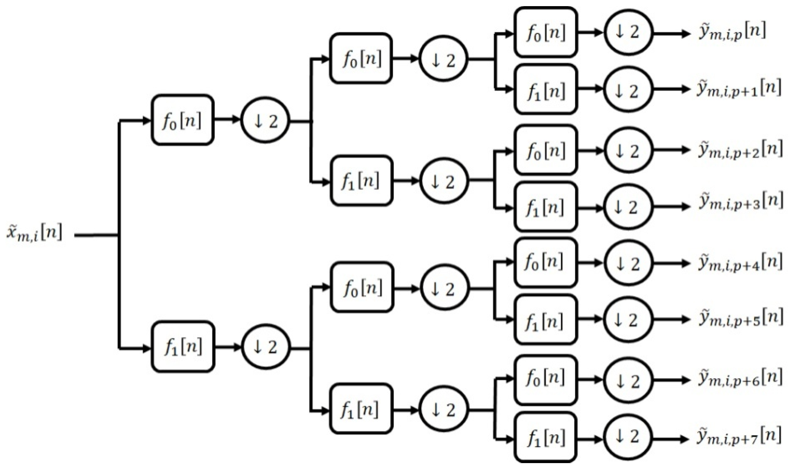
4.2. Adaptive Wavelet Transform

As mentioned, the speech spectral components depend on the frequency bands. Therefore, by paying better attention to each frequency band increases the accuracy of the localization algorithms. Since the speech signal is W-DO, with high probability there is just one speaker in narrow frequency bands. This property is considered for implementing the sub-band processing on speech signals. The sub-band divisions can be considered uniformly but speech is a non-stationary signal and, thus, its frequency information is variable during the time. Therefore, using the adaptive wavelet packet decomposition (AWPD) is proposed. The output of the Welch method is entered to the AWPD block. This adaptive wavelet is selected in the proposed system because of high and variable resolution in low frequency components related to the speech signal information. The Welch spectral estimation block output is shown as ${\tilde{x}}_{m,i}[n]$, where m is the microphone index $(m=1,\dots , 8)$ and i is the analysis filter index in CuNMA $(i=1,\dots ,4)$. Figure 7 shows the structure of the AWPD block for the applied method. This wavelet transform is adaptive because the number of levels and channels (p) are variable based on the estimated speech spectral components.

The continues wavelet transform (CWT) extracts the translation and scale coefficients from a continues signal. The obtained signal of CWT is highly capable to be used in TF analysis. CWT of continues signal $x\left(t\right)$ by the use of wavelet $\psi (t)$ is defined as [44]:

$$W\psi \left(s,\tau \right)={\displaystyle {\int }_{-\infty }^{+\infty }x\left(t\right){\overline{\psi }}_{s,\tau }^{}(t)dt},$$

(8)

where ${\psi }_{s,\tau }(t)$ is expressed as:

$${\psi }_{s,\tau }(t)=\frac{1}{\sqrt{s}}\psi (\frac{t-\tau }{s}),$$

(9)

where s and $\tau$ are scale and translation parameters, respectively and the over line denotes to the complex conjugate operator.$W\psi \left(s,\tau \right)$ is the wavelet coefficients and $\psi (t)$ denotes the mother wavelet, which is selected in different forms. The discrete wavelet transform (DWT) is considered as a powerful instrument in the speech signal processing. DWT can be expressed based on the CWT formulas. The only difference in DWT is the scale and translation parameters, which are written in power 2. The s and $\tau$ are considered as $s=2^a$ and $\tau =b\times 2^a$ where $\left(a,b\right)\in Z^2$; DWT is given by:

$${\psi }_{s,\tau }(t)=\frac{1}{\sqrt{2^a}}\psi \left(\frac{t-b\times 2^a}{2^a}\right).$$

(10)

The main part in DWT is the signal decomposition. The idea for decomposition in DWT is the use of LPFs and HPFs in combination with down samplers. The decomposition levels $a$ are selected based on the desired cut-off frequency. Figure 7 shows the structure of the wavelet package decomposition, where $f_0\left[n\right]$,$f_1\left[n\right]$ and $\downarrow 2$ are HPF, LPF, and down sampler with factor 2, respectively. The DWT input and output signals are considered as ${\tilde{x}}_{m,i}[n]$ and ${\tilde{y}}_{m,i,j}[n]$, respectively, where j is the number of created sub-bands by DWT on the input signal. The relation between LPF and HPF is written as:

$$f_1\left[n\right]={\left(-1\right)}^n{f}_0\left[G+1-n\right],$$

(11)

where G is the filter length with $n=0,1,\dots ,G$. There is not a certain method to select the mother wavelet. The mother wavelet selection is related to the input signal and application. Daubechies, Haar, Coiflet, Biorthogonal, Symlets, Morlet, and Mexican hat are the mother wavelets [45] where the Daubechies (Db4) is selected for the DWT in the proposed system because it has a proper performance on speech signals. Therefore, the AWPD is considered for subband processing and the speech signals are divided into high frequency resolution sub-bands for GEVD algorithm.

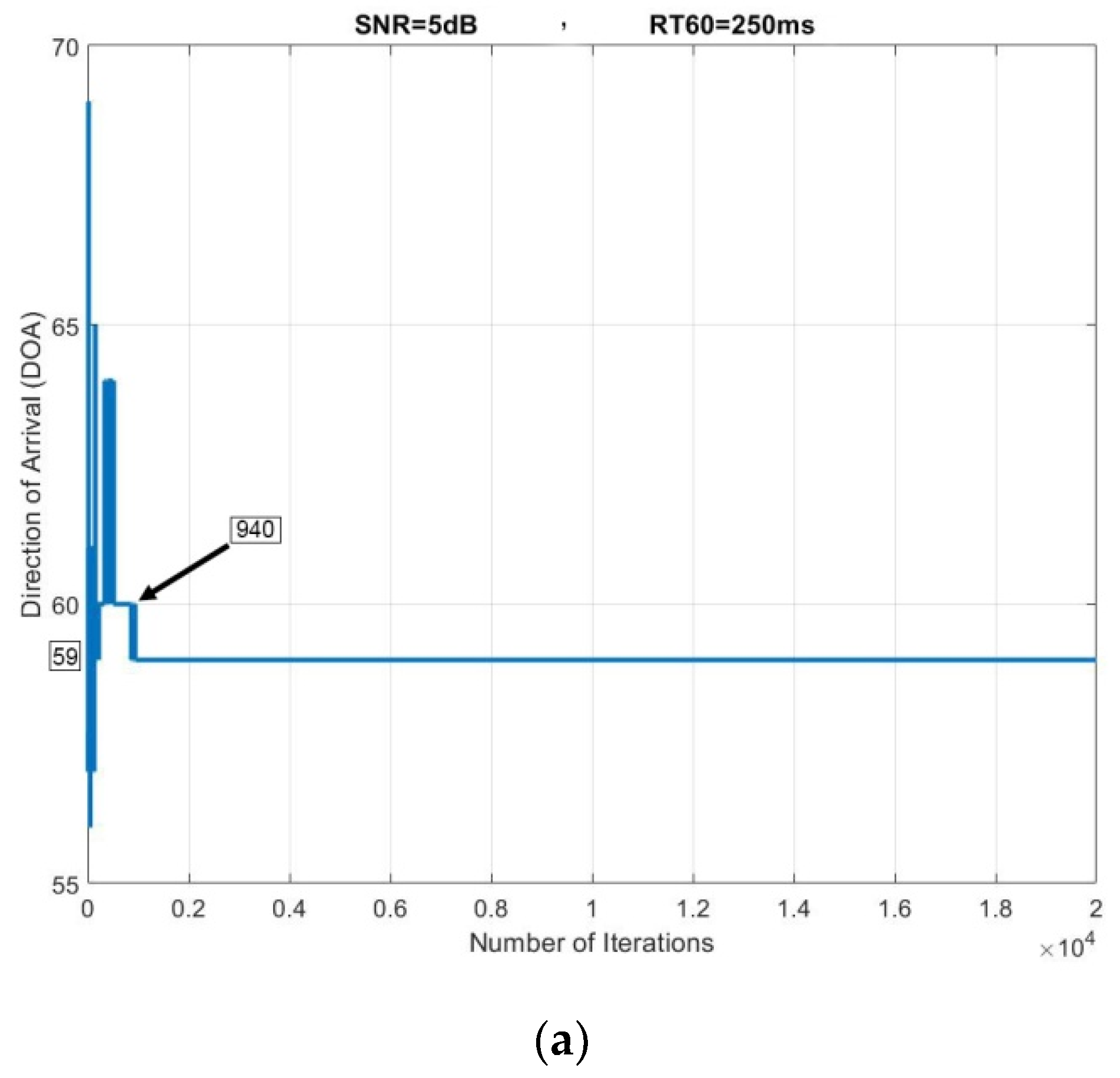
4.3. The Subband GEVD Algorithm for DOA Estimation

The SSL algorithm in this article is based on TDOA estimations from microphone pairs. The GEVD is a novel method for source localization, which is implemented in sub-bands on microphone pairs. The eigenvector related to the smallest eigenvalue of covariance matrix contains the impulse responses between the source and microphone signals, which are all required information for TDOA estimation [46]. If the room is considered as a linear and time invariant (LTI) system, signals for each microphone pair are written as:

$${\underset{\_}{x}}_1^T[n]\times {\underset{\_}{g}}_2={\underset{\_}{x}}_2^T[n]\times {\underset{\_}{g}}_1,$$

(12)

where ${\underset{\_}{x}}_1[n]$, ${\underset{\_}{x}}_2[n]$ are signal vectors, while ${\underset{\_}{g}}_1$ and ${\underset{\_}{g}}_2$ are the impulse responses for microphones 1 and 2, respectively. Then, signal ${\underset{\_}{x}}_i[n]$ is expressed as:

$${\underset{\_}{x}}_i[n]={[x_i[n],x_i[n-1],\dots ,x_i[n-M+1]]}^T,i=1,2.$$

(13)

As seen in Equation (13), the microphone signal ${\underset{\_}{x}}_i[n]$ is shown by M samples of this signal and T denotes the transposing of the vector. The impulse response vector with length M is introduced as:

$${\underset{\_}{g}}_i={[g_{i,0},g_{i,1},\dots ,g_{i,M-1}]}^T,i=1,2.$$

(14)

The linear property in Equation (12) comes from the fact that $x_i=g_i\times s(i=1,2)$. Therefore, it can be written as:

$$x_1\times g_2=s\times g_1\times g_2=x_2\times g_1.$$

(15)

The GEVD algorithm estimates the TDOA between each microphone pair by the use of the covariance matrix, which is expressed as follows:

$$R=\left(\begin{array}{cc}{R}_{x_1{x}_1}& R_{x_1{x}_2}\\ R_{x_2{x}_1}& R_{x_2{x}_2}\end{array}\right),$$

(16)

where the covariance matrix components are defined as:

$$R_{x_i{x}_j}=\mathrm{E}\{{\underset{\_}{x}}_i[n],{\underset{\_}{x}}_{{}_j}^T[n]\},i=1,2,$$

(17)

where E is the expected value. In the next, vector u with length 2M for estimating the impulse response is proposed as follows:

$$\underset{\_}{u}=\left(\begin{array}{l}{\underset{\_}{g}}_2\\ -{\underset{\_}{g}}_1\end{array}\right).$$

(18)

From Equations (12) and (16), it is clear that $R\underset{\_}{u}=0$, and vector u contains the eigenvector of covariance matrix R related to eigenvalue 0. The accurate estimation of vector u is not possible in real conditions because of the non-stationary of the speech signal and background noise. We assume that noise is stationary in short frames. Then, the noise covariance matrix in the silent part of the signal is considered for updating the formulas in the noisy speech frames. The GEVD method extracts the generalized eigenvector related to the smallest generalized eigenvalue of noise covariance matrix ($R_M^b$) and signal covariance matrix ($R_M^x$) by the use of stochastic gradient algorithms. The noise covariance matrix ($R_M^b$) is estimated from silence part of the signal. Therefore, it is not able to be updated in the frames by existence noise and speech simultaneously. The noise covariance matrix ($R_M^b$) is used for updating the formulas in noisy speech part of the signal.

The generalized eigenvector is calculated by minimizing the cost function ${\underset{\_}{u}}^T{R}_M^x\underset{\_}{u}$ in an iterative process instead of updating all matrix $R_M^b$ and $R_M^x$, and by use of generalized eigenvector related to the smallest generalized eigenvalue. Therefore, the error signal $e[n]$ is processed as:

$$e[n]=\frac{{\underset{\_}{u}}^T[n]{\underset{\_}{x}}_m[n]}{\sqrt{{\underset{\_}{u}}^T[n]R_M^b\underset{\_}{u}[n]}}=\frac{{\underset{\_}{u}}^T[n]{\underset{\_}{x}}_m[n]}{\left|\left|\sqrt{R_M^b}\underset{\_}{u}[n]\right|\right|},$$

(19)

where is obtained in an iterative process by least mean square error (LMS) algorithm as:

$$\underset{\_}{u}[n+1]=\underset{\_}{u}[n]-\mu e[n]\frac{\partial \underset{\_}{u}[n]}{\partial e[n]},$$

(20)

where $\mu$ is the adaptation step in this algorithm. The gradient of error signal $e[n]$ is calculated as follows:

$$\frac{\partial e[n]}{\partial \underset{\_}{u}[n]}=\frac{1}{\sqrt{{\underset{\_}{u}}^T[n]R_M^b\underset{\_}{u}[n]}}\left({\underset{\_}{x}}_m[n]-e[n]\frac{R_M^x\underset{\_}{u}[n]}{\sqrt{{\underset{\_}{u}}^T[n]R_M^b\underset{\_}{u}[n]}}\right).$$

(21)

Vector $\underset{\_}{u}[n]$ is calculated by replacing Equations (19) and (21) by Equation (20) as:

$$\underset{\_}{u}[n+1]=\underset{\_}{u}[n]-\frac{\mu }{{\underset{\_}{u}}^T[n]R_M^b\underset{\_}{u}[n]}\left({\underset{\_}{x}}_m[n]{\underset{\_}{x}}_{{}_m}^T[n]\underset{\_}{u}[n]-e^2[n]R_M^b\underset{\_}{u}[n]\right),$$

(22)

where the expected value of Equation (22) is calculated after convergence, then:

$$R_M^x\underset{\_}{u}[\infty ]=E\left\{e^2[n]\right\}{R}_M^b\underset{\_}{u}[\infty ],$$

(23)

where $\underset{\_}{u}[\infty ]$ is the generalized eigenvector related to the smallest generalized eigenvalue of matrixes $R_M^b$ and $R_M^x$. An extra normalization step is implemented at each iteration step to prevent error propagation, which is expressed as:

$$e[n]={\underset{\_}{u}}^T[n]{\underset{\_}{x}}_m[n],$$

(24)

and,

$$\widetilde{\underset{\_}{u}}[n+1]=\underset{\_}{u}[n]-\mu e[n]\{{\underset{\_}{x}}_m[n]-e[n]R_M^b\underset{\_}{u}[n]\}.$$

(25)

Finally, vector u is calculated as follows:

$$\underset{\_}{u}[n+1]=\frac{\widetilde{\underset{\_}{u}}[n+1]}{\sqrt{{\widetilde{\underset{\_}{u}}}^T[n+1]R_M^b\widetilde{\underset{\_}{u}}[n+1]}}.$$

(26)

Impulse responses ${\underset{\_}{g}}_1$ and ${\underset{\_}{g}}_2$ are calculated by estimating vector u. The signal in the source location is obtained by the deconvolution between these impulse responses and microphone signals. Also, the TDOA between each microphone pair is calculated by estimating vector u. The results section will show the convergence of the SBGEVD algorithm to the related TDOA for each sound sources. The GEVD algorithm is implemented on each sub-band (SBGEVD) and the TDOA (or DOA) values are calculated for all microphone pairs in sub-bands. The cumulative distribution function (CDF) is plotted for all calculated DOAs in each sub-band. The sub-bands with information for just one dominant speaker are selected by thresholding on these CDFs (or PFDs) and the other sub-bands with inappropriate information are denied. This thresholding is based on the SD calculation on data (DOAs) in each sub-band. The SBGEVD algorithm is iterated for each 3 continues frames and the SD is calculated for sub-band CDFs and this process is repeated for frequent time frames to cover one second of overlapped speech signal for multiple speakers. Therefore, the updated time is selected as one second for the proposed SSL algorithm. When the process is fully completed, all passed DOAs by the SD thresholding decision step are entered to the clustering for estimating the number of speakers and 3D SSL. The K-means clustering with silhouette criteria [47] are selected for the final step. The K-means algorithm is implemented on all passed DOAs of the SD decision step.

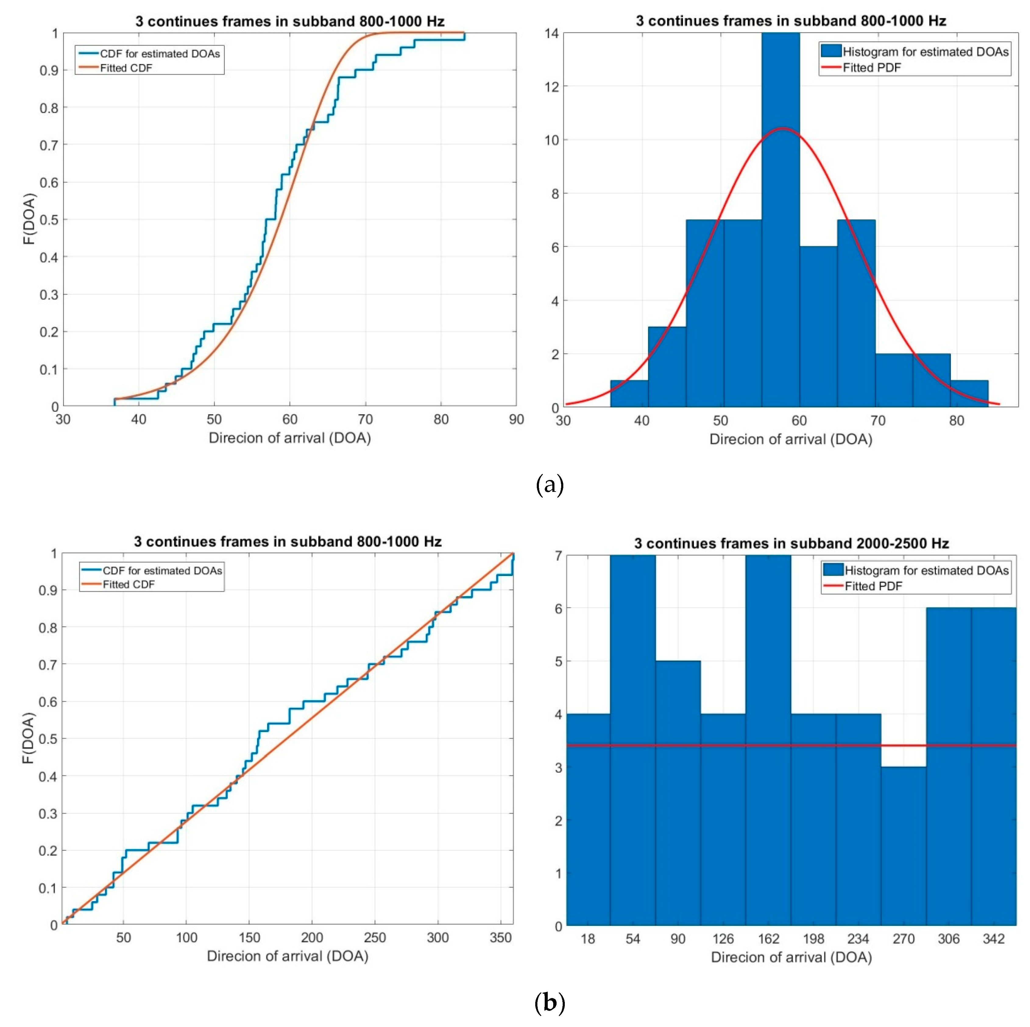
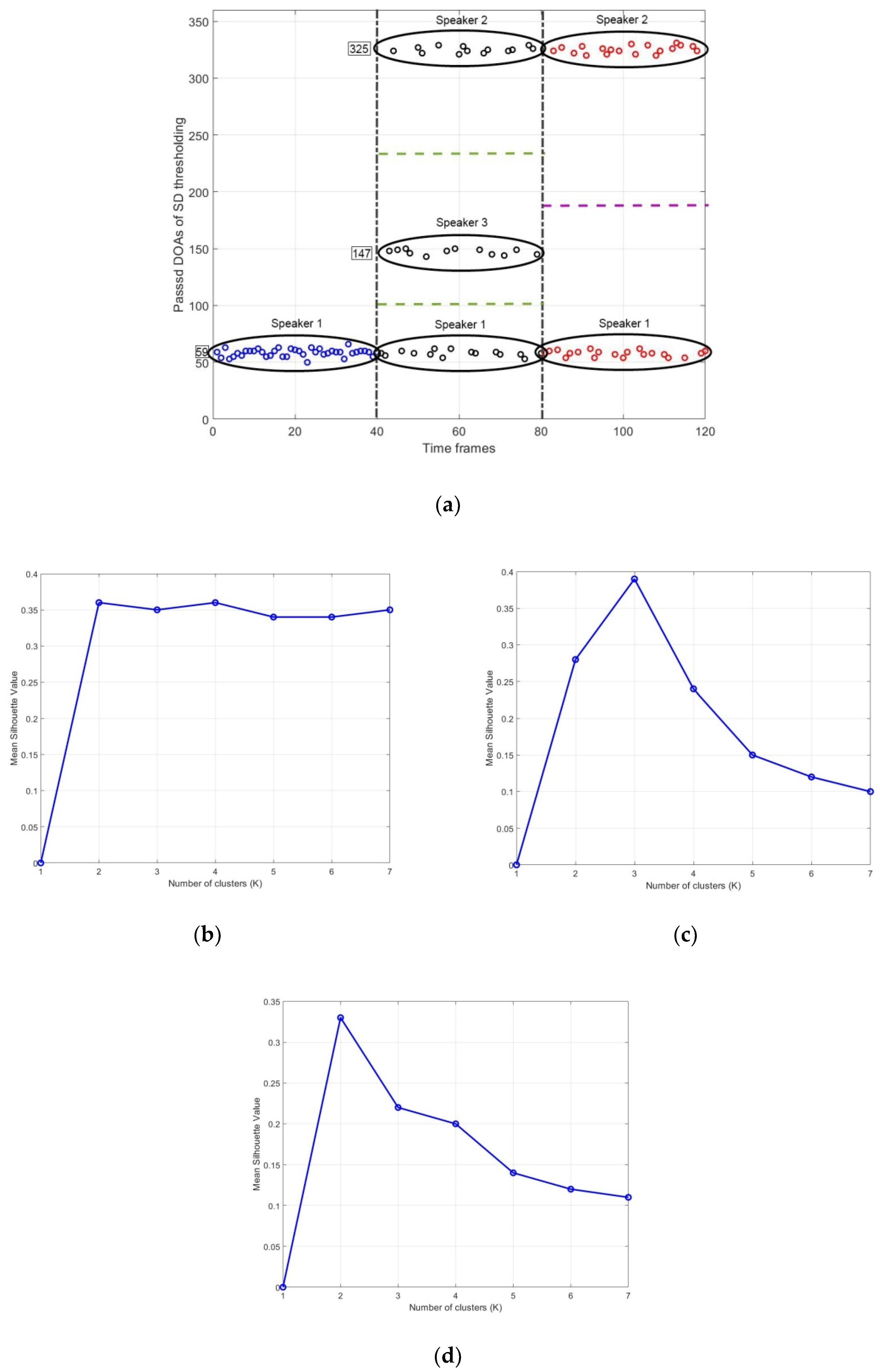
4.4. Clustering and 3D Sound Source Localization

K-means is an unsupervised clustering algorithm for data classification. The idea is to define K centroids, which are far from each other to have the best results. In the next step, each datum (the estimated DOAs by SBGEVD method and passed in the SD decision step) are associated with the closest centroids. Then, the centroids are recalculated by the associated data entire each cluster. The new centroids are calculated by averaging the existence data in each cluster. Therefore, the first data grouping is denied and the grouping step (associating data to the closest cluster) is iterated based on the new centroids. These steps are repeated until the centroids have no tangible changes. In other words, the aim is minimizing the following cost function:

$$J={\displaystyle \sum _{m=1}^{\mathrm{K}}{\displaystyle \sum _{n=1}^{N_k}{\Vert {\mathrm{DOA}}_n^{(m)}-C_m\Vert }^2}},$$

(27)

where ${\Vert {\mathrm{DOA}}_n^{(m)}-C_m\Vert }^2$ is the Euclidean distance between data ${\mathrm{DOA}}_n^{(m)}$ and centroid $C_m,$ and $N_k$ is the number of DOAs in each cluster. The main issue in K-means clustering is the estimation of the K-value. Therefore, the number of speakers is determined by estimating the K value and, finally, the 3D position of each speaker is estimated by the intersection between DOAs in each cluster. The silhouette criteria are considered for estimating the K value in the proposed method.

Silhouette criteria is a method for validating the associated data to the clusters. This method shows graphically if the data is adjusted to the proper cluster or should be associated to another cluster. We assume that data have been clustered with a specific K value. For each data i,$v(i)$ is defined as the average dissimilarity between data i and all data in the same cluster. The Euclidean distance is selected for this measurement. The smaller $v(i)$ value shows the better adjustment of data i in its cluster. The average dissimilarity $v(i)$ of data i to the centroid $C_m$ is defined as the average distance between data i and all other data in the same cluster. We define $c(i)$ as the lowest average dissimilarity of data i with other clusters that data i is not a member of them. The cluster with smallest $c(i)$ value is selected as a neighbor cluster for data i because is the best cluster for data i if it does not adjust well in the current cluster. The silhouette value,$Z(i)$, for data i is defined as:

$$Z(i)=\frac{c(i)-v(i)}{\max \left\{v(i),c(i)\right\}}.$$

(28)

$Z(i)$ can be simplified mathematically as:

$$Z(i)=\{\begin{array}{l}1-\frac{v(i)}{c(i)}ifv(i)<c(i)\\ 0ifv(i)=c(i)\\ \frac{c(i)}{v(i)}-1ifv(i)>c(i).\end{array}$$

(29)

If $v(i)\ll c(i)$,$Z(i)$ value becomes close to 1. Since $v(i)$ is the average dissimilarity of data i to its cluster, this value shows that data i is adjusted properly to the cluster. Moreover, a large value of $c(i)$ explains that data i has not been adjusted well with its cluster. If $Z(i)$ is close to −1, then it is better than data i transfers to the neighbor cluster. The means that the silhouette value $Z(i)$ is a criterion for validating an unsupervised clustering algorithm on a series of data. In the results and discussions section, the means silhouette value (MSV) is shown for various K values and signal frames. The pick position in the MSV plot refers to the number of speakers that K is the index of pick value. If the MSV curve has no maximum, the number of speakers is considered as 1. Each cluster represents one speaker. In the next, the DOAs in each cluster are plotted as a plane and the intersections are calculated. This process is repeated for all clusters to obtain the 3D position for all K speakers as:

$$({\widehat{x}}_k,{\widehat{y}}_k,{\widehat{z}}_k)={\left\{{\mathrm{DOA}}_{k,1}\cap {\mathrm{DOA}}_{k,2}\cap \dots \cap {\mathrm{DOA}}_{k,n}\right\}}_{k=1,\dots ,\mathrm{K}}^{n=1,\dots ,N_k},$$

(30)

where K is the number of speakers and $N_k$ is the number of DOAs in cluster k that the 3D location of speaker k is represented as $({\widehat{x}}_k,{\widehat{y}}_k,{\widehat{z}}_k)$. Therefore, the accuracy of localization algorithm is increased by the cuboids nested microphone array, sub-band processing on GEVD method, SD thresholding by making a decision on DOA values, and intersections between DOAs in each cluster for estimating the 3D positions.

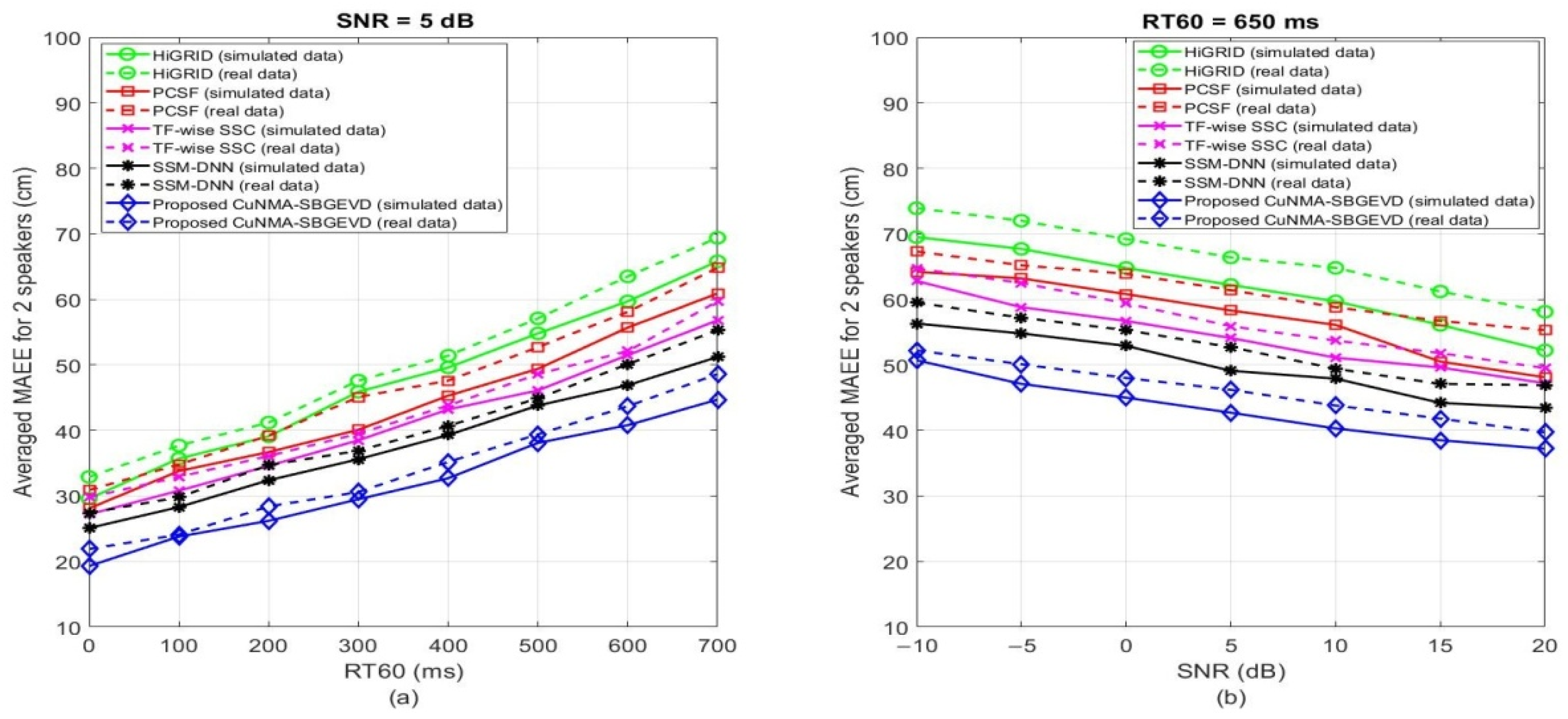
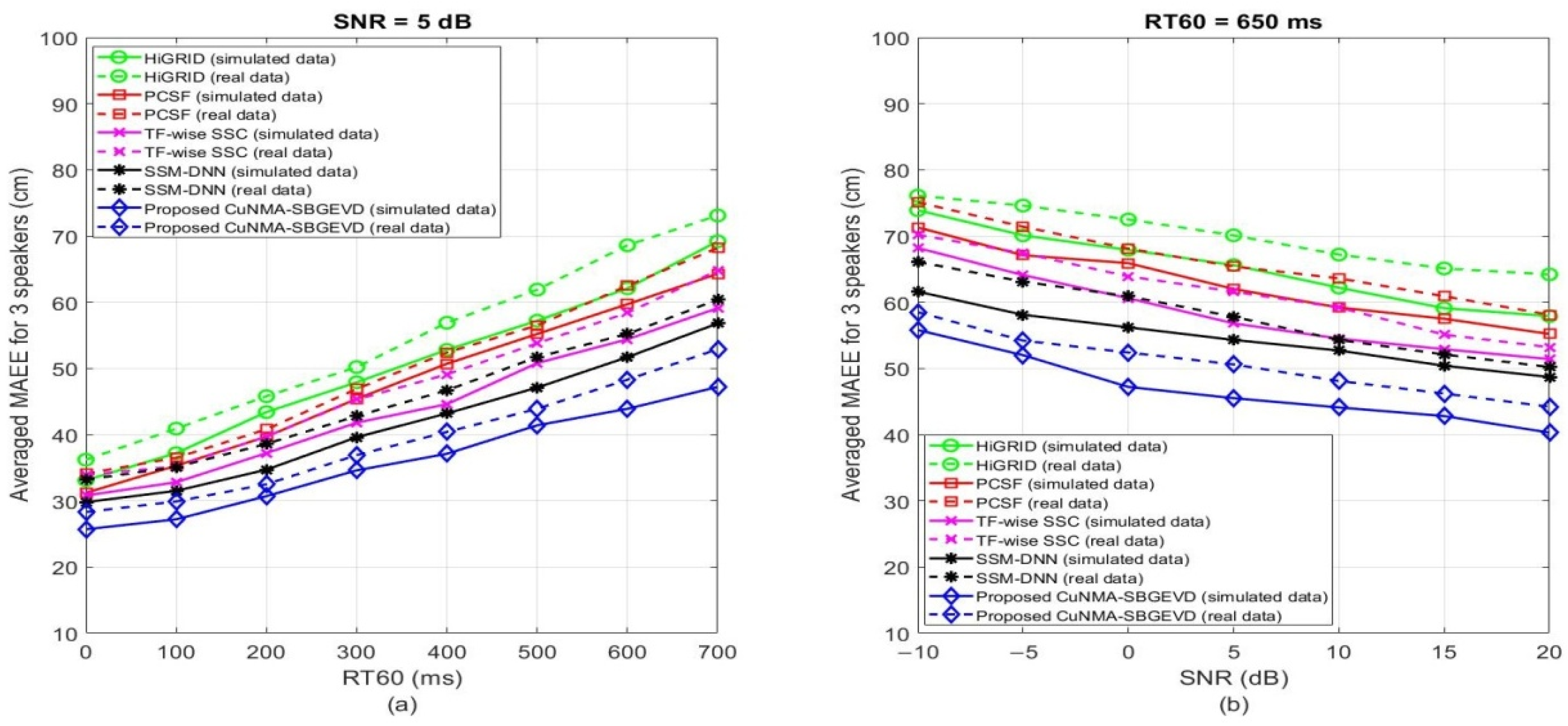
5. Results and Discussions

The experiments are implemented on real and simulated data for evaluating the proposed multiple simultaneous SSL algorithm. The Texas Instruments and Massachusetts Institute of Technology (TIMIT) dataset is considered for simulated data in evaluations [48]. The proposed algorithm is implemented on the overlapped speech signal. In the real condition, for about 90% of overlapped speech is from two simultaneous speakers. Almost 8% of overlapped speech is from 3 simultaneous speakers and the rest is for four and more simultaneous speakers [49]. As seen, around 98% of overlapped speech signal is just for two and three simultaneous speakers. Therefore, the simulations are implemented for the scenarios with two and three speakers. Then, one male and one female speaker (S1 and S2) are considered for two simultaneous speakers and two males, and one female speaker are selected for three overlapped speakers. Also, the evaluations are implemented on real data, which are recorded at a speech processing laboratory, at the Universidad Tecnológica Metropolitana, to compare the results between the simulated and real conditions. The microphone signals are recorded in the acoustic room by a cuboids nested 8-microphones array, located in the middle of room. The microphones are connected to a recording speech system, which captures the synchronized signals simultaneously. Also, the connected speakers to separate computers are considered instead of humans in the recording room for better control of the transmitted signal power. The speech signals are played by the speakers in front of CuNMA and they are recorded by the microphones. In the simulations, 45 s speech signal is considered for each speaker that 27.2 s of the signals have overlap between 2 speakers and 20.6 s of the overlapped signals are for three simultaneous speakers. Figure 8 shows the speech signal for each speaker jointly with two and three overlapped signals.

The simulation conditions are adjusted to be similar to real scenarios. Therefore, the room dimension is set as (350, 300, 400) cm. The three speakers are located at (60,220,170) cm (S1), (310,245,175) cm (S2) and (95,75,180) cm (S3), respectively. In addition, the CuNMA is placed in the middle of room that the center of the array is located at (175,150,120) cm. Figure 9 shows a view of the room with locations of the speakers and microphone array. The microphone positions, speakers’ locations, and room dimensions are summarized in

Table 1. Microphones positions, speakers’ locations and room dimension.

Positions	X, cm	Y, cm	Z, cm
Microphone 1 (m1)	179.5	148.8	121.2
Microphone 2 (m2)	179.5	151.1	121.2
Microphone 3 (m3)	179.5	151.1	118.9
Microphone 4 (m4)	179.5	148.8	118.9
Microphone 5 (m5)	170.5	148.8	121.2
Microphone 6 (m6)	170.5	151.1	121.2
Microphone 7 (m7)	170.5	151.1	118.9
Microphone 8 (m8)	170.5	148.8	118.9
Speaker 1	60	220	170
Speaker 2	310	245	175
Speaker 3	95	75	180
Room Dimension	350	300	400

.

Noise and reverberation are two important factors that decrease the accuracy of localization algorithms. These two factors are observed clearly in the real conditions. Therefore, we should consider these factors in the simulated scenarios. White Gaussian noise with variable power is selected for simulations to create the noisy signal with different signal-to-noise ratio (SNR). This Gaussian noise models the real noisy environment in the simulated data. The Image model is selected for the simulations to prepare the reverberation effect as same as the real conditions [50]. The Image model creates the reverberations in the indoor conditions similar to the real environments with high accuracy. This model estimates the room impulse response between source and microphone by considering room dimensions, microphone location, source position, impulse response length, sampling frequency, surface reflection coefficients, and reverberation time ($R{T}_{60}$). The received signal in the microphone place is generated by the convolution between the generated room impulse response and source signal. The room reverberation time is easily changeable in simulations, but it is hard to change $R{T}_{60}$ in real conditions. The absorbent panels are used on the walls and floors to change the room reverberation time in real scenarios. The $R{T}_{60}$ value changes by moving the location, increasing and decreasing the number of panels.

The experiments are implemented on environmental scenarios. Then, three main scenarios are designed for the evaluations. The first scenario is reverberant environment with $R{T}_{60}=650 \mathrm{ms}$ and $SNR=20 \mathrm{dB}.$ The noisy scenario has dominant noise against reverberation as $SNR=5 \mathrm{dB}$ and $R{T}_{60}=250 \mathrm{ms}.$ Finally, the most challenging scenario is noisy-reverberant with $SNR=5 \mathrm{dB}$ and $R{T}_{60}=650 \mathrm{ms}.$ Also, the experiments are done on fixed-SNR values and variable $R{T}_{60}$ and vice versa for evaluating the robustness of the proposed method during the SNR and $R{T}_{60}$ changes. The simulations are done on MATLAB software version 2019b (MathWorks, Natick, MA, USA). Also, the experiments are implemented on PC with CPU core i7-7700 (Intel, Santa Clara, CA, USA), 4.2 GHz and 32 GB RAM. The Hamming window with 60ms length and 50% overlap is considered to prepare the constant frames of speech signal that the speaker positions are fixed during this short time. Therefore, the sufficient and trustable information is prepared for the proposed algorithm. The proposed CuNMA-SBGEVD method is compared with HiGRID [33], PCSF [35], TF-wise SSC [37] and SSM-DNN [36] methods to show the precision and robustness of the estimated locations in comparison with previous works. Also, the mean absolute estimation error (MAEE) criteria between the true $(x_k,y_k,z_k)$ and estimated $({\widehat{x}}_k,{\widehat{y}}_k,{\widehat{z}}_k)$3D locations, in cm, is calculated for $N_f$ continuous frames and for speaker k to compare results in noisy and reverberant scenarios.

$${\mathrm{MAEE}}_k=\frac{1}{N_f}{\displaystyle \sum _{q=1}^{N_f}\left|(x_{k,q},y_{k,q},z_{k,q})-({\widehat{x}}_{k,q},{\widehat{y}}_{k,q},{\widehat{z}}_{k,q})\right|}$$

(31)

One of the main parts of the proposed system is the SBGEVD block. The final localization results are related directly to the convergence of DOA values in this part. Figure 10 shows the convergence curve for the SBGEVD algorithm in sub-band 1.8–2 kHz and for noisy, reverberant, and noisy-reverberant scenarios for the first speaker. As seen in this Figure, the SBGEVD function is converged to the correct DOA ${59}^{\mathrm{o}}$ for the first speaker in all three scenarios. These correct convergences are due to the sub-band processing with spectral estimation in the pre-processing step. The speed of convergence in noisy scenario is more than the reverberant scenario and noisy-reverberant scenario, which has the lowest speed of convergence because of the existence of both undesirable factors at the same time. Also, in the sub-bands with simultaneous speakers, the DOA is not converged to the correct value and it makes errors in the estimated location. Therefore, the sub-bands with simultaneous speakers are denied in the next step.

The CDF and PDF calculations are another block in the proposed CuNMA-SBGEVD algorithm, which are implemented on the estimated DOAs from each sub-band. The CDFs (and finally PDFs) are calculated to show a robust distribution of DOAs in sub-bands. Figure 11 shows the CDFs and PDFs for sub-bands 0.8–1 kHz and 2–2.5 kHz and for three continuous time frames. As shown in Figure 11a, the PDF is closer to Gaussian distribution and it means the estimated DOAs in this subband are centralized around a specific point (the DOA for first speaker ${59}^{\mathrm{o}}$). The calculated SD in this condition is a small value. Figure 11b shows the CDF and PDF for a sub-band, which contains the mixing of speaker information and the estimated DOA does not present a correct direction. Therefore, the PDF curve is closer to uniform distribution and SD is a larger value in this condition. This means that the estimated DOAs in this sub-band are not trustable and will be denied. Based on the experiments, the threshold value for the SD to accept or reject the DOAs in sub-bands is $\pm {10}^{\mathrm{o}}$. Therefore, the estimated DOAs for the sub-band with the SD of PDF function under $\pm {10}^{\mathrm{o}}$ are passed to the clustering step and the rest are denied. Then, the proper estimated DOAs are considered for the clustering process to decrease the localization error. Finally, the intersection between passed DOAs in each cluster represent the 3D position of each speaker.

Finally, the last step of the proposed method is K-means clustering jointly with silhouette criteria for estimating the number of speakers and 3D SSL. Therefore, simulations are implemented on three areas of speech signal for single, two, and three simultaneous speakers to show the superiority of the proposed method. Figure 12 shows the results for clustering and silhouette criteria in $SNR=20 \mathrm{dB}$ and $R{T}_{60}=250 \mathrm{ms}$(low level of noise and reverberation). Figure 12a represents the approved DOAs from thresholding on sub-band PDFs. The K-means algorithm is implemented on all of these data. Also, the silhouette criteria are considered to select the best K for all regions of data. Figure 12b–d shows the results for silhouette criteria in the time domain. Figure 12b represents the MSV curve for the first region (left side) of Figure 12a, which shows the existence of just one speaker because of not having any outstanding maximum in different K values. The 3D source location is estimated by this clustering and the intersection between DOAs as (51,229,168) cm with 12.88 cm error in comparison with correct location (60,220,170) cm. This process is iterated for the second region (center) in Figure 12a that the MSV curve is shown in Figure 12c. As shown in this Figure, the MSV curve is maximized in K = 3 by showing the existence of three speakers in this area. The locations for three speakers are estimated by the intersection between DOAs in the three clusters as (66,215,176) cm (S1), (321,230,184) cm (S2) and (102,71,172) cm (S3) which have 9.84 cm, 20.66 cm, and 11.35 cm errors with correct locations (60,220,170) cm (S1), (310,245,175) cm (S2) and (95,75,180) cm(S3), respectively. Finally, the silhouette criteria is implemented for the last region of Figure 12a, which is shown in Figure 12d with maximum in K = 2 and existence of two speakers (speakers 1 and 2) in this region. The speakers’ locations are estimated by the intersection between DOAs in each cluster, which shows the location (58,227,161) cm and (302,253,181) cm for the first and second speakers, respectively. The correct locations for these two speakers are (60,220,170) cm (S1) and (310,245,175) cm (S2), respectively, which have11.57 cm and 12.8 cm errors with the estimated locations.

Table 2. The mean absolute estimation error (MAEE) comparison between the proposed cuboids nested microphone array (CuNMA)-subband generalized eigenvalue decomposition(SBGEVD) and hierarchical grid (HiGRID), perpendicular cross-spectra fusion (PCSF), time-frequency wise spatial spectrum clustering (TF-wise SSC), and spectral source model-deep neural network (SSM-DNN) methods for reverberant, noisy, and noisy-reverberant scenarios on real and simulated data for 2 simultaneous speakers.

MAEE (cm)	HiGRID [33]		PCSF [35]		TF-Wise SSC [37]		SSM-DNN [36]		Proposed CuNMA-SBGEVD
Simulated Data
Speaker	S1	S2	S1	S2	S1	S2	S1	S2	S1	S2
Scenario 1	51	53	46	50	45	49	43	44	36	38
Scenario 2	40	44	37	39	34	38	32	36	25	29
Scenario 3	59	65	55	61	54	55	48	51	41	43
Real Data
Speaker	S1	S2	S1	S2	S1	S2	S1	S2	S1	S2
Scenario 1	55	62	55	54	46	52	45	47	37	41
Scenario 2	43	46	41	44	36	39	36	33	26	30
Scenario 3	64	68	61	63	53	61	44	54	45	46

shows the results for the proposed CuNMA-SBGEVD algorithm in comparison with HiGRID, PCSF, TF-wise SSC, and SSM-DNN methods in reverberant, noisy, and noisy-reverberant scenarios on real and simulated data for two simultaneous speakers. The MAEE criteria, in cm, is considered for measuring the error in the estimating of 3D speaker locations on 20 continuous frames. Based on the MAEE values in this table, the noisy environment has better results in comparison with two other scenarios. Also, the simulated data have less MAEE in comparison with real data because of the better control of environmental parameters (noise and reverberation). In addition, the proposed CuNMA-SBGEVD has a better accuracy in most of the scenarios in comparison with previous works. In scenario 3, for real data, the SSM-DNN method has a slight smaller MAEE, which cannot be extended to all scenarios.

Figure 13 shows the averaged MAEE results for the proposed CuNMA-SBGEVD in comparison with HiGRID, PCSF, TF-wise SSC, and SSM-DNN methods for different range of SNRs and $R{T}_{60}$ on real and simulated data for 2 simultaneous speakers. Figure 13a represents the averaged MAEE for $SNR=5 \mathrm{dB}$ and $0<R{T}_{60}<700 \mathrm{ms}$. As seen, the proposed method has less MAEE in comparison with other previous works on real and simulated data. For example, in $R{T}_{60}=700 \mathrm{ms}$, the averaged MAEE for the proposed CuNMA-SBGEVD method on the simulated data is 44 cm in comparison with 65 cm for HiGRID, 60 cm for PCSF, 56 cm for TF-wise SSC, and 51 cm for SSM-DNN, which shows the higher accuracy of the proposed method in contrast to other methods. Also, Figure 13b shows these results for $R{T}_{60}=650 \mathrm{ms}$ and $-10<SNR<20 \mathrm{dB}$. As shown, the proposed method has a better accuracy in all of the conditions in comparison with other works. For example, in $SNR=5 \mathrm{dB}$, the averaged MAEE is 42 cm for the proposed CuNMA-SBGEVD in comparison with 62 cm for HiGRID, 58 cm for PCSF, 54 cm for TF-wise SSC, and 49 cm for SSM-DNN algorithms for simulated data, thus showing the superiority of the proposed method.

Table 3. The MAEE comparison between the proposed CuNMA-SBGEVD method and HiGRID, PCSF, TF-wise SSC, and SSM-DNN algorithms in reverberant, noisy, and noisy-reverberant scenarios on real and simulated data for 3 simultaneous speakers.

MAEE (cm)	HiGRID [33]			PCSF [35]			TF-wise SSC [37]			SSM-DNN [36]			Proposed CuNMA-SBGEVD
Simulated Data
Speaker	S1	S2	S3	S1	S2	S3	S1	S2	S3	S1	S2	S3	S1	S2	S3
Scenario 1	55	54	59	53	56	58	48	50	54	43	48	47	41	39	44
Scenario 2	43	46	47	39	43	44	39	42	40	34	37	39	28	29	32
Scenario 3	65	67	64	58	63	61	57	56	59	54	56	54	39	42	49
Real Data
Speaker	S1	S2	S3	S1	S2	S3	S1	S2	S3	S1	S2	S3	S1	S2	S3
Scenario 1	65	63	69	59	55	61	53	51	56	45	53	50	38	45	43
Scenario 2	45	47	51	43	44	46	38	42	44	35	42	43	29	34	35
Scenario 3	68	71	72	59	65	68	59	65	61	53	57	59	42	51	50

represents the MAEE results for the proposed CuNMA-SBGEVD method in comparison with HiGRID, PCSF, TF-wise SSC, and SSM-DNN for 3 simultaneous speakers in reverberant, noisy, and noisy-reverberant scenarios on real and simulated data. The results are obtained from 20 continuous frames of overlapped speech signals. The results show the accuracy of the proposed method in the 3D localization in comparison with previous works. Also, the results in noisy scenarios are better than reverberant and noisy-reverberant conditions in all methods. In addition, the accuracy of the localization is higher for the closer speakers to the CuNMA because of the signal high power and low reverberation. The results for the simulated data are better than the real data because there is more accurate control of undesirable conditions in the simulations.

Figure 14 represents the averaged MAEE results for the proposed CuNMA-SBGEVD method and HiGRID, PCSF, TF-wise SSC, and SSM-DNN algorithms for 3 simultaneous speakers and various range of SNRs and $R{T}_{60}$. Figure 14a shows the averaged MAEE for $SNR=5 \mathrm{dB}$ and $0<R{T}_{60}<700 \mathrm{ms}$. As seen, the proposed method has high accuracy on real and simulated data in comparison with other previous works. For example, in $R{T}_{60}=700 \mathrm{ms}$,the averaged MAEE for the proposed CuNMA-SBGEVD method on the simulated data is 47 cm, which is more accurate in comparison with averaged MAEE 69 cm for HiGRID, 64 cm for PCSF, 59 cm for TF-wise SSC, and 56 cm for SSM-DNN. In addition, Figure 14b represents the results for $R{T}_{60}=650 \mathrm{ms}$ and $-10<SNR<20 \mathrm{dB}$. This experiment evaluates the noise effect on the proposed SSL method. As shown, the proposed method has the lowest averaged MAEE and higher precision in SSL in comparison with previous works. For example, in $SNR=5 \mathrm{dB}$, the averaged MAEE for the proposed CuNMA-SBGEVD on simulated data is 45 cm in comparison with 65 cm in HiGRID, 62 cm in PCSF, 55 cm in TF-wise SSC, and 53 cm in SSM-DNN algorithms.

Table 4. Comparison of computational complexity between the proposed CuNMA-SBGEVD, HiGRID, PCSF, TF-wise SSC, and SSM-DNN algorithms on real data for 2 and 3 simultaneous speakers (run-time in second).

Run-time (s)	HiGRID [33]	PCSF [35]	TF-wise SSC [37]	SSM-DNN [36]	Proposed CuNMA-SBGEVD
2 Simultaneous Speakers
Scenario 1	641	548	446	589	453
Scenario 2	592	529	419	557	438
Scenario 3	668	570	474	612	462
3 Simultaneous Speakers
Scenario 1	693	596	466	607	459
Scenario 2	659	572	437	582	448
Scenario 3	724	634	495	637	483

compares the computational complexity of the proposed CuNMA-SBGEVD in comparison with other previous works based on the run-time of MATLAB software in second. The experiments are implemented on real data for two and three simultaneous speakers. As seen, the HiGRID method has the highest computational complexity values because of searching the candidate places by the indoor conditions. After this method, PCSF and SSM-DNN algorithms have lower complexities in comparison with HiGRID but the SSM-DNN method still has the higher complexity because of using training and testing steps in the DNN structure. The complexity of the proposed method is similar to the TF-wise SSC algorithm, but in some conditions, the proposed method has less complexity. This can be justified by the use of spectral estimation blocks to remove the undesirable spectral contents of the speech signal and also, eliminating the improper DOAs in the SD decision on PDFs. Therefore, the complexity of the proposed method is less than other previous works.

In summary, the evaluation results on real and simulated data for two and three simultaneous speakers show the superiority of the proposed method in comparison with other previous works. The high accuracy, low computational complexity, and robustness of the CuNMA-SBGEVD algorithm create the proper conditions for using the proposed method for 3D localization and for estimating the number of speakers in real conditions.

6. Conclusions

The multiple simultaneous SSL of overlapped speech signals is one of the main challenges in speech signal processing. Also, noise and reverberation as undesirable environmental factors reduce the accuracy of localization algorithms. Some methods localize the speakers’ locations based on the energy and some others based on the TDOAs. The localization method is selected based on the accuracy and computational complexity. In addition, the microphone array increases the accuracy of the SSL algorithms by the information redundancy, but the spatial aliasing decreases the accuracy because of inter-microphone distances. In this article, first, a cuboids nested microphone array is proposed which eliminates the spatial aliasing by having proper inter-microphone distances in all microphone pairs and prepares the high quality signals for the SSL algorithm. In most conditions, the speech spectrum components are centralized in some specific frequency bands and the other bands do not have suitable information. Therefore, the use of the Welch spectral estimation method is proposed for keeping the components with proper spectrums and eliminating the rest of areas. Therefore, the improper information is removed from the localization procedure. Speech signals provide more information in low frequency components in comparison with high frequencies. The Wavelet transform is proposed as a proper method for sub-band processing in the proposed SSL algorithm. The low frequency components of speech signal are considered deeply by this sub-band processing. The GEVD algorithm is implemented on sub-bands for estimating the DOAs for each nested microphone pair. The sub-bands with just one speaker have DOA values which are centralized around a specific point, but the sub-bands with multiple speakers do not have any specific distribution of estimated DOAs. Therefore, the PDF for DOAs is calculated in each sub-band and the DOAs are passed for sub-bands with a SD smaller than the threshold and the other DOAs are denied. Finally, the K-means clustering with silhouette criteria are considered for the classification the DOAs (estimating the number of speakers) and the 3D speakers locations are estimated by the intersection between DOAs in each cluster. The accuracy and computational complexity of the proposed CuNMA-SBGEVD method is compared with HiGRID, PCSF, TF-wise SSC, and SSM-DNN algorithms on real and simulated data for two and three simultaneous speakers. The results show the superiority of the proposed method in comparison with other previous works. As we reported in the article, the MATLAB software were used for the simulations on the real and simulated data. Table 4 shows that the implemented methods still are far from the real-time implementations. The MATLAB software is considered for the implementations because it is user friendly and more applicable for the use of existing functions and the preparation of figures and tables in the results section. Otherwise, alternative software such as Python and C, or the implementation of a digital signal processor hardware, are the options more suitable for real-time implementation. The idea for future work is to implement the method in such hardware to be implementable for real-time applications.

References

1. Brandstein, M.; Ward, D. Microphone Arrays: Signal Processing Techniques and Applications; Springer: Berlin, Germany, 2001. [Google Scholar]
2. Benesty, J.; Chen, J.; Huang, Y. Microphone Array Signal Processing; Springer: Berlin, Germany, 2008. [Google Scholar]
3. Wang, H.; Chu, P. Voice source localization for automatic camera pointing system in videoconferencing. In Proceedings of the IEEE International Conference on Acoustics, Speech, and Signal Processing (ICASSP 1997), Munich, Germany, 21–24 April 1997; pp. 187–190. [Google Scholar]
4. Kellermann, W. Beamforming for speech and audio signals. In Handbook of Signal Processing in Acoustics; Havelock, D., Kuwano, S., Vorländer, M., Eds.; Springer: New York, NY, USA, 2008; pp. 691–702. [Google Scholar]
5. Latif, T.; Whitmire, E.; Novak, T.; Bozkurt, A. Sound localization sensors for search and rescue biobots. IEEE Sens. J. 2016, 16, 3444–3453. [Google Scholar] [CrossRef]
6. Ali, R.; Waterschoot, T.V.; Moonen, M. Integration of a Priori and Estimated Constraints into an MVDR Beamformer for Speech Enhancement. IEEE/ACM Trans. Audio Speech Lang. Process. 2019, 27, 2288–2300. [Google Scholar] [CrossRef]
7. Qian, X.; Brutti, A.; Lanz, O.; Omologo, M.; Cavallaro, A. Multi-Speaker Tracking From an Audio–Visual Sensing Device. IEEE Trans. Multimed. 2019, 21, 2576–2588. [Google Scholar] [CrossRef]
8. Trees, H.L.V. Optimum Array Processing; Wiley: Hoboken, NJ, USA, 2002. [Google Scholar]
9. Wang, B.; Zhou, S.; Liu, W.; Mo, Y. Indoor localization based on curve fitting and location search using received signal strength. IEEE Trans. Ind. Electron. 2015, 62, 572–582. [Google Scholar] [CrossRef]
10. Fadzilla, M.A.; Harun, A.; Shahriman, A.B. Localization Assessment for Asset Tracking Deployment by Comparing an Indoor Localization System with a Possible Outdoor Localization System. In Proceedings of the International Conference on Computational Approach in Smart Systems Design and Applications (ICASSDA), Kuching, Malaysia, 15–17 August 2018; pp. 1–6. [Google Scholar]
11. Vashist, A.; Bhanushali, D.R.; Relyea, R.; Hochgraf, C.; Ganguly, A.; Manoj, P.D.S.; Ptucha, R.; Kwasinski, A.; Kuhl, M.E. Indoor Wireless Localization Using Consumer-Grade 60 GHz Equipment with Machine Learning for Intelligent Material Handling. In Proceedings of the IEEE International Conference on Consumer Electronics (ICCE), Las Vegas, NV, USA, 4–6 January 2020; pp. 1–6. [Google Scholar]
12. Piccinni, G.; Avitabile, G.; Coviello, G. Narrowband distance evaluation technique for indoor positioning systems based on Zadoff-Chu sequences. In Proceedings of the IEEE 13th International Conference on Wireless and Mobile Computing, Networking and Communications (WiMob), Rome, Italy, 9–11 October 2017; pp. 1–5. [Google Scholar]
13. Takahashi, Y.; Honma, N.; Sato, J.; Murakami, T.; Murata, K. Accuracy Comparison of Wireless Indoor Positioning Using Single Anchor: TOF only Versus TOF-DOA Hybrid Method. In Proceedings of the IEEE Asia-Pacific Microwave Conference (APMC), Singapore, 10–13 December 2019; pp. 1679–1681. [Google Scholar]
14. Piccinni, G.; Avitabile, G.; Coviello, G.; Talarico, C. Analysis and Modeling of a Novel SDR-Based High-Precision Positioning System. In Proceedings of the 15th International Conference on Synthesis, Modeling, Analysis and Simulation Methods and Applications to Circuit Design (SMACD), Prague, Czech Republic, 2–5 July 2018; pp. 13–16. [Google Scholar]
15. Guo, H.; Low, K.S.; Nguyen, H.A. Optimizing the localization of a wireless sensor network in real time based on a low-cost microcontroller. IEEE Trans. Ind. Electron. 2011, 58, 741–749. [Google Scholar] [CrossRef]
16. Haidari, S.; Moradi, H.; Shahabadi, M.; Mehdi Dehghan, S.M. RF source localization using reflection model in NLOS condition. In Proceedings of the 4th International Conference on Robotics and Mechatronics (ICROM), Tehran, Iran, 26–28 October 2016; pp. 601–606. [Google Scholar]
17. Pang, C.; Tan, Y.; Li, S.; Li, Y.; Ji, B.; Song, R. Low-cost and High-accuracy LIDAR SLAM for Large Outdoor Scenarios. In Proceedings of the IEEE International Conference on Real-time Computing and Robotics (RCAR), Irkutsk, Russia, 4–9 August 2019; pp. 868–873. [Google Scholar]
18. Paul, A.K.; Arifuzzaman, M.; Yu, K.; Sato, T. Detour Path Angular Information based Range Free Localization with Last Hop RSSI Measurement based Distance Calculation. In Proceedings of the Twelfth International Conference on Mobile Computing and Ubiquitous Network (ICMU), Kathmandu, Nepal, 4–6 November 2019; pp. 1–4. [Google Scholar]
19. Deng, F.; Guan, S.; Yue, X.; Gu, X.; Chen, J.; Lv, J.; Li, J. Energy-based sound source localization with low power consumption in wireless sensor networks. IEEE Trans. Ind. Electron. 2017, 64, 4894–4902. [Google Scholar] [CrossRef]
20. Rafaely, B. Fundamentals of Spherical Array Processing; Springer: New York, NY, USA, 2015. [Google Scholar]
21. Jarrett, D.P.; Habets, E.A.P.; Naylor, P.A. Theory and Applications of Spherical Microphone Array Processing; Springer: New York, NY, USA, 2016. [Google Scholar]
22. Lombard, A.; Zheng, Y.; Buchner, H.; Kellermann, W. TDOA Estimation for Multiple Sound Sources in Noisy and Reverberant Environments Using Broadband Independent Component Analysis. IEEE Trans. Audio Speech Lang. Process. 2011, 19, 1490–1503. [Google Scholar] [CrossRef]
23. Nunes, L.O.; Martins, W.A.; Lima, M.V.S.; Biscainho, L.W.P.; Costa, M.V.M.; Gonçalves, F.N.; Said, A.; Lee, B. A Steered-Response Power Algorithm Employing Hierarchical Search for Acoustic Source Localization Using Microphone Arrays. IEEE Trans. Signal Process. 2014, 62, 5171–5183. [Google Scholar] [CrossRef]
24. Krim, H.; Viberg, M. Two decades of array signal processing research: The parametric approach. IEEE Signal Process. Mag. 1996, 13, 67–94. [Google Scholar] [CrossRef]
25. Stoica, P.; Moses, R. Introduction to Spectral Analysis; Prentice-Hall: Upper Saddle River, NJ, USA, 1997. [Google Scholar]
26. Schmidt, R. Multiple Emitter Location and Signal Parameter Estimation. IEEE Trans. Antennas Propag. 1986, AP-34, 276–280. [Google Scholar] [CrossRef] [Green Version]
27. Roy, R.; Kailath, K. ESPRIT-Estimation of Signal Parameters via Rotational Invariance Techniques. IEEE Trans. Acoust. Speech Signal Process. 1989, 37, 984–995. [Google Scholar] [CrossRef] [Green Version]
28. Tewfik, A.; Hong, W. On the application of uniform linear array bearing estimation techniques to uniform circular arrays. IEEE Trans. Signal Process. 1992, 40, 1008–1011. [Google Scholar] [CrossRef]
29. Su, G.; Morf, M. Signal subspace approach for multiple wide-band emitter location. IEEE Trans. Acoust. Speech Signal Process. 1983, 31, 1502–1522. [Google Scholar]
30. Nishiura, T.; Yamada, T.; Nakamura, S.; Shikano, K. Localization of multiple sound sources based on a CSP analysis with a microphone array. In Proceedings of the IEEE International Conference on Acoustics, Speech, and Signal Processing (ICASSP 2000), Istanbul, Turkey, 5–9 June 2000; pp. 1053–1056. [Google Scholar]
31. Kim, H.D.; Komatani, K.; Ogata, T.; Okuno, H.G. Evaluation of Two-Channel-Based Sound Source Localization using 3D Moving Sound Creation Tool. In Proceedings of the International Conference on Informatics Education and Research for Knowledge Circulating Society, Kyoto, Japan, 17 January 2008; pp. 209–212. [Google Scholar]
32. Li, Y.; Chen, H. Reverberation Robust Feature Extraction for Sound Source Localization Using a Small-Sized Microphone Array. IEEE Sens. J. 2017, 17, 6331–6339. [Google Scholar] [CrossRef]
33. Çöteli, M.B.; Olgun, O.; Hacıhabiboğlu, H. Multiple Sound Source Localization with Steered Response Power Density and Hierarchical Grid Refinement. IEEE/ACM Trans. Audio Speech Lang. Process. 2018, 26, 2215–2229. [Google Scholar] [CrossRef] [Green Version]
34. Farmani, M.; Pedersen, M.S.; Tan, Z.; Jensen, J. Informed Sound Source Localization Using Relative Transfer Functions for Hearing Aid Applications. IEEE/ACM Trans. Audio Speech Lang. Process. 2017, 25, 611–623. [Google Scholar] [CrossRef]
35. Stefanakis, N.; Pavlidi, D.; Mouchtaris, A. Perpendicular Cross-Spectra Fusion for Sound Source Localization with a Planar Microphone Array. IEEE/ACM Trans. Audio Speech Lang. Process. 2017, 25, 1821–1835. [Google Scholar] [CrossRef]
36. Ma, N.; Gonzalez, J.A.; Brown, G.J. Robust Binaural Localization of a Target Sound Source by Combining Spectral Source Models and Deep Neural Networks. IEEE/ACM Trans. Audio Speech Lang. Process. 2018, 26, 2122–2131. [Google Scholar] [CrossRef]
37. Yang, B.; Liu, H.; Pang, C.; Li, X. Multiple Sound Source Counting and Localization Based on TF-Wise Spatial Spectrum Clustering. IEEE/ACM Trans. Audio Speech Lang. Process. 2019, 27, 1241–1255. [Google Scholar] [CrossRef]
38. Yilmaz, O.; Rickard, S. Blind separation of speech mixtures via time-frequency masking. IEEE Trans. Signal Process. 2004, 52, 1830–1847. [Google Scholar] [CrossRef]
39. DiBiase, J.H. A High-Accuracy, Low-Latency Technique for Talker Localization in Reverberant Environments Using Microphone Arrays. Ph.D. Thesis, Brown University, Providence, RI, USA, May 2000. [Google Scholar]
40. Zheng, Y.R.; Goubran, R.A.; El-Tanany, M. Experimental evaluation of a nested microphone array with adaptive noise cancellers. IEEE Trans. Instrum. Meas. 2004, 53, 777–786. [Google Scholar] [CrossRef]
41. Santen, V.; Sproat, J. High-accuracy automatic segmentation. In Proceedings of the EUROSPEECH, Budapest, Hungary, 5–9 September 1999; pp. 2809–2812. [Google Scholar]
42. Kay, S.M. Modern Spectral Estimation: Theory and Application; Prentice Hall: Englewood Cliffs, NJ, USA, 1987. [Google Scholar]
43. Firoozabadi, A.D.; Abutalebi, H.R. Extension and Improvement of the Methods for the Localization of Multiple Simultaneous Speech Sources. Ph.D. Thesis, Yazd University, Yazd, Iran, 2015; pp. 177–181. [Google Scholar]
44. Mamatha, I.; Tripathi, S.; Sudarshan, T.S.B. Convolution based efficient architecture for 1-D DWT. In Proceedings of the International Conference on Computing Communication and Automation, Greater Noida, India, 5–6 May 2017; pp. 1436–1440. [Google Scholar]
45. Ghodrati Amiri, G.; Asadi, A. Comparison of Different Methods of Wavelet and Wavelet Packet Transform in Processing Ground Motion Records. Int. J. Civ. Eng. 2009, 7, 248–257. [Google Scholar]
46. Doclo, S.; Moonen, M. Robust Adaptive Time Delay Estimation for Speaker Localization in Noisy and Reverberant Acoustic Environments. EURASIP J. Appl. Signal Process. 2003, 11, 1110–1124. [Google Scholar] [CrossRef] [Green Version]
47. Peter, J.R. Silhouettes: A graphical aid to the interpretation and validation of cluster analysis. Comput. Appl. Math. 1987, 20, 53–65. [Google Scholar]
48. Garofolo, J.S.; Lamel, L.F.; Fisher, W.M.; Fiscus, J.G.; Pallett, D.S.; Dahlgren, N.L.; Zue, V. TIMIT Acoustic-Phonetic Continuous Speech Corpus LDC93S1. Web Download. Philadelphia: Linguistic Data Consortium. 1993. Available online: https://catalog.ldc.upenn.edu/LDC93S1 (accessed on 20 May 2019).
49. Cetin, O.; Shriberg, E. Analysis of overlaps in meetings by dialog factors, hot spots, speakers, and collection site: Insights for automatic speech recognition. In Proceedings of the Interspeech, Pittsburg, PA, USA, 17–21 September 2006; pp. 293–296. [Google Scholar]
50. Allen, J.; Berkley, D. Image method for efficiently simulating small-room acoustics. J. Acoust. Soc. Am. 1979, 65, 943–950. [Google Scholar] [CrossRef]
Figure 1. The near-field model for sound signal propagation in sound source localization (SSL) algorithms.
Electronics 09 00867 g001
Figure 2. The block diagram of the proposed 3D SSL system based on cuboids nested microphone array (CuNMA) and subband generalized eigenvalue decomposition (GEVD) algorithm.
Electronics 09 00867 g002
Figure 3. The proposed CuNMA with the related microphone pairs for each subarray.
Electronics 09 00867 g003
Figure 4. The multilevel tree structure to design the multirate analysis filter bank.
Electronics 09 00867 g004
Figure 5. The frequency response for analysis filter bank related to CuNMA.
Electronics 09 00867 g005
Figure 6. Welch spectral estimation for a frame of speech signal by selecting the proper spectral areas (black dash lines).
Electronics 09 00867 g006
Figure 7. The 3-levels and 2-channels structure for filter bank in adaptive wavelet packet decomposition (AWPD).
Electronics 09 00867 g007
Figure 8. The time-domain speech signal, (a) first speaker, (b) second speaker, (c) third speaker, (d) overlapped between 2 speakers (speaker 1 and speaker 2), and (e) overlapped between 3 speakers.
Electronics 09 00867 g008
Figure 9. A view of the simulated room with the locations of the speakers and microphone array.
Electronics 09 00867 g009
Figure 10. The convergence curve for subband GEVD (SBGEVD) algorithm for the first speaker in subband 1.8–2 kHz, (a) noisy, (b) reverberant, and (c) noisy-reverberant scenarios.
Electronics 09 00867 g010aElectronics 09 00867 g010b
Figure 11. The cumulative distribution function (CDF) and probability density function (PDF) diagrams for estimated direction of arrivals(DOAs) of 3 continues frames in (a) subband 0.8–1 kHz, (b) subband 2–2.5 kHz.
Electronics 09 00867 g011
Figure 12. (a) The estimated DOAs with SBGEVD algorithm after thresholding on PDFs and means silhouette value (MSV) curve for (b) region 1(left), (c) region 2 (center) and (d) region 3 (right) in Figure 12a.
Electronics 09 00867 g012
Figure 13. The averaged mean absolute estimation error (MAEE) curves for the proposed cuboids nested microphone array (CuNMA)-subband generalized eigenvalue decomposition(SBGEVD) in comparison with hierarchical grid (HiGRID), perpendicular cross-spectra fusion (PCSF), time-frequency wise spatial spectrum clustering (TF-wise SSC), and spectral source model-deep neural network (SSM-DNN) on real and simulated data for 2 simultaneous speakers, (a) for S N R = 5   dB and 0 < R T 60 < 700   ms , and (b) for R T 60 = 650   ms and 10 < S N R < 20   dB .
Electronics 09 00867 g013
Figure 14. The averaged MAEE curves for the proposed CuNMA-SBGEVD in comparison with HiGRID, PCSF, TF-wise SSC, and SSM-DNN on real and simulated data for 3 simultaneous speakers, (a) for S N R = 5   dB and 0 < R T 60 < 700   ms , and (b) for R T 60 = 650   ms and 10 < S N R < 20   dB .
Electronics 09 00867 g014