
Abstract
Due to the huge differences between the unconventional shale and conventional sand reservoirs in many aspects such as the types and the characteristics of minerals, matrix pores and fluids, the construction of shale rock physics model is significant for the exploration and development of shale reservoirs. To make a better characterization of shale gas-bearing reservoirs, we first propose a new but more suitable rock physics model to characterize the reservoirs. We then use a well A to demonstrate the feasibility and reliability of the proposed rock physics model of shale gas-bearing reservoirs. Moreover, we propose a new brittleness indicator for the high-porosity and organic-rich shale gas-bearing reservoirs. Based on the parameter analysis using the constructed rock physics model, we finally compare the new brittleness indicator with the commonly used Young’s modulus in the content of quartz and organic matter, the matrix porosity, and the types of filled fluids. We also propose a new shale brittleness index by integrating the proposed new brittleness indicator and the Poisson’s ratio. Tests on real data sets demonstrate that the new brittleness indicator and index are more sensitive than the commonly used Young’s modulus and brittleness index for the high-porosity and high-brittleness shale gas-bearing reservoirs.
1 Introduction
Nowadays, the shale gas becomes an important type of energy and accounts for about 50% of unconventional gas resources. The current exploration and development of shale gas are mainly concentrated in the USA, Canada and some European countries. Though there is a great potential for shale gas resources in China, the exploration and development of shale gas reservoirs are still at the exploratory stage due to the complex geological conditions, strong heterogeneities, deep reservoir burials, and so on (Li et al. 2011; Dong et al. 2011; Yu 2012; Pan et al. 2017; Pan and Zhang 2019). Therefore, to the reservoir characterization and fluid detection with geophysical method are significant for the shale gas reservoirs.
Rock physics constructs the relationship between the elastic properties (P-wave velocity, S-wave velocity, density, etc.) and underground reservoir parameters (porosity, fluid saturation, clay content, etc.), which is the foundation of reservoir prediction and hydrocarbon detection with seismic data. It is crucial to the seismic inversion and interpretation (Wang 2001; King 2005; Xu and Payne 2009; Ma et al. 2010; Zhang et al. 2015a, b; Pan et al. 2018a, 2018b). Some scholars have studied the rock physics theory of shale gas-bearing reservoirs so far. Bayuk et al. (2008) develop a rock physics model of organic-rich shale, in which the kerogen is treated as the background load-bearing matrix, and the other minerals and pore/cracks are then added. Wu et al. (2012) develop an organic-rich shale anisotropic rock physics model, who mix the kerogen with the other minerals to calculate the effective rock properties. Zhu et al. (2012) place the organic matter as a part of inclusion space to calculate the elastic properties, which is in accordance with the well log data. Based on the rock physics model of Zhu et al. (2012), Bandyopadhyay et al. (2012) analyze the uncertainties of rock property inversion in organic-rich shale. Zhang et al. (2015a, b) establish an anisotropic rock physics model of shale rocks based on the characterization of anisotropic formation, shale minerals, matrix pores, fractures, and fluids filling in pores and fractures. Considering the organic matter content and strong anisotropy characteristics, Qian et al. (2016) construct a rock physics model suitable for the shale gas-bearing reservoirs in Southwest China. According to the characteristics of high content of shale clay and interlayer micro-fractures, Liu et al. (2018) build a shale rock physics model of Longmaxi Formation in Sichuan Basin, who use the Backus average theory to describe the elastic parameters of shale clay minerals, the Chapman theory to calculate the vertical transversely isotropy (VTI) related to the horizontal micro-fractures, and the Bond transformation to consider the influence of dip angles. However, the existing shale rock physics models are mainly aimed at the influence of organic matter, and neglect the comprehensive characteristics of shale minerals, organic matter, matrix pores, and fluids.
The exploration and development potential of shale gas-bearing reservoirs is huge, but it needs large-scale hydraulic fracturing during the process of development due to the ultra-low permeability of reservoirs. The brittle shale rocks are conductive to the development of natural fractures and hydraulic fracturing network, and therefore, the optimal selection parameters that can effectively represent the brittleness of rocks are of great significance for identifying the brittle shale rocks and optimizing the favorable fracture zones (Fu et al. 2011; Li et al. 2012; Chen et al. 2014). In recent years, many scholars have put forward many elastic parameters to characterize the brittleness of rocks. Grieser and Bray (2007) propose the most commonly used shale brittleness index based on Young’s modulus (\( E \)) and Poisson’s ratio (\( \upsilon \)). Goodway et al. (2001, 2010) propose a characterization method of rock brittleness based on the product of Lamé constants (\( \lambda \) and \( \mu \)) and density (i.e., Lamé impedances, \( \lambda \rho \) and \( \mu \rho \)). On this basis, Perez and Marfurt (2013) realize the seismic direct inversion of brittleness parameters by using the real data. Alzate and Devegowda (2013) comprehensively use the intersection of four parameters, including Young’s modulus, Poisson’s ratio, and Lamé impedances, for the analysis of shale brittleness in the actual working area. Compared with Young’s modulus, Sharma and Chopra (2012) believe that the product of Young’s modulus and density (i.e., Young’s impedance) can better characterize the brittleness of rocks. Liu and Sun (2015) propose two modified relative brittleness factors, and establish the mineral-elastic parameters-brittleness factor rock physics edition with the organic-rich shale rock physics model, who finally realize the spatial distribution prediction of high-quality brittle shale reservoirs. Qian et al. (2017) construct an anisotropic rock physics model of organic-rich shale rocks by simulating the coupling between organic matter and clay. Their research is found that the brittleness index based on Young’s modulus is sensitive to changes in mineral content, while the brittleness formula based on Lamé constants is sensitive to porosity/pore fluids.
Considering the characteristics of shale gas-bearing reservoir, we present the construction process of shale rock physics model. Using this model, the P- and S-wave velocities can be estimated. Well A in a shale gas-bearing work area is taken as an example to verify this model. It is found that the P- and S-wave velocities and the P-to-S-wave velocity ratio are in agreement well with the true logs. For the organic-rich and high-porosity shale gas-bearing reservoirs, we propose a new brittleness indicator—\( E/\lambda \). We compare it with the commonly used brittleness indicator—\( E \) from both theoretical models and real data sets. Results show that compared with \( E \), the new brittleness indicator is more sensitive to the characterization of shale gas-bearing reservoirs.
2 The construction of shale rock physics model
2.1 Voigt–Reuss–Hill (V–R–H) average
For the case of an isotropic, completely elastic medium, when the composition and relative content of each phase of rock are known, the upper and lower boundaries of the effective elastic moduli of the mixture can be obtained (Mavko 2009) as
where \( f_{i} \) and \( M_{i} \) are the volume fraction and the elastic modulus of the \( i \)th material.
The arithmetic average of the upper and lower boundaries of the effective elastic moduli is Voigt–Reuss–Hill average, which can be used to estimate the effective elastic moduli of isotropous rock expressed as
2.2 Self-consistent approximation (SCA) model
The SCA model is put forward by Budiansky (1965) and Hill (1965). Because the effect of pore shape and interaction of inclusions close to each other are taking into account, this model can be used for the rock with slightly higher concentrations of inclusions. Berryman (1980, 1995) gives a general form of the self-consistent approximations for N-phase composites
where \( i \) refers to the \( i \)th material, \( x_{i} \), \( K_{i} \) and \( \mu_{i} \) are its volume fraction, bulk modulus and shear modulus of the \( i \)th material, respectively, \( P \) and \( Q \) are geometric factors of inclusions, and the superscript \( *i \) on \( P \) and \( Q \) indicates that the factors are used for an inclusion of material \( i \) in a background medium with self-consistent effective moduli \( K_{\text{SC}}^{*} \) and \( \mu_{\text{SC}}^{*} \).
2.3 Kuster–Toksöz (K–T) model
Assuming that the dry-rock Poisson’s ratio is observed to be constant with respect to the porosity, Keys and Xu (2002) obtain simple analytic expressions for the effective bulk modulus of dry rock
where \( p = {\raise0.7ex\hbox{$1$} \!\mathord{\left/ {\vphantom {1 3}}\right.\kern-0pt} \!\lower0.7ex\hbox{$3$}}\sum\limits_{l = p,s,m} {u_{l} T_{iijj} (\alpha_{l} )} \), \( q = {\raise0.7ex\hbox{$1$} \!\mathord{\left/ {\vphantom {1 5}}\right.\kern-0pt} \!\lower0.7ex\hbox{$5$}}\sum\limits_{l = p,s,m} {u_{l} F(\alpha_{l} )} \), and \( F(\alpha ) = T_{ijij} (\alpha ) - {{T_{iijj} (\alpha )} \mathord{\left/ {\vphantom {{T_{iijj} (\alpha )} 3}} \right. \kern-0pt} 3} \).
In Eqs. (6) and (7), \( K_{\text{d}} \) and \( \mu_{\text{d}} \) are the effective bulk modulus and shear modulus of dry rock with the porosity of \( \phi \); \( K_{\text{m}} \) and \( \mu_{\text{m}} \) are the effective bulk modulus and shear modulus of mineral materials making up rock, respectively; \( u_{\text{l}} \) is the pore volume fraction; \( \alpha_{\text{l}} \) is the aspect ratio of pores; \( p \) and \( q \) are the coefficients related to the pore aspect ratio; \( T_{iijj} (\alpha_{l}^{{}} ) \) and \( T_{ijij} (\alpha_{l} ) \) are the functions of pore aspect ratio.
2.4 Gassmann’s equation
Under the condition of low frequency, Gassmann (1951) calculates the modulus of saturated rock using the known moduli of dry rock, mineral material and pore fluids, which can be expressed as
where \( K \), \( K_{\text{d}} \), \( K_{\text{m}} \) and \( K_{\text{f}} \) are the effective bulk modulus of saturated rock, dry rock, mineral material, and pore fluid, respectively; \( \mu \) and \( \mu_{\text{d}} \) are the effective shear modulus of saturated rock and dry rock; and \( \phi \) is the porosity.
2.5 The shale characteristics analysis and construction workflow of rock physics model
Firstly, we analyze the characteristics of shale minerals.
The commonly used methods for mixing rock mineral compositions are Voigt–Reuss–Hill average, Hashin–Shtrikman–Hill average, etc. (Ba et al. 2013). In this paper, we consider the characteristics of shale minerals to calculate the elastic modulus of rock matrix.
The main mineral compositions of shale are clay, sand, carbonate, etc. (Wang et al. 2010). In this work, the main rock compositions are clay, quartz, and calcite. Among them, carbonate minerals are very few, mainly formed in the process of evolution after shale deposition and filled in the pores or fractures in the form of calcite (Nie and Zhang 2011). From the scanning electron microphotographs published in Hornby et al. (1994) and Ruppel et al. (2008), it can be seen that the clay can be regarded as the background mineral of shale and filled with quartz and organic matter. So the traditional methods are not applicable for calculating the elastic parameters of the matrix minerals. According to the distribution characteristics of shale minerals, we propose a new method of using the SCA model to calculate the equivalent elastic modulus of rock matrix, in which the clay is the solid mineral, the mixture of quartz and calcite getting by V–R–H average, and organic matter are inclusions with different shapes.
Secondly, we analyze the characteristics of pores and fluids.
The shale reservoir is a tight reservoir with low porosity and low permeability. Generally, its porosity is less than 10%. There are some disconnected micro-pores distributed in shale, especially in the clay component of it. The main fluids in shale are water and gas. Among them, water can be divided into two types: free water (water can move freely) and bound water (water cannot move freely). The shale gas is mainly composed of adsorbed gas and free gas, each accounting for about 50%. The adsorbed gas mainly occurs in the surface of clay particles and pores, while the free gas occurs in matrix pores and natural fractures (Jiang et al. 2010).
With high micro-pore volume and large surface area, the clay mineral has relatively greater capacity of adsorbing fluids (Ding et al. 2012). Therefore, there are much bound water and adsorbed gas in it. So the pores are divided into two types in this paper, including the disconnected micro-pore containing immovable fluid and the connected micro-pore containing movable fluid (Zhang et al. 2015a, b). It is supposed that the micro-pores containing immovable fluid are sparsely distributed in clay with poor connectivity, which is added using the K-T model. And the micro-pores containing movable fluid have some connectivity. So the combination of K-T model and DEM model are used to add the dry pores and then saturate them with the Gassmann low-frequency relations.
According to the analysis above, the workflow of shale rock physics effective model is obtained:
- (1)
We calculate the elastic modulus parameters of “pure” shale by assuming that the clay is the background medium, and then use the K-T model to add the disconnected micro-pores with the immovable fluid.
- (2)
We calculate the elastic modulus parameters of the mixture of quartz and calcite by using the formula of V–R–H average.
- (3)
We use the SCA model to add the organic matter and the mixture of quartz and calcite to calculate the elastic moduli of “rock matrix.”
- (4)
We use the K-T model and DEM model to add the dry connected micro-pores and get the elastic moduli of “dry” skeleton. We simulate the different types of connected micro-pores (such as intergranular pore and fracture) by adjusting the pore aspect ratios.
- (5)
We use the Gassmann equation to add the pore fluids to the dry connected micro-pores and calculate the elastic parameters of saturated rock. Then we calculate the P- and S-wave velocities. The flowchart is shown in Fig. 1.
Fig. 1 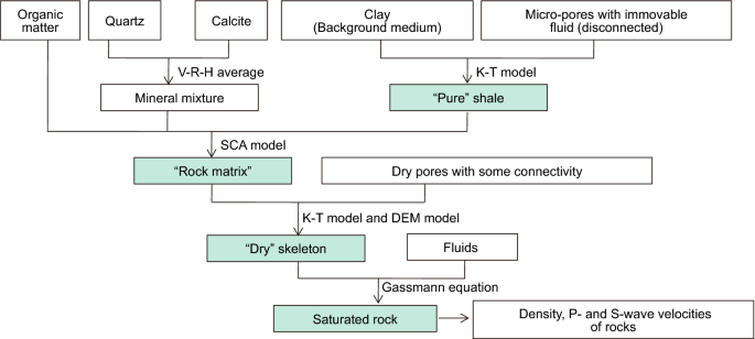
The flowchart of constructed shale rock physics model

2.6 Model test
The input parameters of the constructed shale rock physics model in this paper mainly include: (1) the volume fraction, elastic moduli, and density of each component of shale matrix minerals (quartz, calcite, and clay); (2) the content of organic matter; (3) shale porosity, fluid saturation, elastic moduli, density, and other information.
A well A in a shale gas work area is used to test the constructed shale rock physics model. We use the rock physics model to calculate P- and S-wave velocities of well A and then compare the results with the well log data to verify the reliability and applicability of this model.
Table 1 gives the elastic moduli and density parameters of shale mineral components and filling fluids. Figure 2 shows the well log data of clay content, quartz content, calcite content, TOC content, porosity, and water saturation obtained from the logging interpretation of well A. Figure 3 shows the estimated results of P- and S-wave velocities, and P-to-S-wave velocity ratio.

The comparison of P- and S-wave velocities and P-to-S-wave velocity ratio estimated by shale rock physics model with well log data of well A. aP-wave velocity and estimation errors; b S-wave velocity and estimation errors; cP-to-S-wave velocity ratio and estimation errors

Well log interpretation of clay content, quartz content, calcite content, organic matter content, porosity, and water saturation of well A
From Fig. 3a, b, we can see that the P- and S-wave velocities calculated by the shale rock physics model are in good agreement with the well log data. Moreover, the estimated P-to-S-wave velocity ratio also agrees well with the true logs. The relative errors are very small and almost less than 10%. The marked area indicates the target reservoir and the estimated P- and S-wave velocities decrease in this target area.
3 Brittleness analysis of high-porosity shale gas-bearing reservoir
Due to the low-permeability characteristic of shale, the most effective way to improve the shale gas productivity is the artificial fracturing. Study found that in the same condition of geodynamic background, rock mineralogical compositions and mechanical properties, shale with high contents of organic matter and quartz is more brittle and easier to form natural and induced fractures under the action of tectonic stress in shale rocks. This is conducive to the gathering and seepage of shale gas (Jiang et al. 2010; Ding et al. 2012). Moreover, the fractures produced by fracturing and the fracture network formed by primary pores and micro-fractures in shale gas-bearing reservoir both play a role in storage and migration of shale gas. Therefore, the high porosity of shale plays a positive role in the effect of artificial fracturing. In addition, the area with high gas content is undoubtedly the target location of high gas production in shale gas-bearing reservoirs. To sum up, the region with high porosity, high organic matter content, and high brittle mineral content is the sweet spot of shale reservoirs with high brittleness.
Generally speaking, Young’s modulus (\( E \)) and Poisson’s ratio (\( \upsilon \)) are the most commonly used parameters to characterize the brittleness of rock. Greiser and Bray (2007) propose the shale brittleness index expression based on Young’s modulus (\( E \)) and Poisson’s ratio (\( \upsilon \)), which can be expressed as
where \( V_{\text{P}} \), \( V_{\text{S}} \), and \( \rho \) represent the P- and S-wave velocities, and density, respectively; \( E_{\hbox{max} } \) and \( E_{ \hbox{min} } \) represent the maximum and minimum of Young’s modulus (\( E \)) of rocks; \( \upsilon_{\hbox{max} } \) and \( \upsilon_{\hbox{min} } \) represent the maximum and minimum of Poisson’s ratio (\( \upsilon \)) of rocks; \( BI \) represents the brittleness index of rocks, which is the average of the sum of \( E_{\text{brittleness}} \) and \( \upsilon_{\text{brittleness}} \).
Young’s modulus (\( E \)) indicates the stiffness of rocks, which also known as the stiffness modulus. The greater the value is, the greater the stiffness of rock is. Because the harder shales are better at fracturing than tough shales, they increase the permeability of the area. Therefore, Young’s modulus (\( E \)) is usually used as an important index for the measurement of rock brittleness. Poisson’s ratio (\( \upsilon \)) can be used to characterize the transverse deformation intensity of rocks. The higher its value is, the more prone it is to transverse deformation of rocks. Generally, the reservoir area with high Young’s modulus (\( E \)), low Poisson’s ratio (\( \upsilon \)), and high brittleness index (\( BI \)) is the sweet spot of shale brittleness (Goodway et al. 2010; Sharma and Chopra 2012).
However, it is found that the sensitivity of Young’s modulus (\( E \)) to shale brittleness is reduced by factors such as shale organic matter, porosity, and fluid (see Sect. 3.1 for details). Therefore, Young’s modulus (\( E \)) cannot be fully applied to the indication of brittleness of high gas shale with high TOC content and high porosity under certain circumstances.
The first and second Lamé constants (\( \lambda \) and \( \mu \)) are related to the compressibility and rigidity of rocks and can improve the sensitivity to pore fluids and lithologic changes, further improving the effective identification of reservoir areas (Goodway 2001). According to the analysis of hydrocarbon content and brittleness properties of Texas Barnett shale, Goodway et al. (2010) propose the areas of high Young’s modulus (\( E \)), high first Lamé constants (\( \lambda \)) or Lamé impedance (\( \lambda \rho \)) and low Poisson’s ratio (\( \upsilon \)) to be the high shale gas-bearing reservoirs. Combining the brittleness analysis of high gas shale in this work area, we propose a new brittleness indicator—\( {E \mathord{\left/ {\vphantom {E \lambda }} \right. \kern-0pt} \lambda } \), namely the ratio of Young’s modulus (\( E \)) to the first Lamé constants (\( \lambda \)). Meanwhile, similar to the expression of shale brittleness index based on Young’s modulus (\( E \)) and Poisson’s ratio (\( \upsilon \)) proposed by Greiser and Bray (2007), we propose a new shale brittleness index (\( BI_{\text{NEW}} \)) based on new brittleness indicator (\( {E \mathord{\left/ {\vphantom {E \lambda }} \right. \kern-0pt} \lambda } \)) and Poisson’s ratio (\( \upsilon \)), which can be expressed as
where \( \left( {{E \mathord{\left/ {\vphantom {E \lambda }} \right. \kern-0pt} \lambda }} \right)_{\hbox{max} } \) and \( \left( {{E \mathord{\left/ {\vphantom {E \lambda }} \right. \kern-0pt} \lambda }} \right)_{\hbox{min} } \) represent the maximum and minimum of new brittleness indicator (\( {E \mathord{\left/ {\vphantom {E \lambda }} \right. \kern-0pt} \lambda } \)) of rocks; \( BI_{\text{NEW}} \) represents the new brittleness index of rocks, which is the average of the sum of \( \left( {{E \mathord{\left/ {\vphantom {E \lambda }} \right. \kern-0pt} \lambda }} \right)_{\text{brittleness}} \) and \( \upsilon_{\text{brittleness}} \).
Because the area of high porosity, high brittleness, and high gas reservoir can be regarded as the sweet spot of shale gas-bearing reservoirs, we analyze the effects of quartz, porosity, organic matter, and pore fluids to these five parameters of brittleness indicator, including Young’s modulus (\( E \)), Poisson’s ratio (\( \upsilon \)), brittleness index (\( BI \)), new brittleness indicator (\( {E \mathord{\left/ {\vphantom {E \lambda }} \right. \kern-0pt} \lambda } \)), and new brittleness index (\( BI_{\text{NEW}} \)).
3.1 Model analysis of brittleness parameters
Firstly, we analyze the influence of brittle minerals (quartz) and porosity on these five parameters, such as Young’s modulus (\( E \)), Poisson’s ratio (\( \upsilon \)), brittleness index (\( BI \)), new brittleness indicator (\( {E \mathord{\left/ {\vphantom {E \lambda }} \right. \kern-0pt} \lambda } \)), and new brittleness index (\( BI_{\text{NEW}} \)).
It is assumed that the matrix minerals of rocks only contain quartz (its bulk modulus and shear modulus are 36.6 GPa and 45.0 GPa, respectively) and clay (its bulk modulus and shear modulus are 21.0 GPa and 7.0 GPa, respectively), and the rocks are fully saturated with gas (its bulk modulus and shear modulus of 0.00013 GPa and 0 GPa, respectively). The porosity range of the matrix pores is about 0%–10%. On this basis, the above established rock physics model of shale rocks is used to analyze the influence of quartz content and porosity on Young’s modulus (\( E \)), Poisson’s ratio (\( \upsilon \)), brittleness index (\( BI \)), new brittleness indicator (\( {E \mathord{\left/ {\vphantom {E \lambda }} \right. \kern-0pt} \lambda } \)), and new brittleness index (\( BI_{\text{NEW}} \)), and the results are shown in Fig. 4a–e, in which the different lines represent the different quartz content.

The influence of quartz content and porosity on Young’s modulus (\( E \)), Poisson’s ratio (\( \upsilon \)), brittleness index (\( BI \)), new brittleness indicator (\( {E \mathord{\left/ {\vphantom {E \lambda }} \right. \kern-0pt} \lambda } \)), and new brittleness index (\( BI_{\text{NEW}} \)). a Young’s modulus (\( E \)); b Poisson’s ratio (\( \upsilon \)); c brittleness index (\( BI \)); d new brittleness indicator (\( {E \mathord{\left/ {\vphantom {E \lambda }} \right. \kern-0pt} \lambda } \)); e new brittleness index (\( BI_{\text{NEW}} \))
Figure 4a shows that Young’s modulus (\( E \)) increases with the increase in quartz content and the decrease in porosity. Therefore, Young’s modulus (\( E \)) in the high-porosity shale areas is less sensitive to the brittle minerals (quartz). Figure 4b shows that Poisson’s ratio (\( \upsilon \)) decreases with the increase in quartz content and decreases rapidly with the increase in porosity when the porosity of rock matrix is greater than 4%. Therefore, Poisson’s ratio (\( \upsilon \)) in the high-porosity shale areas is more sensitive to the brittle minerals (quartz). Figure 4c shows that the new brittleness indicator (\( {E \mathord{\left/ {\vphantom {E \lambda }} \right. \kern-0pt} \lambda } \)) increases with the increase in quartz content and the rapid increase in porosity when the porosity of rock matrix is greater than 6%. Moreover, the change range of new brittleness indicator (\( {E \mathord{\left/ {\vphantom {E \lambda }} \right. \kern-0pt} \lambda } \)) is more than Poisson’s ratio (\( \upsilon \)). Therefore, the new brittleness indicator (\( {E \mathord{\left/ {\vphantom {E \lambda }} \right. \kern-0pt} \lambda } \)) in the high-porosity shale area is the most sensitive to brittle minerals (quartz). It can be seen from the comparison between Fig. 4d, e that the quartz content has no correlation with the brittleness index (\( BI \)) and the new brittleness index (\( BI_{\text{NEW}} \)). The new brittleness index (\( BI_{\text{NEW}} \)) increases monotonously with the increase in porosity, but the brittleness index (\( BI \)) decreases first and then increases slowly with the increase in porosity. In summary, the new brittleness index (\( BI_{\text{NEW}} \)) is more sensitive to high-porosity shale areas.
Secondly, we analyze the influence of organic matter content and fluid types on these five parameters, such as Young’s modulus (\( E \)), Poisson’s ratio (\( \upsilon \)), brittleness index (\( BI \)), new brittleness indicator (\( {E \mathord{\left/ {\vphantom {E \lambda }} \right. \kern-0pt} \lambda } \)), and new brittleness index (\( BI_{\text{NEW}} \)).
It is assumed that the matrix minerals of rocks contain organic matter (its bulk modulus and shear modulus are 2.9 GPa and 2.7 GPa, respectively) and clay (its bulk modulus and shear modulus are 21.0 GPa and 7.0 GPa, respectively), and the range of the organic matter is about 0%–25%. The rocks are fully saturated with gas (its bulk modulus and shear modulus are 0.00013 GPa and 0 GPa, respectively) or water (its bulk modulus and shear modulus are 2.25 GPa and 0 GPa, respectively). On this basis, the above established rock physics model of shale rocks is used to analyze the influence of organic matter content and fluid types on Young’s modulus (\( E \)), Poisson’s ratio (\( \upsilon \)), brittleness index (\( BI \)), new brittleness indicator (\( {E \mathord{\left/ {\vphantom {E \lambda }} \right. \kern-0pt} \lambda } \)), and new brittleness index (\( BI_{\text{NEW}} \)), and the results are shown in Fig. 5a–e, in which the different lines represent the different fluid types.

The influence of organic matter content and fluid types on these five parameters, such as Young’s modulus (\( E \)), Poisson’s ratio (\( \upsilon \)), brittleness index (\( BI \)), new brittleness indicator (\( {E \mathord{\left/ {\vphantom {E \lambda }} \right. \kern-0pt} \lambda } \)), and new brittleness index (\( BI_{\text{NEW}} \)). a Young’s modulus (\( E \)); b Poisson’s ratio (\( \upsilon \)); c brittleness index (\( BI \)); d new brittleness indicator (\( {E \mathord{\left/ {\vphantom {E \lambda }} \right. \kern-0pt} \lambda } \)); e new brittleness index (\( BI_{\text{NEW}} \))
Figure 5a, b shows that Young’s modulus (\( E \)) and Poisson’s ratio (\( \upsilon \)) reduce with the increase in organic matter content, and the water-saturated shale has lower values of Young’s modulus (\( E \)) and Poisson’s ratio (\( \upsilon \)) than gas-saturated shale. Therefore, the high value of Young’s modulus (\( E \)) is less sensitive to the gas-bearing shales with high organic matter content. Figure 5c shows that the new brittleness indicator (\( {E \mathord{\left/ {\vphantom {E \lambda }} \right. \kern-0pt} \lambda } \)) increase with the increase in organic matter content, and the gas-saturated shale has high value of new brittleness indicator (\( {E \mathord{\left/ {\vphantom {E \lambda }} \right. \kern-0pt} \lambda } \)) than the water-saturated shale. Therefore, the new brittleness indicator (\( {E \mathord{\left/ {\vphantom {E \lambda }} \right. \kern-0pt} \lambda } \)) is more sensitive to the shales with high organic matter content. Moreover, it can be seen from Fig. 5d, e that the shale brittleness index (\( BI \)) first decreases and then increases with the increase in organic matter content, and the variation range is very small. In contrast, the new brittleness index (\( BI_{\text{NEW}} \)) is more sensitive to the shales with high organic matter content.
In summary, compared with Young’s modulus (\( E \)) and brittleness index (\( BI \)), the new brittleness indicator (\( {E \mathord{\left/ {\vphantom {E \lambda }} \right. \kern-0pt} \lambda } \)) and new brittleness index (\( BI_{\text{NEW}} \)) are more sensitive to the sweet spot of shales with high quartz content, high organic matter content, high porosity, and high gas content.
3.2 Case study
3.2.1 Cross-plots analysis
We use two sets of real data from different work areas to analyze Young’s modulus (\( E \)) and the new brittleness indicator (\( {E \mathord{\left/ {\vphantom {E \lambda }} \right. \kern-0pt} \lambda } \)) by cross-plots, and Figs. 6 and 7 show the results.

Cross-plot of Young’s modulus (\( E \)) and the new brittleness indicator (\( {E \mathord{\left/ {\vphantom {E \lambda }} \right. \kern-0pt} \lambda } \))

Cross-plot of Young’s modulus (\( E \)) and the new brittleness indicator (\( {E \mathord{\left/ {\vphantom {E \lambda }} \right. \kern-0pt} \lambda } \))
From Fig. 6, it can be seen that compared with Young’s modulus (\( E \)), the new brittleness indicator (\( {E \mathord{\left/ {\vphantom {E \lambda }} \right. \kern-0pt} \lambda } \)) is more effective to separate the ductile shale from brittle sandstone, and the gas-bearing sandstone has a higher value of the new brittleness indicator (\( {E \mathord{\left/ {\vphantom {E \lambda }} \right. \kern-0pt} \lambda } \)) than water-bearing one, so it is easy to separate them (dividing line 1). But it is difficult to separate the ductile shale and sandstone containing different fluids by Young’s modulus (\( E \)). So the new brittleness indicator (\( {E \mathord{\left/ {\vphantom {E \lambda }} \right. \kern-0pt} \lambda } \)) comes out as a superior attribute for the estimation of rock brittleness and fluids.
The data in Fig. 7 are the well log data from Mannville region (Goodway 2001), in which the porosity of gas-bearing glauconitic sandstone and gas-bearing lithic sandstone is about 15%–25% and 10%–18%, respectively. It can be observed from horizontal axis that the data of gas-bearing sandstone and background shale are partially overlap, and cannot be distinguished well by using Young’s modulus (\( E \)). However, the new brittleness indicator (\( {E \mathord{\left/ {\vphantom {E \lambda }} \right. \kern-0pt} \lambda } \)) can distinguish gas-bearing sandstone and the background shale obviously (dividing line). In addition, for glauconitic sandstone with larger porosity and lithic sandstone with smaller porosity, the new brittleness indicator (\( {E \mathord{\left/ {\vphantom {E \lambda }} \right. \kern-0pt} \lambda } \)) can also differentiate to some extent. But if Young’s modulus (\( E \)) as the indicative factor, brittleness of lithic sandstone is higher than glauconitic sandstone, which obviously does not agree with the actual situation.
3.2.2 Well log data analysis
Using the same well log data set of well A that was used to do model test above, Young’s modulus (\( E \)), Poisson’s ratio (\( \upsilon \)), brittleness index (\( BI \)), new brittleness indicator (\( {E \mathord{\left/ {\vphantom {E \lambda }} \right. \kern-0pt} \lambda } \)) and new brittleness index (\( BI_{\text{NEW}} \)) are compared and analyzed.
From Fig. 8a, it can be seen that Young’s modulus (\( E \)) has low value in the background ductile shale and gas-bearing brittle shale, while it has high value in sand-shale interbedding and carbonate rock formation. Combining the well log interpretation of Fig. 8b with rock physics analysis above, it is found that in the background ductile shale section, the rock exhibits apparently ductile and Young’s modulus (\( E \)) is low due to its high clay content and low quartz content. In sand-shale interbedding, Young’s modulus (\( E \)) has a high value because of the increase in quartz content and the low contents of porosity, fluids, and organic matter. In gas-bearing shale section, high quartz content can increase Young’s modulus (\( E \)), but the high value of organic content, porosity and gas content reduce it. Therefore, the comprehensive effects of all these factors reduce the sensitivity of Young’s modulus (\( E \)) to quartz content, and the result shows low value. In carbonate rock section, the contents of carbonate minerals (calcite, dolomite, etc.) are high, and contents of quartz, organic matter, pore are low, so the value of Young’s modulus (\( E \)) is high. While Poisson’s ratio (\( \upsilon \)) shows high values in the background ductile shale section, intermediate values in the sand-shale interbedding and carbonate rock formation, and low values in gas-bearing sandstone section. In background shale section, the new brittleness indicator (\( {E \mathord{\left/ {\vphantom {E \lambda }} \right. \kern-0pt} \lambda } \)) shows low values. But in sand-shale interbedding and carbonate rock section, it shows immediate values, and in gas-bearing sandstone section, it shows high values. Similarly, we find that in the background shale section, the value of new brittleness indicator (\( {E \mathord{\left/ {\vphantom {E \lambda }} \right. \kern-0pt} \lambda } \)) is low due to the high clay content and low quartz content and the result is consistent with Young’s modulus (\( E \)). In sand-shale interbedding, porosity and organic matter content are low and the new brittleness indicator (\( {E \mathord{\left/ {\vphantom {E \lambda }} \right. \kern-0pt} \lambda } \)) increases but Poisson’s ratio (\( \upsilon \)) decreases with the increase in the quartz content. In gas-bearing shales, the high values of quartz content, organic matter content, porosity and gas content all enhance the new brittleness indicator (\( {E \mathord{\left/ {\vphantom {E \lambda }} \right. \kern-0pt} \lambda } \)) and reduce Poisson’s ratio (\( \upsilon \)); therefore, the new brittleness indicator (\( {E \mathord{\left/ {\vphantom {E \lambda }} \right. \kern-0pt} \lambda } \)) has the maximum value, and Poisson’s ratio (\( \upsilon \)) shows the minimum value. In carbonate rock section, because the carbonate minerals (calcite, dolomite, etc.) have some brittleness and high content, the values of the new brittleness indicator (\( {E \mathord{\left/ {\vphantom {E \lambda }} \right. \kern-0pt} \lambda } \)) and Poisson’s ratio (\( \upsilon \)) are medium.

Parameter curves of well A. a Parameter curves of Young’s modulus (\( E \)), Poisson’s ratio (\( \upsilon \)), brittleness index (\( BI \)), new brittleness indicator (\( {E \mathord{\left/ {\vphantom {E \lambda }} \right. \kern-0pt} \lambda } \)), and new brittleness index (\( BI_{\text{NEW}} \)); b well log interpretation of quartz content, organic matter content, porosity, and water saturation
The shale brittleness index (\( BI \)), which combines Young’s modulus (\( E \)) and Poisson’s ratio (\( \upsilon \)), has high values in sand-shale interbedding and carbonate rock sections, immediate values in gas-bearing shales, and low values in background shale section. However, the new brittleness index (\( BI_{\text{NEW}} \)), which combines the new brittleness indicator (\( {E \mathord{\left/ {\vphantom {E \lambda }} \right. \kern-0pt} \lambda } \)) and Poisson’s ratio (\( \upsilon \)), has the largest values in gas-bearing shales, medium values in sand-shale interbedding section, and low values in background shale section. Moreover, the values of each section show obvious differences.
From the analysis of Young’s modulus (\( E \)), Poisson’s ratio (\( \upsilon \)), brittleness index (\( BI \)), new brittleness indicator (\( {E \mathord{\left/ {\vphantom {E \lambda }} \right. \kern-0pt} \lambda } \)) and new brittleness index (\( BI_{\text{NEW}} \)), it is known that Young’s modulus (\( E \)) is a good indicator only for the compact sandstone and cannot obviously characterize gas-bearing brittle rock because of the negative impact of its high contents of organic matter, porosity and gas, while the new brittleness indicator (\( {E \mathord{\left/ {\vphantom {E \lambda }} \right. \kern-0pt} \lambda } \)) can characterize gas-bearing brittle rocks better. Besides quartz content, the new brittleness indicator (\( {E \mathord{\left/ {\vphantom {E \lambda }} \right. \kern-0pt} \lambda } \)) is also sensitive to the comprehensive effects of organic matter, porosity, and fluids. So this factor has better guiding significance for the selection of fracturing area of shale gas-bearing reservoirs.
4 Conclusions
In this study, based on the comprehensive analysis of shale gas-bearing reservoir, we propose a new process of shale rock physics model to estimate the P- and S-wave velocities. The trial result shows that the estimated velocities are in good agreement with the well log data.
We use the constructed rock physics model to make the analysis of the brittleness of organic-rich shale gas-bearing reservoirs, and propose a new brittleness indicator (\( {E \mathord{\left/ {\vphantom {E \lambda }} \right. \kern-0pt} \lambda } \)). Compared with the conventional brittleness indicator of Young’s modulus (\( E \)), the new brittleness indicator (\( {E \mathord{\left/ {\vphantom {E \lambda }} \right. \kern-0pt} \lambda } \)) is more sensitive to the high brittle shales with high organic matter content, high porosity, and high gas content, which can be used to better indicate the sweet spot of shale gas-bearing reservoirs. Moreover, compared with the conventional shale brittleness index (\( BI \)) based on Young’s modulus (\( E \)) and Poisson’s ratio (\( \upsilon \)), the new shale brittleness index (\( BI_{\text{NEW}} \)) based on the new brittleness indicator (\( {E \mathord{\left/ {\vphantom {E \lambda }} \right. \kern-0pt} \lambda } \)) and Poisson’s ratio (\( \upsilon \)) is more sensitive to the characterization of high-porosity shale gas-bearing reservoirs. Therefore, the combination of the new brittleness indicator (\( {E \mathord{\left/ {\vphantom {E \lambda }} \right. \kern-0pt} \lambda } \)), Poisson’s ratio (\( \upsilon \)), and new shale brittleness index (\( BI_{\text{NEW}} \)) can better indicate the strong fracturing zone of shale gas-bearing reservoirs.
References
Alzate JH, Devegowda D. Integration of surface seismic, microseismic, and production logs for shale gas characterization: methodology and field application. Interpretation. 2013;1(2):SB37–49. https://doi.org/10.1190/int-2013-0025.1.
Ba J, Yan XF, Chen ZY, et al. Rock physics model and gas saturation inversion for heterogeneous gas reservoirs. Chin J Geophys. 2013;56(5):1696–706. https://doi.org/10.6038/cjg20130527(in Chinese).
Bandyopadhyay K, Sain R, Liu E, et al. Rock property inversion in organic-rich shale: uncertainties, ambiguities, and pitfalls. SEG Tech Program Expand Abstr. 2012. https://doi.org/10.1190/segam2012-0932.1.
Bayuk IO, Ammerman M, Chesnokov EM. Upscaling of elastic properties of anisotropic sedimentary rocks. Geophys J Int. 2008;172:842–60. https://doi.org/10.1111/j.1365-246x.2007.03645.x.
Berryman JG. Long-wavelength propagation in composite elastic media. Acoust Soc Am. 1980;68:1809–31. https://doi.org/10.1121/1.385171.
Berryman JG. Mixture theories for rock properties. In: Ahrens TJ, editor. Rock physics and phase relations, a handbook of physical constants. Washington, DC: American Geophysical Union; 1995. p. 205–28. https://doi.org/10.1029/rf003p0205.
Budiansky B. On the elastic moduli of some heterogeneous materials. J Mech Phys Solids. 1965;13:223–7. https://doi.org/10.1016/0022-5096(65)90011-6.
Chen JJ, Zhang GZ, Chen HZ, et al. The construction of shale rock physics effective model and prediction of rock brittleness. SEG Tech Program Expand Abstr. 2014. https://doi.org/10.1190/segam2014-0716.1.
Ding WL, Li C, Li CY, et al. Dominant factor of fracture development in shale and its relationship to gas accumulation. Earth Sci Front. 2012;19(2):212–20 (in Chinese).
Dong DZ, Zou CN, Li JZ, et al. The resource potential and exploration prospect of shale gas. Geol Bull China. 2011;30(2–3):324–36 (in Chinese).
Fu YQ, Ma FM, Zeng LX. The key technology of shale gas reservoir fracturing experiments evaluation. Nat Gas Ind. 2011;31(4):51–4 (in Chinese).
Gassmann F. Über die Elastizitat poröser Medien. Vier.der Natur. Geselschaft in Zürich. 1951;96:1–23.
Goodway B. AVO and Lamé constants for rock parameterization and fluid detection. CSEG Rec. 2001;6:39–60.
Goodway B, Perez M, Varsek J, et al. Seismic petrophysics and isotropic-anisotropic AVO methods for unconventional gas exploration. Lead Edge. 2010;29(12):1500–8. https://doi.org/10.1190/1.3525367.
Grieser W, Bray J. Identification of production potential in unconventional reservoir. SPE production and operations symposium, SPE. 2007;10662. https://doi.org/10.2118/106623-ms.
Hill R. A self-consistent mechanics of composite materials. J Mech Phys Solids. 1965;13:213–22. https://doi.org/10.1016/0022-5096(65)90010-4.
Hornby BE, Schwartz LM, Hudson JA. Anisotropic effective-medium modeling of the elastic properties of shales. Geophysics. 1994;59:1570–83. https://doi.org/10.1190/1.1443546.
Jiang WL, Zhao SP, Zhang JC, et al. The comparison of main controlling factors between coalbed methane and shale gas gathering. Nat Gas Geosci. 2010;2(6):1057–60 (in Chinese).
Keys RG, Xu SY. An approximation for the Xu-White velocity model. Geophysics. 2002;67:1406–14. https://doi.org/10.1190/1.1512786.
King MS. Rock-physics developments in seismic exploration: a personal 50-year perspective. Geophysics. 2005;70(6):3–8. https://doi.org/10.1190/1.2107947.
Li WG, Yang SL, Yin DD, et al. A review of shale gas development technology and strategy. Nat Gas Oil. 2011;29(1):34–7 (in Chinese).
Li QH, Chen M, Jin Y, et al. Rock mechanical properties and brittleness evaluation of shale gas reservoir. Pet Drill Tech. 2012;40(4):17–22 (in Chinese).
Liu ZS, Sun ZD. New brittleness indexes and their application in shale/clay gas reservoir prediction. Pet Explor Dev. 2015;42(1):129–37. https://doi.org/10.1016/s1876-3804(15)60016-7.
Liu C, Fu W, Guo ZQ, et al. Rock physics inversion for anisotropic shale reservoirs based on Bayesian scheme. Chin J Geophys. 2018;61(6):2589–600. https://doi.org/10.6038/cjg2018L0176(in Chinese).
Ma SF, Han DK, Gan LD, et al. A review of seismic rock physics models. Prog Geophys. 2010;25(2):460–71 (in Chinese).
Mavko G, Mukerji T, Dvorkin J. The rock physics handbook tools for seismic analysis of porous media. 2nd ed. New York: Cambridge University Press; 2009.
Nie HK, Zhang JC. Types and characteristics of shale gas reservoir: a case study of Lower Paleozoic in and around Sichuan Basin. Pet Geol Exp. 2011;33(2):219–32 (in Chinese).
Pan XP, Zhang GZ, Yin XY. Estimation of effective geostress parameters driven by anisotropic stress and rock physics models with orthorhombic symmetry. J Geophys Eng. 2017;14:1124–37. https://doi.org/10.1088/1742-2140/aa6f6b.
Pan XP, Zhang GZ, Yin XY. Seismic scattering inversion for anisotropy in heterogeneous orthorhombic media. Chin J Geophys. 2018a;61(1):267–83. https://doi.org/10.6038/cjg2018K0609(in Chinese).
Pan XP, Zhang GZ, Yin XY. Probabilistic seismic inversion for reservoir fracture and petrophysical parameters driven by rock-physics models. Chin J Geophys. 2018b;61(2):683–96. https://doi.org/10.6038/cjg2018K0759(in Chinese).
Pan XP, Zhang GZ. Amplitude variation with incident angle and azimuth inversion for Young’s impedance, Poisson’s ratio, and fracture weaknesses in shale gas reservoirs. Geophys Prospect. 2019;67:1898–911. https://doi.org/10.1111/1365-2478.12783.
Perez R, Marfurt K. Brittleness estimation from seismic measurements in unconventional reservoirs: application to the Barnett Shale. SEG Tech Program Expand Abstr. 2013. https://doi.org/10.1190/segam2013-0006.1.
Qian KR, Zhang F, Chen SQ, et al. A rock physics model for analysis of anisotropic parameters in a shale reservoir in Southwest China. J Geophys Eng. 2016;13:19–34. https://doi.org/10.1088/1742-2132/13/1/19.
Qian KR, He ZL, Chen YQ, et al. Prediction of brittleness based on anisotropic rock physics model for kerogen-rick shale. Appl Geophys. 2017;14(4):463–79. https://doi.org/10.1007/s11770-017-0640-y.
Ruppel SC, Loucks RG. Black mudrocks: lessons and questions from the Mississippian Barnett Shale in the southern Midcontinent. Sediment Rec. 2008;6(2):4–8. https://doi.org/10.2110/sedred.2008.2.4.
Sharma RK, Chopra S. New attribute for determination of lithology and brittleness. SEG Technical Program Expanded Abstracts, 2012;10:45–7. https://doi.org/10.1190/segam2012-1389.1.
Wang ZJ. Fundamentals of seismic rock physics. Geophysics. 2001;66(2):398–412. https://doi.org/10.1190/1.1444931.
Wang X, Liu YH, Zhang M, et al. The study of shale gas forming conditions and affecting factors. Nat Gas Geosci. 2010;21(2):350–5 (in Chinese).
Wu X, Chapmann M, Li XY, et al. Anisotropic elastic modeling for organic shales. EAGE Tech Program Expand Abstr. 2012. https://doi.org/10.3997/2214-4609.20148651.
Xu S, Payne MA. Modeling elastic properties in carbonate rocks. Lead Edge. 2009;28:66–74. https://doi.org/10.1190/1.3064148.
Yu BS. Particularity of shale gas reservoir and its evaluation. Earth Sci Front. 2012;19(3):252–8 (in Chinese).
Zhang GZ, Chen JJ, Chen HZ, et al. Prediction for in situ formation stress of shale based on rock physics equivalent model. Chin J Geophys. 2015a;58(6):2112–22. https://doi.org/10.6038/cjg20150625(in Chinese).
Zhang GZ, Pan XP, Sun CL, et al. Seismic fluid identification using a nonlinear elastic impedance inversion method based on a fast Markov chain Monte Carlo method. Pet Sci. 2015b;12:406–16. https://doi.org/10.1007/s12182-015-0046-5.
Zhu Y, Xu S, Payne M, et al. Improved rock-physics model for shale gas. SEG Tech Program Expand Abstr. 2012. https://doi.org/10.1190/segam2012-0927.1.
Author information
Authors and Affiliations
Corresponding author
Additional information
Edited by Jie Hao
Rights and permissions
Open Access This article is licensed under a Creative Commons Attribution 4.0 International License, which permits use, sharing, adaptation, distribution and reproduction in any medium or format, as long as you give appropriate credit to the original author(s) and the source, provide a link to the Creative Commons licence, and indicate if changes were made. The images or other third party material in this article are included in the article's Creative Commons licence, unless indicated otherwise in a credit line to the material. If material is not included in the article's Creative Commons licence and your intended use is not permitted by statutory regulation or exceeds the permitted use, you will need to obtain permission directly from the copyright holder. To view a copy of this licence, visit http://creativecommons.org/licenses/by/4.0/.
About this article

Cite this article
Pan, XP., Zhang, GZ. & Chen, JJ. The construction of shale rock physics model and brittleness prediction for high-porosity shale gas-bearing reservoir. Pet. Sci. 17, 658–670 (2020). https://doi.org/10.1007/s12182-020-00432-2
Received:
Published:
Issue Date:
DOI: https://doi.org/10.1007/s12182-020-00432-2