


1. Introduction
The Greenland Ice Sheet (GrIS) has experienced mass loss during the past several decades (e.g. Mankoff and others, Reference Mankoff2019; Mouginot and others, Reference Mouginot2019) and studies indicate that one of the primary drivers of mass loss is the surface mass balance (SMB) (e.g. van den Broeke and others, Reference van den Broeke2016). Given that accumulation rates vary in response to several decadal climatic oscillations such as the North Atlantic Oscillation and the Atlantic Multi-decadal Oscillation (e.g. Andersen and others, Reference Andersen2006; Lenaerts and others, Reference Lenaerts, Medley, van den Broeke and Wouters2019), it is important to establish if SMB rates and patterns have changed in the past, either spatially (e.g. the pattern has changed) or temporally (the accumulation rates have changed). One way to extend accumulation records back in time is to use accumulation reconstructed from ice cores (e.g. Buchardt and others, Reference Buchardt, Clausen, Vinther and Dahl-Jensen2012; Rasmussen and others, Reference Rasmussen2013). However, ice-core records are spatially sparse and represent point measurements. Thus, ice-core records struggle to disentangle a signal resulting from a change in SMB pattern from a signal resulting from a change in SMB rate. An interpretation of accumulation rates from ice cores must therefore take into account that an apparent change in accumulation rate may be a shift in accumulation pattern rather than a (direct) climate signal.
The radioglaciological community has in recent decades employed ice-penetrating radar to close this gap in knowledge. The underlying assumption of the radioglaciological approach is that the internal layers observed in radar data are isochrones (cf. Eisen and others, Reference Eisen2008) and that their depth depends primarily on surface accumulation and densification rates. The first examples of studies deriving accumulation rates in this way include ground-based radar data from Antarctica (Richardson and others, Reference Richardson, Aarholt, Hamran, Holmlund and Isaksson1997) and airborne radar data from Greenland (Dahl-Jensen and others, Reference Dahl-Jensen1997). With the advent of NASA's (National Aeronautics and Space Administration, USA) airborne Operation IceBridge (OIB) mission, the community gained access to spatially extensive radar data, leading to efforts focusing on large-scale mapping of the layers (Karlsson and others, Reference Karlsson, Dahl-Jensen, Gogenini and Paden2013; MacGregor and others, Reference MacGregor2015) and assessments of the state of the firn (Forster and others, Reference Forster2013). Importantly, the range of frequencies employed by OIB has allowed for the retrieval of accumulation rates over different time-scales including annual accumulation rates (Koenig and others, Reference Koenig2016, Montgomery and others, Reference Montgomery, Koenig, Lenaerts and Kuipers Munneke2020), decadal averages for the past 40 years (Medley and others, Reference Medley2013), decadal to centennial averages over the past several hundred years (Karlsson and others, Reference Karlsson2016; Lewis and others, Reference Lewis2017) and Holocene-average values (Nielsen and others, Reference Nielsen, Karlsson and Hvidberg2015; MacGregor and others, Reference MacGregor2016).
While the spatially extensive data coverage from the airborne campaigns have returned numerous important insights, the spatially confined ground-based surveys can in turn yield information with higher spatial resolution within targeted areas. Examples include data acquired by Hawley and others (Reference Hawley2014) during a traverse from Thule, North Greenland, to Summit Station, data collected by Miège and others (Reference Miège2013) from a high accumulation area in Southeast Greenland and a recent study by Lewis and others (Reference Lewis2019) using data from West Greenland. One area that may specifically benefit from the increased resolution of a ground-based survey is the region around major ice divides. The location of the ice divide exerts an important control on accumulation rates in northern Greenland since it acts as a topographic barrier for atmospheric transport of water vapour (Ohmura and Reeh, Reference Ohmura and Reeh1991). Studies have shown that this results in high accumulation rates west of the ice divide, and very dry conditions east of the ice divide (e.g. Bales and others, Reference Bales, McConnell, Mosley-Thompson and Csatho2001; Box and others, Reference Box2013; Lenaerts and others, Reference Lenaerts, Medley, van den Broeke and Wouters2019). The gradient in accumulation rates may be very steep in this region (cf. Karlsson and others, Reference Karlsson2016) making ground-based radar data particularly useful. Furthermore, the sensitivity of the accumulation rate to the ice divide location is important for the interpretation of ice-core records, since ice cores are typically drilled on the ice divide.
In this study, we make use of radar data collected by ground-based receivers during two traverses along the ice divide of the GrIS and in the northeastern sector. We trace the internal layers in the data and date them by transferring an already established age–depth relationship (Karlsson and others, Reference Karlsson2016) to our dataset. In order to infer the accumulation rates, we then employ inverse modelling, a well-known approach to retrieving information from radar layers using, for example, a Metropolis algorithm (e.g. Buchardt and Dahl-Jensen, Reference Buchardt and Dahl-Jensen2007; Steen-Larsen and others, Reference Steen-Larsen, Waddington and Koutnik2010; Karlsson and others, Reference Karlsson2016) or gradient-type methods (e.g. Waddington and others, Reference Waddington, Neumann, Koutnik, Marshall and Morse2007; Nielsen and others, Reference Nielsen, Karlsson and Hvidberg2015). We are thus able to extract spatially dense and temporally well-resolved accumulation rates with a high spatial resolution. In our case, we use a 200 m grid along the radar survey lines.
2. Data
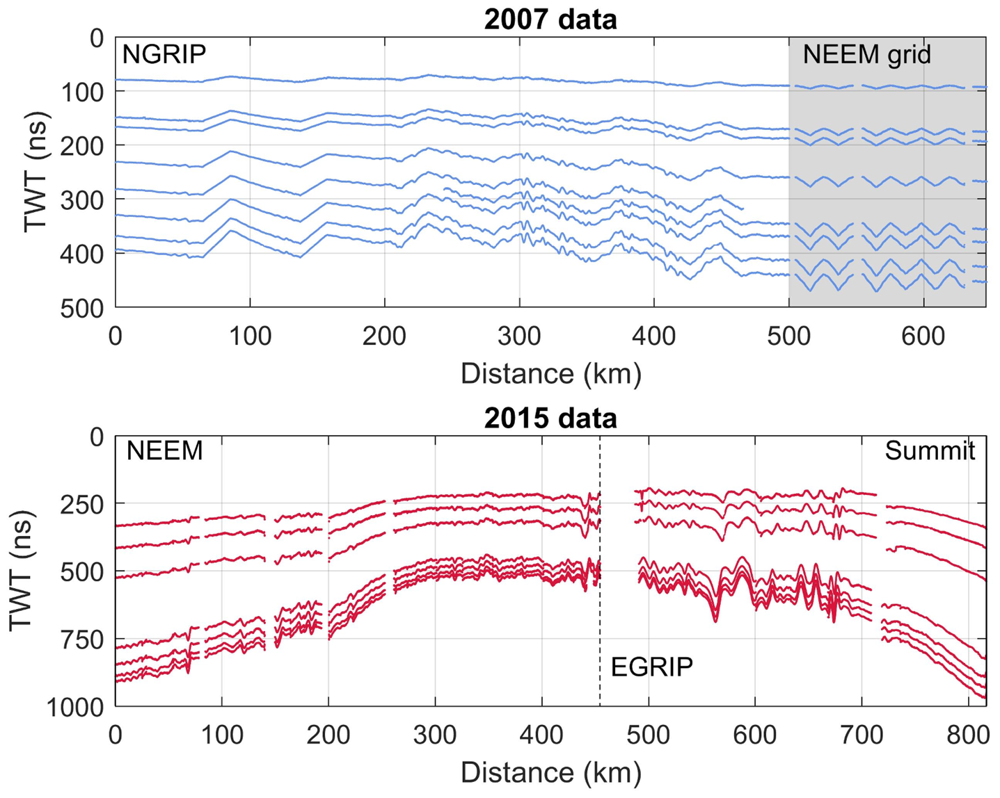
The area investigated in this study is located within the dry-snow zone in northern Greenland (Fig. 1). The radar data were collected in connection with two traverses where scientific investigations were carried out alongside logistical efforts to relocate substantial camp equipment. During both field seasons, the radar data were collected with a RAMAC GPR (Malå Geosciences, Sweden) with a shielded antenna. In 2007, a centre frequency of 250 mHz was used, while in 2015, two shielded antennas were deployed with centre frequencies of 250 and 500 mHz. All the traced layers are shown in Figure 2. In this study, we focus on the data from the 250 mHz antenna.

Fig. 1. (A and B) Maps of survey areas and ground-based radar data lines. Field stations are marked with red circles. The 2007 survey route is in blue and the 2015 survey route in red. (C) Layout of the NEEM grid (blue) and location of the radargrams shown in Figure 3 from the ground-based 2015 AWI data and the airborne 2011 OIB survey.
In addition to the ground-based datasets, we use radar data acquired by the Center for Remote Sensing of Ice Sheets (CReSIS) as part of OIB in the vicinity of NEEM (North Greenland Eemian Ice Drilling) in 2011. This dataset serves as a guideline for layer dating.
2.1. Data acquisition 2007
During the summer season of 2007, a joint Danish–American–German surface traverse travelled from NGRIP (North Greenland Ice Core Project, 75.1°N, 42.3°W, 2957 m a.s.l.) to NEEM (77.5°N, 51.0°W, 2481 m a.s.l.) (Fig. 1B, blue line). The route followed the ice divide in a northern and north-western direction. A team from the Alfred Wegener Institute (AWI), Germany, performed high-resolution GPR measurements along the route resulting in a radar profile with a length of 607 km. In addition, a survey consisting of a grid with dimensions of 10 km × 10 km and a line spacing of 1 km was carried out around the planned drilling location at NEEM (Fig. 1C). The total length of the radar lines in the grid is ~120 km. The received radar signals were recorded within a time window of 502 ns (~50 m depth) with 1024 vertical samples. During data acquisition, horizontal twofold stacking was performed, while the shot distance was triggered by an odometer wheel every 1 m.
The GPR surveys were supplemented by kinematic GPS (Global Positioning System) measurements with two receivers: a Trimble 4000 SSI, operating at 1 Hz, and a NovAtel OEM-4, operating at 20 Hz. The raw GPS data are, therefore, equidistant in time but not in space due to varying travelling velocity of the snowmachine, usually between 4 and 5 m s−1.
2.2. Data acquisition 2015
In summer 2015, a Danish–German traverse team travelled from NEEM to EGRIP (East Greenland Ice Core Project, 75.64°N, 36°W, 2712 m a.s.l.) and a smaller team continued to Summit (72.58°N, 38.46°W, 3250 m a.s.l.) (Fig. 1B, red line). Part of the route retraced the 2007 traverse along the ice divide but then veered towards the east. Between NEEM and EGRIP, the data were collected from snowmachine with a travel speed between 2.5 and 3 m s−1 with a horizontal spacing between signals of ~1 m triggered by an odometer wheel. An example of a radargram acquired with this configuration is shown in Figure 3A. Between EGRIP and Summit, the data collection was carried out from a KAS tractor with the antennas resting on a high-molecular weight polyethylene sled. The travel speed was significantly higher (~4 m s−1) and the horizontal spacing between signals was therefore increased to 2 m, also triggered by an odometer wheel. For both parts of the survey, the received signals were recorded within a time window of 1142 ns (about 110 m depth) with 2048 vertical samples. The distance between antennae and snowmobile was several metres, and the distance between antennae and KAS tractor was more than 10 m. We did not observe any interference from either vehicle with the radar signal. During data acquisition, horizontal eightfold stacking was performed. The total length of collected GPR data was 820 km.

Fig. 3. Radargram from the ground-based 2015 data (A) where the numbers in the radargram title indicate acquisition date and line number, and the airborne 2011 data (B) where the numbers in the radargram title indicate acquisition date, line number and subset of line. The circles show the layers matched by visual inspection. In the airborne data, dashed lines show the layers that were traced and dated by Karlsson and others (Reference Karlsson2016). The dashed lines in the ground-based data (A) indicate the internal layers that were traced in this study. Diamonds indicate the seven layers in the ground-based data transferred to the airborne data.
3. Methods
In the following, we detail how the observed two-way travel time (TWT) of the internal layers is converted to accumulation rates. The underlying assumption of this method is that the layers represent isochrones. We also assume that their depth is primarily determined locally by densification, past accumulation rates and layer thinning caused by ice flow. We do not include the influence of horizontal advection. Furthermore, we assume that accumulation rates are equivalent to the net local specific SMB.
3.1. Layer tracing and depth-conversion
In the 2007 data, the internal layers were picked using the seismic-software package OpenWorks (application SeisWorks2D) from the producer Landmark. By using the semi-automatic picking tool, seven layers could be determined. In the 2015 data, the layers were traced manually in the seismic software package epos/ECHOS (cf. Fig. 2). Only moderate processing was applied to the data, mainly sevenfold horizontal stacking and modest filtering to decrease noise, namely, a Butterworth filter with cut-off frequencies of 200 and 350 MHz, respectively, and an automatic gain control.
The depth of the layers is recorded in TWT by the receiver. The signal propagation velocity v of radar waves in firn as a function of depth z depends on the ordinary relative permittivity ɛ′ of the firn,

where c 0 is the speed of light in vacuum. We assume that the relative permittivity is related to the density of the firn through the real-valued Looyenga mixing model (Looyenga, Reference Looyenga1965)

where ρ i is the density of ice ρ i = 917 kg m −3, and ρ is the depth-dependent density of the firn. We specify below how we obtain the depth-dependent density. We use a value for the relative permittivity of ice of ɛ′i = 3.15 (Eisen and others, Reference Eisen, Wilhelms, Steinhage and Schwander2006; Bohleber and others, Reference Bohleber, Wagner and Eisen2012).
3.2. Age assignment
We use the age–TWT relationship established by Karlsson and others (Reference Karlsson2016) for an airborne radar dataset from OIB. In the following, we will refer to this age–TWT relationship as the K16-dating. We transfer the K16-dating to our datasets in the following way: In the Karlsson and others (Reference Karlsson2016) study, measurements of density and dielectric properties of the shallow core NEEM11S1 were used as input for a model of electromagnetic wave propagation in ice (‘emice’, Eisen and others, Reference Eisen, Wilhelms, Steinhage and Schwander2006). The shallow core was drilled less than a few hundred metres from the main NEEM core. The ‘emice’ model produces a synthetic radargram and converts the core's depth-scale to TWT. By matching the synthetic radargram with dated volcanic horizons (e.g. Sigl and others, Reference Sigl2013) a relationship between age and TWT was established. A radargram from the OIB data with traced layering is shown in Figure 3B. We use this age–TWT relationship to assign ages to our observed radar layers. This transfer is not straightforward as the airborne data were collected in 2011, while the ground-based data are from 2007 and 2015. First, we consider our 2015 data. This dataset was acquired 4 years after the OIB data and has thus been subjected to 4 years of accumulation and corresponding downwards movement during that time. When we attempt to pinpoint the OIB layers in our 2015 data, we therefore expect the layers to be buried deeper in the firn. In contrast, the 2007 data are 4 years older than the OIB data, and the internal layers are therefore expected to be found higher up in the firn column compared to the 2011 data.
The first assessment of the layer age is based on a visual inspection of the radar data. We use radar lines acquired at NEEM that are spatially close to each other (all radar datasets had acquisitions in this area). It should be noted that due to differences in radar systems, this manual matching is prone to errors. For example, multiple layers in the ground-based data may appear as a single layer in the airborne data because of different bandwidths and antenna settings and thus different vertical resolution. We therefore aim to identify similar layer packages (patterns of high/low reflection strengths) in the two radar lines in addition to individual layers.
The second method for transferring the age–TWT relationship is based on theoretical considerations of changes in layer depth over time. In this approach, we calculate a theoretical offset in TWT based on simple assumptions of firn density and accumulation rates. The relationship between age and depth is determined by the layer thinning due to ice flow and firn densification. The layer thinning from ice flow can be described as a decreasing linear function. This assumption breaks down in deep ice, however, in the shallow part that we consider here it as (depths shallower than 150 m) a reasonable assumption. We base this assertion on the fact that in our study area, the characteristic lengths associated with changes in accumulation rates or ice thicknesses are one to two orders of magnitude larger than the longest particle path, indicating that local accumulation rates dominate layer depths (cf. Waddington and others, Reference Waddington, Neumann, Koutnik, Marshall and Morse2007). The layer thinning is described by the vertical velocity w as

where $\dot {b}_{\rm i}$ is the accumulation rate in metre ice equivalents, H is ice thickness and $\hat {z}$
 is the depth in ice metre equivalent (cf. Nye, Reference Nye1957; Dansgaard and Johnsen, Reference Dansgaard and Johnsen1969). This depth scale must be converted from ice metre to true depth using the density of the firnpack. Here, we assume that the density can be described as an exponential function (Cuffey and Paterson, Reference Cuffey and Paterson2010):

where ρ i is the density of ice, ρ s is the density of the surface snow and C is a constant. Note that here z is in true depth. Since the density increases with depth, a layer deposited on the surface will thin as it densifies and move downwards in the firn column even in the absence of ice flow. In the following, we assume that the densification rate is constant in time even if the accumulation rate varies. Lacking detailed density measurements along the traverse route, we construct a mean density profile from multiple measured densities in central Greenland (see Bolzan and Strobel, Reference Bolzan and Strobel1994; Wilhelms, Reference Wilhelms1996; Schwager, Reference Schwager2000). We also calculate the standard deviation of this combined record. We then use this information to get a first estimate of $\dot {b}_{\rm i}$ and the parameters in Eqn (4) that we can use in our age assignment and as a first guess in the inverse model (see below).
3.3. Solving the inverse problem
Converting the observed TWT of the internal layers to accumulation rates is a typical inverse problem: We have a model described by Eqns (1–4), and we have a number of unknown parameters; the surface density ρ s, the densification rate C and the accumulation rate $\dot {b}_{\rm i}$ . Typically, an inverse problem is described as Aster and others (Reference Aster, Borchers and Thurber2013): m = g−1(d), where ${\bf m} \in {\opf R}^N$
 is a set of model parameters, ${\bf d}\in {\opf R}^M$
 is the observable data and g is a vector operator called the forward operator. The calculated model parameters are evaluated based on the misfit between the observed and the modelled observables. We solve the inverse problem using a Monte Carlo method. Following Mosegaard and Tarantola (Reference Mosegaard and Tarantola1995), we explore the parameter space randomly and accept or reject model parameters based on the Metropolis criterion (see Appendix for more information on the inverse method). In our case, the data are depths of the internal layers in TWT and their age. The forward operator describes the vertical movement downwards in the firn column for some given accumulation and densification.
The layer tracing results in very high horizontal resolution depth-information (order of 1 m at the NEEM site) – much higher resolution than what we are able to resolve with the inverse method, and also higher resolution than the expected variability in accumulation rate. We therefore resample the data to 200 m horizontal resolution. We then define our parameter space, i.e. the range of values that constrain the model parameters. Since the data were acquired in low accumulation areas as well as high accumulation areas, we set the allowed accumulation range to 0.05 to 0.4 m a−1 ice equivalent in order to capture the entire range of possible values. In the following, all accumulation rates will be in m a−1 ice equivalent (using ρ i = 918 kg m −3). We base the parameters for the densification rate (Eqn (4)) on the density measurements from northern and central Greenland (Bolzan and Strobel, Reference Bolzan and Strobel1994; Wilhelms, Reference Wilhelms1996; Schwager, Reference Schwager2000). This gives an average surface density of the upper 2 m ranging from 331 to 363 kg m−3 with a mean of 354 kg m−3. The C-parameter is based on the bestfit of Eqn (4) to the density measurements and from this, the allowed range is between 0.025 and 0.0305 m−1 with a mean of 0.0278 m−1.
Because the deepest layer is the least sensitive to errors in density, depth or age, we first apply the inverse method to the deepest layer only. We then apply our inverse algorithm using all the layers, and use the calculated accumulation rate from the deepest layer to drive the initial guess, retrieving the average annual accumulation rate since time of deposition of the oldest layer and time of radar acquisition.
4. Results
4.1. Age assignment
The visual inspection of the 2015 data and the OIB data led to the identification of tenmatching layers or layer packages in both radargrams (Fig. 3, circles). The offset in TWT between the match points varies between 6 and 23 ns with a mean of 14.4 ns. We compare these values to the theoretical offset between the layering in the two datasets calculated from Eqns (3–4). We use the following constants in order to calculate the theoretical offset in TWT over 4 years at NEEM: $\dot {b}_{{\rm i\comma NEEM}} = 0.23\, {\rm m\, a}^{-1}$ , H NEEM = 2800 m, ρi,NEEM = 917 kg m −3, C NEEM = 0.0263 m−1 and ρs,NEEM = 340 kg m −3. As expected, the offset is larger for shallower layers. At 100 ns it is 14 ns while in the 300–1000 ns range the offset is close to constant for all depths: ~12 ns over 4 years.
Based on these results, we transfer the dating of the layers. We further find that three of the layers that are traced in the 2015 data are likely identical to layers traced in the OIB data (cf. Fig. 3). The age–TWT relationship is summarized in Table 1. The deepest layer is assigned an age of 321 years, thus the results from the inverse model will give us the annual average accumulation rate over a 321-year period. Given uncertainties in firn density and the resolution of the radar signal, we estimate the measurement error to be of the order of 15 ns which corresponds approximately to 5 years (at NEEM).
Table 1. Year of deposition and age of traced layers in the 2015 data

The layers traced in the 2007 data are located at shallower depths (between ~100 and 500 ns) compared to the layers traced in the 2015 data (between ~250 and 1000 ns, cf. Fig. 2). Using the theoretical consideration outlined above (Eqns (3–4)), we get an offset ranging between 14 ns for the uppermost layer and 11.4 ns for the deepest layer. That is, in the 2007 data, the traced layers are expected to be 11.4–14 ns higher up in the firn column compared to the OIB data. Using this offset, we are again able to assign an age to the layers by transferring the K16-dates to the layers (see Table 2). Here, the oldest layer is assigned an age of 150 years, and we are therefore able to retrieve 150-year average accumulation rates from this dataset.
Table 2. Year of deposition and age of traced layers in the 2007 data
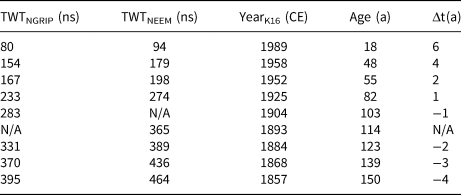
Notes: Δt is the difference in age between the K16-dating and the NGRIP-dating. Layers that do not reach an ice-core site are denoted N/A.
As an additional check on the assigned ages, we compare the K16-dating to the age–depth relationship from the NGRIP core from 2003. This age–depth relationship was established by Vinther and others (Reference Vinther2006) and we refer to it as the NGRIP-dating. We assume that the relationship is constant in time (i.e. that accumulation rates, densification and layer thinning are constant), since studies have shown that large variations in accumulation rates did not take place during most of the latter part of the Holocene (Vinther and others, Reference Vinther2006; Karlsson and others, Reference Karlsson2016). Thus, we can calculate the expected age of the traced layers by converting their TWT to depth using the same densification description as above. The results can be seen in Table 2. The mean difference in ages of the layers t between the two age–depth relationships is

where N is number of layers at NGRIP. The absolute mean is 2.9 years, and the shallowest layer has the largest discrepancy (6 years) likely due to the fact that its depth is more sensitive to the inaccuracies in assumed density. Note that the K16-dating predicts older ages than the NGRIP-dating for the deep layers but younger ages for the shallower layers (cf. Table 2).
4.2. Accumulation rates from 2007 survey
Figure 4A shows the 150-year average accumulation rates during the period 1857–2007 CE reconstructed from the 2007 survey. On the 200 m resolution output, the accumulation rates range from 0.15 to 0.26 m a−1 with a mean of 0.21 m a−1 and a standard deviation of 0.02 m a−1. The results indicate two spatial trends. Firstly, there is a minimum in accumulation rates approximately halfway between NGRIP–NEEM and the highest accumulation rates are found in the area around NEEM. Secondly, there is a spatial variability in the east–west direction with a clear contrast between the north-eastern side of the ice divide and the south-western side. When the traverse route enters the eastern side of the ice divide, accumulation rates decrease.
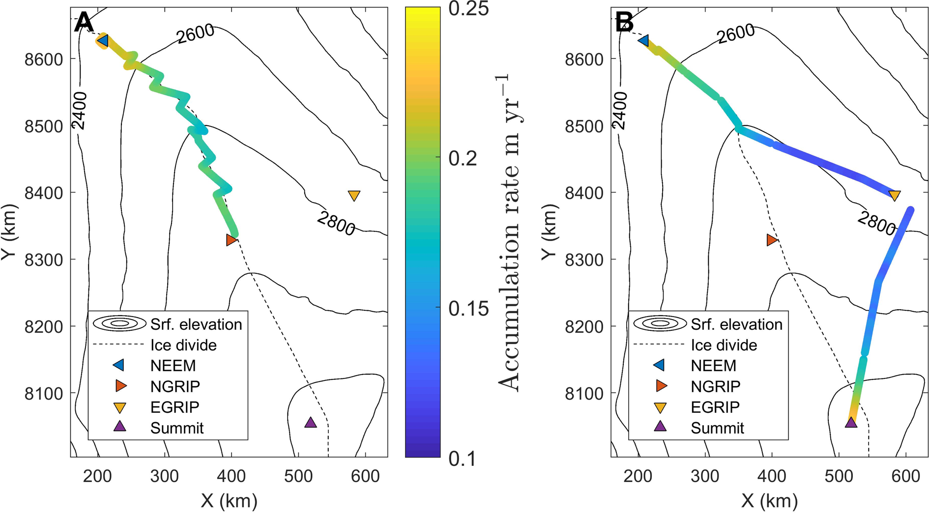
Fig. 4. (A) Mean accumulation rates 1857–2007 CE from the 2007 traverse (smoothed with 5 km running mean). (B) Mean accumulation rates 1694–2015 CE from the 2015 traverse (smoothed with 5 km running mean). Surface elevation is from Bamber and others (Reference Bamber, Layberry and Gogineni2001).
Figure 5A shows the accumulation rate plotted with distance along the radar profiles. Here, the variations in the 150-year average accumulation rates along the traverse are clearly visible (black line); the undulations along the profile for the 2007 survey correspond to where the traverse route moved laterally across the ice divide. This variation is still visible when the data are smoothed with a 5 km moving window. In the figure, the yellow shading indicates the accumulation rates retrieved from individual layer depths, i.e. over shorter time scales. Our inverse formulation does not have enough information to constrain the accumulation rates for the individual layers. This is because in each point we attempt to retrieve not just accumulation rates but also the three parameters relating to the density, implying that if we were to retrieve accumulation rates from individual layers, we would be attempting to infer four parameters from a single data point. This lack of information manifests itself as a large spread in the resulting accumulation rates, and therefore we do not sub-divide our accumulation rates into shorter time segments.
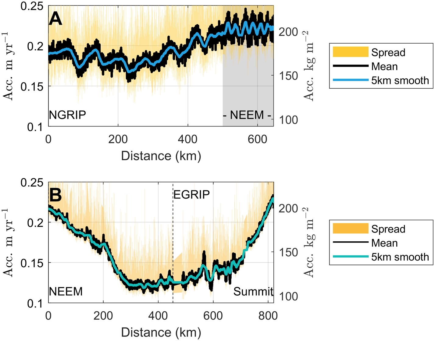
Fig. 5. Accumulation rates along the 2007 traverse (A) and 2015 traverse (B). The labelled ice-core sites are at the end points of the figure except for EGRIP where the location of the station is indicated with a dashed black line. The shaded grey area indicates the gridded data that were collected around NEEM at the end of the 2007 traverse. Black line indicates the retrieved average accumulation, blue line is the smoothed accumulation rate over a 5 km moving average, and the yellow shading shows the spread in retrieved accumulation rates for each individual radar layer.
The change in accumulation from west to east is further investigated by interpolating our inversely modelled accumulation rates onto a 200 m grid extending 10 km to either side of the ice divide. We then define four lines that cross the ice divide perpendicularly, and extract the accumulation rates along those lines from the gridded map. This returns the general trend in accumulation rate across the divide but due to the interpolation any small-scale variations (~ <1 km) will not be captured. The results are shown in Figure 6. The steepest gradient is found in the southern part with a change in accumulation of ~1 mm a−1 km−1. In contrast, the lower-elevation area towards NEEM has no distinct accumulation gradient. All lines display some undulations which may be related to redistribution of snow around the topographic high that coincides with the ice divide.
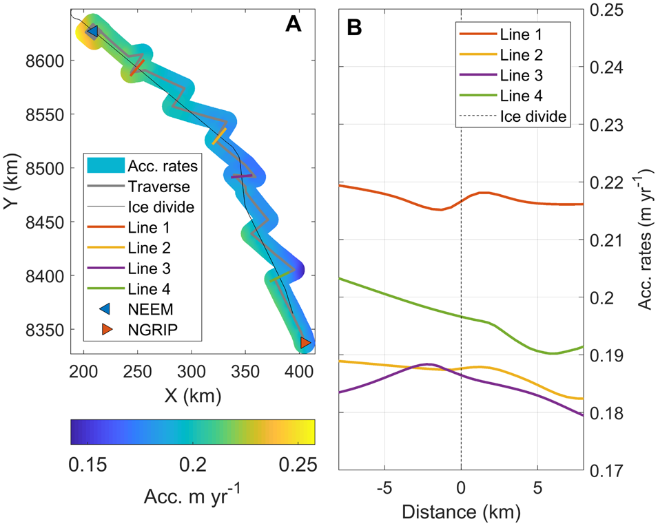
Fig. 6. (A) Gridded accumulation rates 1857–2007 CE from the 2007 traverse. (B) Interpolated accumulation rates 1857–2007 CE from the 2007 traverse across the ice divide.
4.3. Accumulation rates from 2015 survey
The 321-year average accumulation rates from the period 1694–2015 CE reconstructed from the 2015 data can be seen in Figure 4B. In the 200 m resolution output, the accumulation rate ranges from 0.11 to 0.23 m a−1 with a mean of 0.16 m a−1 and a standard deviation of 0.04 m a−1. The results show distinct spatial trends: In the part of the traverse route that follows the ice divide, the accumulation rates decrease as surface elevation increases. When the route diverts from the ice divide towards the east, the accumulation rates decrease further. Finally, as the route approaches Summit Station, accumulation rates increase again and reaches values similar to those found at NEEM. Note that the gradient in accumulation rate is steep in both cases, estimated at 0.8 mm a−1 km−1. This is of a similar scale as the gradient across the ice divide reported above for the 2007 survey but over a substantially larger spatial scale. Another noteworthy spatial variability is the large undulation to higher and then lower accumulation rates ~550 km from NEEM (Fig. 5B). This area is outside the fast-flowing North East Greenland Ice Stream so the radar layers are not expected to be modified by contemporary ice dynamics.
Similar to the 2007 data, our inverse formulation does not have enough information to retrieve accumulation rates from individual radar layers. We therefore only report on the 321-year average accumulation rates. In Figure 5B, the yellow shading shows the spread in these individual accumulation rates.
4.4. Comparison with firn and ice core measurements
We compare our radar-derived accumulation rates with those derived from measurements of firn and ice cores. The three main data sources are (1) the accumulation rates reconstructed from the deep ice cores GISP2 (Greenland Ice Sheet Project 2), NGRIP and NEEM (using data published by Alley, Reference Alley2000; Andersen and others, Reference Andersen2006; Rasmussen and others, Reference Rasmussen2013, respectively), (2) the firn cores collected during the PARCA (Program for Arctic Regional Climate Assessment) campaigns and summarized by Bales and others (Reference Bales, McConnell, Mosley-Thompson and Csatho2001, Reference Bales2009) and (3) the ice cores drilled during the NGT (North Greenland Traverse) where accumulation rates have been reconstructed by Weißbach and others (Reference Weißbach2016). We note that the datasets do not always overlap in time and interpretations of the comparisons should bear this in mind. The location of the cores and their derived accumulation rates are shown in Figure 7. Details on the individual differences between accumulation rates from this study and from the cores can be found in the Appendix Table B1 along with information on location and temporal span of each core. In summary, our accumulation rates deviate <5% from the accumulation rates found from the deep ice cores and 10% or less from the cores from NGT and PARCA. The good agreement between our results and the accumulation rates measured in the firn cores gives us further confidence in our results.
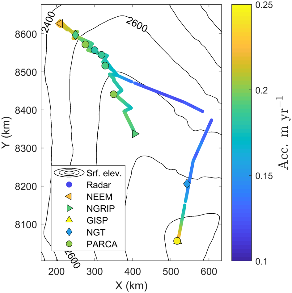
Fig. 7. Radar-derived accumulation rates and accumulation rates from firn and ice cores (cf. Table B1 in Appendix).
Accumulation rates are not yet available from the EGRIP core but Vallelonga and others (Reference Vallelonga2014) report an annual layer thickness of 0.11 m during the past ~400 years. This is lower than our accumulation rate of 0.13 m a−1 (during 1694–2015); however, annual layer thicknesses are not equivalent to accumulation rates, since layer thinning is not taken into account and accumulation rates are thus expected to be higher than the observed annual layer thicknesses.
5. Discussion
5.1. Uncertainties
The uncertainty of the results is the combined effect of uncertainties related to our method (uncertainties due to assumptions in our forward and inverse models, e.g. how well the densification rate is captured, the fact that we neglect horizontal ice-flow) and uncertainties introduced by, for example, errors in layer tracing and dating. Karlsson and others (Reference Karlsson2016) used the same methodology as presented here, and we therefore base our discussion of uncertainties on their findings. Firstly, they found that the treatment of the densification rate had negligible influence on the uncertainty of the results. Similarly, the overall effect of neglecting horizontal ice flow was found to be small when internal layers are relatively shallow (as they are here). Generally, if a snow particle is deposited in a low accumulation area and then travels towards a high accumulation area, our model will underestimate the accumulation rate. The opposite applies for particles travelling from high to low accumulation areas. Using balance velocities and the present-day spatial variability of accumulation rates (Burgess and others, Reference Burgess2010), we estimate that this over/underestimation is two orders of magnitude lower than the accumulation rates. The overall effect is an underestimation of the spatial variability of the accumulation rates. Our data were acquired in slow flowing areas (velocities below 10 m a−1 for 90% of data points), thus the layers are unlikely to have moved very far from their place of deposition. In our study, the deepest layers is 321-year old, and based on balance velocities from the area, the furthest that layer could have moved is 25 km (in the region close to EGRIP where velocities are of the order of 100 m a−1). We compare the accumulation rates at the point of deposition with accumulation rates at the end point (using the accumulation rates published by Burgess and others (Reference Burgess2010), see below) and find that the largest discrepancy is 3%, and that more than 65% of the data points have a discrepancy below 1% between point of deposition and end point. Thus, we conclude that neglecting horizontal advection is justified and does not significantly impact our uncertainties. This is in line with conclusions from previous studies (e.g. MacGregor and others, Reference MacGregor2016; Nielsen and others, Reference Nielsen, Karlsson and Hvidberg2015).
The effects of the second group of uncertainties are less easily quantified. Errors in layer dating and tracing will have two separate effects. An error in layer dating would lead to a shift in the accumulation rate but the spatial variability (the accumulation pattern) would still be valid. An error in the layer tracing would also impact the spatial variability. An independent check on the assigned ages can be found by comparing the K16-dating with the NGRIP-dating. We compare the age of the layers dated at NEEM using the K16-dating against the age–depth relationship at NGRIP. Here, we calculate a mean difference in age of <1 year (see Table 1). This corresponds to ~3 ns (see section above on age assignment).
Karlsson and others (Reference Karlsson2016) found that a mistake in layer tracing (e.g. an incorrect layer is traced in part of the dataset) would lead to an abrupt step in the resulting accumulation rate. We do not observe any such sharp transitions in our results but we caution that the inverse routine does impose a degree of smoothness which could mask a small jump. A small offset in layer dating can quickly lead to relatively large discrepancies in the accumulation rates compared with ice-core records (Karlsson and others, Reference Karlsson2016). Considering that our results deviates <5% from GISP2, NEEM and NGRIP, we are confident that we have assigned the correct ages within our uncertainty estimate. The discrepancy between the radar-derived accumulation rates and those from the NGT and PARCA cores are larger (up to 10%) and probably partly related to the difference in time periods covered by the observations. Especially in regards to the PARCA cores, this is not surprising since those cores cover shorter time-scales (<20 years) than the radar data. Karlsson and others (Reference Karlsson2016) found similar discrepancies between their results and the accumulation rates from the NGT and PARCA cores.
Finally, we can also adopt a more pragmatic approach to estimating the uncertainty by simply considering the characteristics of our inversion results. Namely the fact that the results exhibit high-frequency fluctuations that are unlikely to be physical – or if they are a physical feature then they are most likely a result of processes that are not captured in our model. In Figure 5, the fluctuations in our 200 m resolution output (thick black line) is clearly visible when compared to the 5 km smoothed result (blue line). If we consider the difference between the 5 km smoothed accumulation rates and the results with 200 m along-track resolution, we find that 95% of the high-resolution data points differ by 6% or less from the smoothed results. We note that this is similar to the uncertainty assigned in Karlsson and others (Reference Karlsson2016). In view of this and the discrepancies between deep ice-core records and our radar-derived accumulation rates discussed above, we assign an uncertainty of 6% to our accumulation rates.
5.2. Comparison with previous radar studies
We compare our results with results from other studies where accumulation rates have been retrieved from radar data. Figure 8B shows our gridded accumulation rates from 1858–2007 CE (light blue line) interpolated onto a OIB flightline and from the 1694–2015 CE average accumulation rate smoothed with a 5 km moving average (dark blue line). In addition, green lines show the mean accumulation rates along the OIB line for the periods 1611–2011 CE and 1811–2011 CE from Karlsson and others (Reference Karlsson2016), and 1712–2014 CE from Lewis and others (Reference Lewis2017). Bear in mind that the derived accumulation rates do not cover exactly the same locations and time intervals. Nevertheless, there is overall a high degree of agreement between the different observational studies. For example, all results clearly show a dip in accumulation rate ~170 km from NEEM, followed by a slight increase in accumulation and then almost constant accumulation rates from 220 km to NGRIP. The accumulation rates calculated by Lewis and others (Reference Lewis2017) have a tendency to be slightly lower than the results from Karlsson and others (Reference Karlsson2016) (mean average difference is − 0.0043 m a−1, corresponding to $\sim -2\percnt$ ). The accumulation rates from 1694–2015 CE (2015 dataset) are lower than the 1857–2007 CE gridded results (2007 dataset) and also lower than those from Karlsson and others (Reference Karlsson2016), although the differences are not statistically significant. In contrast, a simple t-test shows that the difference between the accumulation rates from Lewis and others (Reference Lewis2017) and the 1694–2015 CE average (2015 dataset) is significantly different with a confidence level of <5%. That is not the case for the difference between the accumulation rates from Lewis and others (Reference Lewis2017) and the 1858–2007 CE average (2007 dataset). All accumulation rates from Karlsson and others (Reference Karlsson2016) and Lewis and others (Reference Lewis2017) fall within our stated uncertainty of 6% (see Fig. B1 in the Appendix for a version with errorbars).

Fig. 8. Comparison between accumulation rates derived from radar data in this study (blue lines) and previous studies (green lines). In addition, outputs from the following regional climate models are included: The Polar MM5 (Fifth Generation Mesoscale Model) modified with observations by Burgess and others (Reference Burgess2010), RACMO2 (Regional Atmospheric Climate Model) from Ettema and others (Reference Ettema2009) and MAR (Modèle Atmosphérique Régionale) from Delhasse and others (Reference Delhasse, Kittel, Amory, Hofer and Fettweis2019).
In spite of the fact that the accumulation rates presented above represent different time periods, there is no significant difference between them. In other words, average accumulation rates during the past 150 years are similar to average accumulation rates during the past 321 years. This leads us to conclude that there have not been any substantial changes in accumulation rates over the covered time period, although our results do not preclude that short (e.g. decadal) temporal variations in accumulation rates have taken place. This also indicates that the ice divide has not changed position during the past ~400 years – or if it has changed position the shift has not been large enough to cause a change in accumulation rate.
5.3. Accumulation rates in larger-scale context
Finally, we compare our results with outputs from several regional climate models, namely, The Polar MM5 (Fifth Generation Mesoscale Model) from Burgess and others (Reference Burgess2010), RACMO2 (Regional Atmospheric Climate Model) from Ettema and others (Reference Ettema2009) and MAR (Modèle Atmosphérique Régionale) from Delhasse and others (Reference Delhasse, Kittel, Amory, Hofer and Fettweis2019). The former incorporates observations into the final model output, while the output from the latter two are model-based. While the model results from Burgess and others (Reference Burgess2010) align well with our radar-derived accumulation rates, the outputs from RACMO2 (Ettema and others, Reference Ettema2009) and MAR (Delhasse and others, Reference Delhasse, Kittel, Amory, Hofer and Fettweis2019) show large differences, and these differences are statistically significant with a confidence level of <1%. In fact, both RACMO2 and MAR underestimate the amount of accumulation compared to our results. This is the case along the ice divide (Fig. 8B) as well as in the northeastern sector (Fig. 9). Comparing the results based on 1694–2015 CE radar layers to the regional-climate-model outputs, we find that discrepancies are especially pronounced here, with both RACMO2 and MAR underestimating accumulation rates by more than 35%. The snow deposition in the climate models is not high enough in this part of the ice sheet and this is problematic for accurate assessments of present-day mass loss. Studies often rely on SMB estimates to obtain the mass budgets for the different sectors of the GrIS (Mankoff and others, Reference Mankoff2019; Mouginot and others, Reference Mouginot2019), and an incorrect distribution of snow deposition will therefore influence this assessment.

Fig. 9. Comparison between accumulation rates from this study (blue line) and regional climate model outputs from: The Polar MM5 (Fifth Generation Mesoscale Model) modified with observations by Burgess and others (Reference Burgess2010), RACMO2 (Regional Atmospheric Climate Model) from Ettema and others (Reference Ettema2009) and MAR (Modèle Atmosphérique Régionale) from Delhasse and others (Reference Delhasse, Kittel, Amory, Hofer and Fettweis2019).
6. Conclusion
Ground-penetrating radar reveals stratigraphic information that may be assumed to be isochronous and thus can be used to retrieve information on past accumulation rates and patterns. Here, we use radar data from two ground-based surveys conducted in the interior of the GrIS in 2007 and 2015. The layers imaged by the radar are dated using information from ice-core records and previous studies. From the dated layers, we retrieve the accumulation rates along the radar lines using an inverse method that incorporates a simple densification function with 1D layer thinning. Our results reveal the large-scale variability of the accumulation rates on centennial averages, namely average rates from 1857–2007 CE and 1694–2015 CE. There is overall good agreement with previous observational studies and accumulation rates reconstructed from firn and ice cores. We detect no differences between the 150 year-average accumulation rates from 1857–2007 CE and the 321-year average accumulation rate from 1694–2015 CE, and we interpret this as a sign of a stable accumulation regime and no ice divide migration over the last three centuries. Comparing with regional climate models, we show that the models significantly underestimate the accumulation rates in the interior of the ice sheet. In the northeastern sector, the model outputs diverge from our results by upwards of 35%.
This study demonstrates how radar-derived accumulation rates may provide important insights into the spatial distribution of accumulation, and thus may serve as benchmarks for climate models as well as informing the ice-core community on the areal context for ice-core measurements.
Reconstructed age–TWT relationships and the derived accumulation rates are available at PANGEA (DOI: 10.1594/PANGAEA.915507 and 10.1594/PANGAEA.915505) or upon request from the authors.
Acknowledgments
We acknowledge the help and support from the NGRIP, NEEM and EGRIP projects. EGRIP is directed and organized by the Centre of Ice and Climate at the Niels Bohr Institute, Copenhagen. It is supported by funding agencies and institutions in Denmark (A. P. Möller Foundation, University of Copenhagen), USA (US National Science Foundation, Office of Polar Programs), Germany (Alfred Wegener Institute, Helmholtz Centre for Polar and Marine Research), Japan (National Institute of Polar Research and Artic Challenge for Sustainability), Norway (University of Bergen and Bergen Research Foundation), Switzerland (Swiss National Science Foundation), France (French Polar Institute Paul-Emile Victor, Institute for Geosciences and Environmental research) and China (Chinese Academy of Sciences and Beijing Normal University). We thank both traverse teams, in particular P. Sperlich who participated in the collection of the 2007 data. We thank Emerson E&P Software, Emerson Automation Solutions, for providing licenses in the scope of the Emerson Academic Program. We also thank X. Fettweiss for making the MAR data files available to us. We are grateful for the comments and suggestions for improvements from two anonymous reviewers and the editor, M. Koutnik.
Appendices
Appendix A: inverse method
We follow Mosegaard and Tarantola (Reference Mosegaard and Tarantola1995) and define the misfit function as

where s i is the uncertainty of data point d i. The error on the data points are assumed to be independent. We need to find the model parameters that minimize this misfit function and we do that by exploring the parameter space. It is most convenient to do this randomly using the Monte Carlo algorithm (Mosegaard and Tarantola, Reference Mosegaard and Tarantola1995) and then accept or reject model parameters based on the Metropolis criterion

If L(mi) ≥ L(mj), the step is accepted. Otherwise the step is accepted with a probability of L(mi)/L(mj). Regardless of the size of the random steps, this Metropolis sampler should eventually converge on the target distribution. One problem with the approach presented above is the size of the step. If the step size is too large, we might overlook a good solution and overstep. If the step size is too small, the inverse method becomes too slow. Ideally, between 30 and 60% of guesses should be accepted, so step size is adjusted for this by trial and error.
Appendix B
TABLE B1. Accumulation rates from ice and firn cores compared to the accumulation rates derived in this study
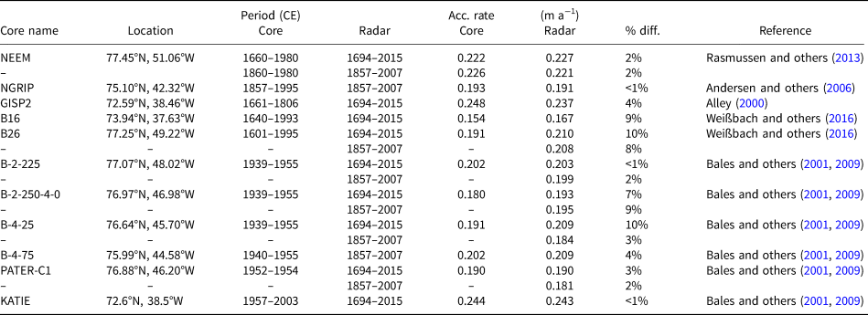
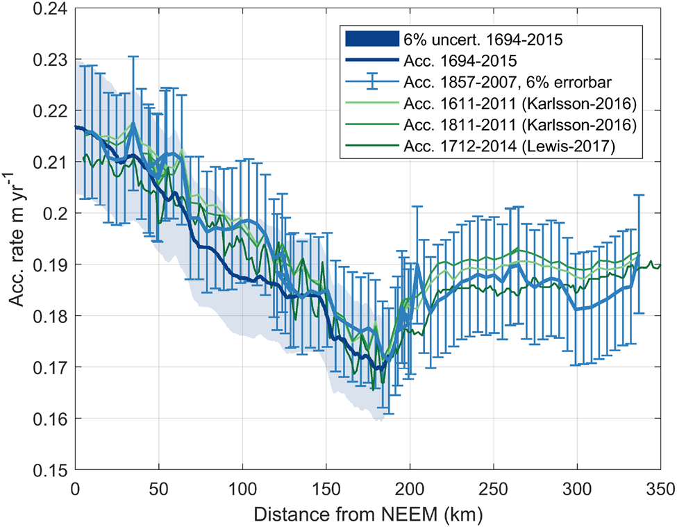
Fig. B1. Comparison between accumulation rates from this study (blue line) and radar-derived accumulation rates from Karlsson and others (Reference Karlsson2016) and Lewis and others (Reference Lewis2017). Errorbars and shading indicate 6% uncertainty.


 Open access