Investigation of Melt Pool Geometry Control in Additive Manufacturing Using Hybrid Modeling


1
Department of Mechanical Engineering, Pennsylvania State University, University Park, PA 16802, USA
2
Department of Mathematics, Pennsylvania State University, University Park, PA 16802, USA
*
Author to whom correspondence should be addressed.
Metals 2020, 10(5), 683; https://doi.org/10.3390/met10050683
Submission received: 4 April 2020
/
Revised: 15 May 2020
/
Accepted: 18 May 2020
/
Published: 22 May 2020
Abstract
:Metal additive manufacturing (AM) works on the principle of consolidating feedstock material in layers towards the fabrication of complex objects through localized melting and resolidification using high-power energy sources. Powder bed fusion and directed energy deposition are two widespread metal AM processes that are currently in use. During layer-by-layer fabrication, as the components continue to gain thermal energy, the melt pool geometry undergoes substantial changes if the process parameters are not appropriately adjusted on-the-fly. Although control of melt pool geometry via feedback or feedforward methods is a possibility, the time needed for changes in process parameters to translate into adjustments in melt pool geometry is of critical concern. A second option is to implement multi-physics simulation models that can provide estimates of temporal process parameter evolution. However, such models are computationally near intractable when they are coupled with an optimization framework for finding process parameters that can retain the desired melt pool geometry as a function of time. To address these challenges, a hybrid framework involving machine learning-assisted process modeling and optimization for controlling the melt pool geometry during the build process is developed and validated using experimental observations. A widely used 3D analytical model capable of predicting the thermal distribution in a moving melt pool is implemented and, thereafter, a nonparametric Bayesian, namely, Gaussian Process (GP), model is used for the prediction of time-dependent melt pool geometry (e.g., dimensions) at different values of the process parameters with excellent accuracy along with uncertainty quantification at the prediction points. Finally, a surrogate-assisted statistical learning and optimization architecture involving GP-based modeling and Bayesian Optimization (BO) is employed for predicting the optimal set of process parameters as the scan progresses to keep the melt pool dimensions at desired values. The results demonstrate that a model-based optimization can be significantly accelerated using tools of machine learning in a data-driven setting and reliable a priori estimates of process parameter evolution can be generated to obtain desired melt pool dimensions for the entire build process.
1. Introduction
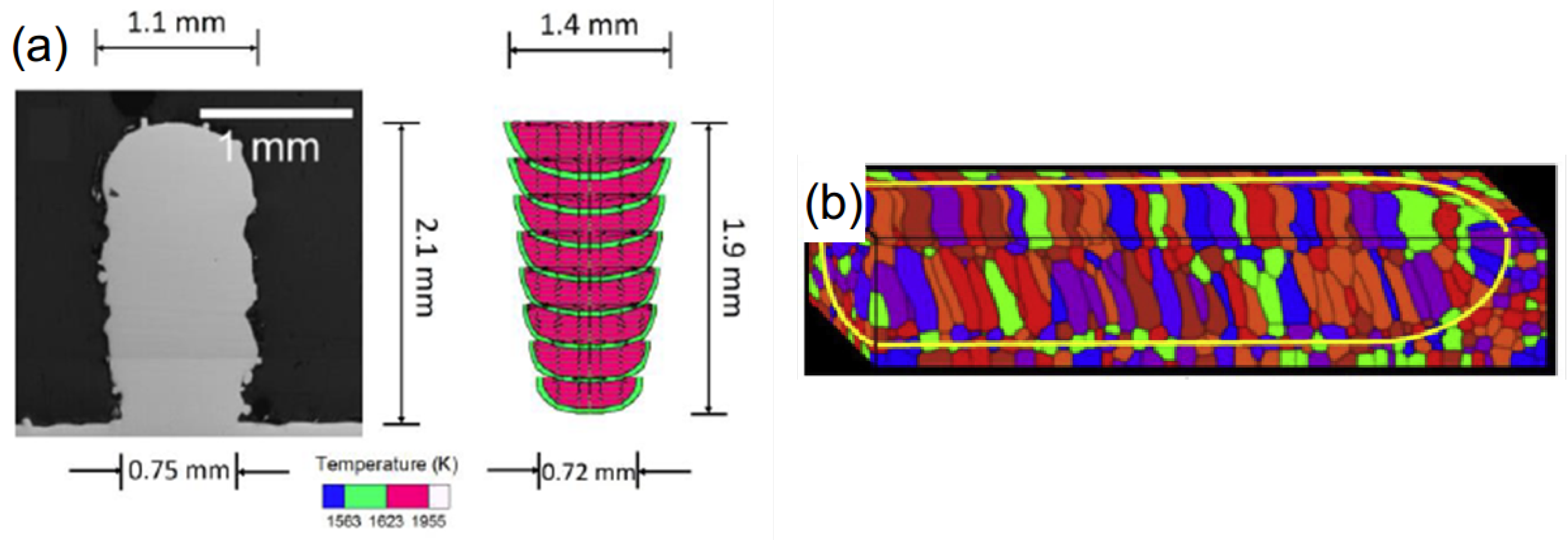
Metal additive manufacturing (AM) facilitates direct fabrication of near-net-shape metallic components, prototypes, or both under rapid solidification conditions [1]. AM is currently used in manufacturing a wide variety of components with increasing complexity, for example, fuel nozzles, rocket injectors, and lattice structures [2]. The concept of AM is built on the principle of incremental layer-by-layer material consolidation through localized melting and resolidification of feedstock materials by using high-power energy sources [3]. The localized heating causes the formation of a melt pool that controls the microstructure and, therefore, the properties of the manufactured component [3]. Due to the cyclic nature of the deposition process as AM components continue to gain thermal energy, the thermal gradient (G) and the solidification velocity (R) inside the melt pool continuously change, resulting in significant alterations in the melt pool properties (e.g., geometry, thermal profile, and flow field among others) between the initial and final layers [4,5] as illustrated in Figure 1a. Figure 1b shows that in spite of fixing the G/R ratio at a value meant for yielding a columnar microstructure, at the leading edge (e.g., beginning of the scan), the grains are columnar; however, at the trailing edge (e.g., towards the end of the scan), the grains become equiaxed [6] due to progressive heating. The primary reason for controlling melt pool geometry in metal AM is to allow a part to be built with consistent melt pool dimensions, even as thermal conditions change continuously [7]. Understanding the fundamental physics of the melt pool evolution is, therefore, a key requirement for AM process development, optimization, and control. Although high-fidelity computational modeling of AM processes can provide reliable estimates of the melt pool evolution during the build process, such elaborate models are nearly-intractable when coupled with an optimization code for melt pool geometry control due to the computational costs [8]. Therefore, while these models are well suited for understanding the physical phenomena, challenges exist in using them for performing process design, optimization, and control [9].
In this respect, machine learning (ML) shows potential in assisting and automating the process of manufacturing [10] through reliable prediction of melt pool geometries [11]. For example, Neural Networks (NN) [12] are widely used as a popular choice in prediction problems by modeling nonparametric input–output relationships. Despite the simplicity of usage, most of these techniques based on complex NN architectures suffer from issues of interpretability [13]. Moreover, the applications of such methods in limited datasets are rare, and lack of data can often result in poor predictive models that lack generalizability due to overfitting [14]. Moreover, a vast majority of the ML techniques used in AM relies on point estimates of the quantities of interest, without catering for uncertainty in the predictions. In critical applications involving high stakes associated with mispredictions, the estimates of uncertainty are particularly important. An attractive alternative, therefore, is to use probabilistic ML techniques like Gaussian Processes (GPs) [15] that offer the advantages of interpretability and applicability in limited data regimes. However, their applications in surrogate-based modeling and optimization are relatively less explored in multi-physics problems in AM. An implementation of surrogate modeling through the construction of computationally efficient approximations that can be used in lieu of the original simulation model [16], therefore, holds significant promise in metal AM.
Surrogate-assisted modeling and optimization techniques are popularly used in various applications that involve expensive computational models [17,18,19,20,21,22,23] for function evaluations. Among the different types of surrogate models, GPs [15] are used profusely for modeling black-box functions whereby a fully Bayesian approach allows for probabilistic estimates of the target functions [24,25,26,27]. With a relatively small number of measurements, a GP surrogate can be learnt to serve as a proxy to an expensive objective function [28] (e.g., prediction of melt pool dimensions for a range of process parameters in metal AM [29]). Under the settings of a GP surrogate, a Bayesian Optimization (BO) set-up can be invoked for gradient-free global optimization of an objective function under budget limitations [30] (e.g., prediction of optimal process parameters for controlling temporal melt pool dimensions in metal AM within N number of iterations; N being an user input). Moreover, with nonlinearities in the objective function, a search for optimum would require significant amount of sampling in the search space, particularly in high dimensions. In such settings, BO is found to be quite successful [31].
In the field of AM, there are very few applications of GPs as surrogate models for expensive experiments and simulations. For example, Tapia et al. [32] used experimental data to learn spatial GPs for predicting porosity in metal AM produced during the laser powder bed fusion process. In another work, Tapia at al. [16] demonstrated the usage of GPs in predicting melt pool depth as a function of different process parameters, which were used to describe regimes of operation where the process was expected to be robust. Seede et al. [33] used a GP framework to develop a calibrated surrogate model for predicting optimal process parameters for building porosity free parts with low-alloy martensitic steel AF9628. However, to the best of the authors’ knowledge, no work exists in the field of AM that leverages the surrogate-based predictions and uses them as a basis for active learning strategies for optimizing a desired objective, e.g., controlling melt pool dimensions over time under computational budget constraints in laser powder bed fusion process. The design and deployment of such predictive methodologies will immensely augment the response time of feedback or feedforward control strategies as the current response times are rather long compared to the process time scales [34].
To address this gap, this paper proposes a novel framework of controlling the melt pool geometry in laser powder bed fusion process by formulating it as an optimization problem through the integration of the tools of physics-based analytical modeling and data-driven analysis. The cardinal contribution of this work in AM is to bridge the gap in model-assisted prediction and control of melt pool geometry by using ML techniques that can potentially accelerate the process of melt pool geometry control. The results demonstrate that by using a low-cost surrogate-assisted modeling using GP and BO, it is possible to obtain an excellent estimation of process parameter evolution as a function of time in order to maintain the desired meltpool geometry (e.g., dimensions) throughout the build process. The framework consists of three critical steps: (i) evaluation of the thermal field using an experimentally validated 3D analytical melt pool evolution model which serves as a source of data for formulating a GP surrogate, (ii) development of GPs with flexible kernel structures capable of handling anisotropies in the dataset, and (iii) establishment of a BO framework involving the GP surrogate that aims to solve a global optimization problem in a gradient-free setting under a constrained budget. The computational budget is predefined in most practical problems. With an appropriate selection of initial design points and acquisition function for active learning of optimal design points, this work achieves estimates of process parameters with limited model iterations. The GP surrogates, being based on Bayesian inference, offer principled estimates of uncertainty in predictions. While the present work uses a 3D analytical model for demonstrating the efficacy of the proposed approach, the framework described can be applied to any other prediction models of users’ choice.
The paper is organized in five sections including the current one. Section 2 describes the development of a hybrid modeling framework consisting of the 3D analytical model and its validation against experimental data. Section 3 presents the results and discusses the significant findings. The paper is summarized and concluded in Section 4 along with recommendations for future research. Supplemental information in Appendix A provides the mathematical background for ML aspects of modeling and optimization.
2. Development of a Hybrid Modeling Framework
2.1. Simulation Model
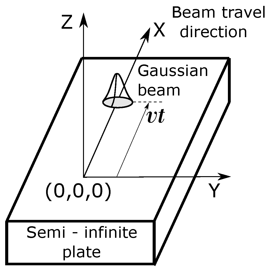
A well-known analytical model developed by Eagar and Tsai [35] that solves for the 3-dimensional temperature field produced by a traveling distributed heat source on a semi-infinite plate is used in the present work. This model has been previously used by several different researchers for evaluating melt pool evolution in laser powder bed fusion (L-PBF) [33] and directed energy deposition (DED) [36] AM processes when extensive evaluation of process parameter space is required. It is a distributed heat source modification of the Rosenthal’s [37,38] solution for the temperature distribution produced by a traveling point heat source. As compared to Rosenthal’s solution, Eagar–Tsai’s model provides a significant improvement in prediction of temperature in the near heat source regions. Figure 2 explains the coordinate system used in the model. The heat source is traveling with a uniform speed of v in the X-direction, and is assumed to be a 2D surface Gaussian:
Here, is the power distribution per unit area on the X–Y plane of the specimen produced by the Gaussian beam of peak power P with a distribution parameter . According to Eagar–Tsai’s model, the temperature , at a particular location and time t, with the initial temperature of the substrate being , is denoted as
Here, is the absorptivity of the laser beam, is the thermal diffusivity, is the density, and c is the specific heat capacity of the material of the specimen. The primary assumptions of the model include the following.
- Convective and radiative heat transfer from the substrate to the environment are ignored. As the process deals with metals which are good conductors, heat transfer through radiation is negligible [39] as compared to that due to conduction.
- The temperature dependence of the thermo-physical properties is not taken into account.
- The substrate is semi-infinite, therefore the increase in the surface temperature with time is negligible.
- Phase change of the material is not taken into consideration.
Eagar–Tsai’s model, despite its limitations (e.g., its inability to model keyholing effect [33]), is widely used in literature for parameter space exploration through design of experiments (DoE)-based approaches. Given the wide range of process parameters in metal AM machines (e.g., L-PBF has over 130 parameters that can affect the final part quality [40]), such a DoE approach would require an exponential number of samples in the dimension of the parameter space to fully explore the design space. This makes it prohibitively expensive to explore the design space for building complex parts through experimentation or high-fidelity simulations. Computationally efficient surrogates can reduce the computational burden by a significant amount. Eagar–Tsai’s model, when appropriately calibrated, provides one such alternative as a low-cost simulation model that are extensively used by several researchers in recent times [33,41,42]. This model especially works well for single-track and single-layer AM depositions. Owing to these characteristics, the validation and control experiments outlined in this paper are all single-track and single-layer.
2.2. Experimental Validation of the Simulation Model
Eagar–Tsai presented experimental validation of their model with a range of process parameters in welding carbon steel plates [35]. Other researchers validated this model for a range of different materials such as nickel- [43], iron- [33], and titanium-based [44] alloys among others to obtain satisfactory accuracy with the experimental data across a range of AM processes, e.g., L-PBF and DED [45], in recent times. However, most of the experimental validation of this model, so far, has been performed under steady state conditions. Being a transient model, Eagar–Tsai’s formulation can potentially be used to simulate the melt pool dimensions as a function of time as well. In this section, both steady and unsteady state validation of the Eagar–Tsai’s formulation are presented.
2.2.1. Steady-State Experimental Validation
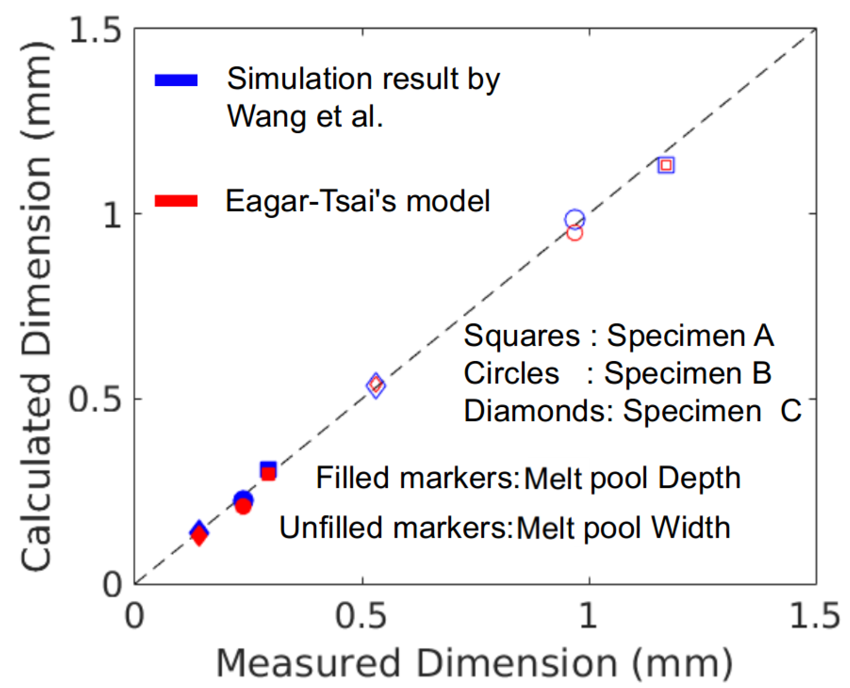
For the steady-state model validation, the melt pool dimensions calculated by Eagar–Tsai’s model are compared with those obtained using finite-element simulations and experiments for a popular nickel-based superalloy CMSX-4 reported by Wang et.al [36]. This alloy was processed by several different researchers using L-PBF [46,47], electron beam powder bed fusion (E-PBF) [48], and DED [49], and therefore a considerable amount of experimental data is available in the open literature. The thermo-physical properties of CMSX-4 chosen in this work are those reported by Gäumann et al. [50]: k = 22 W/(m·K), = 8700 kg/m3, c = 690 J/(kg·K), and the liquidus temperature = 1660 K. Three surface melting experiments were reported by Wang et al. under different processing parameters, as enlisted in Table 1. A CO2 laser beam with radius W was used in their work.
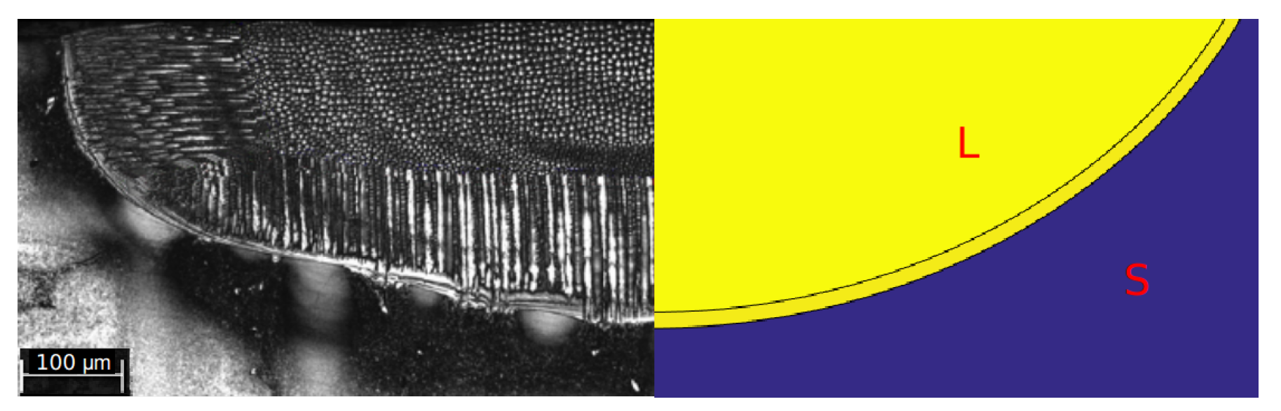
Figure 3 shows the comparison between the current work with those obtained experimentally and using finite element simulations by Wang et al. [36] showing excellent agreement. Figure 4 shows a transverse cross section ( plane, with ) of the analytically calculated melt pool geometry juxtaposed on the fusion zone produced by the process parameters in the CMSX-4 Specimen A, as reported by Wang et al. [36]. Similar agreements are also observed for the other two specimens (i.e., B and C), as evident from the results reported in Figure 3. Cross-sectional images for specimens B and C are omitted for brevity.
2.2.2. Transient Experimental Validation
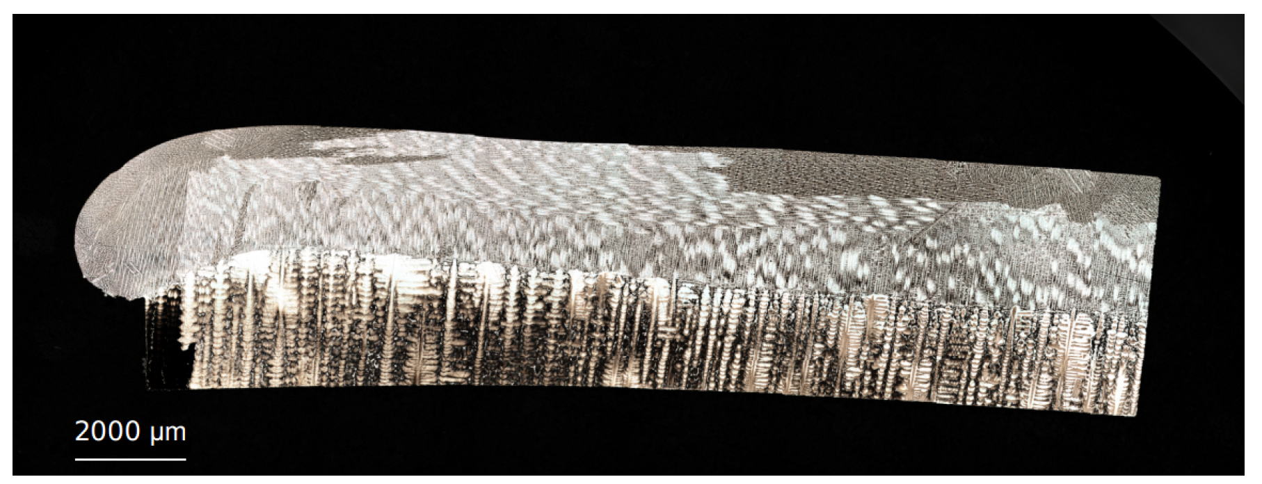
After obtaining excellent agreement with the steady-state results, the analytical model is further validated using transient melt pool results available in the open literature [51]. Figure 5 shows the longitudinal cross section of an L-PBF-processed CMSX-4 specimen. This specimen is fabricated by consolidating a powder layer thickness of 1.4 mm on a CMSX-4 substrate having dimensions of 35.56 mm (length) × 6.86 mm (width) × 2.54 mm (thickness). The process parameters reported are 750 W laser power, 12.7 m raster scan spacing, and 600 mm/s raster scan speed. The raster scanning speed () is related to the linear velocity (v) of the laser in the X direction by .
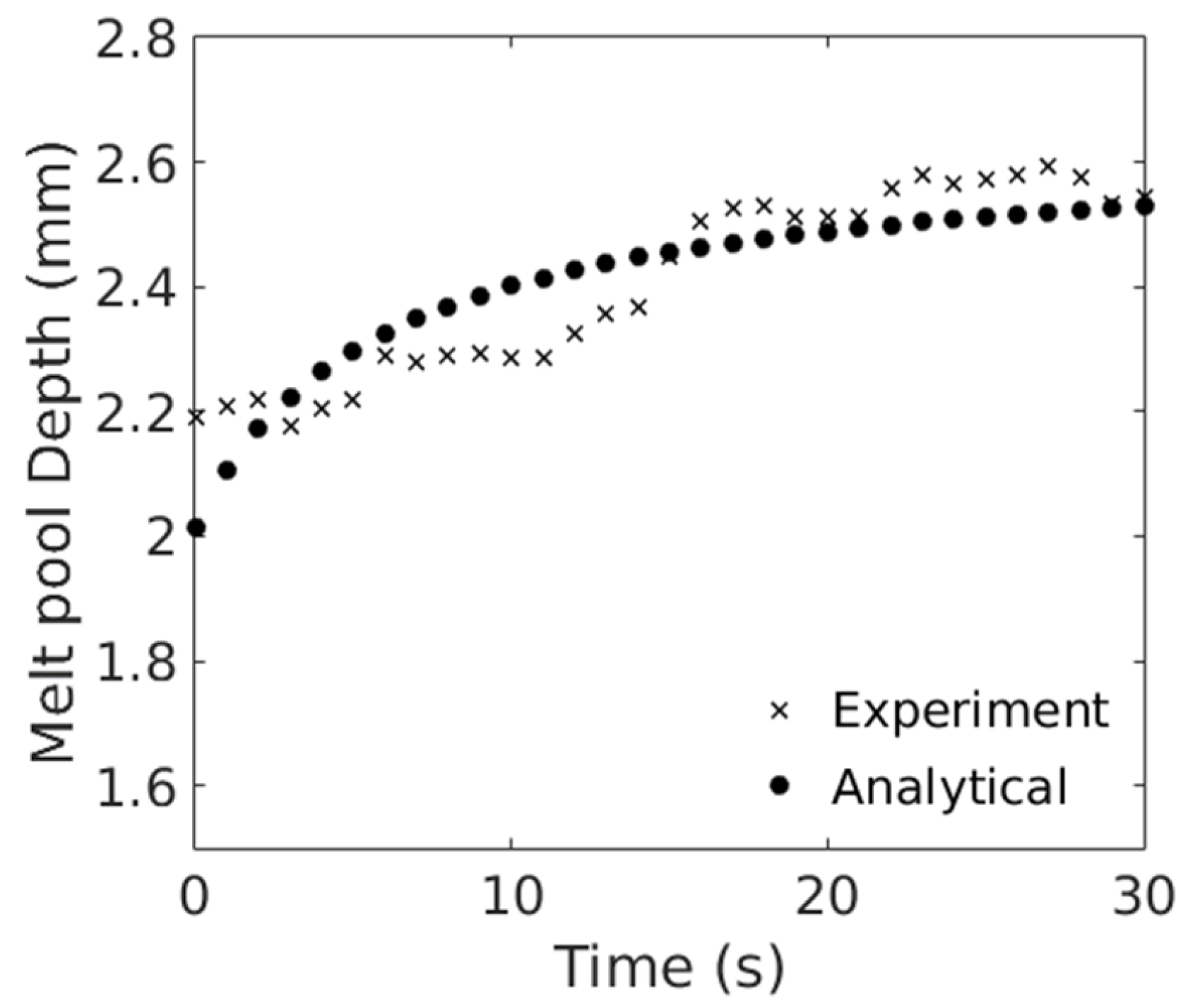
Figure 6 shows the comparison between the analytically calculated and experimentally observed melt pool depth for the CMSX-4 specimen as illustrated in Figure 5. The maximum absolute relative error between the experimental and analytical melt pool depths is ~8% at the start of the scan period, with the mean absolute error during the 30 s period being 2.71%. The results also show the transient nature of the melt pool, with the depth continuously increasing as a function of time with a fixed set of process parameters.
2.3. Hybrid Model
The validation results show that Eagar–Tsai’s model can provide excellent low-cost estimates of melt pool dimensions for single-track and single-layer AM depositions. The goal of this work is to obtain model-based estimates of the required temporal variations in process parameters for achieving target melt pool dimensions during the build process. In order to achieve this, an optimization problem that finds process parameters as a function of time is solved with an objective of minimizing the deviation from the desired melt pool dimensions. As the true functional form that relates the process parameters to the melt pool dimensions is unknown, the information regarding gradients is not readily accessible, therefore the optimization problem is in a black-box setting. Several such black-box optimization techniques are well-studied by different researchers [52], e.g., stochastic process-based approaches (kriging methods) [53], evolutionary algorithms [54], trust-region based algorithms [55], and random search [56]. These approaches typically involve iterative sampling of the objective function in the search space. Such sampling often proves to be prohibitively expensive, particularly in high dimensions, when the involved process model is computationally very expensive.
To address this challenge, in the present work, an application of gradient-free optimization under budget limitations is implemented by solving the melt pool geometry control problem using BO that employs computationally inexpensive GP surrogate models learnt via sparse sampling of the space of process parameters (e.g., P and v). The details of the mathematical formulations of GP and BO can be found in Appendix A. Although all optimization demonstrations in this paper involve the Eagar–Tsai’s model as the process model, it can very well be replaced by any other process models of users’ choice, without any fundamental change in the optimization algorithm.
3. Results and Discussion
This section presents the results and discusses the significant findings therefrom.
3.1. Prediction of Melt Pool Dimensions Using GP
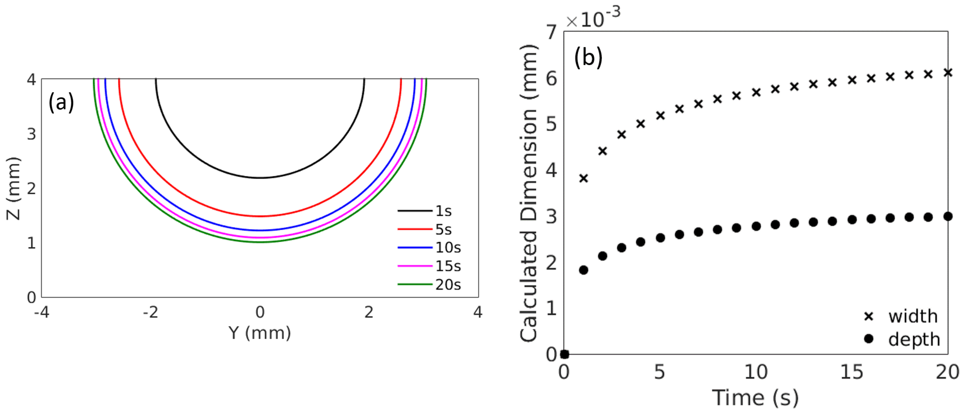
The melt pool dimensions in the L-PBF AM process continuously increase due to progressive heating of the specimen caused by the layer-wise fabrication as evinced by simulation results [57] as well as experimental observation [47]. Figure 7 shows the variation in melt pool dimensions as a function of time for a CMSX-4 specimen fabricated using a laser power of 900 W and linear scan velocity of 0.25 mm/s. The melt pool depth increases from 1.814 mm at t = 1 s to 3 mm at t = 20 s, while the melt pool width increases from 3.82 mm to 6.11 mm. The percentage increase in melt pool depth is ~65%, and the increase in width is ~59%. The melt pool reaches a steady state at ~20 s. If the melt pool dimensions need to be maintained at desired values, the process parameters should be adjusted during this transience period. However, performing simulations for a range of process parameters over the entire deposition process is computationally expensive when coupled with an optimization framework.
In applications where data is scarce, particularly when each simulation can be potentially computationally expensive, it is often infeasible to have a large number of training points. Moreover, inherent uncertainties in the physical process and the simulation models (e.g., uncertainties in the thermophysical properties of the material) mandate the need of uncertainty quantification with the predictions [33,58]. Surrogates, like GPs, can be very useful in such cases in order to have probabilistic estimates of the quantity of interest with limited datasets, whereby the posterior mean and variance can not only be informative for prediction at unknown input locations, but the information can also be used for budget-constrained optimization, as described in the following subsection. A surrogate modeling and optimization technique as discussed in Appendix A is adopted in this work to find the model-based estimates of the process parameters required for controlling the melt pool dimensions.
In order to build the surrogate using GPs, two-hundred (200) Latin hypercube sampling (LHS) simulations are performed to obtain the values of melt pool depth and width at each time instant for combinations of P and v in the range of 300 to 1200 W and 0.5 to 2.5 mm/s, respectively. This parameter range is chosen to avoid any keyhole mode of melt pool formation in CMSX-4 where the Eagar–Tsai’s model shows limited accuracy [59,60]. The cross section of melt pools created in conduction mode is generally semicircular, as predicted by Eagar and Tsai’s conduction mode model [35]. LHS is selected as this is one of the most commonly used statistical methods for DoE. It allows for a good spread of the initial DoE over the design region with limited iterations due to its high sampling efficiency [61]. For every time instant under consideration, each DoE point comprises a combination of process parameters and its corresponding melt pool depth and width values.
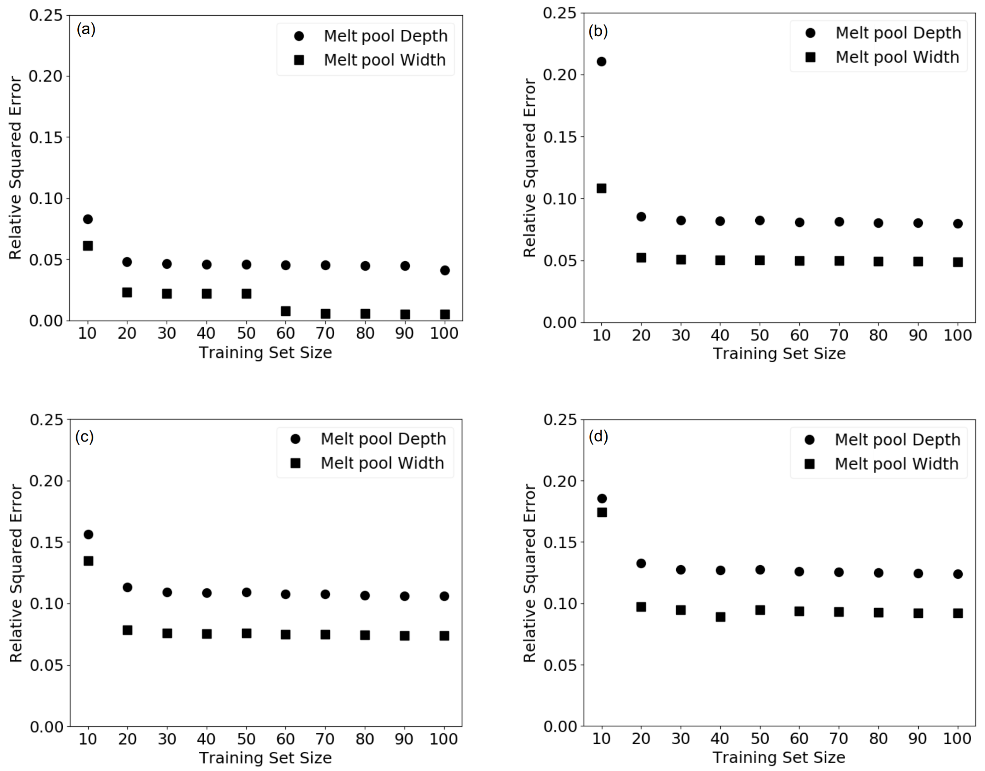
The effect of training data size on the regression performance of the GP surrogate in predicting melt pool depth and width is of critical interest. Out of the 200 initial LHS points, a test set of randomly selected 100 points is set aside for testing the regression performance of the GP models. Different GPs are trained at different time instants with randomly selected samples from the training set. The training data size is varied from 10 to 100, in steps of 10 samples. Ten random selections of the training data is chosen for each training size, in order to find the average behavior of the regression performance for each training size. The prediction performances are tested on the set aside 100 samples for each trained GP model.
The metric for gauging the prediction performance is chosen as the Relative Squared Error (RSE) , where is the prediction and is the true value (i.e., ground truth as obtained by the Eagar–Tsai’s model). A lower RSE suggests that the most likely prediction (mean of the predicted posterior Gaussian distribution) of the depth/width in the test set matches closely with the true value. Figure 8 shows that the RSE is quite low for all the time steps, while there is a slight increase in RSE from 2 s to 20 s for both depth and width. RSEs for the melt pool depth and width prediction show a sharp drop from training size of 10 to 20 samples, after which the RSE saturates for almost all the higher training sizes. This indicates that a training size of at least 20 LHS DoE points is in general sufficient for a satisfactory prediction of the melt pool depth and width in the selected process parameter space. This provides an estimate of the number initial DoE points required for learning the surrogate model for the subsequent BO steps at each time instant.
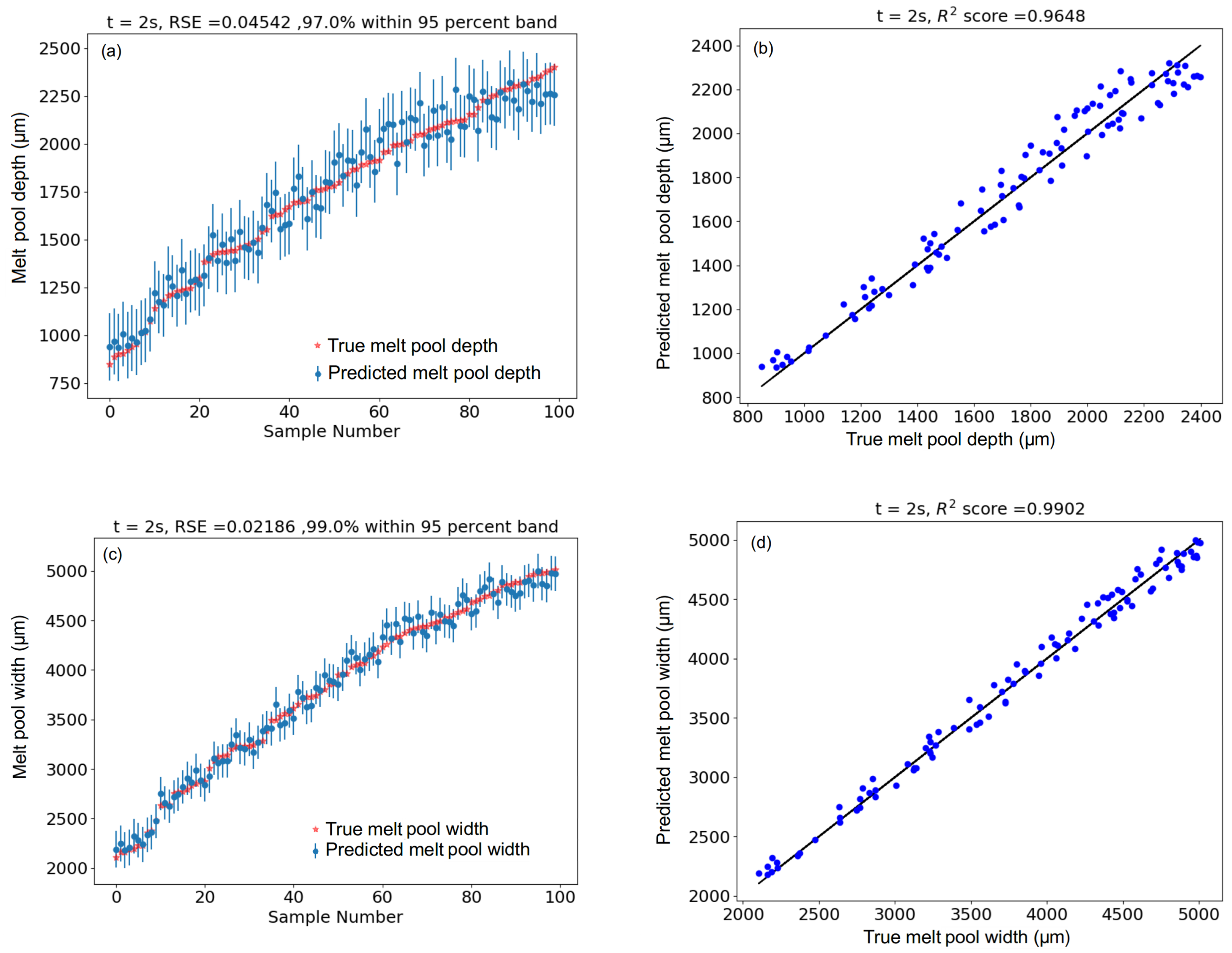
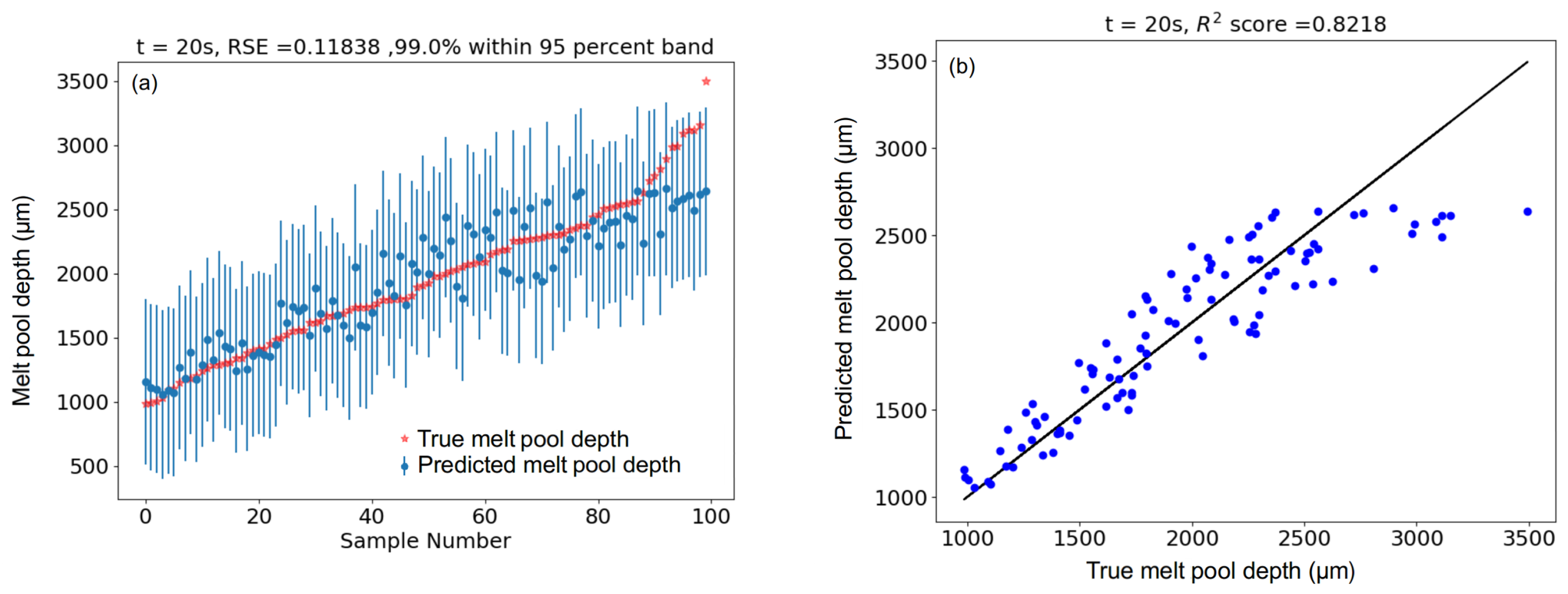
Figure 9 shows the regression performance (on the test dataset of 100 samples) in predicting the melt pool depth and width at 2 s with a training set size of 20. Sample numbers in Figure 9a,c refer to the test samples, which are different combinations. The test samples are arranged in an ascending order of their true depth values. The -band coverage percentage is the proportion of test points for which the true amplitude lies within ±2 of the predicted mean, which corresponds to the 95% confidence interval, as the output distribution is a Gaussian. The parity plots in Figure 9b,d show the comparison of the predicted means with the true values. The high (coefficient of determination) scores for the depth (0.96) and width (0.99) predictions at 2 s indicate high reliability of the GP model in predicting the melt pool dimensions. Similar results are shown in Figure 10 for the melt pool depth and width predictions at 20 s, with a training set size of 20 samples. The score decreases to 0.82 for depth prediction and 0.88 for width prediction, which is also explained by the higher RSE in prediction at 20 s (Figure 8). The variability in the predicted values from the true values is explained by the wider band at the test locations. The lower score at 20 s as compared to 2 s can be attributed to the higher variability in the steady state values of depth and width as compared to the initial stages as a function of the process parameters. From the perspective of applicability of the surrogate predictions, GPs provide the end user with not only a computationally inexpensive way of predicting the melt pool dimensions at different operating conditions for which experiments and simulations are not performed, but also with an estimate of uncertainty quantification (UQ) for predictions from the variance associated at the query points.
3.2. Optimization of Process Parameters for Melt Pool Dimension Control: Objective Function
As discussed in Section 1 and Section 2, appropriate control of the process parameters, e.g., P and v are required for maintaining desired melt pool dimensions during the deposition process. The goal of controlling the melt pool dimensions is formulated as an objective function that needs to be maximized in the setting of BO, as described in Appendix A.3. In order to pose the melt pool control problem in an optimization setting, an appropriately defined objective function (J) is to be maximized at every discrete time instant of control,
where d and W denote the depth and width, respectively, at a particular time instant, whereas and represent the desired depth and width, respectively, during the deposition process. P indicates the power at time instants of control, whereas and denote the maximum and minimum values of the range of laser power in the space of process parameters. Therefore, denotes the normalized power input at a particular time instant, and incorporating it into the objective functional serves as a penalty term for high power values. This is introduced since it is desired to achieve the controlled process along with avoiding processing conditions involving very high levels of power.
, , and in Equation (3) denote the relative weights of the components of the objective function that controls the depth, width, and power, respectively. By varying the relative values of , , and , it is possible to preferentially weigh the objective function to meet the requirements. Formulating the objective functional J is a key step in the optimization process, and the optimization routine should be designed in such a way that undesirable process parameters result in low values of objectives. This formulation conforms to the mathematical characteristics of the Matérn covariance function [15] used in this work, which assumes local smoothness of the inputs, so that input process parameters that are close together in the space are expected to have similar objective values. As undesirable parameter combinations have low objectives, points in the close vicinity of them will have low acquisition potential (see Appendix A) during the optimization steps, and therefore will have lower priority for the incumbent selection.
3.3. Optimization Routine
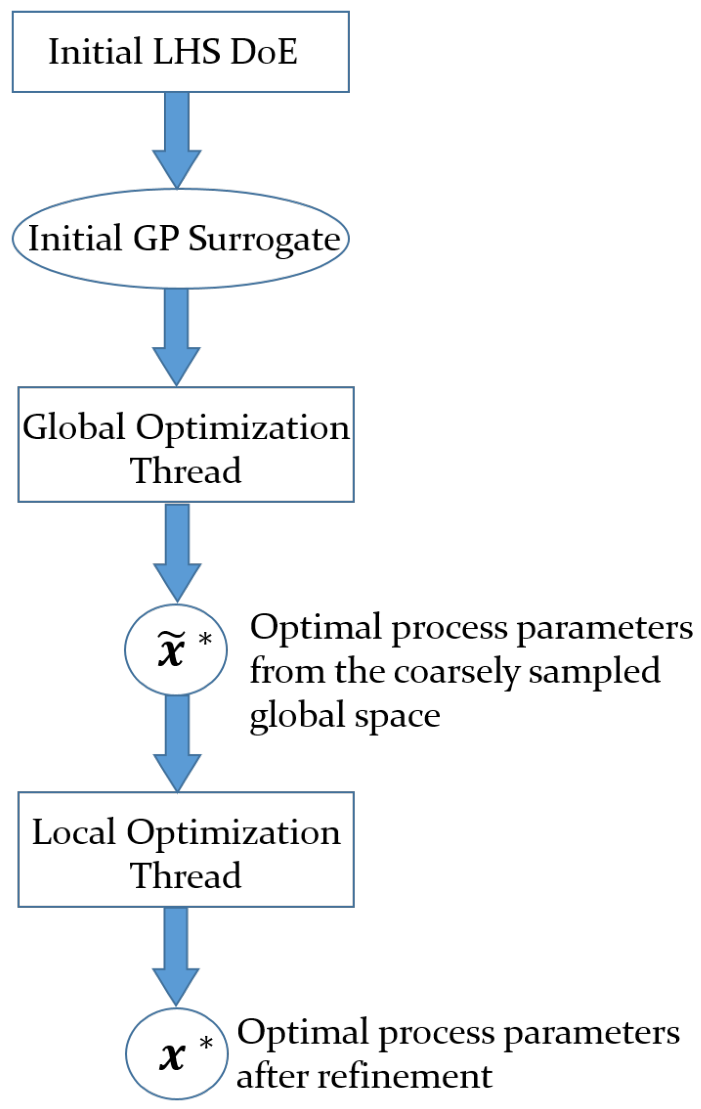
A sequential global–local optimization thread [62] is employed in this work for the selection of process parameters for controlling the melt pool geometry. The terms “global” and “local” correspond to the search spaces with respect to which BO is performed. In the global optimization thread, a potential optimal process parameter combination is selected, around which a refinement is made during the local optimization thread for the final selection of the optimal process parameter combination. The outline of the process is described in the flowchart as depicted in Figure 11. Details of the optimization algorithm can be found in Appendix B. Entities capped with “tilde” (∼) correspond to parameters of the local optimization thread.
The control problem is designed to maintain the melt pool depth at 2.5 mm and width at 5.0 mm. The initial global GPs are learnt with 20 LHS points in the space, with W and mm/s. The ranges of the process parameters and the controlled geometrical parameters chosen in this problem are often dictated by the experimental requirements and constraints, and can be modified as needed. The optimization problem over the entire duration of the L-PBF process can be considered as a sequence of optimization problems performed at some discrete intervals of time, which motivates the choice of learning separate surrogates for each discrete time instant for which the melt pool needs to be controlled.
With the initial trained GP from 20 LHS samples for each time instant, low-cost surrogate predictions are made over the large global search space , consisting of 2000 uniformly chosen points. This methodology forms the key to the surrogate-based optimization processes: predictions are made over an extensive search space by employing a low-cost surrogate by avoiding functional evaluations (physics-based simulations in this case) at the search points. Based on the mean–variance trade-off of the GP’s posterior predictive distribution, the acquisition function (See Appendix A) guides the search iteratively to subsequent optimization points until the computational budget is depleted. optimization steps are chosen for the global thread, after which the optimal process parameter combination with the highest objective value is selected.
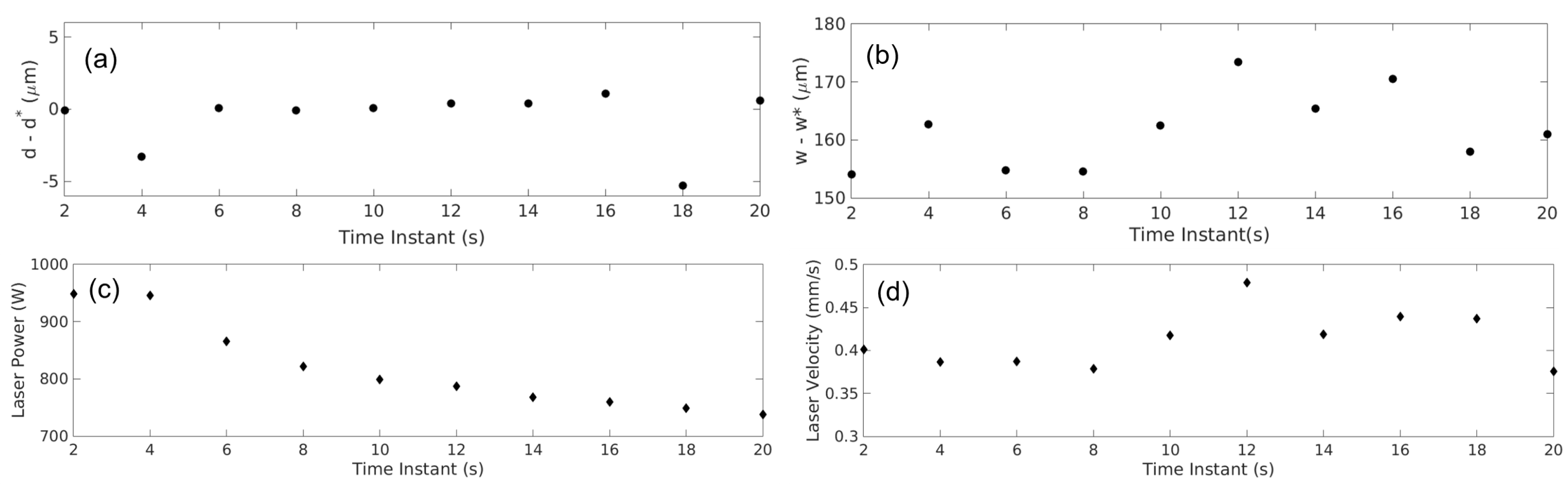
For all the time instants of control, it was possible to obtain optimal process parameters within the global thread that can yield the melt pool depth and width close to the desired values. However, for finer adjustments in P and v values in order to achieve the micron-level control in the melt pool geometry, the local optimization thread is executed. Here, the local search space is built around , the optimum with the highest objective value from the global thread, in the following way; P is varied within W and v within mm/s of the corresponding values in . 20 LHS points are chosen within the limits of , the optimization routine is performed within this local search space for steps. This yields the refinement of the process parameter values that result in melt pool dimensions very close to the ones desired. The number of optimization iterations in both the local and global threads (i.e., and ) are kept as design parameters in this paper, which are expected to be driven by computational budget for practical applications. The scaling factors for the objective function components are chosen as , , and , which are based on the greater relative importance of maintaining the depth as close to as possible during the build process, so that a uniform deposit is maintained.
Figure 12 shows the performance of the surrogate based optimization method. Figure 12a,b shows the variation of the controlled melt pool depth and width from the desired and values as a function of time. It is seen that the maximum variation in the meltpool depth is 1.1 m which is 0.04% of the desired depth, while that for width is 173 m, which is 3.46% of the desired width. The process parameters change from P = 948.07 W, v = 0.40 mm/s at t = 2 s to P = 737.81 W, v = 0.37 mm/s at t = 20 s (Figure 12c,d). It is to be noted that penalization of P in the objective function allows us to have a smoothly variation of P over 20 s with lower P values, which changes by ~22% of the starting value at t = 2 s. The maximum change in v is ~27%. It is possible to have process parameters with higher P values (and higher v values) that control the melt pool, but those conditions are avoided by P penalization in the objective function. Similar formulation of the objective function can be pursued by v penalization, if smother v transition is desired.
3.4. Validation with Experimental Results of Melt Pool Depth Control
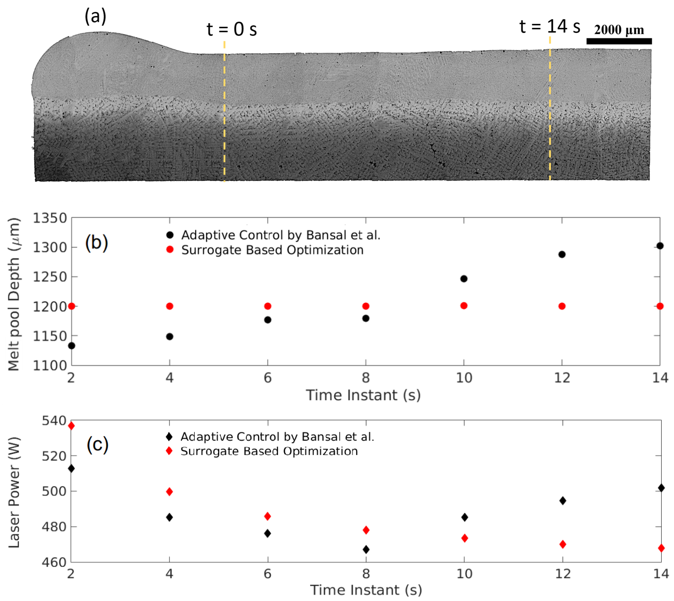
The model-based control strategy is validated with experimental results reported in the open literature [63]. Figure 13a shows the longitudinal cross section of an L-PBF processed René 80 specimen fabricated using a powder layer thickness of 1.4 mm on a substrate of dimensions 35.56 mm × 6.86 mm × 2.54 mm. The experiment was carried out with the raster scanning speed of 450 mm/s and scan spacing of 25.4 m. In reality, experiments are extremely challenging to perform with melt pool depth as a controlled variable as there exists no easy way of measuring the melt pool depth in situ. During the conduction mode, the surface temperature control of melt pools was found to correlate well with the melt pool depth experimentally by Bansal et al. [63]. The observation was also made by Raghavan et al. in E-PBF of Inconel 718 [64]. The mean value of the melt pool depth during the control period is around 1200 m from experiments. Accordingly, is set at 1200 m for the surrogate-based optimization routine involving only P as outlined in the experiments.
The melt pool simulation is performed by employing the Eagar–Tsai’s model, with the thermo-physical properties of solid René 80: W/(m·K), = 7604 kg/m3, J/(kg·K), and the liquidus temperature = 1607 K obtained using the software JMatPro [65], with the alloy composition of René 80 provided by the vacuum alloy product catalog of Cannon Muskegon [66]. The objective function involves two components in this case:
with and .
Figure 13 shows that the predicted melt pool depth with the surrogate assisted control scheme remains very close to the desired . A variation of ∼200 m is observed in the experimental results, whereby the melt pool depth shows a slightly increasing trend towards the end of the control process, reflected by the slight increase in power input from 10 s till 14 s. The trend of the surrogate predicted controlled power input matches closely with the experimental results till 8 s, which is explained by the fact that for a constant laser speed, the power input should decrease as a function of time in order to maintain a constant melt pool depth as the specimen gains thermal energy continuously. Nonetheless, the validation results indicate the efficacy of the surrogate-based optimization routine in predicting process parameters as a function of time for achieving melt pool dimension control during the deposition process.
4. Summary and Conclusions
This paper develops a novel hybrid methodology for control of melt pool geometry in AM in the framework of ML-assisted modeling and optimization. The continuous changes in the melt pool geometry are predicted by a low-cost GP surrogate developed using an experimentally validated analytical 3D model. The uncertainties in the predictions for the melt pool geometry are quantified using GPs. Reliable estimates of the optimal process parameter evolution are obtained through active learning via BO by devising appropriate objective functions that quantify the control requirements. The methodology provides an estimation of process parameter variation during the AM deposition process in order to maintain a desired melt pool geometry under continuously varying thermal conditions.
Being data-driven, the reliability of the optimized process parameters obtained from the algorithm is based on the accuracy of the underlying physical model in predicting the melt pool geometry in the range of process parameters considered. However, with a high-fidelity model, the computational cost involved in the optimization process can be significantly high. For example, the cost of running a Netfabb [67] DED model for a single-track and single-layer process on a CMSX-4 specimen as described in this paper is ∼10 times as expensive as Eagar–Tsai’s model at t = 2 s, and ∼150 times at t = 10 s. Although such high-cost simulation is prohibitive in practical applications, in the future, the methodology will be enhanced by using information from different fidelities [68] of AM computational models to develop a multifidelity modeling and optimization framework for prediction and control of melt pool geometries. For example, a Netfabb model can be combined with inexpensive observations from Eagar–Tsai’s model to develop a two-fidelity GP that can be used for melt pool geometry prediction and optimization with an expected reduction in computational cost. Additional investigations are also planned as summarized below.
- Usage of process parameters (other than P and v) such as scan spacing (i.e., hatch spacing), scan pattern (i.e., hatch pattern), build plate temperature, and powder layer thickness (for powder bed AM) and powder feed rate (for directed energy AM) as control inputs.
- Incorporation of design constraints in the surrogate assisted modeling framework, e.g., tackling harder problems whereby a melt pool geometry needs to be controlled, along with the final microstructure such as columnar grains in CMSX-4.
- Development of heterogeneous design spaces in formulating multifidelity modeling framework, which can be useful in catering to optimization problems where the varied levels of fidelities have different input spaces. As an example, a HF L-PBF process model can have several process parameters, such as powder distribution properties, hatch spacing, scan strategy, etc., apart from P and v of the laser (which are the only process parameters for a LF model like the Eagr-Tsai’s model), which can potentially affect the build characteristics. Optimization in such a framework can be possible via heterogeneous transfer learning [69] to learn from a common subspace of the inputs.
- Integration of the surrogate modeling framework developed in this work with microstructure prediction framework using an open source SPPARKS code [70] to optimize the process parameters for obtaining a desired microstructure.
- Implementation of the surrogate modeling framework for checking its efficacy towards mitigating unintended melt pool behavior such as keyholing effect. However, in such a case, the computational model needs to be a high fidelity one capable of predicting such a behavior.
It is envisioned that the newly developed framework can be implemented in developing feedback strategies for melt pool control during AM processes with shorter response time due to improved prediction capability [71].
Author Contributions
Conceptualization, S.M. and A.B.; methodology, S.M.; software, S.M. and D.G.; validation, S.M., A.B. and D.G.; formal analysis, S.M.; investigation, S.M. and A.B.; resources, A.B. and A.R.; writing–original draft preparation, S.M. and A.B.; writing–review and editing, A.B., S.M. and A.R.; visualization, S.M.; supervision, A.B. and A.R.; funding acquisition, A.R. and A.B. All authors have read and agreed to the published version of the manuscript.
Funding
This research was funded in part by U.S. Air Force Office of Scientific Research (AFOSR) under Grant # FA9550-15-1-0400 in the area of dynamic data-driven application systems (DDDAS). Any opinions, findings, and conclusions in this paper are those of the authors and do not necessarily reflect the views of the sponsoring agencies.
Conflicts of Interest
The authors declare no conflict of interest.
Appendix A. Mathematical Background
This section provides the mathematical background for machine learning (ML)-assisted modeling and optimization of additive manufacturing (AM) processes. While the details are available in standard literature (see, e.g., in [72,73]), the following three subsections succinctly present the core concepts of ML for completeness of the paper.
Appendix A.1. Surrogate Modeling: Gaussian Processes
This subsection provides a brief overview of the surrogate modeling technique using Gaussian Processes (GPs), which is the foundation of the Bayesian Optimization (BO) framework used in this work for control of melt pool geometry. Salient properties of GPs modeling are delineated below.
- GPs belong to a class of stochastic processes based on the assumption of a multivariate jointly Gaussian distribution for any finite collection of random variables.
- GPs are nonparametric models that do not assume a predefined functional relationship between the inputs and outputs (unlike polynomial regression models [73], for example).
- GPs are flexible for modeling nonlinear functions. As the underlying concept is fully Bayesian, the predictions are made via a posterior probability distribution, which is a normal distribution in case of GPs, completely specified by its mean and covariance.
Remark A1.
The main advantage in having a probabilistic prediction method is that it naturally provides a measure of uncertainty quantification (UQ) associated with these predictions through the variance of the distribution. Moreover, having a probabilistic estimate instead of a fixed estimate provides the end user with a confidence level of the predictions.
For a finite subcollection of the random input , the corresponding objective values
are assumed to have a multivariate jointly Gaussian distribution:
where the mean and the covariance , and indicates the expectation of a random variable.
Let , be the training set that are available for model formulation. For a noisy regression model, it is assumed that
where the additive noise are independent and identically distributed (iid) zero-mean Gaussian random variables, i.e., . By incorporating the noise term, the joint distribution of the observed values and the functional values at the test locations are
where is the test set in which is online observed data and is the unknown variables to be estimated. Therefore, by the property of multivariate normal distributions, the conditional distribution of the function values at the test location is Gaussian [72]. In particular,
where
Thus, the algorithm predicts the mean and covariance for the posterior distribution that models the output at every test data point.
Appendix A.2. Kernel Function
The choice of the covariance function is one of the most critical aspects of the model selection process in GP-based surrogates. It is assumed that the objective function is locally smooth and that the GP priors belong to the class of automatic relevance determination (ARD) Matérn covariance functions [15]. The ARD formulation facilitates learning a length-scale for each input dimension to deal with directional anisotropies in the data set. The Matérn class of covariance functions has a shape parameter that can be tuned in order to control the smoothness of the correlation function in the input space. In this work, a Matérn shape parameter of 5/2 is used, which results in the form , where . The hyperparameters in the kernel are , where D is the dimensionality of the data set, and and are the scaling coefficient and the characteristic length-scales, respectively.
Instead of squared exponential kernels that are generally best suited for interpolating smooth functional relationships, Matérn kernels are chosen here because length-scales associated with the latter are less prone to be affected by the presence of non-smooth regions in the data set, which might yield poor extrapolation results in the smoother regions [74].
Appendix A.3. Bayesian Optimization
In this work, the term optimization is used to denote maximization of a target function, without any loss of generality. A minimization problem can be posed similarly by taking the negative of the target function. Therefore, in order to optimize an objective function f, the following solution is sought.
If the functional form of f is unknown, it may not be possible to have gradient-based optimization for solving the problem; in that case, gradient-free or black-box optimization might be suitable. BO is one such black-box optimization technique [31] that leverages the predictions through a surrogate model for sequential active learning (AL) to find the global optima of the objective function. The AL strategies are aimed at finding a trade-off between exploration and exploitation in possibly noisy settings [52,75,76], which facilitates a balance between global search and local optimization through acquisition functions. Usage of GPs in the surrogate modeling framework for BO often leads to closed-form analytical expressions for acquisition functions, which are inexpensive to compute.
In the above formulation, the acquisition functions are designed in the following way. The potential of performance improvement is driven by the predicted mean function (which is in the category of exploitation), whereas the uncertainty prediction is manifested by regions of high variance (which is in the category of exploration). A trade-off between these two requirements is achieved by the acquisition functions iteratively, as a sequential optimization process.
Figure A1.
Sequence of Bayesian Optimization iterations for maximizing . (a) Iteration : Prediction based on initial DOE of 4 points. (b) Iteration . (c) Iteration . (d) Iteration . Filled blue circles indicate initial DOE. Filled red circles denote points selected in optimization iterations.
Figure A1.
Sequence of Bayesian Optimization iterations for maximizing . (a) Iteration : Prediction based on initial DOE of 4 points. (b) Iteration . (c) Iteration . (d) Iteration . Filled blue circles indicate initial DOE. Filled red circles denote points selected in optimization iterations.

One commonly used acquisition function in Bayesian optimization is Expected Improvement (EI), which is employed in this work. According to the formulation of Mockus et al. [77] and Jones et al. [52], the EI acquisition function can be written as
where
and is the input corresponding to the maximum functional value sampled until iteration k; the parameter controls the trade-off between exploration and exploitation [31]; and are the mean and variance, respectively, predicted by the GPs for the an input point ; and and are the probability distribution function (PDF) and cumulative distribution function (CDF) of the standard normal distribution, respectively.
If the objective function is noise corrupted, instead of using the best observation, the point with the highest expected value is defined as the incumbent, i.e., replaced by , which is defined as
The optimization algorithm proceeds sequentially by sampling at every step of the iteration process to add on to the dataset, after which the GP model is retrained with the new data set to predict the acquisition potential for the next iterative step. This process continues until an optimum is reached, or the computational budget is extinguished. As the acquisition potential is predicted over the entire search space by the surrogate, BO can achieve fast predictions without a lot of function calls in the search space (i.e., without having to run the simulations to obtain the objectives at all the search locations), which, otherwise, might be computationally infeasible when the search space is high-dimensional and the simulations are expensive.
Figure A1 demonstrates the optimization process through a simple problem of maximizing a black-box function in the input space of (denoted by solid blue line). The process is started with an initial design of experiments (DoE) of 4 points (filled blue circles) chosen in the search domain by Latin hypercube sampling (LHS) [61], which allows the initial selection of points to be well-spread in the search space. Figure A1a shows the GP prediction in the initial stage, which is characterized by the mean function (red dotted line), and the variance associated with the prediction (denoted by the orange band). The variance is high globally at the initial stage, because only four points are sampled on the true function. The maximizer of the acquisition function shows the location to sample for the next point at every iteration (filled red circles). Figure A1b shows that the predicted mean of the function in Figure A1a drives the selection of the first optimization point. It is interesting to note that in Figure A1c, although the true maximizer of is already sampled, points towards a region where the variance is high. This is because of the exploration-exploitation trade-off which allows the algorithm to explore the search space instead of greedily searching for the optimum, a property that helps the algorithm avoid being stuck at a local optima. Eventually after seven optimization iterations, the routine converges at the true optima, as shown in Figure A1d. Moreover, the mean function predicted at the last stage is very close to the true function, and the uncertainty band also reduces globally, which indicates that the algorithm not only finds the maximizer of the function, but in doing so it also learns a pretty accurate surrogate model of the function, which can now be used as a low-cost approximation of the true function.
Appendix B. Optimization Algorithm
Algorithm A1 shows the surrogate-based optimization routine that is employed in this paper for solving the melt pool geometry control problem, which is elucidated in Section 3.3. The global thread picks up an optimal point , which is refined in the local thread to give , as the final optimal point chosen by the algorithm.
| Algorithm A1 Optimization Routine |
| Global Thread |
| Require: Start with surrogate GP for the objective functional J with LHS initialization |
for optimization steps do
|
| end for |
|
| Local Thread |
| Require: Start with surrogate local GP for the objective functional J with LHS initializations |
for optimization steps do
|
| end for |
| - Select |
References
- DebRoy, T.; Wei, H.; Zuback, J.; Mukherjee, T.; Elmer, J.; Milewski, J.; Beese, A.; Wilson-Heid, A.; De, A.; Zhang, W. Additive manufacturing of metallic components–Process, structure and properties. Prog. Mater. Sci. 2018, 92, 112–224. [Google Scholar] [CrossRef]
- Chua, C.K.; Wong, C.H.; Yeong, W.Y. Chapter Seven-Process Control and Modeling. In Standards, Quality Control, and Measurement Sciences in 3D Printing and Additive Manufacturing; Chua, C.K., Wong, C.H., Yeong, W.Y., Eds.; Academic Press: Cambridge, MA, USA, 2017; pp. 159–179. [Google Scholar] [CrossRef]
- Basak, A.; Das, S. Epitaxy and Microstructure Evolution in Metal Additive Manufacturing. Annu. Rev. Mater. Res. 2016, 46, 125–149. [Google Scholar] [CrossRef]
- Dinda, G.; Dasgupta, A.; Mazumder, J. Laser aided direct metal deposition of Inconel 625 superalloy: Microstructural evolution and thermal stability. Mater. Sci. Eng. A 2009, 509, 98–104. [Google Scholar] [CrossRef]
- Wei, H.L.; Mukherjee, T.; DebRoy, T. Grain Growth Modeling for Additive Manufacturing of Nickel Based Superalloys. In Proceedings of the 6th International Conference on Recrystallization and Grain Growth (ReX&GG 2016); Springer International Publishing: Cham, Switzerland, 2016; pp. 265–269. [Google Scholar]
- Liu, P.; Wang, Z.; Xiao, Y.; Horstemeyer, M.F.; Cui, X.; Chen, L. Insight into the mechanisms of columnar to equiaxed grain transition during metallic additive manufacturing. Addit. Manuf. 2019, 26, 22–29. [Google Scholar] [CrossRef]
- Wang, L.; Felicelli, S.; Gooroochurn, Y.; Wang, P.; Horstemeyer, M. Optimization of the LENS® process for steady molten pool size. Mater. Sci. Eng. A 2008, 474, 148–156. [Google Scholar] [CrossRef]
- Francois, M.; Sun, A.; King, W.; Henson, N.; Tourret, D.; Bronkhorst, C.; Carlson, N.; Newman, C.; Haut, T.; Bakosi, J.; et al. Modeling of additive manufacturing processes for metals: Challenges and opportunities. Curr. Opin. Solid State Mater. Sci. 2017, 21, 198–206. [Google Scholar] [CrossRef]
- Acharya, R.; Sharon, J.A.; Staroselsky, A. Prediction of microstructure in laser powder bed fusion process. Acta Mater. 2017, 124, 360–371. [Google Scholar] [CrossRef]
- Razvi, S.S.; Feng, S.; Narayanan, A.; Lee, Y.T.T.; Witherell, P. A Review of Machine Learning Applications in Additive Manufacturing. In Proceedings of the 39th Computers and Information in Engineering Conference, Anaheim, CA, USA, 18–21 August 2019; Volume 1. [Google Scholar] [CrossRef]
- Lee, S.; Peng, J.; Shin, D.; Choi, Y.S. Data analytics approach for melt-pool geometries in metal additive manufacturing. Sci. Technol. Adv. Mater. 2019, 20, 972–978. [Google Scholar] [CrossRef] [Green Version]
- Qi, X.; Chen, G.; Li, Y.; Cheng, X.; Li, C. Applying Neural-Network-Based Machine Learning to Additive Manufacturing: Current Applications, Challenges, and Future Perspectives. Engineering 2019, 5, 721–729. [Google Scholar] [CrossRef]
- Gilpin, L.H.; Bau, D.; Yuan, B.Z.; Bajwa, A.; Specter, M.; Kagal, L. Explaining Explanations: An Overview of Interpretability of Machine Learning. In Proceedings of the IEEE 5th International Conference on Data Science and Advanced Analytics (DSAA), Turin, Italy, 1–3 October 2018; pp. 80–89. [Google Scholar] [CrossRef] [Green Version]
- Yoshida, Y.; Miyato, T. Spectral Norm Regularization for Improving the Generalizability of Deep Learning. arXiv 2017, arXiv:1705.10941. [Google Scholar]
- Rasmussen, C.; Williams, C. Gaussian Processes for Machine Learning (Adaptive Computation and Machine Learning); The MIT Press: Cambridge, MA, USA, 2005. [Google Scholar]
- Tapia, G.; Khairallah, S.; Matthews, M.; King, W.; Elwany, A. Gaussian process-based surrogate modeling framework for process planning in laser powder-bed fusion additive manufacturing of 316L stainless steel. Int. J. Adv. Manuf. Technol. 2018, 94, 3591–3603. [Google Scholar] [CrossRef]
- Sacks, J.; Welch, W.; Mitchell, T.; Wynn, H. Design and Analysis of Computer Experiments. Statist. Sci. 1989, 4, 409–423. [Google Scholar] [CrossRef]
- Hevesi, J.; Flint, A.; Istok, J. Precipitation Estimation in Mountainous Terrain Using Multivariate Geostatistics. Part II: Isohyetal Maps. J. Appl. Meteorol. 1992, 31, 677–688. [Google Scholar] [CrossRef] [Green Version]
- Rios, L.; Sahinidis, N. Derivative-free optimization: A review of algorithms and comparison of software implementations. J. Glob. Optim. 2013, 56, 1247–1293. [Google Scholar] [CrossRef] [Green Version]
- Bhosekar, A.; Ierapetritou, M. Advances in surrogate based modeling, feasibility analysis, and optimization: A review. Comput. Chem. Eng. 2018, 108, 250–267. [Google Scholar] [CrossRef]
- Kleijnen, J. Kriging metamodeling in simulation: A review. Eur. J. Oper. Res. 2009, 192, 707–716. [Google Scholar] [CrossRef] [Green Version]
- Ong, Y.; Nair, P.; Keane, A. Evolutionary Optimization of Computationally Expensive Problems via Surrogate Modeling. AIAA J. 2003, 41, 687–696. [Google Scholar] [CrossRef] [Green Version]
- Jin, Y. Surrogate-assisted evolutionary computation: Recent advances and future challenges. Swarm Evol. Comput. 2011, 1, 61–70. [Google Scholar] [CrossRef]
- Ramakrishnan, N.; Bailey-Kellogg, C.; Tadepalli, S.; Pandey, V.N. Gaussian Processes for Active Data Mining of Spatial Aggregates. In Proceedings of the 2005 SIAM International Conference on Data Mining, Newport Beach, CA, USA, 21–23 April 2005; pp. 427–438. [Google Scholar] [CrossRef] [Green Version]
- Perdikaris, P.; Venturi, D.; Royset, J.O.; Karniadakis, G.E. Multi-fidelity modelling via recursive co-kriging and Gaussian Markov random fields. Proc. R. Soc. Lond. A Math. Phys. Eng. Sci. 2015, 471. [Google Scholar] [CrossRef] [Green Version]
- Le Gratiet, L. Multi-Fidelity Gaussian Process Regression for Computer Experiments. Ph.D. Thesis, Université Paris-Diderot, Paris, France, 2013. [Google Scholar]
- Liu, B.; Zhang, Q.; Gielen, G.G.E. A Gaussian Process Surrogate Model Assisted Evolutionary Algorithm for Medium Scale Expensive Optimization Problems. IEEE Trans. Evol. Comput. 2014, 18, 180–192. [Google Scholar] [CrossRef] [Green Version]
- Shan, S.; Wang, G. Survey of modeling and optimization strategies to solve high-dimensional design problems with computationally-expensive black-box functions. Struct. Multidiscip. Optim. 2010, 41, 219–241. [Google Scholar] [CrossRef]
- Yang, Z.; Eddy, D.; Krishnamurty, S.; Grosse, I.; Denno, P.; Witherell, P.; Lopez, F. Dynamic Metamodeling for Predictive Analytics in Advanced Manufacturing. Smart Sustain. Manuf. Syst. 2018, 2, 18–39. [Google Scholar] [CrossRef]
- Kuya, Y.; Takeda, K.; Zhang, X.; Forrester, A.I.J. Multifidelity Surrogate Modeling of Experimental and Computational Aerodynamic Data Sets. AIAA J. 2011, 49, 289–298. [Google Scholar] [CrossRef]
- Brochu, E.; Cora, V.; de Freitas, N. A Tutorial on Bayesian Optimization of Expensive Cost Functions, with Application to Active User Modeling and Hierarchical Reinforcement Learning; Technical Report TR-2009-23; Department of Computer Science, University of British Columbia: Vancouver, BC, Canada, 2010. [Google Scholar]
- Tapia, G.; Elwany, A.; Sang, H. Prediction of porosity in metal-based additive manufacturing using spatial Gaussian process models. Addit. Manuf. 2016, 12, 282–290. [Google Scholar] [CrossRef]
- Seede, R.; Shoukr, D.; Zhang, B.; Whitt, A.; Gibbons, S.; Flater, P.; Elwany, A.; Arroyave, R.; Karaman, I. An ultra-high strength martensitic steel fabricated using selective laser melting additive manufacturing: Densification, microstructure, and mechanical properties. Acta Mater. 2020, 186, 199–214. [Google Scholar] [CrossRef]
- Beuth, J.L.; Fox, J.; Gockel, J.; Montgomery, C.; Yang, R.; Qiao, H.; Soylemez, E.; Reeseewatt, P.; Anvari, A.; Narra, S.P.; et al. Process Mapping for Qualification Across Multiple Direct Metal Additive Manufacturing Processes. In Proceedings of the Solid Freeform Fabrication, Austin, TX, USA, 3–5 August 2013; pp. 655–665. [Google Scholar]
- Eagar, T.; Tsai, N. Temperature fields produced by traveling distributed heat sources. Weld. Res. Suppl. 1983, 62, 346–355. [Google Scholar]
- Wang, G.; Liang, J.; Zhou, Y.; Jin, T.; Sun, X.; Hu, Z. Prediction of Dendrite Orientation and Stray Grain Distribution in Laser Surface-melted Single Crystal Superalloy. J. Mater. Sci. Technol. 2017, 33, 499–506. [Google Scholar] [CrossRef]
- Rosenthal, D. Mathematical Theory of Heat Distribution During Welding and Cutting. Weld. J. 1941, 20, 220s–234s. [Google Scholar]
- Rosenthal, D. The Theory of Moving Sources of Heat and its Applications. Trans. ASME 1946, 68, 849–866. [Google Scholar]
- Foteinopoulos, P.; Papacharalampopoulos, A.; Stavropoulos, P. On thermal modeling of Additive Manufacturing processes. CIRP J. Manuf. Sci. Technol. 2018, 20, 66–83. [Google Scholar] [CrossRef]
- Yadroitsau, I. Selective Laser Melting: Direct Manufacturing of 3D-Objects by Selective Laser Melting of Metal Powders, 2nd ed.; Lambert Academic Publishing: Saarbrücken, Germany, 2009. [Google Scholar]
- Kamath, C.; Fan, Y.J. Regression with small data sets: A case study using code surrogates in additive manufacturing. Knowl. Inf. Syst. 2018, 57, 475–493. [Google Scholar] [CrossRef]
- Rubenchik, A.M.; King, W.E.; Wu, S.S. Scaling laws for the additive manufacturing. J. Mater. Process. Technol. 2018, 257, 234–243. [Google Scholar] [CrossRef]
- Gao, Z.; Ojo, O. Modeling analysis of hybrid laser-arc welding of single-crystal nickel-base superalloys. Acta Mater. 2012, 60, 3153–3167. [Google Scholar] [CrossRef]
- Patel, S.; Vlasea, M. Melting modes in laser powder bed fusion. Materialia 2020, 9, 100591. [Google Scholar] [CrossRef]
- Olleak, A.; Xi, Z. Calibration and Validation Framework for Selective Laser Melting Process Based on Multi-Fidelity Models and Limited Experiment Data. J. Mech. Des. 2020, 142, 081701. [Google Scholar] [CrossRef]
- Basak, A.; Holenarasipura Raghu, S.; Das, S. Microstructures and Microhardness Properties of CMSX-4® Additively Fabricated Through Scanning Laser Epitaxy (SLE). J. Mater. Eng. Perform. 2017, 26, 5877–5884. [Google Scholar] [CrossRef]
- Basak, A.; Acharya, R.; Das, S. Additive Manufacturing of Single-Crystal Superalloy CMSX-4 Through Scanning Laser Epitaxy: Computational Modeling, Experimental Process Development, and Process Parameter Optimization. Metall. Mater. Trans. A 2016, 47, 3845–3859. [Google Scholar] [CrossRef]
- Ramsperger, M.; Singer, R.F.; Körner, C. Microstructure of the Nickel-Base Superalloy CMSX-4 Fabricated by Selective Electron Beam Melting. Metall. Mater. Trans. A 2016, 47, 1469–1480. [Google Scholar] [CrossRef] [Green Version]
- Gäumann, M.; Henry, S.; Cléton, F.; Wagnière, J.D.; Kurz, W. Epitaxial laser metal forming: Analysis of microstructure formation. Mater. Sci. Eng. A 1999, 271, 232–241. [Google Scholar] [CrossRef]
- Gäumann, M.; Bezençon, C.; Canalis, P.; Kurz, W. Single-crystal laser deposition of superalloys: Processing–microstructure maps. Acta Mater. 2001, 49, 1051–1062. [Google Scholar] [CrossRef]
- Basak, A. Advanced Powder Bed Fusion-Based Additive Manufacturing with Turbine Engine Hot-Section Alloys Through Scanning Laser Epitaxy. Ph.D. Thesis, Georgia Institute of Technology, Atlanta, GA, USA, 2017. [Google Scholar]
- Jones, D.; Schonlau, M.; Welch, W. Efficient Global Optimization of Expensive Black-Box Functions. J. Glob. Optim. 1998, 13, 455–492. [Google Scholar] [CrossRef]
- Simpson, T.W.; Mauery, T.M.; Korte, J.J.; Mistree, F. Kriging Models for Global Approximation in Simulation-Based Multidisciplinary Design Optimization. AIAA J. 2001, 39, 2233–2241. [Google Scholar] [CrossRef] [Green Version]
- Deb, K. Multi-Objective Optimization using Evolutionary Algorithms; Wiley: New York, NY, USA, 2001. [Google Scholar]
- Shultz, G.A.; Schnabel, R.B.; Byrd, R.H. A Family of Trust-Region-Based Algorithms for Unconstrained Minimization with Strong Global Convergence Properties. SIAM J. Numer. Anal. 1985, 22, 47–67. [Google Scholar] [CrossRef] [Green Version]
- Bergstra, J.; Bengio, Y. Random Search for Hyper-Parameter Optimization. J. Mach. Learn. Res. 2012, 13, 281–305. [Google Scholar]
- Acharya, R.; Bansal, R.; Gambone, J.; Das, S. A Coupled Thermal, Fluid Flow, and Solidification Model for the Processing of Single-Crystal Alloy CMSX-4 Through Scanning Laser Epitaxy for Turbine Engine Hot-Section Component Repair (Part I). Metall. Mater. Trans. B 2014, 45, 2247–2261. [Google Scholar] [CrossRef]
- Wang, Z.; Liu, P.; Xiao, Y.; Cui, X.; Hu, Z.; Chen, L. A Data-driven Approach for Process Optimization of Metallic Additive Manufacturing under Uncertainty. J. Manuf. Sci. Eng. 2019, 141, 1. [Google Scholar] [CrossRef]
- King, W.E.; Barth, H.D.; Castillo, V.M.; Gallegos, G.F.; Gibbs, J.W.; Hahn, D.E.; Kamath, C.; Rubenchik, A.M. Observation of keyhole-mode laser melting in laser powder-bed fusion additive manufacturing. J. Mater. Process. Technol. 2014, 214, 2915–2925. [Google Scholar] [CrossRef]
- Johnson, L.; Mahmoudi, M.; Zhang, B.; Seede, R.; Huang, X.; Maier, J.T.; Maier, H.J.; Karaman, I.; Elwany, A.; Arróyave, R. Assessing printability maps in additive manufacturing of metal alloys. Acta Mater. 2019, 176, 199–210. [Google Scholar] [CrossRef]
- McKay, M.D.; Beckman, R.J.; Conover, W.J. A Comparison of Three Methods for Selecting Values of Input Variables in the Analysis of Output from a Computer Code. Technometrics 1979, 21, 239–245. [Google Scholar]
- Mondal, S.; Joly, M.M.; Sarkar, S. Multi-Fidelity Global-Local Optimization of a Transonic Compressor Rotor. In Proceedings of the ASME Turbo Expo 2019: Turbomachinery Technical Conference and Exposition, Phoenix, AZ, USA, 17–21 June 2019; Volume 2D. [Google Scholar] [CrossRef]
- Bansal, R. Analysis and Feedback Control of the Scanning Laser Epitaxy Process Applied to Nickel-Base Superalloys. Ph.D. Thesis, Georgia Institute of Technology, Atlanta, GA, USA, 2013. [Google Scholar]
- Raghavan, N.; Simunovic, S.; Dehoff, R.; Plotkowski, A.; Turner, J.; Kirka, M.; Babu, S. Localized melt-scan strategy for site specific control of grain size and primary dendrite arm spacing in electron beam additive manufacturing. Acta Mater. 2017, 140, 375–387. [Google Scholar] [CrossRef]
- Saunders, N.; Guo, U.K.Z.; Li, X.; Miodownik, A.P.; Schillé, J.P. Using JMatPro to model materials properties and behavior. JOM 2003, 55, 60–65. [Google Scholar] [CrossRef]
- Vacuum Alloys Product Catalog Tool, Cannon Muskegon. Available online: https://cannonmuskegon.com/products/vacuum-alloys/ (accessed on 20 May 2020).
- Autodesk Netfabb. Available online: https://www.autodesk.com/products/netfabb/overview (accessed on 20 May 2020).
- Sarkar, S.; Mondal, S.; Joly, M.; Lynch, M.E.; Bopardikar, S.D.; Acharya, R.; Perdikaris, P. Multifidelity and Multiscale Bayesian Framework for High-Dimensional Engineering Design and Calibration. J. Mech. Des. 2019, 141, 121001. [Google Scholar] [CrossRef]
- Day, O.; Khoshgoftaar, T.M. A survey on heterogeneous transfer learning. J. Big Data 2017, 4, 29. [Google Scholar] [CrossRef]
- Plimpton, S.; Battaile, C.; Chandross, M.; Holm, L.; Thompson, A.; Tikare, V.; Wagner, G.; Webb, E.; Zhou, X. Crossing the Mesoscale No-Man’s Land via Parallel Kinetic Monte Carlo; Technical Report SAND2009-6226; Sandia National Laboratory: Albuquerque, NM, USA, 2009. [Google Scholar]
- Fox, J.; Beuth, J. Process mapping of transient melt pool response in wire feed e-beam additive manufacturing of Ti-6Al-4V. In Proceedings of the Solid Freeform Fabrication, Austin, TX, USA, 3–5 August 2013; pp. 675–683. [Google Scholar]
- Murphy, K. Machine Learning: A Probabilistic Perspective, 1st ed.; The MIT Press: Cambridge, MA, USA, 2012. [Google Scholar]
- Bishop, C. Pattern Recognition and Machine Learning; Springer: New York, NY, USA, 2007. [Google Scholar]
- Duvenaud, D. Automatic Model Construction with Gaussian Processes. Ph.D. Thesis, Computational and Biological Learning Laboratory, University of Cambridge, Cambridge, UK, 2014. [Google Scholar]
- Streltsov, S.; Vakili, P. A Non-myopic Utility Function for Statistical Global Optimization Algorithms. J. Glob. Optim. 1999, 14, 283–298. [Google Scholar] [CrossRef]
- Mockus, J. Application of Bayesian approach to numerical methods of global and stochastic optimization. J. Glob. Optim. 1994, 4, 347–365. [Google Scholar] [CrossRef]
- Mockus, J. On Bayesian Methods for Seeking the Extremum. In Proceedings of the IFIP Technical Conference; Springer: London, UK, 1974; pp. 400–404. [Google Scholar]
Figure 1.
(a) Comparison between experimentally observed and computationally predicted build profile in 316 stainless steel, with constant beam power of 210 W and the scanning speed of 12.7 mm/s (Reproduced from [4,5], with permissions of Elsevier, 2009 and Springer Nature, 2016). (b) Simulation results showing transition from columnar grains at the beginning of the scan to equiaxed grains towards the end of the scan in an Inconel 718 specimen with a G/R ratio meant to yield columnar microstructure (Reproduced from [6], with permission of Elsevier, 2019).

Figure 2.
Schematic illustrating the coordinate system of the analytical model.

Figure 3.
Comparison of experimentally measured melt pool dimensions with simulations results provided by Wang et al. (blue markers) [36] and the present work (red markers). Squares correspond to Specimen A, circles to Specimen B, and Diamonds to Specimen C. The filled markers indicate the melt pool depths and the unfilled ones indicate the melt pool width.

Figure 4.
Comparison of experimental and calculated melt pools for the CMSX-4 Specimen A of Wang et al [36] (Reproduced from [36], with permission of Elsevier, 2017.). L corresponds to the liquid zone of the melt pool and s corresponds to the solid substrate.

Figure 5.
Longitudinal cross section of a CMSX-4 specimen fabricated with 750 W laser power and scan speed of 600 mm/s showing increase in melt pool depth along the length of the specimen (Reproduced with permission from the authors of [51].).
Figure 5.
Longitudinal cross section of a CMSX-4 specimen fabricated with 750 W laser power and scan speed of 600 mm/s showing increase in melt pool depth along the length of the specimen (Reproduced with permission from the authors of [51].).

Figure 6.
Comparison of analytically calculated transient melt pool evolution with experimental data.
Figure 6.
Comparison of analytically calculated transient melt pool evolution with experimental data.

Figure 7.
Temporal variation of melt pool dimensions for a CMSX-4 specimen fabricated using P = 900 W and v = 0.25 mm/s: (a) longitudinal cross section with the liquidus isotherm showing the variation in melt pool dimensions with time and (b) variation of melt pool depth and width with time.
Figure 7.
Temporal variation of melt pool dimensions for a CMSX-4 specimen fabricated using P = 900 W and v = 0.25 mm/s: (a) longitudinal cross section with the liquidus isotherm showing the variation in melt pool dimensions with time and (b) variation of melt pool depth and width with time.

Figure 8.
Relative Squared Error in prediction of melt pool depth and width at (a) t = 2 s, (b) t = 5 s, (c) t = 10 s, and (d) t = 20 s.
Figure 8.
Relative Squared Error in prediction of melt pool depth and width at (a) t = 2 s, (b) t = 5 s, (c) t = 10 s, and (d) t = 20 s.

Figure 9.
Melt pool depth and width prediction performance at 2 s with a training set size of 20 samples. (a,b) Probabilistic prediction of depth and corresponding parity plot. (c,d) Probabilistic prediction of width and corresponding parity plot. Samples arranged in ascending order of the true values in panels (a,c). Predicted values at the points of query are represented as follows; GP mean by blue dots and bands by vertical bars, where is the standard deviation of the GP’s posterior prediction at a query point. Red stars indicate the true value of the melt pool depth at those points.

Figure 10.
Melt pool depth and width prediction performance at 20 s with a training set size of 20 samples. (a,b) Probabilistic prediction of depth and corresponding parity plot. (c,d) Probabilistic prediction of width and corresponding parity plot. Samples arranged in ascending order of the true values in panels (a,c). Predicted values at the points of query are represented as follows; GP mean by blue dots and bands by vertical bars, where is the standard deviation of the GP’s posterior prediction at a query point. Red stars indicate the true value of the melt pool depth at those points.


Figure 11.
Flowchart depicting the global–local optimization process.

Figure 12.
Time-varying control of process parameters at intervals of 2 s for maintaining = 2.5 mm and = 5.0 mm: (a) variation in melt pool depth () at the control steps, (b) variation in melt pool width () at the control steps, (c) optimal laser power, and (d) optimal laser velocity.
Figure 12.
Time-varying control of process parameters at intervals of 2 s for maintaining = 2.5 mm and = 5.0 mm: (a) variation in melt pool depth () at the control steps, (b) variation in melt pool width () at the control steps, (c) optimal laser power, and (d) optimal laser velocity.

Figure 13.
(a) Longitudinal cross section showing a René 80 specimen fabricated using an adaptive control scheme (Reproduced from [63], with permission of the author). (b) Melt pool depth as a function of time. (c) Controlled laser power as a function of time, obtained by the adaptive control scheme of Bansal [63], compared with the results from surrogate based optimization method. The black markers in (b,c) show the variation in the melt pool depth and laser power as a function of time during the time of control. The red markers in (b,c) show the variation in the melt pool depth and laser power obtained by the BO routine.


Table 1.
Processing parameters as reported in Wang et al. [36].
Table 1.
Processing parameters as reported in Wang et al. [36].
| Specimen | A | B | C |
|---|---|---|---|
| 300 | 300 | 300 | |
| P (W) | 900 | 900 | 450 |
| v (mm/s) | 2 | 6 | 6 |
| W (mm) | |||
© 2020 by the authors. Licensee MDPI, Basel, Switzerland. This article is an open access article distributed under the terms and conditions of the Creative Commons Attribution (CC BY) license (http://creativecommons.org/licenses/by/4.0/).
Share and Cite
MDPI and ACS Style
Mondal, S.; Gwynn, D.; Ray, A.; Basak, A. Investigation of Melt Pool Geometry Control in Additive Manufacturing Using Hybrid Modeling. Metals 2020, 10, 683. https://doi.org/10.3390/met10050683
AMA Style
Mondal S, Gwynn D, Ray A, Basak A. Investigation of Melt Pool Geometry Control in Additive Manufacturing Using Hybrid Modeling. Metals. 2020; 10(5):683. https://doi.org/10.3390/met10050683
Chicago/Turabian StyleMondal, Sudeepta, Daniel Gwynn, Asok Ray, and Amrita Basak. 2020. "Investigation of Melt Pool Geometry Control in Additive Manufacturing Using Hybrid Modeling" Metals 10, no. 5: 683. https://doi.org/10.3390/met10050683
Note that from the first issue of 2016, this journal uses article numbers instead of page numbers. See further details here.