Interacting Ru(bpy) 3 2 + Dye Molecules and TiO₂ Semiconductor in Dye-Sensitized Solar Cells

Abstract

Solar energy is an alternative source of energy that can be used to replace fossil fuels. Various types of solar cells have been developed to harvest this seemingly endless supply of energy, leading to the construction of solar cell devices, such as dye-sensitized solar cells. An important factor that affects energy conversion efficiency of dye-sensitized solar cells is the distribution of dye molecules within the porous semiconductor (TiO${}_2$). In this paper, we formulate a continuum model for the interaction between the dye molecule Tris(2,2${}^{\prime }$-bipyridyl)ruthenium(II) (Ru(bpy)${}_3^{2+}$) and titanium dioxide (TiO${}_2$) semiconductor. We obtain the equilibrium position at the minimum energy position between the dye molecules and between the dye and TiO${}_2$ nanoporous structure. Our main outcome is an analytical expression for the energy of the two molecules as a function of their sizes. We also show that the interaction energy obtained using the continuum model is in close agreement with molecular dynamics simulations.

1. Introduction

The production of clean energy to replace the use of fossil fuels is a constant requirement, and any alternative energy sources present important opportunities. Solar energy has attracted much attention since it is both environmentally friendly and naturally abundant. In order to collect and convert scattered solar energy into electricity, different types of solar cells have been proposed, including dye-sensitized solar cells. Dye-sensitized solar cells (DSSCs), comprise four main components, namely a nanoporous semiconductor, a light-sensitive dye, an electrolyte couple and a counter electrode. The mechanism of DSSCs is based on photo electrochemical processes. Sunlight excites dye molecules to a high energy state whereupon it donates an electron to the nanoporous semiconductor. The electrons then leave DSSCs to power a load. The counter electrode reintroduces electrons back to the photosensitive dye through the redox electrolyte couple. DSSCs have advantages over other more traditional solar cells (e.g., junction solar cells) due to their simplicity in construction and consequent low manufacturing cost. Accordingly, DSSCs continue to be developed and studied in order to find ways to improve their efficiency. In this paper, we focus on the two components of DSSCs, which are a dye molecule and a nanoporous semiconductor. We comment that the aim of the paper is to determine the energetic behaviour between these two components which can lead to the optimal distance and arrangement of dye molecules on the surface of the nanoporous semiconductor. This knowledge will contribute to further our understanding of the porosity within the dye-semiconductor composite structures which is one of the key factors affecting the performance and efficiency of DSSCs. For mathematical modelling of charge transfer during the dye sensitization processes, the current density measurement and the efficiency calculation, we refer the reader to [1,2] for various models based on linear and non-linear diffusion equations.

In this paper, we particularly consider the van der Waals interaction between the commonly used dye molecule and semiconductor in DSSCs, which are Tris(2,2${}^{\prime }$-bipyridyl)ruthenium(II) or Ru(bpy)${}_3^{2+}$ dye molecule and TiO${}_2$ semiconductor. The arrangement and the packing of the dye molecules on TiO${}_2$ semiconductor impact directly on the transport of the electron density inside DSSCs and consequently, affect the efficiency of the device. With this in mind, this paper aims to provide a fundamental understanding of the interactions between dye molecules and between a dye molecule and TiO${}_2$ structure in order to determine the minimum energy configurations and the equilibrium position of the dye molecules, which are useful for the design of DSSCs in order to optimise transport of the electron density inside the TiO${}_2$ nanoporous semiconductor. We comment that the Ru(bpy)${}_3^{2+}$ dye studied here is assumed to lack the anchor groups that covalently bind the molecule to the surface of TiO${}_2$ semiconductor. While this may result in neglecting the overlap between the electronic densities of the excited state of the dye and the conduction band of the semiconductor, this assumption is made to facilitate an analytical derivation of the van der Waals interaction energy, which enables the determination of the arrangement of Ru(bpy)${}_3^{2+}$ on TiO${}_2$. We note that the overlap of the electron densities causes only a small electron transfer rate that is largely responsible for the small photocurrent encountered [3], and while this is important for modelling charge transfer in DSSCs, it is not within the scope of this paper.

In DSSCs, a commonly used photosensitizer is Tris(2,2${}^{\prime }$-bipyridyl)ruthenium(II) or Ru(bpy)${}_3^{2+}$. This dye molecule possesses excellent photochemical and photophysical characteristics, such as light absorption and light emission [3,4], that can be utilized to improve the energy conversion efficiency of DSSCs [5]. The structure and the properties of Ru(bpy)${}_3^{2+}$ have been well studied. For example, the redox property of Ru(bpy)${}_3^{2+}$ in aqueous environment has been investigated using photoemission spectroscopy and density functional molecular dynamics simulation [6], including full quantum-mechanical and mixed quantum/classical molecular dynamics simulations [7]. Due to the visible light absorption and the photophysical property of Ru(bpy)${}_3^{2+}$, it is selected as a photosensitizer to investigate the light-driven water oxidation system, which plays an important role in the development of solar energy devices [8,9,10,11,12,13]. Cassone et al. [14] study the electron transportation of LiI, NaI, and KI aqueous electrolytes and they find that the aqueous solution has an influence on the performance of DSSCs. Moreover, they propose that the hydrolytic behaviors of arsenic forms As${}^{3+}$ and As${}^{5+}$ occur in nature water [15].

For the semiconductor employed in DSSCs, commonly used materials are metal oxides, and among these, titanium dioxide (TiO${}_2$) is the most commonly used. This is due to its large surface to volume ratio, high porosity and wide band-gap energy. We note that different crystal structures of TiO${}_2$, which include brookite, anatase, and rutile, have different surface areas and porosities. Park et al. [16] find that the surface area of the anatase structure of TiO${}_2$ is higher than that of the brookite and rutile TiO${}_2$. Thus, the anatase TiO${}_2$ semiconductor has more surface area to bind with dye molecules [17,18,19,20,21,22]. Utilizing the solvothermal method using tetrabutylammonium hydroxide as a morphology controlling agent, Liu and co-workers [23] design the single-crystalline anatase TiO${}_2$ nanorod which shows a high energy conversion performance for DSSCs. In addition, Chu et al. [24] and Cui et al. [25] synthesize the anatase TiO${}_2$ microspheres in order to improve the efficient energy conversion.

In this paper, we determine the arrangement and distribution of dye molecules on the surface of the anatase TiO${}_2$ by considering the van der Waals interactions between dye molecules, and between dye molecules and the constituent nanoporous semiconductor. To evaluate the interaction energy, the Lennard-Jones function is utilized together with a continuum approach. This approach has been successfully used to determine the van der Waals interaction energy between nanostructures in various applications [26,27,28,29,30,31,32].

Here, we use this approach to investigate the interaction between Ru(bpy)${}_3^{2+}$ molecules and the interaction between Ru(bpy)${}_3^{2+}$ and TiO${}_2$. We consider two distinct models for Ru(bpy)${}_3^{2+}$ which are as layers of spherical shells of different atomic distribution and as a solid sphere. For the TiO${}_2$ molecule, we assume the structure of a solid sphere. These modelling assumptions of uniform atomic density of continuous structures are made to facilitate the derivation of analytical expressions for the total energy of the system. In addition, we perform molecular dynamics simulations for these interactions as a comparison for our analytical models. We comment that analytical expressions for the interaction energies can provide considerable insight into a complex problem, leading to the determination of benchmark behaviours for the system considered and saving computational time and resources, compared to fully extensive computational techniques, such as molecular dynamics simulations and ab initio calculations.

This paper is organized as follows. The basic model formation and assumptions are given in the following section. The procedures to determine the interaction energies between dye molecules and between dye molecules and the TiO${}_2$ semiconductor are described in Section 3. Results and discussions together with molecular dynamics simulations are presented in Section 4. Finally, a brief summary of the paper is made in Section 5, and three appendices summarize the derivation details for the interaction energies.

2. Model formulation and Assumptions

2.1. Structure of Ru(bpy)${}_3^{2+}$

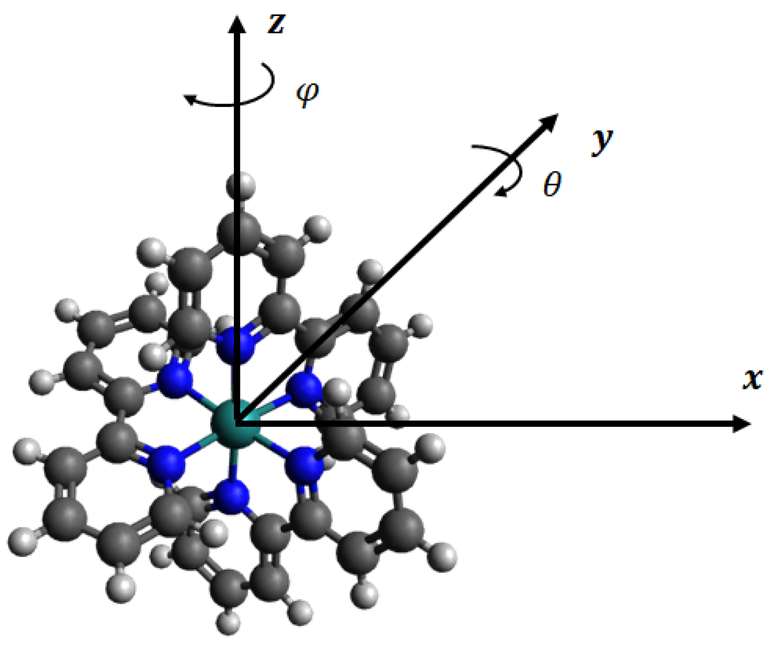
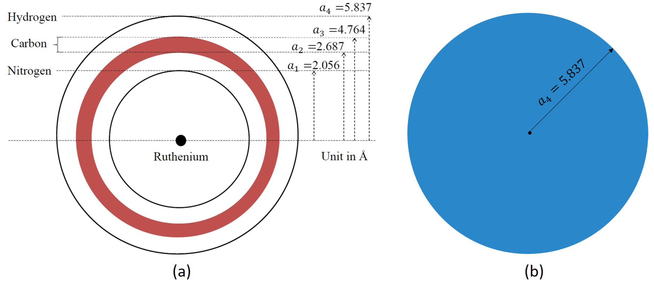
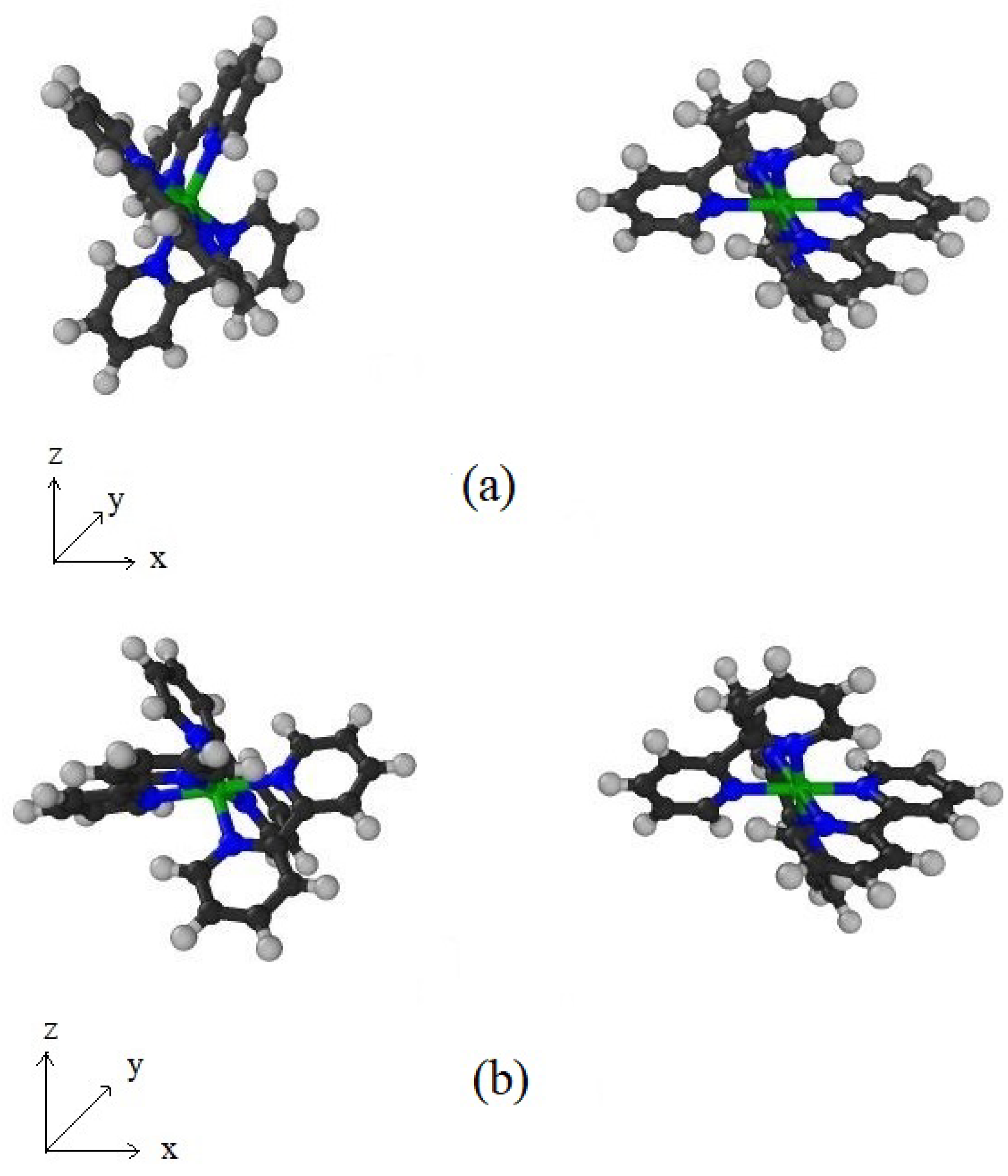
The molecular structure of Ru(bpy)${}_3^{2+}$ is C${}_{30}$H${}_{24}$N${}_6$Ru${}^{2+}$ is shown in Figure 1. The ruthenium (Ru), nitrogen (N), carbon (C), and hydrogen (H) atoms are all radially distributed from the centre, and therefore, as shown in Figure 2a, we may model the molecule as spherical layers of N, C, and H atoms and with the Ru atom located at the centre of the molecule. We observe that C atoms are densely packed between N and H layers. Consequently we assume that the layer of C atoms is modelled as a shell of a certain thickness ℓ.

The radius for each shell is obtained from Avogadro (a molecular editor and visualizer software), where both the bond length and the bond angle are taken into account. As illustrated in Figure 2a, the radii of N and H layers are assumed to be $a_1=2.056$ Å and $a_4=5.837$ Å, respectively, whereas the thickness of the C layer is taken to be $\ell =a_3-a_2=4.764-2.687$ Å.

The mean atomic surface densities of N and H layers, and the mean atomic volume density of the C layer are given by

$${\eta }_N=\frac{6}{4\pi a_1^2}=0.1130{\AA }^{-2},{\eta }_H=\frac{24}{4\pi a_4^2}=0.0561{\AA }^{-2},{\eta }_C=\frac{30}{\left[4\pi (a_3^3-a_2^3)\right]/3}=0.0807{\AA }^{-3},$$

where the Ru(bpy)${}_3^{2+}$ molecule is composed of six N atoms, 24 H atoms, and 30 C atoms, and we subsequently refer to this model as Model I.

Although Model I preserves the spherically symmetric nature of the four atomic types in Ru(bpy)${}_3^{2+}$, a number of parameters are needed to define this model. Accordingly, we consider a second simpler approach for which Ru(bpy)${}_3^{2+}$ is modelled as a solid sphere of radius $a_4=5.837$ Å with mean atomic volume density:

$${\eta }_{Dye}^v=\frac{61}{\left(4\pi a_4^3\right)/3}=0.0732{\AA }^{-3},$$

which we refer to as Model II and this model is shown in Figure 2b.

2.2. Structure of TiO${}_2$

The TiO${}_2$ semiconductor is assumed to be formed from mixed crystals of titanium dioxides, and only atomic proportions of titanium and oxygen are considered. In this paper, we model the TiO${}_2$ molecule as a solid sphere of radius $b=50$ Å. We note that this value is chosen to facilitate the computation in our molecular dynamics simulations since it is large enough as compared to the size of the dye molecule. A value larger than this would require a longer computational time for little significant change from the results presented here. Using $b=50$ Å, the mean volume density of spherical TiO${}_2$ structure becomes

$${\eta }_{Ti{O}_2}=\frac{N_{Ti}+N_O}{\left(4\pi b^3\right)/3}=0.0883{\AA }^{-3},$$

where $N_{Ti}$ and $N_O$ are the numbers of titanium atoms and oxygen atoms, respectively [33,34,35].

2.3. Potential Function and Continuum Approach

In the DSSCs, the dye molecules and the semiconductor are placed in an electrolytic solution. Consequently, they become neutralized and thus we may ignore their electrostatic interactions, and therefore, we only consider the van der Waals interaction here. The Lennard-Jones potential is utilized to quantify the van der Waals interaction energy between two atoms, and it can be written as

$$\mathsf{\Phi }\left(\rho \right)=\frac{-A}{{\rho }^6}+\frac{B}{{\rho }^{12}},$$

(1)

where $A=4ϵ{\sigma }^6$ and $B=4ϵ{\sigma }^{12}$ represent the attractive and the repulsive constants, respectively, $ϵ$ is the well depth, $\sigma$ is the van der Waals diameter, and $\rho$ denotes the distance between the atoms. For the interaction between two molecules using the continuum approach, the total potential energy can be obtained by integrating (1) over the surfaces or volumes of the two molecular structures,

$$E={\eta }_1{\eta }_2{\int }_{{\Sigma }_1}{\int }_{{\Sigma }_2}\left(-\frac{A}{{\rho }^6}+\frac{B}{{\rho }^{12}}\right)d{\Sigma }_{2}d{\Sigma }_1,$$

(2)

where ${\eta }_1$ and ${\eta }_2$ represent either the mean atomic surface densities (when molecules are modelled as surfaces), or the mean atomic volume densities (when molecules are modelled as volumetric structures). Moreover, ${\Sigma }_1$ and ${\Sigma }_2$ are either the surface areas or the volumes of the two molecules. By introducing the notation $I_n$,

$$I_n={\int }_{{\Sigma }_1}{\int }_{{\Sigma }_2}\frac{1}{{\rho }^{2n}}d{\Sigma }_{2}d{\Sigma }_1,n=3,6,$$

(3)

the potential energy given by (2) becomes

$$E={\eta }_1{\eta }_2(-A{I}_3+B{I}_6).$$

(4)

The values of $ϵ$ and $\sigma$ are taken from [36], and the Lennard-Jones constants A and B are calculated which are given in Appendix A.

There are five integrals $I_n$ corresponding to five types of interactions which are needed to be evaluated.

(i)

Single atom interacting with a spherical surface:

Following the work of Cox et al. [27], the two integrals $I_3^S$ and $I_6^S$ can be expressed as

$$\begin{array}{ccc}\hfill I_3^S[a,J_m\left(a\right)]& =& 4\pi a^2[J_3\left(a\right)+2a^2{J}_4\left(a\right)],\hfill \end{array}$$

(5)

$$\begin{array}{ccc}\hfill I_6^S[a,J_m\left(a\right)]& =& 4\pi a^2[5J_6\left(a\right)+80a^2{J}_7\left(a\right)+336a^4{J}_8\left(a\right)+512a^6{J}_9\left(a\right)\hfill \\ & +& 256a^8{J}_{10}\left(a\right)]/5,\hfill \end{array}$$

(6)

where $J_m\left(a\right)=1/{(Z^2-a^2)}^m$, a is a radius of the sphere, and Z denotes the distance between the atom and the centre of the spherical surface.

(ii)

Single atom interacting with a solid sphere:

Analytical expressions for this interaction were derived by Baowan and Thamwattana [32], and are restated here as

$$\begin{array}{ccc}\hfill I_3^V[a,J_m\left(a\right)]& =& 4\pi a^3{J}_3\left(a\right)/3,\hfill \end{array}$$

(7)

$$\begin{array}{ccc}\hfill I_6^V[a,J_m\left(a\right)]& =& 2\pi a^3[30J_6\left(a\right)+216a^2{J}_7\left(a\right)+432a^4{J}_8\left(a\right)+256a^6{J}_9\left(a\right)]/45,\hfill \end{array}$$

(8)

where again $J_m\left(a\right)=1/{(Z^2-a^2)}^m$.

(iii)

Interaction between two spherical surfaces:

By integrating the expressions given in Equations (5) and (6) over another spherical surface, the interaction energy between two spherical surfaces is obtained, given by

$$\begin{array}{ccc}\hfill K_m(a,\tilde{a})& =& {\int }_S{J}_m\left(a\right)dS={\int }_{-\pi }^{\pi }{\int }_0^{\pi }\frac{{\tilde{a}}^{2}sin\varphi }{{({\tilde{a}}^2+2\tilde{a}Zcos\varphi +Z^2-a^2)}^m}d\varphi d\theta \hfill \\ & =& \frac{\tilde{a}\pi }{Z(1-m)}\left\{\frac{1}{{[{(\tilde{a}+Z)}^2-a^2]}^{m-1}}-\frac{1}{{[{(\tilde{a}-Z)}^2-a^2]}^{m-1}}\right\},\hfill \end{array}$$

(9)

where $\tilde{a}$ denotes the radius of the second sphere and Z represents the distance between the centres of the two spheres.

(iv)

Spherical surface interacting with a spherical shell (with finite thickness $\ell =a_3-a_2$):

Again, we integrate the expressions given in Equations (5) and (6) over the spherical shell, which we deduce

$$\begin{array}{ccc}\hfill L_m\left(a\right)& =& {\int }_V{J}_m\left(a\right)dV={\int }_{-\pi }^{\pi }{\int }_0^{\pi }{\int }_{a_2}^{a_3}\frac{r^{2}sin\varphi }{{(r^2+2rZcos\varphi +Z^2-a^2)}^m}drd\varphi d\theta \hfill \\ & =& \frac{\pi }{Z(1-m)}{\int }_{a_2}^{a_3}r\left\{\frac{1}{{[{(r+Z)}^2-a^2]}^{m-1}}-\frac{1}{{[{(r-Z)}^2-a^2]}^{m-1}}\right\}dr.\hfill \end{array}$$

(v)

Spherical surface interacting with a solid sphere:

By integrating the expressions given in Equations (5) and (6) over the solid sphere, we have

$$\begin{array}{ccc}\hfill M_m(a,\tilde{a})& =& {\int }_V{J}_m\left(a\right)dV={\int }_{-\pi }^{\pi }{\int }_0^{\pi }{\int }_0^{\tilde{a}}\frac{r^{2}sin\varphi }{{(r^2+2rZcos\varphi +Z^2-a^2)}^m}drd\varphi d\theta \hfill \\ & =& \frac{\pi }{Z(1-m)}{\int }_0^{\tilde{a}}r\left\{\frac{1}{{[{(r+Z)}^2-a^2]}^{m-1}}-\frac{1}{{[{(r-Z)}^2-a^2]}^{m-1}}\right\}dr.\hfill \end{array}$$

3. Interaction Energies between Dye and Semiconductor

Upon adopting the analytical expressions given in the previous section, the interaction energy between two dye molecules, and between a dye molecule and a TiO${}_2$ structure can be determined. The details are presented in the following subsection.

3.1. Ru(bpy)${}_3^{2+}$–Ru(bpy)${}_3^{2+}$

3.1.1. Model I

In Model I, the Ru atom is assumed to be located at the centre and surrounded by the layers of N, C and H atoms. The interaction between two Ru(bpy)${}_3^{2+}$ molecules can be obtained from summing over all possible interactions, namely

$$E_{M1}=\sum _i\sum _j{E}_{ij},$$

(10)

where i and j represent the atomic species of Ru, N, C and H. The total interaction energies of the two dye molecules are detailed in Appendix B.

3.1.2. Model II

The Ru(bpy)${}_3^{2+}$ molecule is assumed to be a solid sphere of radius $a_4=5.837$ Å, and the interaction energy between two dye molecules can be calculated by

$$E_{M2}={\eta }_{Dye}^v{\eta }_{Dye}^v\left\{-A_{Dye-Dye}{I}_3^V[a_4,M_m(a_4,a_4)]+B_{Dye-Dye}{I}_6^V[a_4,M_m(a_4,a_4)]\right\},$$

(11)

where $I_3^V$ and $I_6^V$ are given in Equations (7) and (8), respectively, and the Lennard-Jones constants A and B are given in Appendix A.

3.2. Ru(bpy)${}_3^{2+}$–TiO${}_2$

3.2.1. Model I

The potential energy between the dye molecule of Model I and a solid sphere of TiO${}_2$ is given by

$${\tilde{E}}_{M1}=\sum _i{E}_{i-Ti{O}_2},$$

(12)

where i refers to either to Ru atom, N, C or H layers. Again, the total interaction energy is detailed in Appendix B.

3.2.2. Model II

The energy arising from the interaction between a solid sphere of the dye molecule and a solid sphere of TiO${}_2$ can be given by

$${\tilde{E}}_{M2}={\eta }_{Dye}^v{\eta }_{Ti{O}_2}\left\{-A_{Dye-Ti{O}_2}{I}_3^V[a_4,M_m(a_4,b)]+B_{Dye-Ti{O}_2}{I}_6^V[a_4,M_m(a_4,b)]\right\},$$

(13)

where the calculation for the attractive A and the repulsive B constants is given in Appendix A.

4. Results and Discussion

To validate the analytical models, we compare our results with molecular dynamics (MD) simulations, which are performed using the LAMMPS Molecular Dynamics Simulator [37,38]. In the simulations, the potential energy of the molecular system is computed using the discrete Lennard-Jones potential,

$$E^{dis}=\sum _{\alpha }\sum _{\beta }4{ϵ}_{\alpha \beta }\left[{\left(\frac{{\sigma }_{\alpha \beta }}{{\rho }_{\alpha \beta }}\right)}^{12}-{\left(\frac{{\sigma }_{\alpha \beta }}{{\rho }_{\alpha \beta }}\right)}^6\right],{\rho }_{\alpha \beta }<{\rho }_c,$$

where ${\rho }_{\alpha \beta }$ represents the distance between atom $\alpha$ and atom $\beta$ of two molecules. The values of the Lennard-Jones parameters used in MD simulations are assumed to be the same to those used in the continuum models, which are given in

Table A1. Lennard-Jones parameters used here.

Atomic Type	$\mathit{ϵ}$ (kcal/mol)	$\mathit{\sigma }$ (Å)
Ru	0.056	2.6397
N	0.069	3.2607
C	0.105	3.4309
H	0.044	2.5711
Ti	0.017	2.8286
O	0.060	3.1181

. Only the atoms at distances less than the cut-off radius ${\rho }_c=22$ Å are assumed to interact with each other.

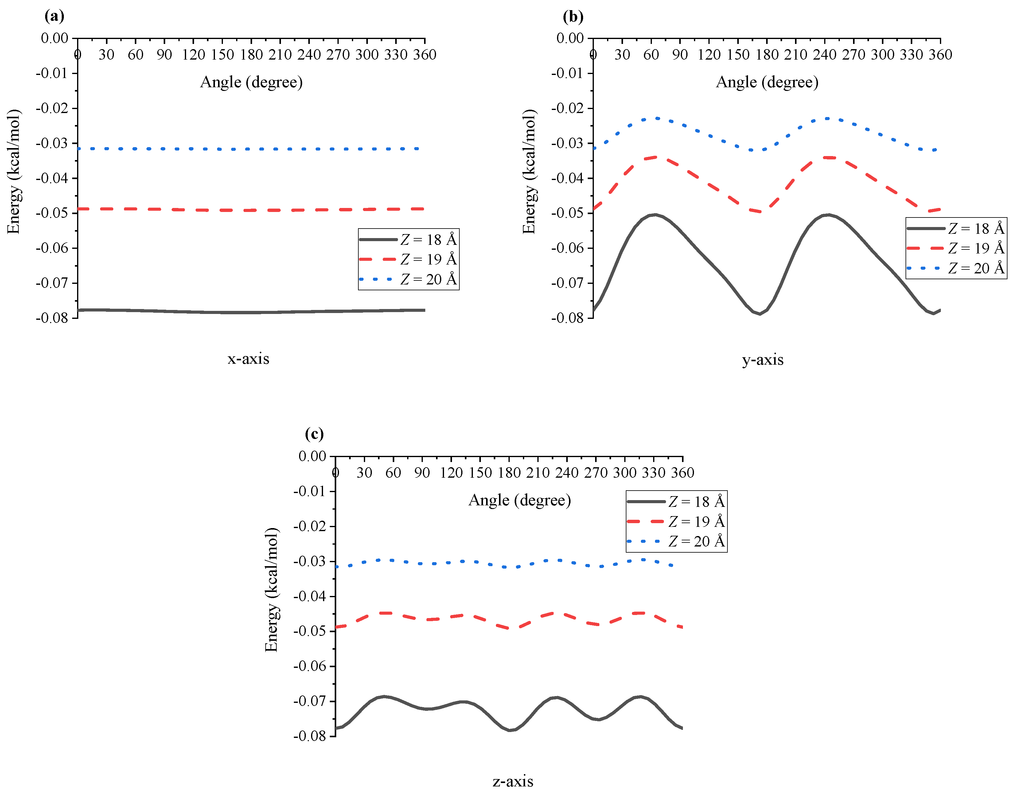
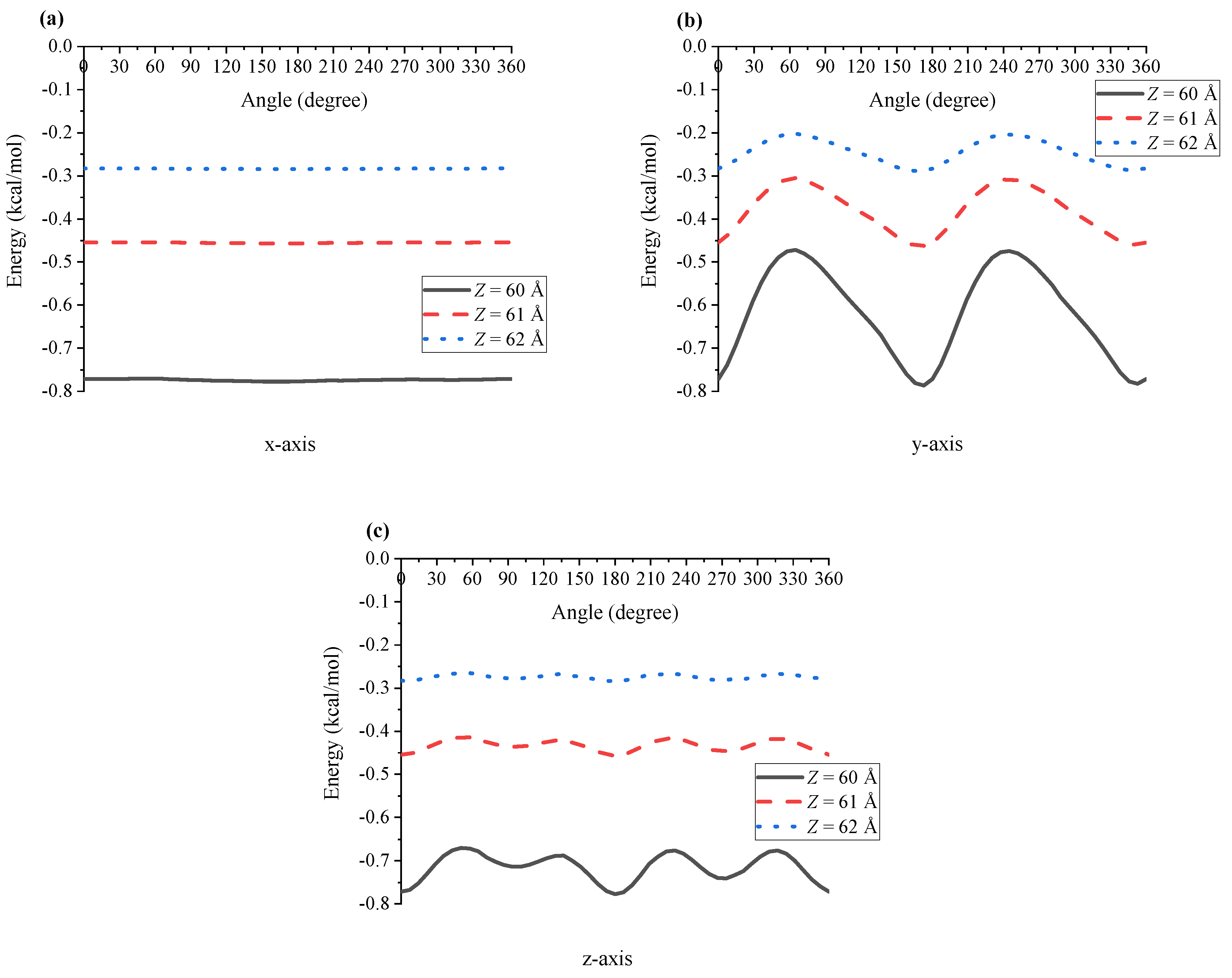
In the case of the interaction between two Ru(bpy)${}_3^{2+}$ molecules, one of the molecules is assumed to be fixed and the other is at distance Z from the first molecule, where Z is defined as the centre-to-centre distance.However, as shown in Figure 1, the dye molecule is not perfectly symmetric, and therefore to calculate the interaction energy, we first rotate the molecule about its three axes to compute the energy at different angles and then take an average to obtain the final result. In Figure 3, we plot the interaction energy between two dye molecules when the first molecule rotates about $x-$, $y-$ and $z-$axis for different values of Z. It can be seen that the energy is smooth when the first dye molecule rotates only about the x-axis. This is because the configuration of the dye is almost symmetric about this axis, and the energy fluctuation is larger when the molecule rotates about the y- and z-axis, which demonstrates a less symmetric structure of the dye in these directions. Since the molecule is symmetric in the $x-$direction, we only need to consider the rotation of the molecule about the $y-$ and $z-$ axis, which corresponds respectively to the rotation angles $\theta$ and $\varphi$, defined in Figure 1.

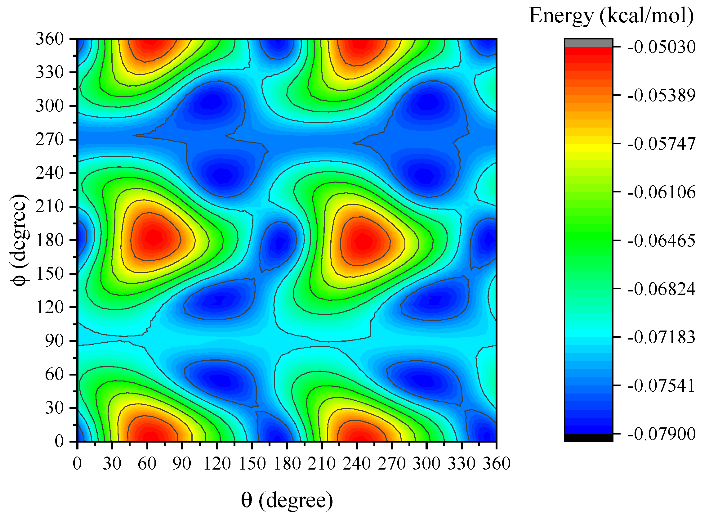
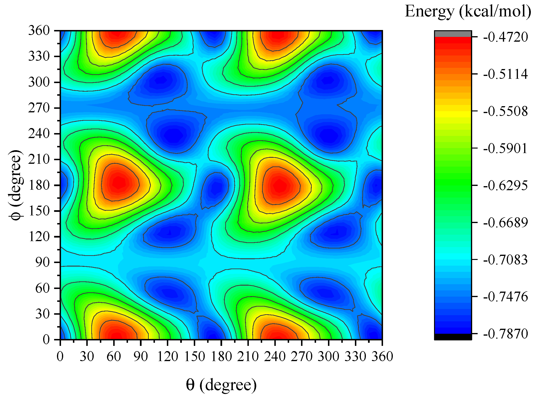
Contours for the interaction energy between two dye molecules at $Z=18$ Å are plotted in Figure 4. The horizontal and vertical axes are the rotational angles of the second molecule about the y- and z-axis, respectively. We observe that the peak energy for the interaction is obtained for $\theta ={64.8}^{\circ }$ and $\varphi ={180}^{\circ }$ where $E_{Dye-Dye}^{dis}=-0.05040$ kcal/mol. The variation of the energy under the various rotations of the dye molecule reflects the face that Ru(bpy)${}_3^{2+}$ is not perfectly spherical (see Figure A1 in Appendix C).

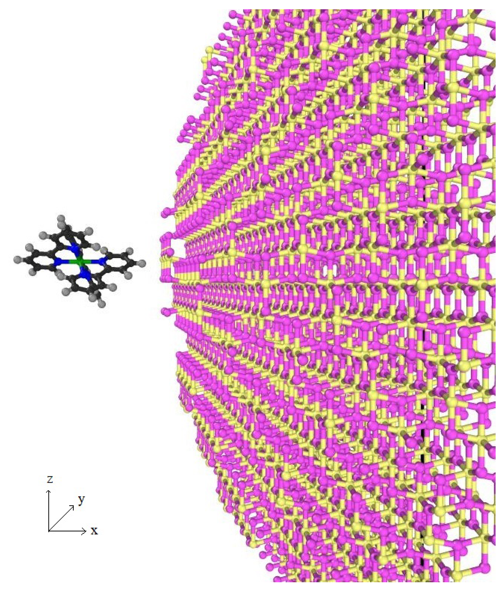
For the interaction between a dye molecule and a sphere of TiO${}_2$, in the MD simulation, the dye molecule is rotated and moved toward the fixed TiO${}_2$ sphere, assuming that the radius of the TiO${}_2$ sphere is 50 Å (see Figure A2 in Appendix C). The energy profiles for the dye molecule, rotated in the three directions, interacting with TiO${}_2$ are depicted in Figure 5. We see that the energy exhibits fluctuations similar to those of the two dye molecules but with higher energy values. As shown in Figure 6 for $Z=60$ Å, two configurations corresponding to $\theta ={64.8}^{\circ }$ and $\varphi ={180}^{\circ }$, and $\theta ={122.4}^{\circ }$ and $\varphi ={129.6}^{\circ }$ give the highest energy of $-0.47335$ kcal/mol and the lowest energy of $-0.78032$ kcal/mol, respectively.

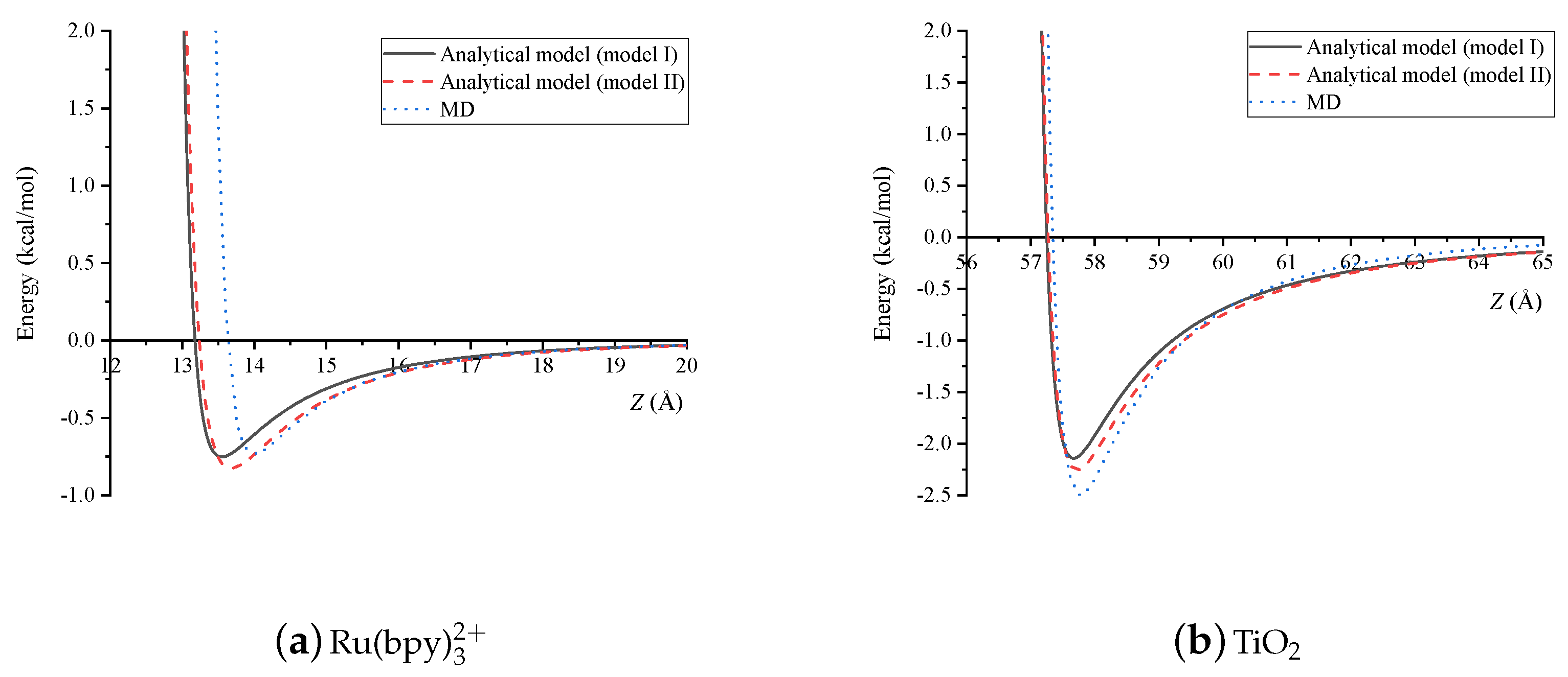
Since the dye molecule is not perfectly symmetric, the energy values obtained from the analytical models, under the assumption of spherical dye molecule, are compared with averaged values obtained from the MD simulations. For the dye-dye interaction, the distance of the two molecules is varied from 13 Å to 20 Å and the interaction energy is recorded and plotted in Figure 7a. Similarly, comparison between the analytical models and the MD simulation for a dye molecule and a TiO${}_2$ is shown in Figure 7b. Some discrete values of the interaction energy for the two cases are also reported in

Table 1. Energies for dye-dye and dye-TiO${}_2$ interactions of Model I ($E_{M1}$), Model II ($E_{M2}$), and MD ($E^{MD}$).

Z (Å)	${\mathit{E}}_{\mathit{M}1}$ (kcal/mol)	${\mathit{E}}_{\mathit{M}2}$ (kcal/mol)	${\mathit{E}}_{\mathit{Dye}-\mathit{Dye}}^{\mathit{MD}}$ (kcal/mol)
14	−0.60734	−0.73692	−0.73387
15	−0.31122	−0.38330	−0.38954
16	−0.17442	−0.20862	−0.20240
17	−0.10536	−0.12263	−0.11636
18	−0.06718	−0.07649	−0.07140
Z (Å)	${\tilde{E}}_{M1}$ (kcal/mol)	${\tilde{E}}_{M2}$ (kcal/mol)	$E_{Dye-Ti{O}_2}^{MD}$ (kcal/mol)
57.75	−2.12208	−2.25520	−2.50002
59.5	−0.87185	−0.94729	−0.92917
60	−0.69583	−0.75015	−0.70249
60.5	−0.56526	−0.60502	−0.54128
61	−0.46601	−0.49565	−0.42338

. It is observed that the values of the interaction energies obtained by the continuum models are close to those obtained by the MD simulation. We may conclude that the Ru(bpy)${}_3^{2+}$ dye molecule can be modelled either as a spherical shell or as a solid sphere in order to study the interaction and the arrangement of two dye molecules, and between the dye molecule and the TiO${}_2$ structure.

We note that the atoms in the continuum model are assumed to be smeared over the molecule which is different from MD where the discrete positions of each atom are required. These differences lead to the different values for the energy between the continuum models and the MD simulation. On the other hand, the continuum approximation for the atoms has only a minor impact on the energy of the dye molecule interacting with TiO${}_2$ because a semiconductor with the radius $b=50$ Å is much larger than the size of the dye molecule. Hence, the energy profiles of the continuum models are hardly different from the discrete model in the case of the dye-TiO${}_2$ interaction as illustrated in Figure 7b.

Furthermore, we focus on the equilibrium distance which is defined by $Z_{min}$ arising from the interaction between two molecules. This position gives rise to the minimum interaction energy implying the equilibrium configuration. The lowest value of the interaction energy indicates the location where the two nano-objects are most stable. The distance where the molecules can overcome the energy barrier and attract each other is also investigated and denoted by $Z_0$. Therefore, the dye molecule can be attached to the other dye molecules or to the TiO${}_2$ semiconductor when $Z\ge Z_0$.

Table 2. Values of $Z_0$ and $Z_{min}$ for continuum and discrete models.

Dye-Dye	${\mathit{Z}}_0$ (Å)	${\mathit{Z}}_{\mathit{min}}$ (Å)
Model I	13.18	13.54
Model II	13.24	13.66
MD	13.52	14.00
Dye-TiO${}_2$	$Z_0$ (Å)	$Z_{min}$ (Å)
Model I	57.25	57.68
Model II	57.27	57.72
MD	57.34	57.75

shows the numerical values of $Z_0$ and $Z_{min}$ for the continuum and the discrete models. We comment that the Lennard-Jones potential appears not to give an accurate prediction of the energy level when the molecules are at a very short distance apart. This is a limitation of the Lennard-Jones potential that is shared by other currently-used potentials, and all molecular level models adopting the Lennard-Jones potential are not able to accurately predict short-range interactions between molecules. The energy value at $Z<Z_0$ shown in Figure 7 is an estimation from the molecular-level model and it should be taken only as a reference value. For a more precise evaluation for short-ranged interactions, ab-initio calculations at sub-atomic scale are required, which presents an opportunity for future research.

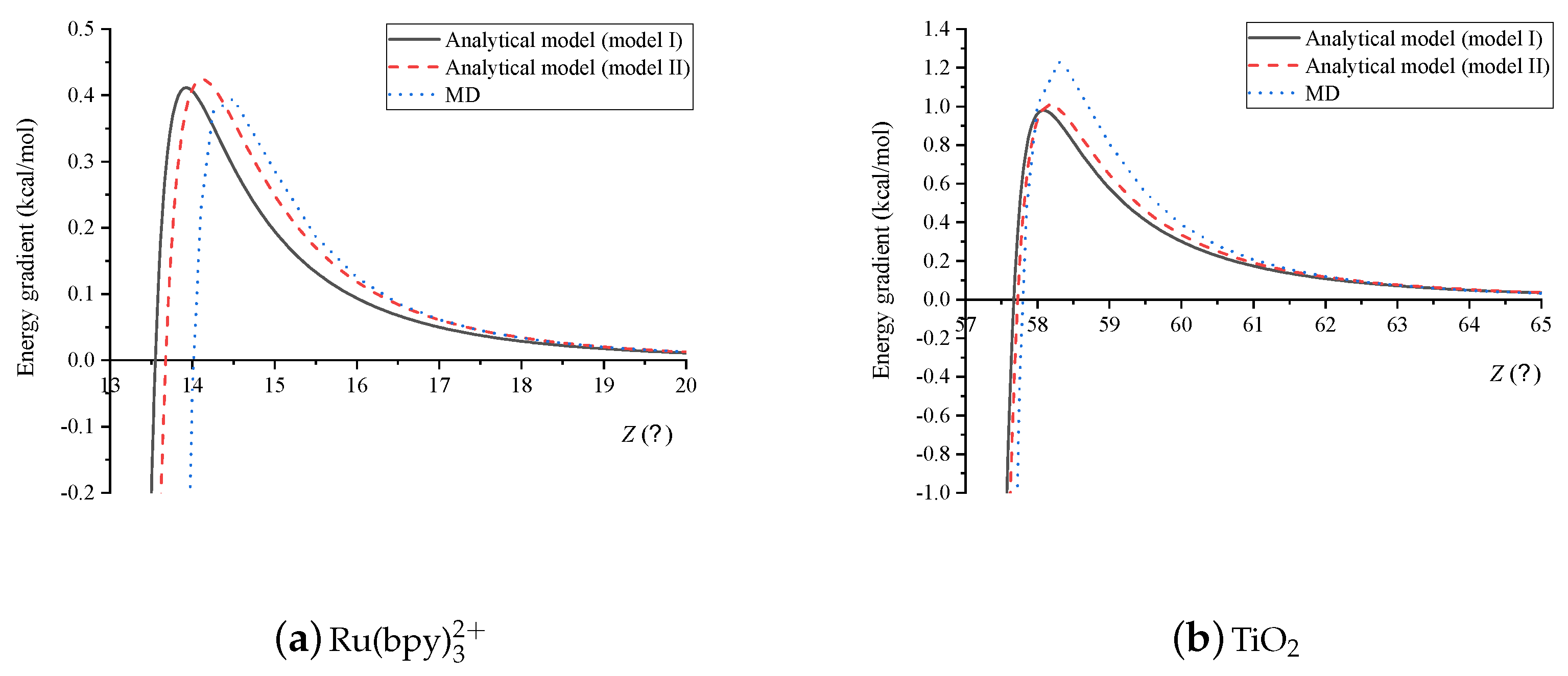
In Figure 8a,b we plot the energy gradients corresponding to the two interactions shown in Figure 7a,b. We note that the critical distance Z where the energy is minimum in Figure 7a,b corresponding to the values of $Z_{min}$ where the energy gradient is zero in Figure 8a,b, respectively. We also observe a strong increase in energy near the equilibrium, and the rate of the change of the energy decreases as the distance between two molecules increases.

5. Summary

Based on the structural materials of dye-sensitized solar cells (DSSCs), this paper studies the interactions of two dye molecules and between the dye molecule and the TiO${}_2$ semiconductor. We use the continuum approach and the Lennard-Jones potential to evaluate the molecular interaction energy of the systems to determine analytical expressions for the interaction energy.

In addition, MD simulations are performed to investigate the energy behaviour of two dye molecules and the dye molecule interacting with the semiconductor TiO${}_2$. The results obtained from the simulations demonstrate that the Ru(bpy)${}_3^{2+}$ dye molecule is not a perfectly spherical. However, both a spherical shell and a densely packed sphere provide a good approximation to model the dye molecule as numerically indicated in Table 1. We also find the minimum distance where the two nanoparticles begin to attract each other and the equilibrium distance where the two molecules are most stable. The present work provides an insight and understanding of the Ru(bpy)${}_3^{2+}$ dye molecule interacting with TiO${}_2$ structure and a basic tool for modelling these components, which is crucial for the further development of DSSCs. Future work in this area includes the development of a more robust benchmark study (e.g., a full ab initio molecular dynamics study) for the quantitative and qualitative validations of the analytical models.

References

- Maldon, B.; Thamwattana, N. An analytical solution for charge carrier densities in dye-sensitized solar cells. J. Photochem. Photobiol. A Chem. 2019, 370, 41–50. [Google Scholar] [CrossRef]
- Maldon, B.; Thamwattana, N.; Edwards, M. Exploring nonlinear diffusion equations for modelling dye-Sensitized solar cells. Entropy 2020, 22, 248. [Google Scholar] [CrossRef] [Green Version]
- Kalyanasundaram, K. Photophysics, photochemistry and solar energy conversion with tris(bipyridyl)ruthenium(II) and its analogues. Coord. Chem. Rev. 1982, 46, 159–244. [Google Scholar] [CrossRef]
- Juris, A.; Balzani, V. Ru(II) polypyridine complexes: Photophysics, photochemistry, electrochemistry, and chemiluminescence. Coord. Chem. Rev. 1988, 84, 85–277. [Google Scholar] [CrossRef]
- Campagna, S.; Puntoriero, F.; Nastasi, F.; Bergamini, G.; Balzani, V. Photochemistry and photophysics of coordination compounds: Ruthenium. Top. Curr. Chem. 2007, 280, 117–214. [Google Scholar]
- Seidel, R.; Faubel, M.; Winter, B.; Blumberger, J. Single-ion reorganization free energy of aqueous Ru(bpy) and Ru(H2O) from photoemission spectroscopy and density functional molecular dynamics simulation. J. Am. Chem. Soc. 2009, 131, 16127–16137. [Google Scholar] [CrossRef]
- Diamantis, P.; Gonthier, J.F.; Tavernelli, I.; Rothlisberg, U. Study of the redox properties of singlet and triplet tris(2,2′-bipyridine)ruthenium(II) ([Ru(bpy)3]2+) in aqueous solution by full quantum and mixed quantum/classical molecular dynamics simulations. J. Phys. Chem. B 2014, 118, 3950–3959. [Google Scholar] [CrossRef]
- Duan, L.; Xu, Y.; Zhang, P.; Wang, M.; Sun, L. Visible light-driven water oxidation by a molecular ruthenium catalyst in homogeneous system. Inorg. Chem. 2010, 49, 209–215. [Google Scholar] [CrossRef]
- Xu, Y.; Duan, L.; Tong, L.; Åkermark, B.; Sun, L. Visible light-driven water oxidation catalyzed by a highly efficient dinuclear ruthenium complex. Chem. Commun. 2010, 46, 6506–6508. [Google Scholar] [CrossRef]
- Kärkäs, M.D.; Åkermark, T.; Johnston, E.V.; Karim, S.R.; Laine, T.M.; Lee, B.L.; Åkermark, T.; Privalov, T.; Åkermark, B. Water oxidation by single-site ruthenium complexes: Using ligands as redox and proton transfer mediators. Angew. Chem. Int. Ed. 2012, 51, 11589–11593. [Google Scholar] [CrossRef]
- Lewandowska-Andralojc, A.; Polyansky, D.E.; Zong, R.; Thummel, R.P.; Fujita, E. Enabling light-driven water oxidation via a low-energy RuIV=O intermediate. Phys. Chem. Chem. Phys. 2013, 15, 14058–14068. [Google Scholar] [CrossRef]
- Kärkäs, M.D.; Verho, O.; Johnston, E.V.; Åkermark, B. Artificial photosynthesis: Molecular systems for catalytic water oxidation. Chem. Rev. 2014, 114, 11863–12001. [Google Scholar] [CrossRef]
- Shylin, S.I.; Pavliuk, M.V.; D’Amario, L.; Fritsky, I.O.; Berggren, G. Photoinduced hole transfer from tris(bipyridine)ruthenium dye to a high-valent iron-based water oxidation catalyst. Faraday Discuss. 2019, 215, 162–174. [Google Scholar] [CrossRef] [Green Version]
- Cassone, G.; Calogero, G.; Sponer, J.; Saija, F. Mobilities of iodide anions in aqueous solutions for applications in natural dye-sensitized solar cells. Phys. Chem. Chem. Phys. 2018, 20, 13038–13046. [Google Scholar] [CrossRef]
- Cassone, G.; Chillé, D.; Foti, C.; Giuffré, O.; Ponterio, R.C.; Sponer, J.; Saija, F. Stability of hydrolytic arsenic species in aqueous solutions: As3+vs. As5+. Phys. Chem. Chem. Phys. 2018, 20, 23272–23280. [Google Scholar] [CrossRef]
- Park, N.G.; van de Lagemaat, J.; Frank, A.J. Comparison of dye-sensitized rutile- and anatase-based TiO2 solar cells. J. Phys. Chem. B 2000, 104, 8989–8994. [Google Scholar] [CrossRef] [Green Version]
- Van de Lagemaat, J.; Benkstein, K.D.; Frank, A.J. Relation between Particle Coordination Number and Porosity in Nanoparticle Films: Implications to Dye-Sensitized Solar Cells. J. Phys. Chem. B 2001, 105, 12433–12436. [Google Scholar] [CrossRef]
- Benkstein, K.D.; Kopidakis, N.; van de Lagemaat, J.; Frank, A.J. Influence of the Percolation Network Geometry on Electron Transport in Dye-Sensitized Titanium Dioxide Solar Cells. J. Phys. Chem. B 2003, 107, 7759–7767. [Google Scholar] [CrossRef]
- Tan, B.; Wu, Y. Dye-sensitized solar cells based on anatase TiO2 nanoparticle/nanowire composites. J. Phys. Chem. B 2006, 110, 15932–15938. [Google Scholar] [CrossRef]
- Angelis, F.D.; Fantacci, S.; Selloni, A. Alignment of the dye’s molecular levels with the TiO2 band edges in dye-sensitized solar cells: A DFT-TDDFT study. Nanotechnology 2008, 19, 424002. [Google Scholar] [CrossRef]
- Mosconi, E.; Yum, J.H.; Kessler, F.; García, C.J.G.; Zuccaccia, C.; Cinti, A.; Nazeeruddin, M.K.; Grätzel, M.; Angelis, F.D. Cobalt electrolyte/dye interactions in dye-sensitized solar cells: A combined computational and experimental study. J. Am. Chem. Soc. 2012, 134, 19438–19453. [Google Scholar] [CrossRef] [PubMed]
- Fazli, F.I.M.; Ahmad, M.K.; Soon, C.F.; Nafarizal, N.; Suriani, A.B.; Mohamed, A.; Mamat, M.H.; Malek, M.F.; Shimomura, M.; Murakami, K. Dye-sensitized solar cell using pure anatase TiO2 annealed at different temperatures. Optik 2017, 140, 1063–1068. [Google Scholar] [CrossRef]
- Liu, J.; Luo, J.; Yang, W.; Wang, Y.; Zhu, L.; Xu, Y.; Tang, Y.; Hu, Y.; Wang, C.; Chen, Y.; et al. Synthesis of single-crystalline anatase TiO2 nanorods with high-performance dye-sensitized solar cells. J. Mater. Sci. Technol. 2015, 31, 106–109. [Google Scholar] [CrossRef]
- Chu, L.; Qin, Z.; Zhang, Q.; Chen, W.; Yang, J.; Yang, J.; Li, X. Mesoporous anatase TiO2 microspheres with interconnected nanoparticles delivering enhanced dye-loading and charge transport for efficient dye-sensitized solar cells. Appl. Surf. Sci. 2016, 360, 634–640. [Google Scholar] [CrossRef]
- Cui, Y.; He, X.; Zhu, M.; Li, X. Preparation of anatase TiO2 microspheres with high exposure (001) facets as the light-scattering layer for improving performance of dye-sensitized solar cells. J. Alloys Compd. 2017, 694, 568–573. [Google Scholar] [CrossRef]
- Girifalco, L.A.; Hodak, M.; Lee, R.S. Carbon nanotubes, buckyballs, ropes, and a universal graphitic potential. Phys. Rev. B 2000, 62, 13104–13110. [Google Scholar] [CrossRef]
- Cox, B.J.; Thamwattana, N.; Hill, J.M. Mechanics of atoms and fullerenes in single-walled carbon nanotubes. I. Acceptance and suction energies. Proc. R. Soc. A 2007, 463, 461–476. [Google Scholar] [CrossRef]
- Hilder, T.M.; Hill, J.M. Continuous versus discrete for interacting carbon nanostructures. J. Phys. A Math. Theor. 2007, 40, 3851–3868. [Google Scholar] [CrossRef]
- Baowan, D.; Cox, B.J.; Hill, J.M. Instability of C60 fullerene interacting with lipid bilayer. J. Mol. Model. 2012, 18, 549–557. [Google Scholar] [CrossRef]
- Rahmat, F.; Thamwattana, N.; Cox, B.J. Modelling peptide nanotubes for artificial ion channels. Nanotechnology 2011, 22, 445707. [Google Scholar] [CrossRef]
- Baowan, D.; Peuschel, H.; Kraegeloh, A.; Helms, V. Energetics of liposomes encapsulating silica nanoparticles. J. Mol. Model. 2013, 19, 2459–2472. [Google Scholar] [CrossRef] [PubMed]
- Baowan, D.; Thamwattana, N. Modelling selective separation of trypsin and lysozyme using mesoporous silica. Microporous Mesoporous Mater. 2013, 176, 209–214. [Google Scholar] [CrossRef]
- Diebold, U. The surface science of titanium dioxide. Surf. Sci. Rep 2003, 48, 53–229. [Google Scholar] [CrossRef]
- Wang, Y.; Zhang, R.; Li, J.; Li, L.; Lin, S. First-principles study on transition metal-doped anatase TiO2. Nanoscale Res. Lett. 2014, 9, 46. [Google Scholar] [CrossRef] [PubMed] [Green Version]
- Jia, J.; Yamamoto, H.; Okajima, T.; Shigesato, Y. On the crystal structural control of sputtered TiO2 thin films. Nanoscale Res. Lett. 2016, 11, 324. [Google Scholar] [CrossRef] [Green Version]
- Rappé, A.K.; Casewit, C.J.; Colwell, K.S.; III, W.A.G.; Skiff, W.M. UFF, a Full Periodic Table Force Field for Molecular Mechanics and Molecular Dynamics Simulations. J. Am. Chem. Soc. 1992, 114, 10024–10035. [Google Scholar] [CrossRef]
- LAMMPS Molecular Dynamics Simulator. Available online: https://lammps.sandia.gov (accessed on 1 July 2019).
- Plimpton, S. Fast Parallel Algorithms for Short-Range Molecular Dynamics. J. Comp. Phys. 1995, 117, 1–19. [Google Scholar] [CrossRef] [Green Version]
- Hirschfelder, J.O.; Curtiss, C.F.; Bird, R.B. Molecular Theory of Gases and Liquids; Wiley: New York, NY, USA, 1954. [Google Scholar]
Figure 1.
Three-dimensional structure of Ru(bpy). The ruthenium atom (Ru) is at the centre in green; six nitrogen atoms (N) in blue; carbon atoms (C) in black, and hydrogen atoms (H) in grey.
Figure 2.
Two models for Ru(bpy) molecule: (a) Model I: Spherical layers and (b) Model II: Solid sphere.
Figure 3.
Interaction energy between two dye molecules when first molecule rotates about (a) x-, (b) y-, and (c) z-axis.
Figure 4.
Contour plot of energy against and for the interaction between two dye molecules.
Figure 5.
Interaction energy between dye molecule and TiO when dye molecule rotates about (a) x-axis, (b) y-axis, and (c) z-axis.
Figure 6.
Contour plot of energy against and for interaction between dye molecule and TiO.
Figure 7.
Interaction energy between (a) two dye molecules and (b) dye molecule interacting with TiO molecule obtained from continuum Models I and II, and from MD simulation.
Figure 8.
Energy gradient between (a) two dye molecules and (b) dye molecule interacting with TiO molecule obtained from continuum Models I and II, and from MD simulation.