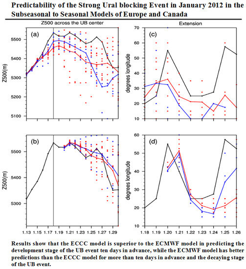
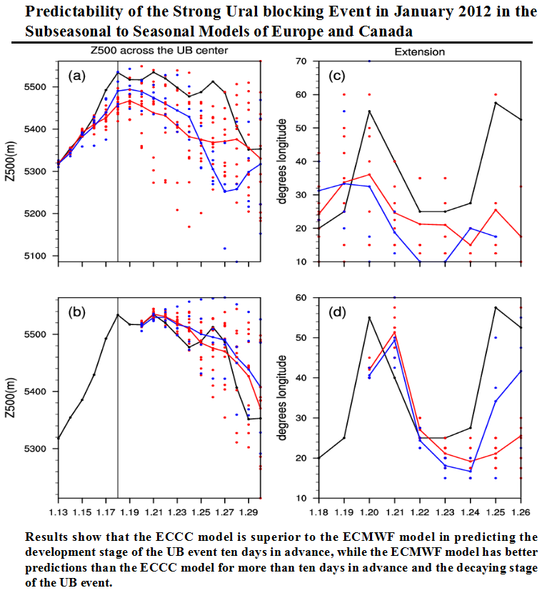
Predictability of the Strong Ural blocking Event in January 2012 in the Subseasonal to Seasonal Models of Europe and Canada


 , ,
, ,
Abstract
:
1. Introduction
2. Data and Methods
2.1. Data
2.2. Detection of Blocking
2.3. Diagnostic Equations
3. Simulation of the Evolution of UB Event
4. Characteristics and Dynamic–Thermodynamic Structure of UB Event
4.1. Characteristics
4.2. Dynamic and Thermodynamic Structure
5. Discussion
6. Summary
Author Contributions
Funding
Acknowledgments
Conflicts of Interest
References
- Tibaldi, S.; Molteni, F. On the operational predictability of blocking. Tellus 1990, 42, 343–365. [Google Scholar] [CrossRef] [Green Version]
- Barriopedro, D.; García-Herrera, R.; Lupo, A.R.; Hernández, E.A. Climatology of Northern Hemisphere blocking. J. Clim. 2006, 19, 1042–1063. [Google Scholar] [CrossRef] [Green Version]
- Wu, M.C.; Leung, W.H. Efect of ENSO on the Hong Kong winter season. Atmos. Sci. Lett. 2009, 10, 94–101. [Google Scholar] [CrossRef]
- Wang, B.; Wu, Z.; Chang, C.P.; Liu, J.; Li, J.; Zhou, T. Another look at interannual-to-interdecadal variations of the East Asian winter monsoon: The northern and southern temperature modes. J. Clim. 2010, 23, 1495–1512. [Google Scholar] [CrossRef] [Green Version]
- Cheung, H.N.; Zhou, W.; Mok, H.Y.; Wu, M.C. Relationship between Ural-Siberian blocking and the East Asian winter monsoon in relation to the Arctic Oscillation and El Niño-Southern Oscillation. J. Clim. 2012, 25, 4242–4257. [Google Scholar] [CrossRef]
- Cheung, H.N.; Zhou, W.; Lee, S.M.; Tong, H.W. Interannual and interdecadal variability of the number of cold days in Hong Kong and their relationship with large-scale circulation. Mon. Weather Rev. 2015, 143, 1438–1454. [Google Scholar] [CrossRef]
- Qiao, S.; Zou, M.; Cheung, H.N.; Dong, W. Predictability of the wintertime 500 hPa geopotential height over Ural-Siberia in the NCEP climate forecast system. Clim. Dyn. 2020, 54, 1591–1606. [Google Scholar] [CrossRef]
- Tao, S. A cold wave in East Asia during a period of blocking decaying. Act Meteorol. Sin. 1957, 28, 63–74. (In Chinese) [Google Scholar]
- Joung, C.H.; Hitchman, M.H. On the role of successive downstream development in East Asian polar air outbreaks. Mon. Weather Rev. 1982, 110, 1224–1237. [Google Scholar] [CrossRef] [Green Version]
- Takaya, K.; Nakamura, H. Mechanisms of intraseasonal ampli-fication of the cold Siberian high. J. Atmos. Sci. 2005, 62, 4423–4440. [Google Scholar] [CrossRef]
- Takaya, K.; Nakamura, H. Geographical dependence of upper-level blocking formation associated with intraseasonal amplification of the Siberian high. J. Atmos. Sci. 2005, 62, 4441–4449. [Google Scholar] [CrossRef]
- Lu, M.-M.; Chang, C.-P. Unusual late-season cold surges during the 2005 Asian winter monsoon: Roles of Atlantic blocking and the Central Asian anticyclone. J. Clim. 2009, 22, 5205–5217. [Google Scholar] [CrossRef]
- Gong, Z.; Feng, G.; Ren, F.; Li, J. A regional extreme low temperature event and its main atmospheric contributing factors. Theor. Appl. Clmatol. 2014, 117, 195–206. [Google Scholar] [CrossRef]
- Gong, Z.; Wang, X.; Ren, F.; Feng, G. The Euro-Asia height positive anomalies character and its probable influence on regional extreme low-temperature events in winter in China. Chin. J. Atmos. Sci. 2013, 37, 1274–1286. (In Chinese) [Google Scholar]
- Tao, S.Y.; Wei, J. Severe snow and freezing-rain in January 2008 in the southern China. Clim. Environ. Res. 2008, 13, 337–350. (In Chinese) [Google Scholar]
- Ding, Y.H.; Wang, Z.Y.; Song, Y.F.; Zhang, J. Causes of the unprecedented freezing disaster in January 2008 and its possible association with the global warming. J. Meteorol. Res. 2008, 66, 808–825. (In Chinese) [Google Scholar]
- Li, Y.; Wang, S.G.; Jin, R.H.; Wang, J.Y.; Li, J.P. Abnormal characteristics of blocking high during durative low temperature, snowfall and freezing weather in southern China. Plateau Meteorol. 2012, 31, 94–101. (In Chinese) [Google Scholar]
- Qiao, S.; Gong, Z.; Feng, G.; Qian, Z. Relationship between cold winters over northern Asia and the subsequent hot summers over mid-lower reaches of the Yangtze River valley under global warming. Atmos. Sci. Lett. 2015, 16, 479–484. [Google Scholar] [CrossRef]
- Gao, S.T.; Zhu, W.M.; Dong, M. Eddy-mean flow interaction in atmospheric low-frequency variation (blocking situation). Act Meteorol. Sin. 1998, 56, 665–680. (In Chinese) [Google Scholar]
- Tyrlis, E.; Hoskins, B.J. The morphology of Northern Hemisphere blocking. J. Atmos. Sci. 2008, 65, 1653–1665. [Google Scholar] [CrossRef]
- Luo, D.; Zhou, W.; Wei, K. Dynamics of eddy-driven North Atlantic Oscillations in a localized shifting jet: Zonal structure and downstream blocking. Clim. Dyn. 2010, 34, 73–100. [Google Scholar] [CrossRef]
- Tracton, M.S. Predictability and its relationship to scale interaction processes in blocking. Mon. Weather Rev. 1990, 118, 1666–1695. [Google Scholar] [CrossRef] [Green Version]
- Tibaldi, S.; Tosi, E.; Navarra, A.; Pedulli, L. Northern and Southern Hemisphere seasonal variability of blocking frequency and predictability. Mon. Weather Rev. 1994, 122, 1971–2003. [Google Scholar] [CrossRef] [Green Version]
- Tibaldi, S.; Ruti, P.; Tosi, E.; Maruca, M. Operational predictability of winter blocking at ECMWF: An update. Ann. Geophys. 1995, 13, 305–317. [Google Scholar]
- Colucci, S.J.; Baumhefner, D.P. Numerical prediction of the onset of blocking: A case study with forecast ensembles. Mon. Weather Rev. 1998, 126, 773–784. [Google Scholar] [CrossRef]
- D’ Andrea, F.; Tibaldi, S.; Blackburn, M.; Boer, G.; Déqué, M.; Dix, M.R.; Dugas, B.; Ferranti, L.; Iwasaki, T.; Kitoh, A.; et al. Northern Hemisphere atmospheric blocking as simulated by 15 atmospheric general circulation models in the period 1979–1988. Clim. Dyn. 1998, 14, 385–407. [Google Scholar] [CrossRef]
- Scaife, A.A.; Woollings, T.; Knight, J.; Martin, G.; Hinton, T. Atmospheric blocking and mean biases in climate models. J. Clim. 2010, 23, 6143–6152. [Google Scholar] [CrossRef] [Green Version]
- Guan, X.D.; Ma, J.R.; Huang, J.P.; Huang, R.X.; Zhang, L.; Ma, Z.G. Impact of oceans on climate change in drylands. Sci. China Earth Sci. 2019, 62, 891–908. [Google Scholar] [CrossRef]
- Barnes, E.A.; Slingo, J.; Woollings, T. A methodology for the comparison of blocking climatologies across indices, models, and climate scenarios. Clim. Dyn. 2012, 38, 2467–2481. [Google Scholar] [CrossRef]
- Giacomo, M.; Hoskins, B.J.; Woollings, T. Winter and summer Northern Hemisphere blocking in CMIP5 models. J. Clim. 2013, 26, 7044–7059. [Google Scholar]
- Jia, X.; Yang, S.; Song, W.; He, B. Prediction of wintertime Northern Hemisphere blocking by the NCEP Climate Forecast System. J. Meteorol. Res. 2014, 28, 76–90. [Google Scholar] [CrossRef]
- World Meteorological Organization. Cold Spell in Europe and Asia in Late Winter 2011/2012. 2012. Available online: https://www.wmo.int/pages/mediacentre/news/documents/dwd (accessed on 8 March 2012).
- Lan, X.Q.; Chen, W. Strong cold weather event over Eurasia during the winter of 2011/2012 and a downward Arctic Oscillation signal from the stratosphere. Chin. J. Atmos. Sci. 2013, 37, 863–872. (In Chinese) [Google Scholar]
- Wu, B.; Yang, K.; Francis, J.A. A cold event in Asia during January–February 2012 and its possible association with Arctic sea ice loss. J. Clim. 2017, 30, 7971–7990. [Google Scholar] [CrossRef]
- Vitart, F.; Ardilouze, C.; Bonet, A.; Brookshaw, A.; Chen, M.; Codorean, C.; Zhang, L. The subseasonal to seasonal (S2S) prediction project database. Bull. Am. Meteorol. Soc. 2017, 98, 163–173. [Google Scholar] [CrossRef]
- Quinting, J.F.; Vitart, F. Representation of synoptic-scale Rossby wave packets and blocking in the S2S prediction project database. Geophys. Res. Lett. 2019, 46, 1070–1078. [Google Scholar] [CrossRef]
- Kalnay, E.; Kanamitsu, M.; Kistler, R.; Collins, W.; Deaven, D.; Gandin, L.; Iredell, M.; Saha, S.; White, G.; Woolen, J.; et al. The NCEP/NCAR 40-year reanalysis project. Bull. Am. Meteorol. Soc. 1996, 77, 437–471. [Google Scholar] [CrossRef] [Green Version]
- Pyper, B.J.; Peterman, R.M. Comparison of methods to account for autocorrelation in correlation analyses of fish data. Can. J. Fish. Aquat. Sci. 1998, 55, 2127–2140. [Google Scholar] [CrossRef]
- Li, J.; Sun, C.; Jin, F.F. NAO implicated as a predictor of Northern Hemisphere mean temperature multidecadal variability. Geophys. Res. Lett. 2013, 40, 5497–5502. [Google Scholar] [CrossRef]
- Barriopedro, D.; García-Herrera, R.; Trigo, R.M. Application of blocking diagnosis methods to General Circulation Models. Part I: A novel detection scheme. Clim. Dyn. 2010, 35, 1373–1391. [Google Scholar] [CrossRef]
- Austin, J.F. The blocking of mid-latitude westerly wind by planetary waves. Quart. J. R. Meteorol. Soc. 1980, 106, 327–350. [Google Scholar] [CrossRef]
- Lejenäs, H.; Øakland, H. Characteristics of Northern Hemisphere blocking as determined from long time series of observational data. Tellus 1983, 35, 350–362. [Google Scholar] [CrossRef]
- Pelly, J.L.; Hoskins, B.J. A new perspective on blocking. J. Atmos. Sci. 2003, 60, 743–755. [Google Scholar] [CrossRef]
- Tyrlis, E.; Hoskins, B.J. Aspects of a Northern Hemisphere atmospheric blocking climatology. J. Atmos. Sci. 2008, 65, 1638–1652. [Google Scholar] [CrossRef]
- Cheung, H.N.; Zhou, W.; Shao, Y.; Chen, W.; Mok, H.Y.; Wu, M.C. Observational climatology and characteristics of wintertime atmospheric blocking over Ural-Siberia. Clim. Dyn. 2013, 41, 63–79. [Google Scholar] [CrossRef]
- Lupo, A.R.; Smith, P.J.; Zwack, P. A diagnosis of the explosive development of two extratropical cyclones. Mon. Weather Rev. 1992, 120, 1490–1523. [Google Scholar] [CrossRef] [Green Version]
- Woollings, T.; Hoskins, B.J.; Blackburn, M.; Berrisford, P. A new Rossby wave-breaking interpretation of the North Atlantic Oscillation. J. Atmos. Sci. 2008, 65, 609–626. [Google Scholar] [CrossRef]
- Lupo, A.R.; Smith, P.J. Climatological features of blocking anticyclones in the Northern Hemisphere. Tellus 1995, 47, 439–456. [Google Scholar] [CrossRef] [Green Version]
- Diao, Y.; Li, J.; Luo, D. A new blocking index and its application: Blocking action in the Northern Hemisphere. J. Clim. 2006, 19, 4819–4839. [Google Scholar] [CrossRef]
- Mullen, S.L. Transient eddy forcing of blocking flows. J. Atmos. Sci. 1987, 44, 3–22. [Google Scholar] [CrossRef]
- Bluestein, H.B. Synoptic-Dynamic Meteorology in Mid-latitudes. Volume II: Observations and Theory of Weather System; Oxford University Press: Oxford, UK, 1993; p. 594. [Google Scholar]


| PCC | ECMWF (Initialized on 12 January) | ECCC (Initialized on 12 January) | ECMWF (Initialized on 19 January) | ECCC (Initialized on 19 January) |
|---|---|---|---|---|
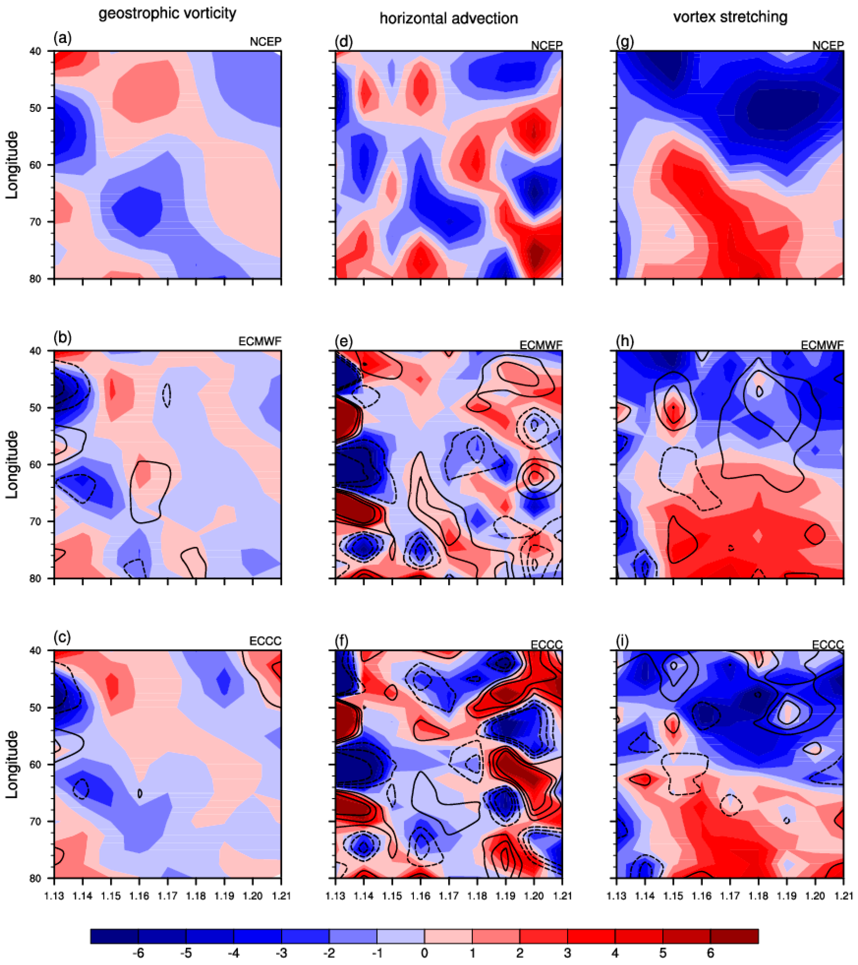
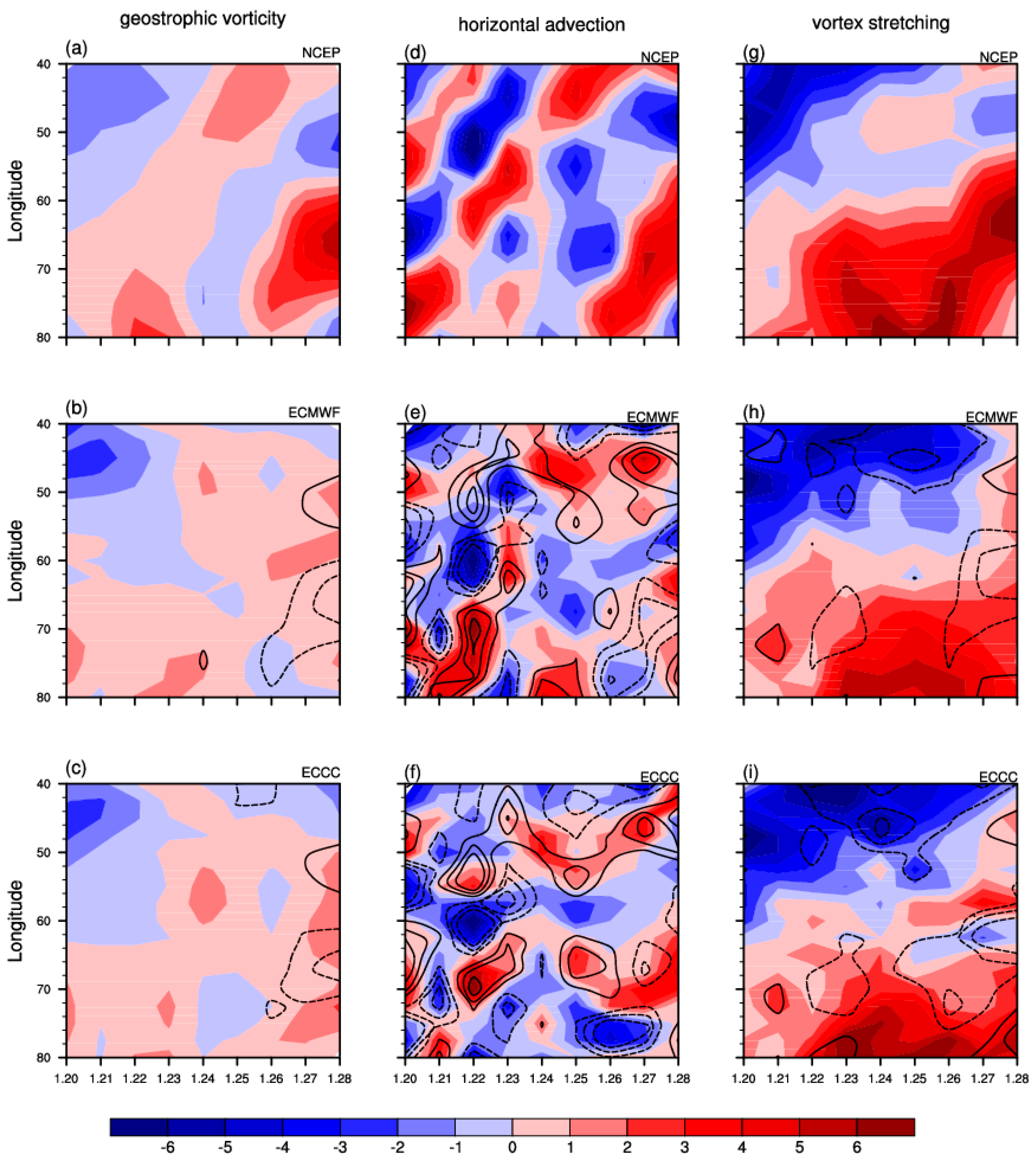
| geostrophic vorticity tendency | +0.35 * | +0.51* | +0.35 * | +0.51 * |
| horizontal vorticity advection | +0.09 | −0.02 | −0.01 | −0.12 |
| vortex stretching term | +0.71 * | +0.73 * | +0.81 * | +0.73 * |
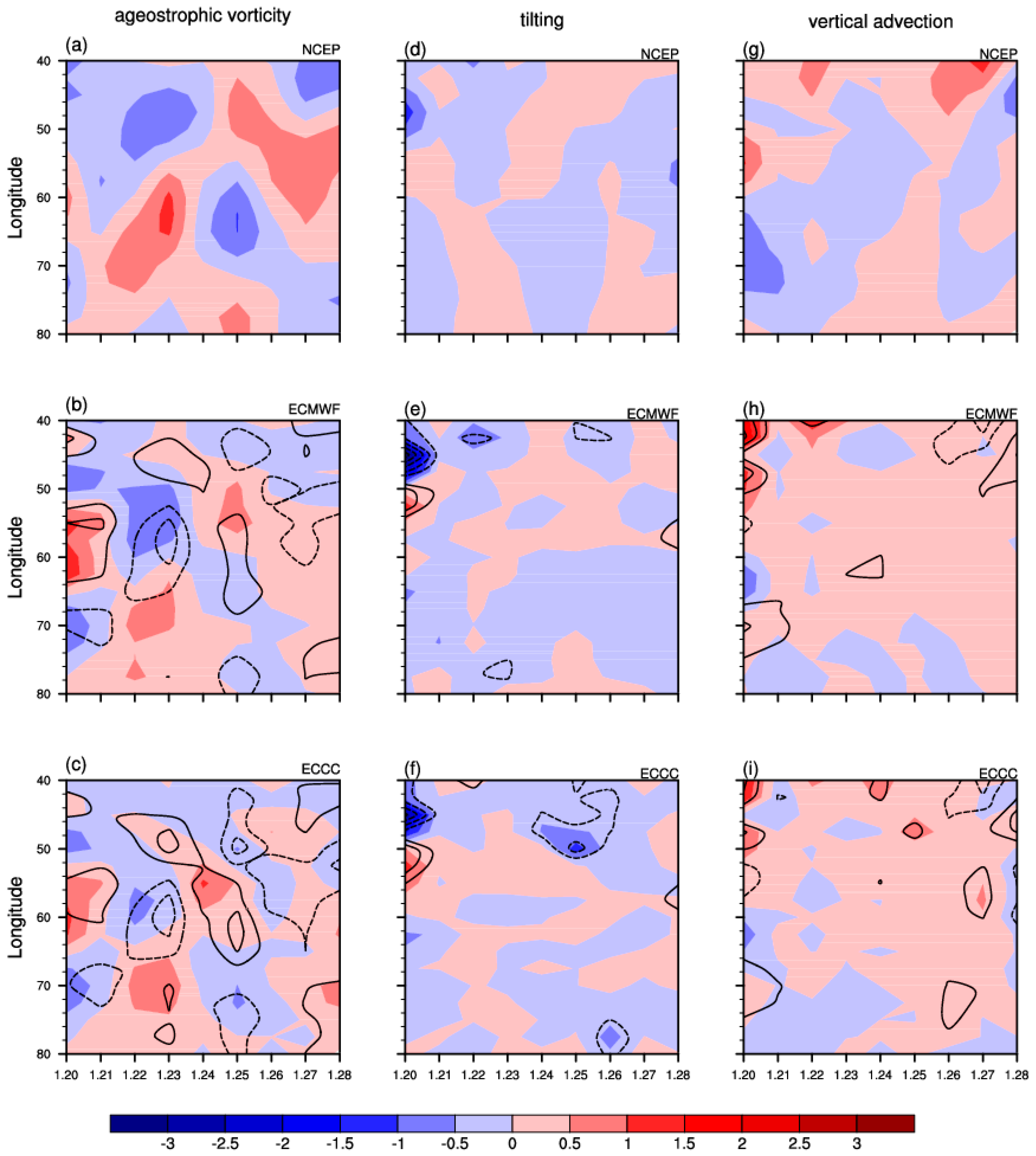
| tilting effect | +0.14 | +0.43 * | +0.42 * | +0.28 * |
| vertical vorticity advection | +0.24 * | +0.57 * | +0.32 * | +0.19 |
| ageostrophic vorticity tendency | +0.07 | +0.23 * | +0.40 * | +0.23 |
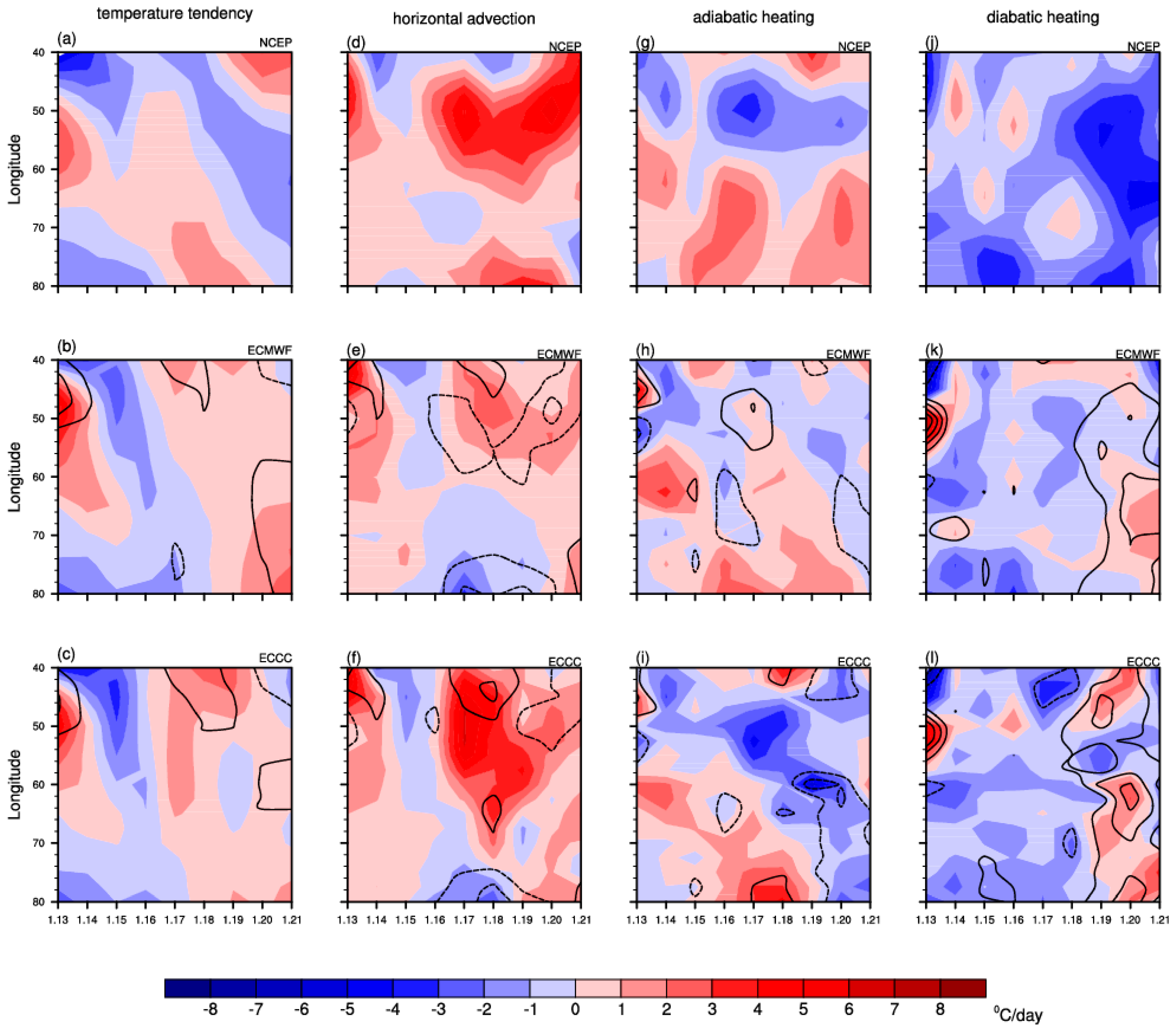
| temperature tendency | +0.30 | +0.46 * | +0.59 * | +0.46 * |
| horizontal temperature advection | +0.29 | +0.50 * | +0.70 * | +0.52 * |
| adiabatic heating | +0.22 | +0.37 * | +0.39 * | +0.23 |
| diabatic heating | +0.15 | +0.11 | +0.69 * | +0.65 * |
© 2020 by the authors. Licensee MDPI, Basel, Switzerland. This article is an open access article distributed under the terms and conditions of the Creative Commons Attribution (CC BY) license (http://creativecommons.org/licenses/by/4.0/).
Share and Cite
Chen, D.; Qiao, S.; Tang, S.; Cheung, H.N.; Liu, J.; Feng, G. Predictability of the Strong Ural blocking Event in January 2012 in the Subseasonal to Seasonal Models of Europe and Canada. Atmosphere 2020, 11, 538. https://doi.org/10.3390/atmos11050538
Chen D, Qiao S, Tang S, Cheung HN, Liu J, Feng G. Predictability of the Strong Ural blocking Event in January 2012 in the Subseasonal to Seasonal Models of Europe and Canada. Atmosphere. 2020; 11(5):538. https://doi.org/10.3390/atmos11050538
Chicago/Turabian StyleChen, Dong, Shaobo Qiao, Shankai Tang, Ho Nam Cheung, Jieyu Liu, and Guolin Feng. 2020. "Predictability of the Strong Ural blocking Event in January 2012 in the Subseasonal to Seasonal Models of Europe and Canada" Atmosphere 11, no. 5: 538. https://doi.org/10.3390/atmos11050538