Investigation and Optimization of Load Distribution for Tandem Cold Steel Strip Rolling Process

Abstract

In order to improve the cold rolled steel strip flatness, the load distribution of the tandem cold rolling process is subject to investigation and optimization. The strip deformation resistance model is corrected by an artificial neural network that is trained with the actual measured data of 4500 strip coils. Based on the model, a flatness prediction model of strip steel is established in a five-stand tandem cold rolling mill, and the precision of the flatness prediction model is verified by rolling experiment data. To analyze the effect of load distribution on flatness, the flatness of stand 4 is calculated to be 7.4 IU, 10.6 IU, and 16.8 IU under three typical load distribution modes. A genetic algorithm based on the excellent flatness is proposed to optimize the load distribution further. In the genetic algorithm, the classification of flatness of stand 4 calculated by the developed flatness prediction model is taken as the fitness function, with the optimal reduction of 28.6%, 34.6%, 27.3%, and 18.6% proposed for stands 1, 2, 3, and 4, respectively. The optimal solution is applied to a 1740 mm tandem cold rolling mill, which reduce the flatness classification from 10.8 IU to 3.2 IU for a 1-mm thick steel strip.

1. Introduction

Load distribution is the key to the cold rolling process, which is the critical factor for the yield and quality of steel strip products. In order to improve the production efficiency of a tandem cold rolling mill, the early work of load distribution optimization was mainly aimed at the power balance of each stand. Hu et al. [1] optimized the rolling schedule of aluminum hot tandem rolling to reduce energy consumption. A set-up optimization system was developed by Pires et al. [2], and the productivity of four stand tandem cold rolling mill was improved by the system. Reddy et al. [3] optimized the reduction schedule by distributing thickness in harmonic series for tandem cold rolling mill to maximize the throughput. With the development of the manufacturing industry, flatness accuracy becomes one of the most critical indicators of cold-rolled strip [4]. Constructing a reasonable load distribution schedule is the premise of obtaining good flatness quality.

To improve flatness quality, many scholars have done a large number of researches in load distribution optimization. Peng et al. [5] established the objective function of generalized shape and gauge decoupling load distribution optimization to improve the flatness control ability of each stand. Che et al. [6] proposed a multi-object optimization model in the process of tandem cold rolling based on an adaptive genetic algorithm. To determine the weight coefficient of each objective, Jia et al. [7] proposed a multi-objective differential evolutionary algorithm called MaximinDE to optimize load distribution. Li et al. [8] presented a multi-objective optimization model for load distribution for a hot strip mill based on the objective of rolling force ratio distribution to improve the strip flatness. Li et al. [9] proposed a differential evolution algorithm based on the evolutionary direction to optimized the rolling schedule for tandem cold rolling. The strip profile and rolling energy were selected as an objective function to improve flatness and power.

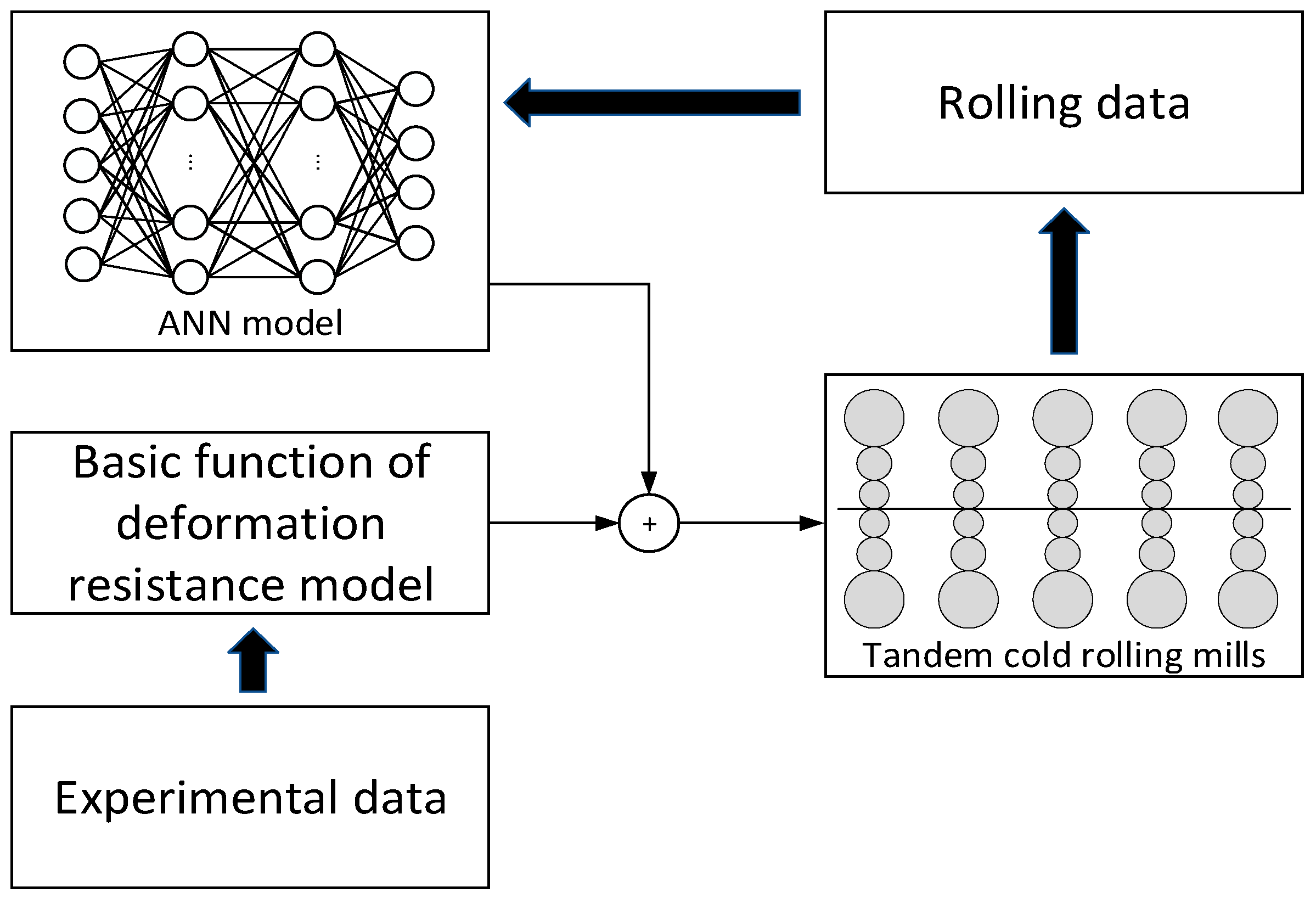
The critical point with load distribution optimization is that the determination of objective function with excellent flatness. Only a constant ratio crown is considered in the objective function in the above literature. If the hot strip has flatness defect, a constant ratio crown will inherit the flatness defect to the downstream stand. Besides, only the roll bending and rolling force are included in the function of a constant ratio crown, which is the inability to describe the complexity of the cold rolling process in detail. Hence, the objective function with excellent flatness can be further optimized. Moreover, the cold rolling process is complicated, and these optimization algorithms have no apparent physical meaning, cannot direct the further optimization of load distribution. In the present paper, to optimize the load distribution to improve the flatness quality, a high precision flatness prediction model is established. The flatness value calculated by the model is taken as the fitness function of genetic algorithm optimization to obtain an optimal load distribution of excellent flatness. Furthermore, the influence of load distribution on strip flatness is analyzed. Finally, the optimization results are applied to a 1740 mm tandem cold rolling mill, and the flatness quality is significantly improved. The technical routes of the present research are shown in Figure 1.

2. Modeling of Flatness Prediction for Tandem Cold Rolling

2.1. Modeling of Deformation Resistance of Cold-Rolled Steel

The deformation resistance model is the core of the rolling force and roll stack elastic deformation calculation, which is the premise of high precision calculation for flatness control.

Many studies have been performed around the deformation resistance model of the material to obtain precise rolling force and good flatness quality. Dzubinsky et al. [10] proposed a new equation for the prediction of hot rolling steel deformation resistance. This equation described the steel deformation behavior more accurately by using the data form the laboratory plastometer experiments. Lee et al. [11] investigated the work hardening behavior of ultrafine-grained twinning induced plasticity (TWIP) steel. The plastic deformation mechanism of ultrafine-grained TWIP steel was obtained based on the results from these experiments. Cai et al. [12] presented a dislocation-based model to study the strain-rate effect on the deformation resistance of metals and analyzed the influence of deformation on the resistance for dislocation generation. Eyckens et al. [13] experimentally observed the non-isotropic hardening in many steel materials and proposed a polycrystal plasticity model. The results showed that the non-isotropic hardening prediction was a significant improvement by the proposed model. The models established in the above literature were based on ideal laboratory conditions. Although these models are feasible in theory, their precision needs to be improved to express the complex hardening behavior of the cold rolling process. Therefore, it is necessary to establish the deformation resistance model by using a physical model to combine artificial neural network.

2.1.1. Basic Function of Deformation Resistance Model

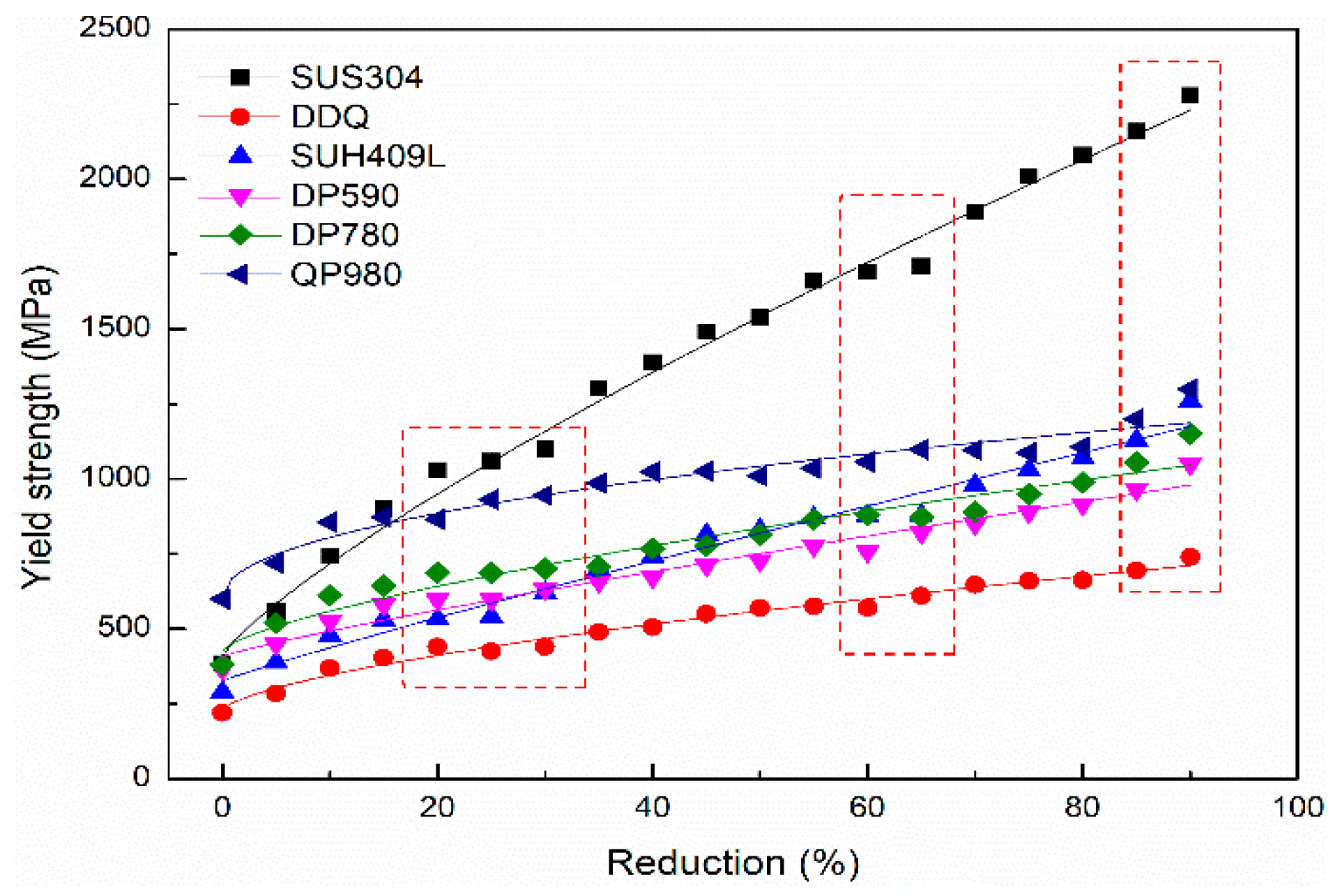
The basic function of the deformation resistance model was established by rolling and tensile experiments. The hot rolled plates were rolled to cold-rolled plates with different reduction by a four-high reversible cold mill in the laboratory. The reductions are from 5% to 85%, with an interval of 5%. Tensile tests were carried out on each reduction of cold-rolled plates, and the yield strength of different reductions was obtained.

The deformation resistance curve is related to the reduction and temperature, which could be expressed as Equation (1):

$$\sigma ={\sigma }_b·F_t$$

(1)

where ${\sigma }_b$ is the deformation resistance in ideal conditions and $F_t$ is the influence coefficient of temperature on deformation resistance of materials. ${\sigma }_b$ in Equation (1) can be expressed as Equation (2).

$${\sigma }_b={\sigma }_0+\left({\sigma }_1-{\sigma }_0\right)·{\epsilon }^m$$

(2)

where ${\sigma }_0$, ${\sigma }_1$, and m are the parameters that relate to the material and $\epsilon$ is the reduction. $F_t$ in Equation (1) as shown in Equation (3).

$$F_t=\frac{\frac{1}{2}-\frac{\arctan \left(t-t_0\right)}{\pi }}{\frac{1}{2}-\frac{\arctan \left(t_r-t_0\right)}{\pi }}$$

(3)

where t is the deformation temperature, t_r is the room temperature, and t₀ is the temperature in which the yield strength is half of that at room temperature.

The deformation resistance curves of typical steel grades are shown in Figure 2. As indicated in Figure 2, the fitting curves of deformation resistance deviate from the measured value when the reductions are 20%, 30%, 60%, and 90%.

2.1.2. Correction of Deformation Resistance by Artificial Neural Network

Different steel grades exhibit different work hardening characteristics. To make up the intrinsic imperfection of the basic function of the deformation resistance model, four reduction points (20%, 30%, 60%, 90%) of the deformation resistance curve are corrected by an artificial neural network (ANN) established based on the actual measured industrial data. The corrected deformation resistance model ${\sigma }_F$ as shown in Equation (4).

$${\sigma }_F=\sigma ·C$$

(4)

where the C is the correction factor of the deformation resistance model as follows:

$$C=\frac{{\displaystyle \sum _{l=1}^n{W}_l}{F}_l}{{\displaystyle \sum _{l=1}^n{W}_l}}$$

(5)

where n is the number of correction points (n = 4). F_l is the correction factor of reduction. W_l is the influence factor of correction points. l is the serial number of correction points (l = 1, 2, 3, 4).

The influence of the correction points on the deformation resistance curve obeys the Gaussian distribution, as shown in Equation (6).

$$W_l={\exp }^{-\frac{{\epsilon }_e-{\epsilon }_l}{{\eta }^2}}$$

(6)

where ${\epsilon }_e$ is the reduction of the deformation resistance curve, ${\epsilon }_l$ is the reduction of the correction points, and $\eta$ is the standard deviation.

Back propagation algorithm artificial neural network (BP-ANN) was proposed by Rumelhart et al. [14], and widely used in flatness recognition (Peng et al. [15]) and parameter prediction (Wang et al. [16]) of the cold rolling process. BP-ANN is trained according to the error back propagation algorithm, and the weights of BP-ANN are modified until meeting the requirements of the accuracy. The learning procedures of BP-ANN are as follows:

Step 1: Set the initial weights and thresholds of the network.

Step 2: Determine the input mode, output mode and training mode of the network.

Step 3: Input a sample data to the network, calculate the output of the network layer by layer and compare the output result with the expected value.

Step 4: Calculate the total error of the output node, and propagate these errors back to the network using a back propagation algorithm to calculate the gradient. Using gradient descent algorithm to adjust the weight of the network to reduce the error of the output layer.

Step 5: Input the sample into the network again, and repeat Step 3 and Step 4 until the network meets the accuracy requirements.

In Equation (5), F_l is determined by a classical BP-ANN, which was trained with the actual measured industrial data. A dataset of 4500 coils has been gathered by a 1740mm tandem cold rolling mill. The data of 4000 coils were used to train, and the other 500 coils were used to predict the F₁, F₂, F₃ and F₄. The number of hidden layers is 2. The number of nodes in hidden layer1 and hidden layer2 are 12 and 8, respectively. The inputs of ANN are the chemical composition of steel, rolling temperature, the thickness of the hot strip, and the thickness of the entrance and exit. The outputs are the correction factor F₁, F₂, F₃ and F₄. The flow chart of the deformation resistance model corrected by ANN, as shown in Figure 3.

The deformation rate of material will increase with the increase of rolling speed, which will affect the deformation resistance. The deformation rate of each stand can be calculated according to the Ekelend formula [3]:

$${\stackrel{\cdot }{\epsilon }}_k=\frac{1000}{60}·\frac{2v_k}{2-s{r}_k}\sqrt{\frac{s{r}_k}{h_{k-1}·R_k^{\prime }}}$$

(7)

Where k is the stand number. ${\stackrel{\cdot }{\epsilon }}_k$ is the deformation rate of stand k. v_k is the rolling speed of stand k. $R_k^{\prime }$ is work roll flattening radius of stand k.

The deformation resistance affected by the rolling speed is calculated as follows:

$${\sigma }_{dk}={\sigma }_{Fk}·{\left(1000·\stackrel{\cdot }{{\epsilon }_k}\right)}^{\alpha }$$

(8)

where σ_dk is the deformation resistance of stand k affected by the rolling speed, σ_Fk is the deformation resistance of stand k corrected by ANN, and α is the strain rate sensitivity coefficient.

2.1.3. Evaluation of Proposed Deformation Resistance Model

In order to evaluate the proposed deformation resistance model, the deformation resistance model corrected by ANN of DP780 steel was established. The results of W_lF_l and C are indicated in Figure 4a. The deformation resistance curve corrected by the ANN is shown in Figure 4b. Compared with the traditional model, the correction model described the work hardening characteristics of cold-rolled steel in more detail.

2.2. Modeling of Rolls Elastic Deformation

The profile of the final product is directly affected by rolls elastic deformation. In order to obtain a better simulation of elastic deformation of rolls in the actual rolling process, the finite element method (FEM) is widely used in the establishment of elastic deformation of rolls. Linghu et al. [17] developed a model for cold rolling mill based on a three-dimensional (3D) FEM to investigating the flatness control capability. Wang et al. [18] analyzed the rigidity characteristics of UCM cold rolling mill on account of intermediate roll shifting by a 3D elastic-plastic FEM. Meanwhile, Wang et al. [19] analyzed the flatness actuator efficiencies for universal crown mill (UCM) cold rolling mill based on 3D elastic-plastic FEM to improving the accuracy of flatness control. Nonetheless, the FEM method needs a long calculation time and have a convergence problem, which is not suitable for an online control process of the cold rolling flatness. In this section, the rolls elastic deformation model is established based on the influence function method.

The contour of rolls is needed before calculating the rolls elastic deformation. The thermal contour $C_t$ and wear contour $C_w$ are calculated as Equations (9) and (10), respectively.

$$C_t=2\left(1+\nu \right)\frac{{\beta }_t}{R}{\displaystyle {\int }_0^R\left(T\left(r,z\right)-T_0\left(r,z\right)\right)}rdr$$

(9)

where $\nu$ is the Poisson’s ratio of rolls, ${\beta }_t$ is the coefficient of thermal expansion of rolls, $R$ is the radius of work rolls, $r$ and $z$ are the coordinates of the roll, $T_0\left(r,z\right)$ is the initial temperature, and $T\left(r,z\right)$ is the real-time temperature.

$$C_w=\frac{L}{\pi 2R}\left\{q\left(y\right)\left[g_r+k_r\left|1-\frac{R_W\left(i\right)}{R_I\left(i\right)}·\frac{R_{10}}{R_{20}}\right|\right]+q\prime \left(y\right)g_s\right\}$$

(10)

where $q\left(y\right)$ is the pressure between work roll and intermediate roll. $q\prime \left(y\right)$ is rolling force, $g_r$ and $g_s$ are the rolling wear coefficient between rolls and between roll and strip, respectively. $k_r$ is the slide wear coefficient between roll and strip. $R_W\left(i\right)$ and $R_I\left(i\right)$ are the loaded radius of work roll and intermediate roll, respectively. $R_{10}$ is the working radius of work roll and $R_{20}$ is the working radius of intermediate roll.

To establish the rolls elastic deformation model by influence function method, the rolls and the load on rolls should be discrete, as shown in Figure 5.

The load of each unit is obtained by rolling force distribution. The total deformation of unit i is calculated as shown in Equation (11).

$$y\left(i\right)={\displaystyle \sum _{j=1}^{n}g\left(i,j\right)}p\left(j\right)i=1\sim n$$

(11)

where $y\left(i\right)$ is the total deformation of unit i th, $y\left(i\right)$ can be used to represent both the deflection and the flattening of rolls. $g\left(i,j\right)$ is the influence function. $p\left(j\right)$ is unit force that is identified by the strength of strip and the profile of entry and exit.

The deflection of rolls is calculated according to Equations (12) and (13).

$$Y_W{=\mathrm{G}}_{\mathrm{W}}\left(Q_{WI}-P\right)-G_{FW}{F}_W$$

(12)

$$Y_I{=\mathrm{G}}_{\mathrm{I}}\left(Q_{IB}-Q_{WI}\right)-G_{FI}{F}_I$$

(13)

where Y_W and Y_I are the deflection of work roll and intermediate roll, respectively. Q_WI is the contact stress between work roll and intermediate roll, and Q_IB is the contact stress between intermediate roll and backup roll. G_W and G_I are the deflection influence function of work roll and intermediate roll, respectively. F_W is the work roll bending force and F_I is the intermediate roll bending force. P is the rolling force.

The flattening of rolls is shown in Equations (14) and (15).

$$Y_{WS}{=\mathrm{G}}_{\mathrm{WS}}P$$

(14)

$$Y_{WI}{=\mathrm{G}}_{\mathrm{WI}}{Q}_{WI}$$

(15)

where Y_WS is the flattening of work caused by rolling force. Y_WI is the flattening between work roll and intermediate roll.

Therefore, the profile of roll gap can be obtained, and then, the strip transverse thickness distribution after rolling is calculated in Equation (16).

$$h\left(i\right)=h_0+\left(Y_{ws}\left(i\right)-Y_{ws0}\right)+\left(M_w\left(i\right)-Y_w\left(i\right)\right)$$

(16)

where h(i) is the vector of strip transverse thickness distribution after rolling, h₀ is the half thickness of the center point of the strip. Y_ws (i) is the vector of flattening of work roll caused by rolling force. Y_ws0 is the flattening value of the center point of work roll caused by rolling force. M_w (i) is the vector of crown of the work roll. Y_w (i) is the vector of the defection value of work roll. The flow diagram of the elastic deformation calculation of the roll stack is shown in Figure 6.

The iterative corrections of the calculated value of pressure, thickness profile and tension distribution are carried out by the exponential smoothing in Equation (17).

$$y_I^n=y_I^{n-1}+\lambda \left[y_C^n-y_I^{n-1}\right]$$

(17)

where $y_I^n$ is the nth iteration value of pressure, thickness profile, and tension distribution. $y_I^{n-1}$ is the n-1th iteration value of pressure, thickness profile and tension distribution. $y_C^n$ is the nth calculated value of pressure, thickness profile and tension distribution. $\lambda$ is the constant value of smooth.

2.3. Modeling of Residual Stress of Strip after Rolling

To obtain the flatness of strip after rolling, the model of the residual stress of strip after rolling must be established by the transverse thickness distribution of the strip before and after rolling. When the compressive residual stress exists on the strip, the residual stress is negative and the flatness defect appears. According to the volume constancy, the following Equation (18) can be obtained.

$$\frac{\Delta l(i)}{l}=\frac{\Delta L(i)}{L}+\frac{\Delta H(i)}{H}-\frac{\Delta h(i)}{h}-\Delta b(i)$$

(18)

where $\Delta l(i)$ is the variation of length after rolling. $\Delta L(i)$ is the variation of length before rolling. $\Delta h(i)$ is the variation of thickness after rolling. $\Delta H(i)$ is the variation of thickness before rolling. $\Delta b(i)$ is the variation of width after rolling. $l$ is the average length after rolling. L is the average length before rolling. $h$ is the average thickness after rolling. $H$ is the average thickness before rolling.

According to Equation (8), the residual stress of ith is shown in Equation (19).

$$\Delta \sigma (i)=-\frac{E}{1-{\nu }^2}\frac{\Delta l(i)}{l}=\frac{E}{1-{\nu }^2}\left[\frac{\Delta h(i)}{h}-\frac{\Delta L(i)}{L}-\frac{\Delta H(i)}{H}+\Delta b(i)\right]$$

(19)

where $\nu$ is the Poisson’s ratio, Equation (19) can be rewritten as shown in Equation (20).

$$\Delta \sigma (i)=\frac{E}{1-{\nu }^2}\left[1+\frac{h(i)}{h}-\frac{L(i)}{L}-\frac{H(i)}{H}+\Delta b(i)\right]$$

(20)

where $\Delta b(i)$ can be calculated per Equation (21) according to the stream surface strip element method [21].

$$\Delta b(i)=\mu (i+1)-\mu (i)$$

(21)

where μ(i) is the lateral displacement of metal. μ(i) can be calculated as follows:

$$\mu \left(i\right)=\frac{\Delta BshKx\left(i\right)}{2shM}+\frac{a_{2}B}{M^2}\left(\frac{2x\left(i\right)}{B}-\frac{shKx\left(i\right)}{shM}\right)+\frac{2a_{4}B}{M^2}\times \left[{\left(\frac{2x\left(i\right)}{B}\right)}^3+\frac{6}{M^2}\left(\frac{2x\left(i\right)}{B}\right)-\left(1+\frac{6}{M^2}\right)\frac{shKx\left(i\right)}{shM}\right]$$

(22)

where

$$\begin{array}{l}M=\sqrt{\frac{4{\eta }_1}{{\eta }_2+3}}, {\eta }_1=\frac{4\mu \overline{P}{B}^2}{1.15·lc·{\sigma }_F·\left(H+h\right)}, {\eta }_1=\frac{8E_s}{1.15·{\sigma }_F·\left(1-{\nu }^2\right)}\left(\frac{H-h}{H+h}\right), a_2=\frac{{\eta }_2}{{\eta }_2+3}\left(\frac{b_2}{H}-\frac{B_2}{h}\right), \\ a_4=\frac{{\eta }_2}{{\eta }_2+3}\left(\frac{b_4}{h}-\frac{B_4}{H}\right)\end{array}$$

(23)

where ΔB is the total spread of the strip. K is the shear deformation resistance of the strip. x(i) is the transverse coordinate of the strip unit. lc is the contact length. $\overline{P}$ is the average rolling force. μ is the friction coefficient. B₂ and B₄ are the thickness distribution fitting coefficient of entry strip. b₂, b₄ are the thickness distribution fitting coefficient of exit strip. B₂, B₄, b₂, and b₄ are fitted as follows:

$$\{\begin{array}{l}H\left(i\right)=B_0+B_2{\left(\frac{2x\left(i\right)}{B}\right)}^2+B_4{\left(\frac{2x\left(i\right)}{B}\right)}^4\\ h\left(i\right)=b_0+b_2{\left(\frac{2x\left(i\right)}{B}\right)}^2+b_4{\left(\frac{2x\left(i\right)}{B}\right)}^4\end{array}$$

(24)

The relationship between residual stress and flatness can be described in Equation (25).

$$flatness(i)=-\frac{\Delta \sigma (i)}{E_s}$$

(25)

where flatness(i) is the flatness value of each transverse unit, $\Delta \sigma$ is the residual stress of the strip, and E_s is the elastic modulus of the strip.

2.4. Verification of the Flatness Prediction Model

The flatness prediction model is verified in a tandem cold rolling mill, by comparing the rolling force and flatness of the cold-rolled strip between the calculated results and measured values. The steel samples are SUH409L, DP590, DP780 and QP980. The parameters for calculation are obtained from Primary Data Input (PDI). The verification results are shown in Figure 7. As indicated in Figure 7a, the relative error of the rolling force of steel samples between simulation and measurement is less than 5%. Meanwhile, the maximum absolute error of the flatness is less than 10 IU, as shown in Figure 7b–e.

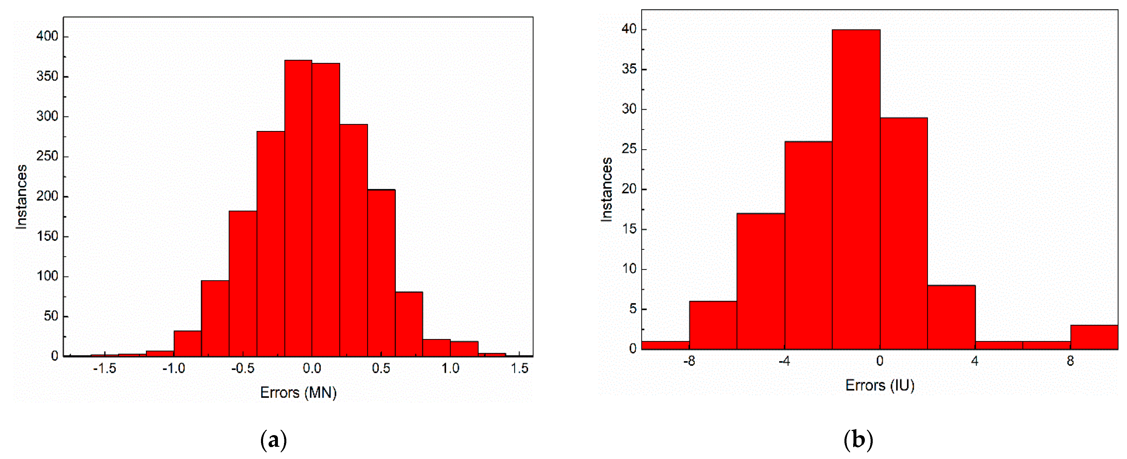
The error distribution histogram of rolling force and strip flatness are shown in Figure 8. As indicated in Figure 8, the overall error is approximately symmetrical normal distribution, and the error distribution histogram is stable. To evaluate the flatness prediction model more quantitatively, the correlation coefficient, mean absolute error, mean absolute percentage error, standard deviation and maximum absolute error are calculated, and the results are shown in

Table 1. The error indexes of rolling force and strip flatness.

Error Index Type	Rolling Force	Strip Flatness
Correlation coefficient (R)	0.9242	0.9278
Mean absolute error (MAE)	0.3269	2.5227
Mean absolute percentage error (MAPE, %)	1.9179	-
Standard deviation (SD)	0.2504	2.1944
Maximum absolute error	1.6031	9.1346

. As shown in Table 1, the correlation coefficient of rolling force and strip flatness are 0.9242 and 0.9278, respectively. The mean absolute error of rolling force and strip flatness are 0.3269 MN and 2.5227 IU, respectively. The standard deviation of rolling force and strip flatness are 0.2504 MN and 2.1944 IU, respectively. The maximum absolute error of rolling force and strip flatness are 1.6031 MN and 9.1346 IU, respectively. Due to the measured value of strip flatness exists zero value, the mean absolute percentage error is unsuitable for evaluate the accuracy of flatness calculation, the mean absolute percentage error of strip flatness is not calculated. As shown in Figure 7 and Figure 8 and Table 1, the developed model has a high accuracy and can be used as an effective tool to investigate the relationship between load distribution and strip flatness.

3. Influence of Load Distribution on Flatness

To reveal the influence of load distribution on strip flatness, the simulations are done based on parameters of a 1740 mm 5-stand tandem cold mill. Stand 1, stand 2, stand 3, stand 4, and stand 5 are denoted by S1, S2, S3, S4, and S5. The rolling parameters for simulation are shown in

Table 2. The rolling parameters for the simulation.

Name	Value
Work roll diameter/length (mm)	425/1740
Intermediate roll diameter/length (mm)	490/1990
Backup roll diameter/length (mm)	1300/1750
Strip width (mm)	1250
Entry and exit thickness of the strip (mm)	3.5/1
Material	DP780

. The material for simulation is DP780 steel.

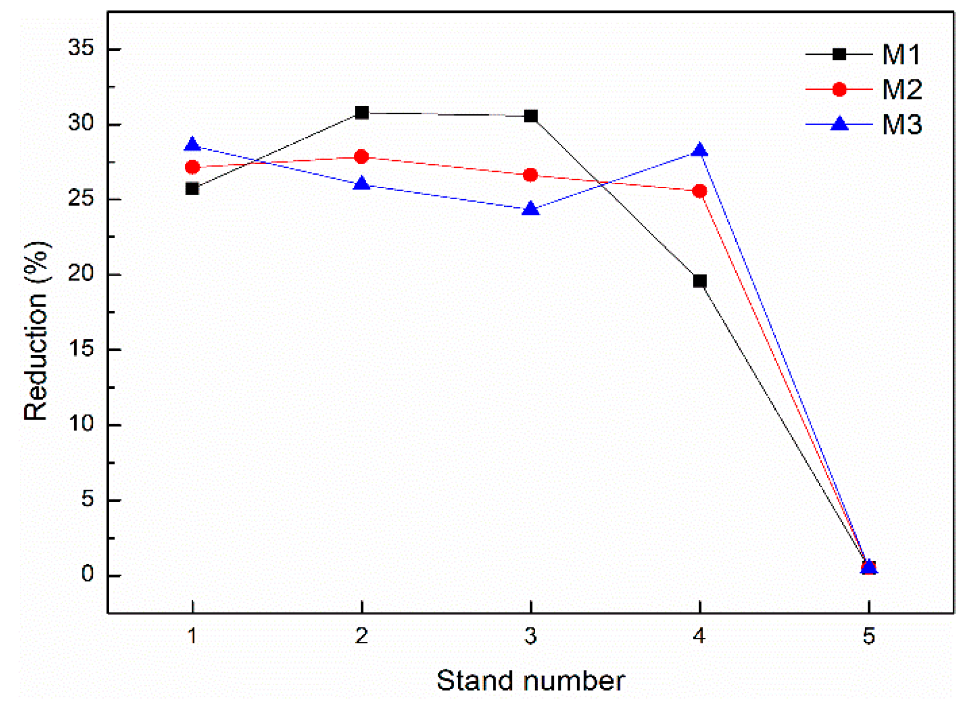
To analyze the effect of load distribution on strip flatness, the load distribution is set to three modes, which are denoted by M1, M2 and M3, respectively. The reduction of S5 for M1, M2 and M3 are the same (0.5%) due to the constant rolling force. M1, M2, and M3 are the typical load distribution modes determined by manual experience in a 1740 mm tandem cold rolling mill. The reduction of each stand in M1, M2, and M3 are shown in

Table 3. The reduction of each stand under different load distribution mode.

Mode	Reduction %
	S1	S2	S3	S4	S5
M1	25.7	30.8	30.6	19.6	0.5
M2	27.1	27.8	26.6	25.6	0.5
M3	28.1	26.0	24.3	28.2	0.5

and Figure 9. As shown in Figure 9, the reduction of S4 is lower than S1, S2, and S3 in M1. Conversely, the reduction of S4 is higher than S1, S2, and S3 in M3. The reduction of each stand is equal in M2. The roll bending force is set to a median value (300 kN) while the load distribution is studied. S4 is the last stand without flatness feedback control. The flatness adjustment range is limited by the equipment capacity in S5. Therefore, the flatness of S4 has a significant effect on the flatness of the finished strip. Hence, the present research focuses on the flatness simulation of S4. The classification of strip flatness is calculated according to Equation (26).

$$C_f=\frac{{\displaystyle \sum _{i=1}^n\left|flatnes{s}_i\right|}}{n}$$

(26)

where C_f is the classification of strip flatness, n is the number of strip transverse units.

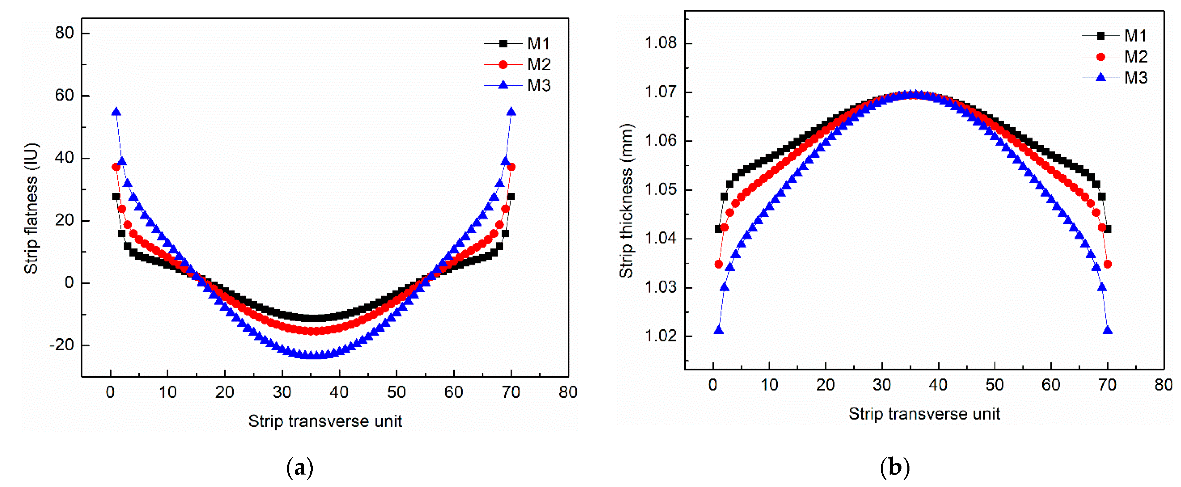
The computation of flatness of S4 under different load distribution are shown in Figure 10a. The C_f of S4 under M1, M2 and M3 are 7.4 IU, 10.6IU, and 16.8 IU, respectively. The flatness of M1 is better than the other two modes, and the flatness of M3 presents a defect of edge wave. The thickness profile of S4 under different load distributions are shown in Figure 10b. The crown of the strip after rolling increases with the increase of the reduction of S4.

The profile of the roll gap during the cold rolling process can be described as the Equation (27).

$$CR=\frac{P}{K_P}+\frac{F}{K_F}+W_C$$

(27)

where CR is the crown of the roll gap, P is the rolling force, and F is the roll bending force, K_P and K_F are the transverse rigidity of rolling force and bending force, respectively, and W_C is the roll profile.

The higher reduction induces the higher rolling force. According to the Equation (27), to keep the excellent flatness, when the rolling force increases, the bending force must increase to ensure the crown of the roll gap unchanged. The strip crown of S4 under different load distribution are simulated to analyze the relationship between reduction and roll bending capacity. The work roll bending force is set to 100, 200, and 300 kN in each model of load distribution. The changing trend of strip crown under different load distributions is shown in Figure 11. The strip crown decreases from 0.155 mm to 0.0548 mm with the work roll bending force increasing from 100 kN to 300 kN in M1, the variation of the strip is 0.1002 mm. The changes of the strip are 0.084 mm and 0.076 mm in M2 and M3, respectively. The capacity of roll bending to control flatness decreases as the increase of reduction.

4. Optimization of Load Distribution by Genetic Algorithm

As indicated in Section 3, the classification of strip flatness is improved by decreasing the reduction of S4. The reduction of S1–S3 will increase with the decrease of the reduction of S4, which may induce the flatness defect. Hence, the reduction of S4 cannot be an unlimited decrease. Genetic algorithm (GA) is a global optimization calculation method which born in the 1960s. GA has been successfully applied in searching the optimal solution of parameters of the rolling process (Son et al. [22], Kadkhodaei et al. [23] and Cao et al. [24]). GA is a random search algorithm which uses the goal of biological evolution, and the calculation procedures are as follows:

Step 1: Set a set of random initial solutions.

Step 2: Calculate the fitness of all individuals in the population and evaluate the fitness.

Step 3: Determine whether the current solution meets the optimization goal, or whether the genetic generation meets the requirements. If so, go to Step 6.

Step 4: Select a partial solution from the current solution to enter the genetic operation according to the fitness evaluation of Step 2.

Step 5: Perform genetic operation (crossover, mutation) on the selected solutions to generate a new set of solutions, and go to Step 2.

Step 6: Output the current solution.

To determine the optimal load distribution under the condition of good flatness, the load distribution is further optimized based on the genetic algorithm with excellent flatness.

4.1. Fitness Function

The fitness is defined as follows:

$$Fitness=\frac{1}{C_{f4}}$$

(28)

where the C_f4 is the classification of strip flatness of S4 calculated by Equation (26).

4.2. Constraint Conditions

The rolling force, rolling torque, and rolling power cannot exceed the limit of equipment, and the constraints are defined as follows:

$$\{\begin{array}{l}R{F}_i\le R{F}_{i,\max }\\ P_i\le P_{i,\max }\\ T_i\le T_{i,\max }\end{array}$$

(29)

where $R{F}_i$ is the rolling force of stand i, $R{F}_{i,\max }$ is the maximum rolling force of stand i. $P_{i,\max }$ is the maximum rolling power of stand i. $T_i$ and $T_{i,\max }$ are the rolling torque and the maximum rolling torque of stand i, respectively.

The lower and upper reduction limits of S1–S4 are 10% and 40%, respectively.

4.3. Load Distribution Optimization Procedure

The steps of load distribution optimization are as follows:

Step 1: Randomly generate a set of reductions that meet the constraints.

Step 2: The C_f4 is calculated by the flatness prediction model, as established in Section 2.

Step 3: Chromosome evaluation is carried out according to the C_f4, and the optimal individual is selected for the genetic operation.

Step 4: Start the genetic calculation. After the selection, crossover and variation operation, the flatness prediction model is called to calculate the C_f4. The chromosome is re-evaluated, and the optimal individual is preserved.

Step 5: The optimal load distribution is output if the number of iterations satisfies the evolutionary generation. Otherwise, return to Step 2.

The optimization flow chart is shown in Figure 12.

4.4. Optimization Results

The optimization is based on the parameters of a 1740 mm tandem cold rolling mill in Section 3. The work roll bending force and intermediate roll bending force are set to a median value (300 kN). According to the previous work of GA for load distribution [7,8], the size of the genetic population is 100, the crossover probability is 0.9, and the mutation probability is 0.1. The best fitness evolution for the genetic algorithm is shown in Figure 13a, and the reduction of S1–S4 evolution is shown in Figure 13b.

As indicated in Figure 13a, the solution process is converged after 30 generations. As shown in Figure 13b, the reduction of S1 and S3 increased slightly. The reduction of S2 increased from 23.8% to 31%, while the reduction of S4 decreased from 24.3% to 18.5%. The optimization results are consistent with the simulation results in the trend of Section 3. The optimal reduction of 28.6%, 34.6%, 27.3%, and 18.6% is proposed for S1, S2, S3, and S4, respectively.

5. Industrial Application

The optimization results are applied to a 1740 mm tandem cold mill, and the flatness meter was equipped behind the finish stand for the strip flatness measurement. The material for industrial application was formed with DP780 steel. The thickness of the hot strip was 3.5 mm, and the width was 1250 mm. The exit thickness was 1.0 mm.

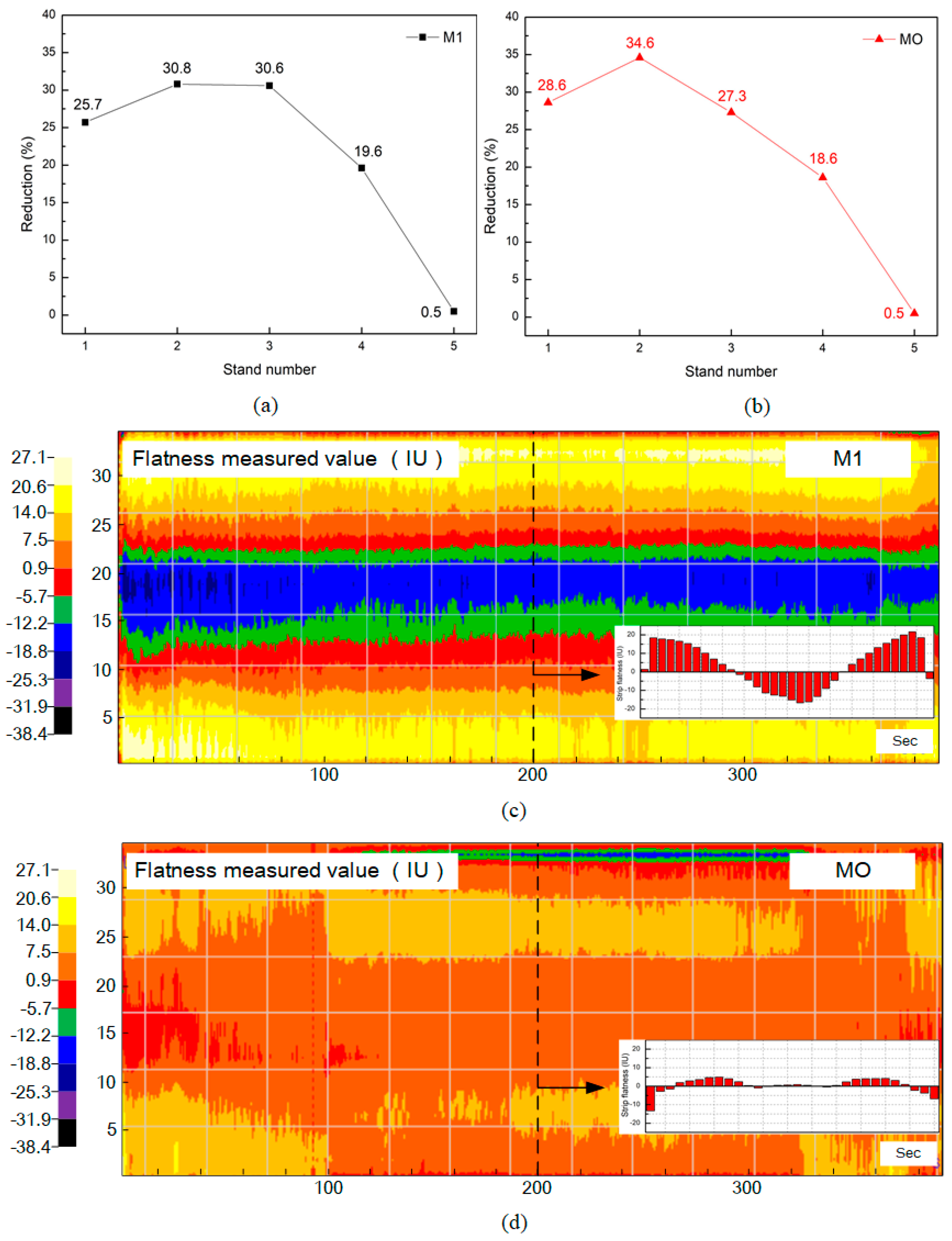
To verify the simulation and optimization results of the effect of load distribution on flatness in Section 3, two load distribution modes were carried out in industrial experiments. M1 is the load distribution mode of Section 3 and MO is the optimized scheme based on the optimization results in Section 4. The reduction of M1 and MO are shown in Figure 14a,b. As shown in Figure 14a,b, the reduction of S3 and S4 in M1 was higher than MO. The flatness under M1 and MO were compared and the actual measured values are shown in Figure 14c,d.

As shown in Figure 14c, the whole strip coil under M1 had a serious edge wave defect. The C_f was 10.8 IU calculated by Equation (26), and the local flatness in the edge exceeded 20 IU. Figure 14d indicated the actual measured values of flatness under MO, the flatness quality of the whole strip coil were improved compared with M1. The C_f was 3.2 IU calculated by Equation (26), and the maximum local flatness was less than 5 IU.

6. Conclusions

1. A deformation resistance model of strip steel was established and verified based on the correction of an artificial neural network, which described the work hardening characteristics of cold-rolled strip steel in more detail.

2. A flatness prediction model was established and verified based on the corrected deformation resistance model and the influence function method. The relative error of the rolling force calculated by the model is less than 5%, and the absolute error of flatness is within 10 IU. The provided flatness prediction model has an acceptable accuracy to meet the requirements of the present study.

3. The influence of load distribution on flatness was analyzed based on the established flatness prediction model. The load distribution is set to three typical modes, which were denoted by M1, M2, and M3, respectively. The reduction of M1 for S1, S2, S3, and S4 are 25.7%, 30.8%, 30.6%, and 19.6%. The reduction of M2 for S1, S2, S3, and S4 are 27.1%, 27.8%, 26.6%, and 25.6%. The reduction of M3 for S1 S2, S3, and S4 are 28.1%, 26.0%, 24.3%, and 28.2%. The Cf4 under M1, M2, and M3 were 7.4 IU, 10.6 IU, and 16.8 IU, respectively.

4. In order to improve the cold-rolled strip flatness, the genetic algorithm was used to optimize the load distribution. The Cf4 calculated by the established flatness prediction model was taken as the fitness function, and the optimal distribution mode (MO) was obtained. The reduction of 28.6%, 34.6%, 27.3%, and 18.6% was proposed for S1, S2, S3, and S4, respectively. The optimization results were applied to a 1740-mm tandem cold rolling mill, and the strip flatness was reduced from 10.8 IU to 3.2 IU for a 1-mm thick steel strip.

References

- Hu, Z.; Yang, J.; Zhao, Z.; Sun, H.; Che, H. Multi-objective optimization of rolling schedules on aluminum hot tandem rolling. Int. J. Adv. Manuf. Technol. 2016, 85, 85–97. [Google Scholar] [CrossRef]
- Pires, C.; Ferreira, H.; Sales, R.; Silva, M. Set-up optimization for tandem cold mills: A case study. J. Mater. Process. Technol. 2006, 173, 368–375. [Google Scholar] [CrossRef]
- Reddy, N.; Suryanarayana, G. A set-up model for tandem cold rolling mills. J. Mater. Process. Technol. 2001, 116, 269–277. [Google Scholar] [CrossRef]
- Cao, J.; Chai, X.; Li, Y.; Kong, N.; Jia, S.; Zeng, W. Integrated design of roll contours for strip edge drop and crown control in tandem cold rolling mills. J. Mater. Process. Technol. 2018, 252, 432–439. [Google Scholar] [CrossRef]
- Peng, P.; Yang, Q. Generalized shape and gauge decoupling load distribution optimization based on IGA for tandem cold mill. J. Iron Steel Res. Int. 2009, 16, 30–34. [Google Scholar] [CrossRef]
- Che, H.; Han, X.; Yang, J.; Li, L. Optimization of Schedule with Multi-Objective for Tandem Cold Rolling Mill Based on IAGA. In Proceedings of the 2010 International Conference on Mechanic Automation and Control Engineering, Wuhan, China, 26–28 June 2010. [Google Scholar]
- Jia, S.; Li, W.; Liu, X.; Du, B. Multi-objective load distribution optimization for hot strip mills. J. Iron Steel Res. Int. 2013, 20, 27–32. [Google Scholar] [CrossRef]
- Li, W.; Liu, X.; Guo, Z. Multi-objective optimization for draft scheduling of hot strip mill. J. Cent. South. Univ. 2012, 19, 3069–3078. [Google Scholar] [CrossRef]
- Li, Y.; Fang, L. Robust multi-objective optimization of rolling schedule for tandem cold rolling based on evolutionary direction differential evolution algorithm. J. Iron Steel Res. Int. 2017, 24, 795–802. [Google Scholar] [CrossRef]
- Dzubinsky, M.; Kovac, F.; Petercakova, A. New form of equation for deformation resistance prediction under hot rolling industrial conditions. Scri. Mater. 2002, 47, 119–124. [Google Scholar] [CrossRef] [Green Version]
- Lee, S.; Lee, S.J.; Cooman, D.B.C. Work hardening behavior of ultrafine-grained Mn transformation-induced plasticity steel. Acta Mater. 2011, 59, 7546–7553. [Google Scholar] [CrossRef]
- Cai, M.; Shi, H.; Yu, T. A dislocation-based constitutive description of strain-rate effect on the deformation resistance of metals. J. Mater. Sci. 2011, 46, 1087–1094. [Google Scholar] [CrossRef]
- Eyckens, P.; Mulder, H.; Gawad, J.; Vegter, H.; Roose, D.; Van den Boogaard, T.; Van Beal, A.; Van Houtte, P. The prediction of differential hardening behaviour of steels by multi-scale crystal plasticity modelling. Int. J. Plast. 2015, 73, 119–141. [Google Scholar] [CrossRef] [Green Version]
- Rumelhart, D.; Hinton, G.; Williams, R. Learning representations by back-propagating errors. Nature 1986, 323, 533–536. [Google Scholar] [CrossRef]
- Peng, Y.; Liu, H.; Du, R. A neural network-based shape control system for cold rolling operations. J. Mater. Process. Technol. 2008, 202, 54–60. [Google Scholar] [CrossRef]
- Wang, Z.; Gong, D.; Li, X.; Li, G.; Zhang, D. Prediction of bending force in the hot strip rolling process using artificial neural network and genetic algorithm (ANN-GN). Int. J. Adv. Manuf. Technol. 2017, 93, 3325–3338. [Google Scholar] [CrossRef]
- Linghu, K.; Jiang, Z.; Zhao, J.; Li, F.; Wei, D.; Xu, J.; Zhang, X.; Zhao, X. 3D FEM analysis of strip shape during multi-pass rolling in a 6-high CVC cold rolling mill. Int. J. Adv. Manuf. Technol. 2014, 74, 1733–1745. [Google Scholar] [CrossRef] [Green Version]
- Wang, Q.; Li, X.; Hu, Y.; Sun, J.; Zhang, D. Numerical analysis of intermediate roll shifting-induced rigidity characteristics of UCM cold rolling mill. Steel Res. Int. 2018, 89, 1700454. [Google Scholar] [CrossRef]
- Wang, Q.; Sun, J.; Liu, Y.; Wang, P.; Zhang, D. Analysis of symmetrical flatness actuator efficiencies for UCM cold rolling mill by 3D elastic-plastic FEM. Int. J. Adv. Manuf. Technol. 2017, 92, 1371–1389. [Google Scholar] [CrossRef]
- Jin, X.; Li, C.; Wang, Y.; Li, X.; Gu, T.; Xiang, Y. Multi-objective optimization of intermediate roll profile for a 6-High cold rolling mill. Metals 2020, 10, 287. [Google Scholar] [CrossRef] [Green Version]
- Liu, H.; Wang, Y. Stream surface strip element method for simulation of the three-dimensional deformations of plate and strip rolling. Int. J. Mech. Sci. 2003, 45, 1541–1561. [Google Scholar] [CrossRef]
- Son, J.; Lee, D.; Kim, I.; Choi, S. A study on genetic algorithm to select architecture of a optimal neural network in the hot rolling process. J. Mater. Process. Technol. 2004, 153–154, 643–648. [Google Scholar] [CrossRef]
- Kadkhodaei, M.; Salimi, M.; Poursina, M. Analysis of asymmetrical sheet rolling by a genetic algorithm. Int. J. Mech. Sci. 2007, 49, 622–634. [Google Scholar] [CrossRef]
- Cao, J.; Xu, X.; Zhang, J.; Song, M.; Gong, G.; Zeng, W. Preset model of bending force for 6-high reversing cold rolling mill based on genetic algorithm. J. Cent. South. Univ. Technol. 2011, 18, 1487–1492. [Google Scholar] [CrossRef]
Figure 1.
The technical routes of the present research.
Figure 2.
Deformation resistance curve of typical steel grades.
Figure 3.
The flow chart of deformation resistance model corrected by ANN.
Figure 4.
The (a) results of WlFl and C and (b) deformation resistance curve corrected by the ANN.
Figure 5.
Discrete of rolls element model.
Figure 6.
Flow diagram of elastic deformation calculation of rolls reproduced from [20].
Figure 7.
The verification result of (a) rolling force and (b), (c), (d), (e) strip flatness.
Figure 8.
The error distribution histogram of (a) rolling force and (b) strip flatness.
Figure 9.
The reduction of each stand in M1, M2 and M3 for simulation.
Figure 10.
The (a) flatness and (b) thickness profile of S4 under different load distribution.
Figure 11.
The strip crown of stand 4 under different load distribution.
Figure 12.
The optimization flow chart.
Figure 13.
The (a) best fitness evolution for genetic algorithm and (b) reduction evolution.
Figure 14.
The load distribution of (a) M1 and (b) MO. The actual measured flatness values of (c) M1 and (d) MO.