Prediction of Shoreline Evolution. Reliability of a General Model for the Mixed Beach Case

 , , ,
, , ,
Abstract
:1. Introduction
2. Materials and Methods
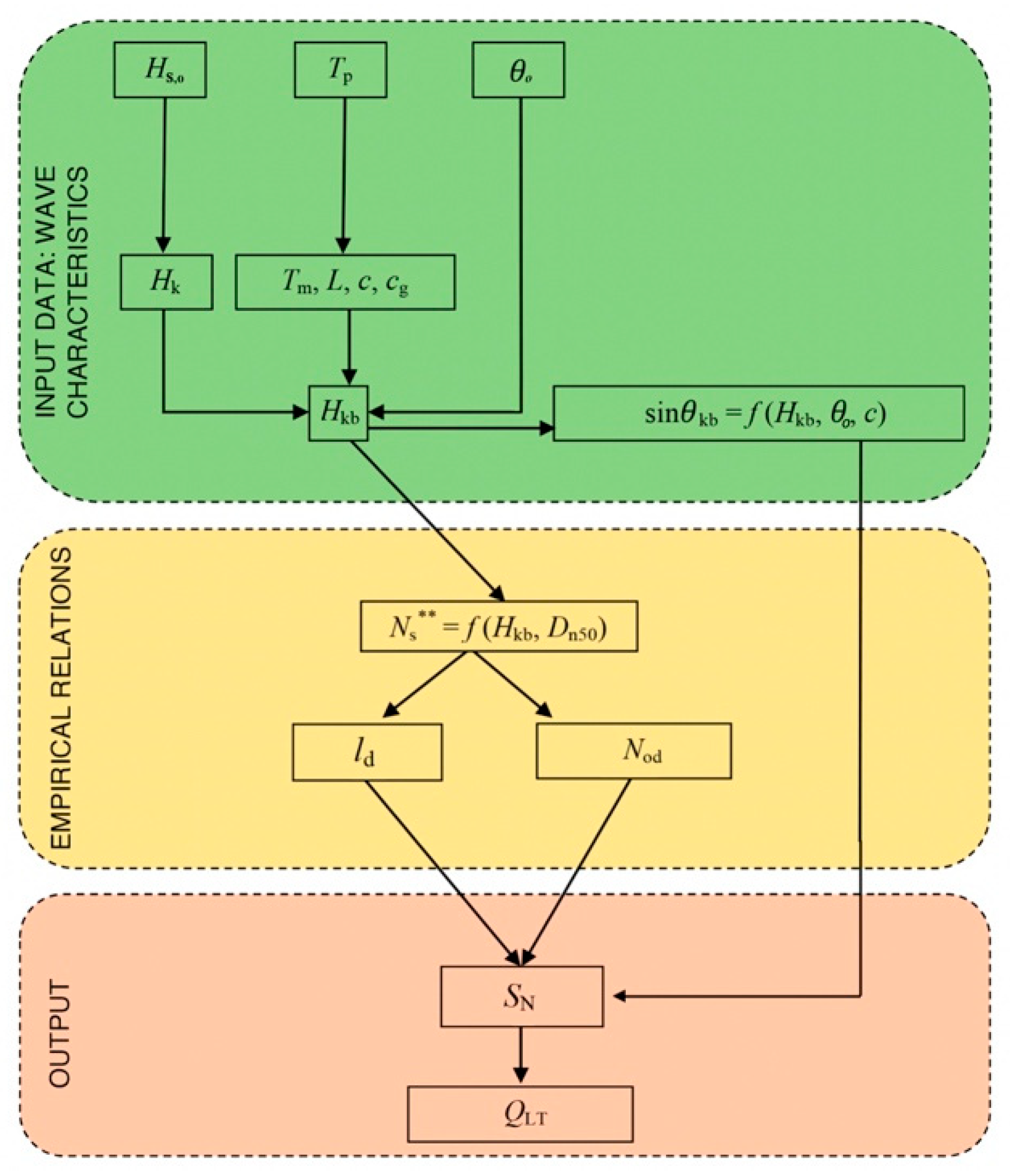
2.1. The General Longshore Transport Model (GLT)
2.2. The General Shoreline Beach Model (GSb)
2.2.1. Theoretical Background
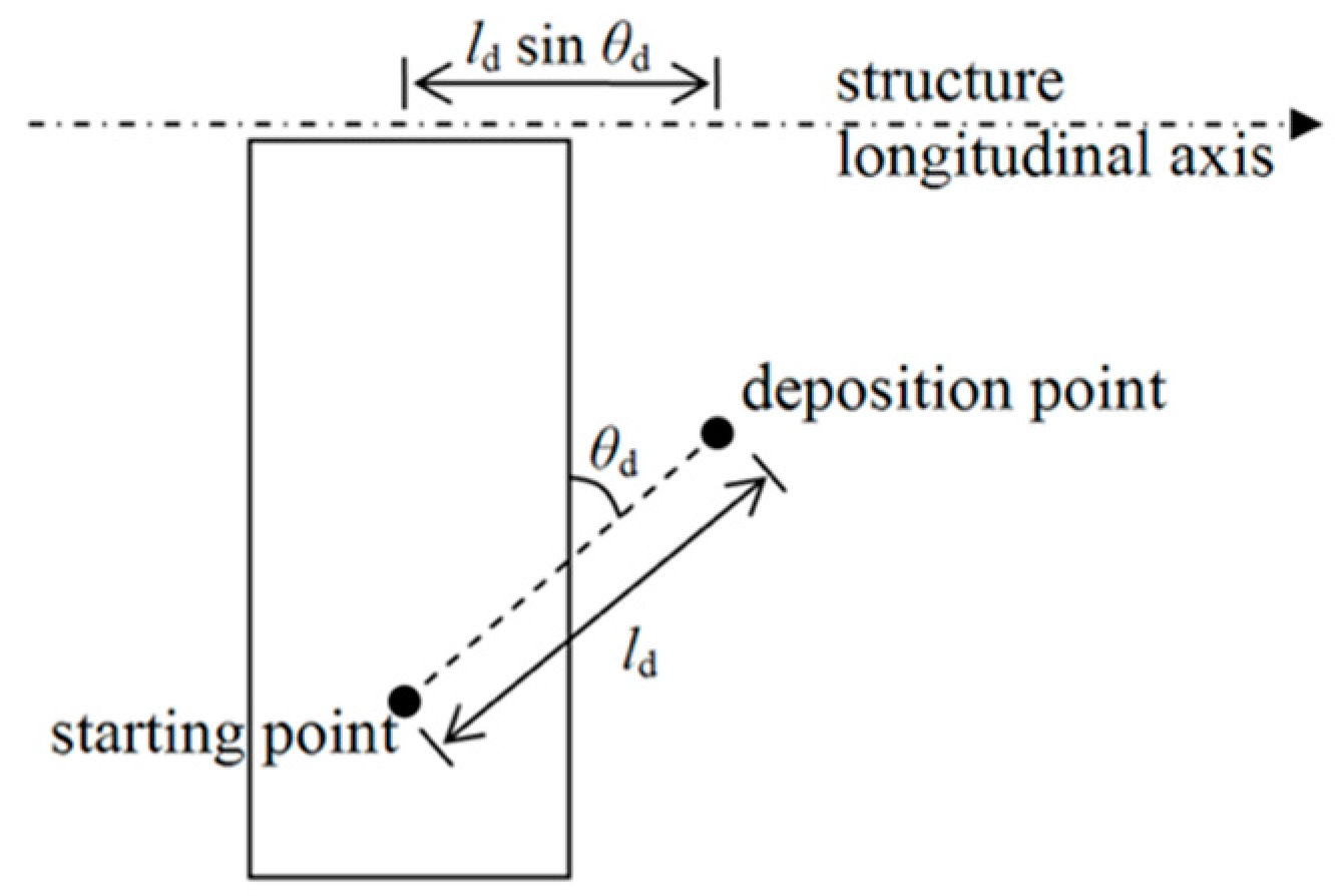
2.2.2. Longshore Sediment Transport Rate
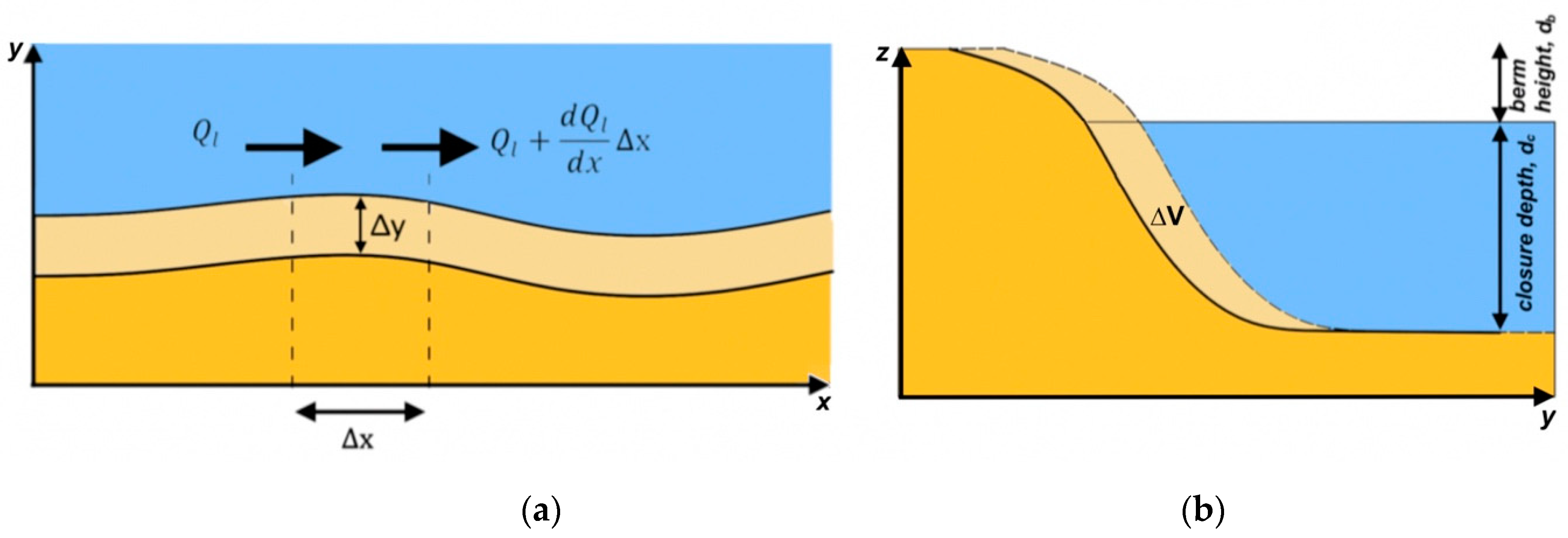
2.2.3. Sediment Continuity Equation
2.3. Influence of Different Inputs
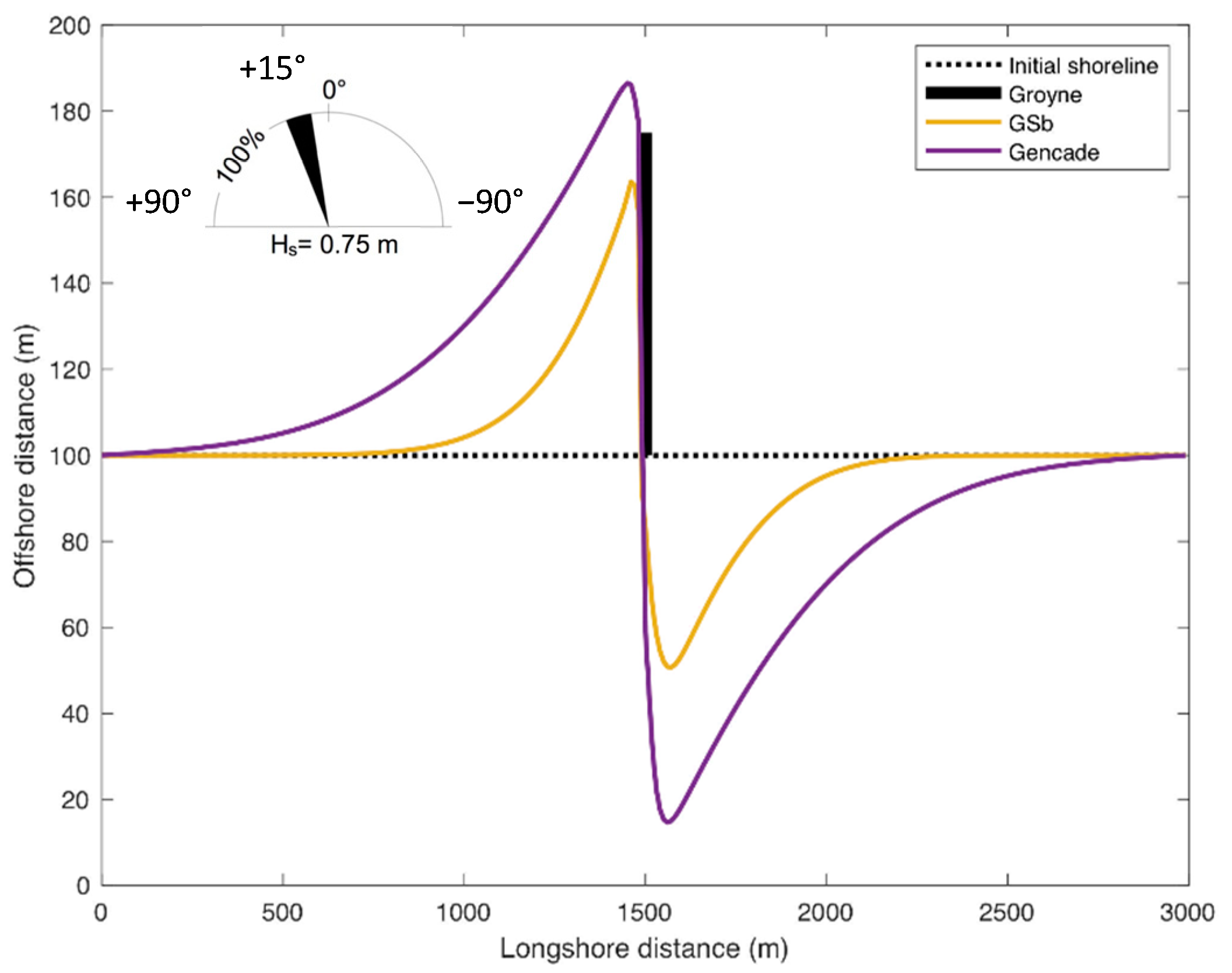
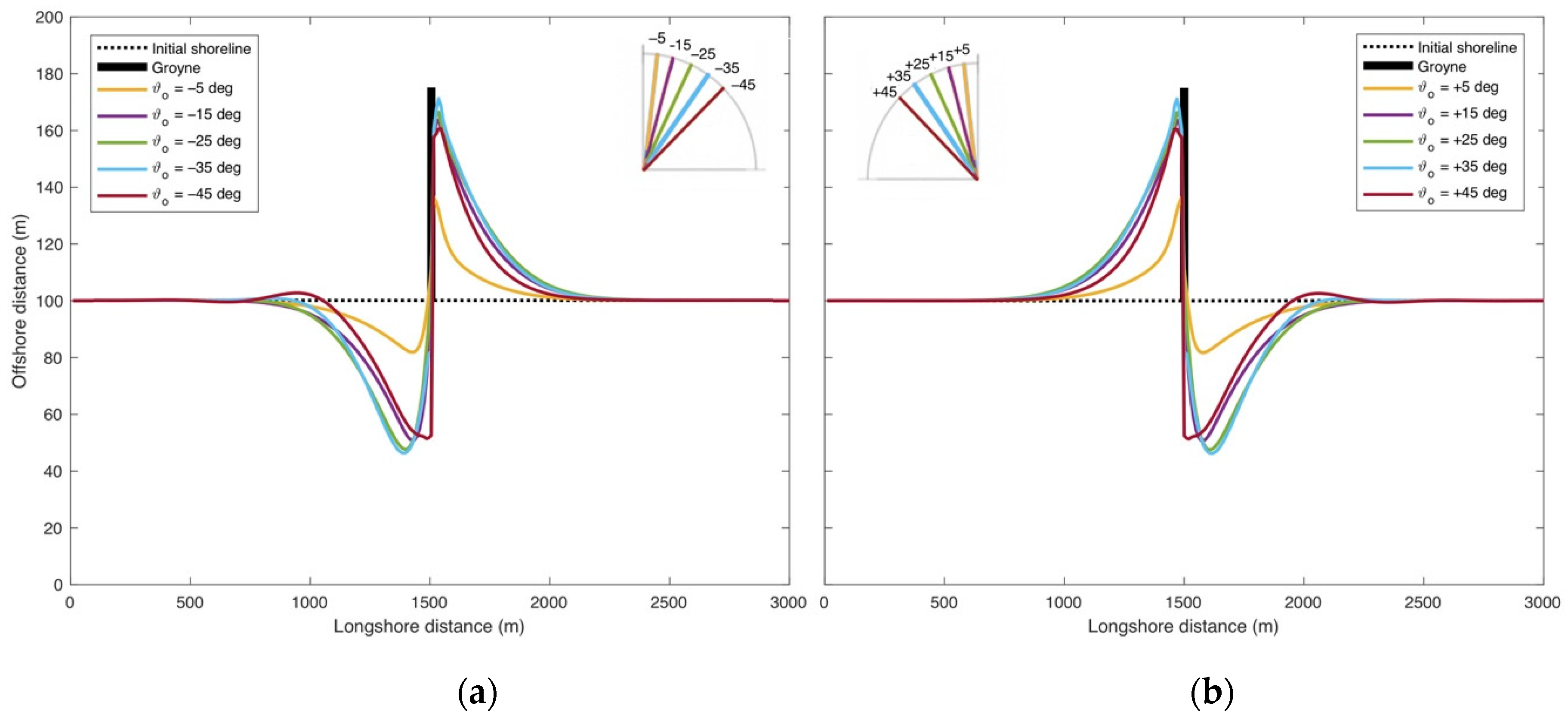
2.3.1. Influence of Offshore Wave Angle
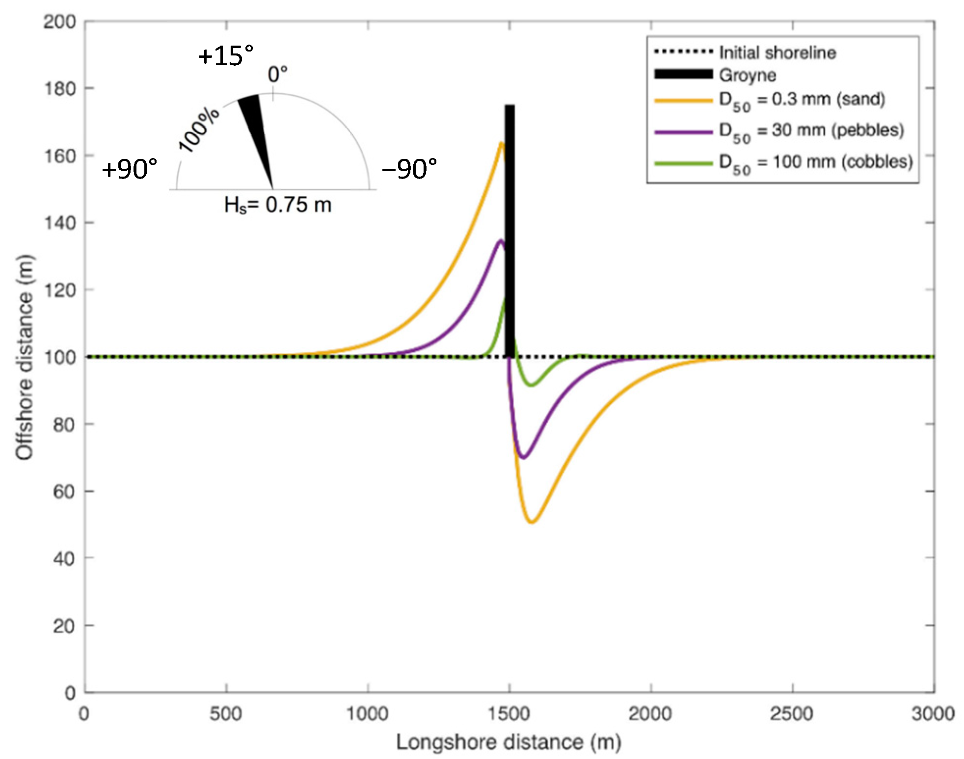
2.3.2. Influence of Nominal Diameter
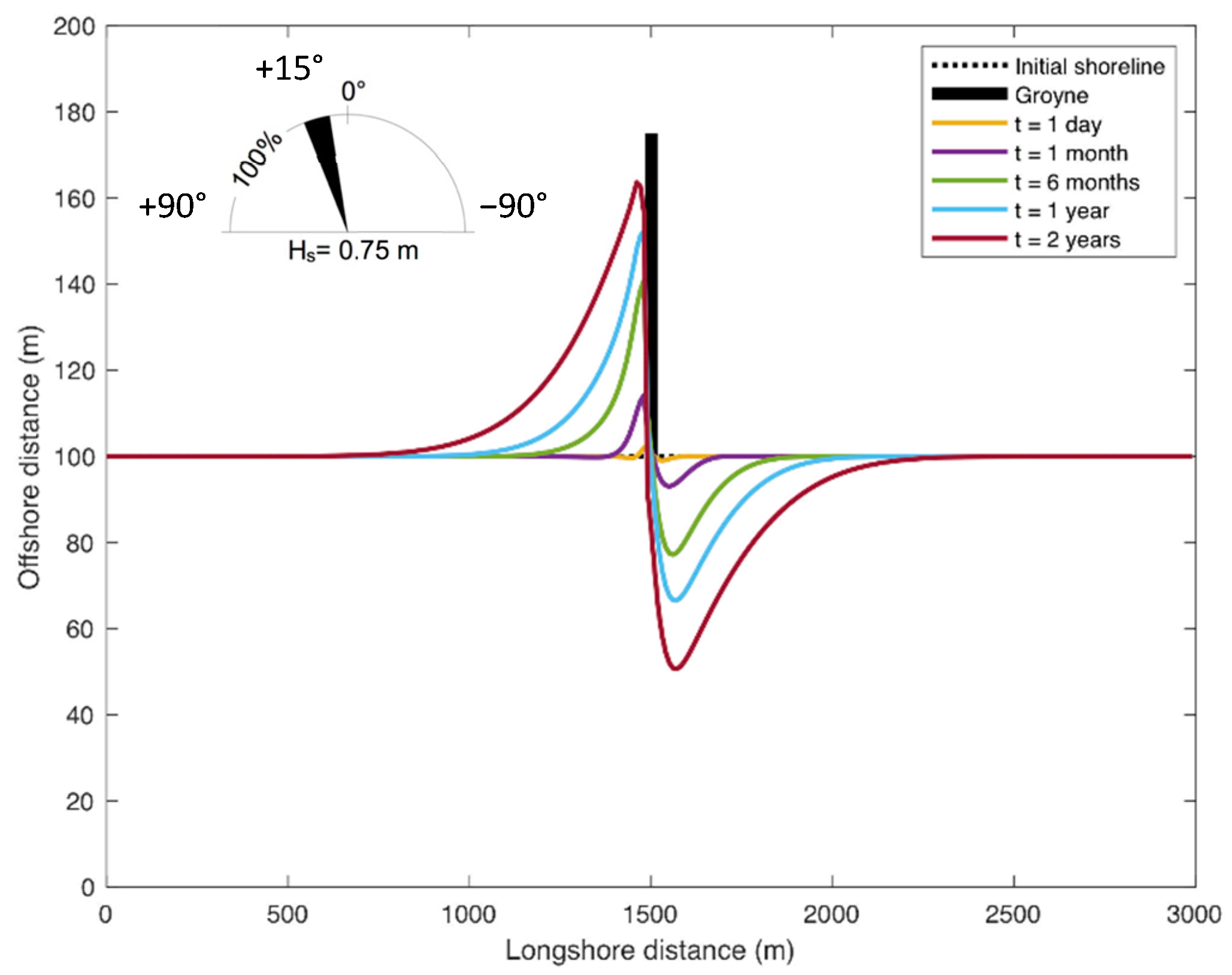
2.3.3. Influence of Duration
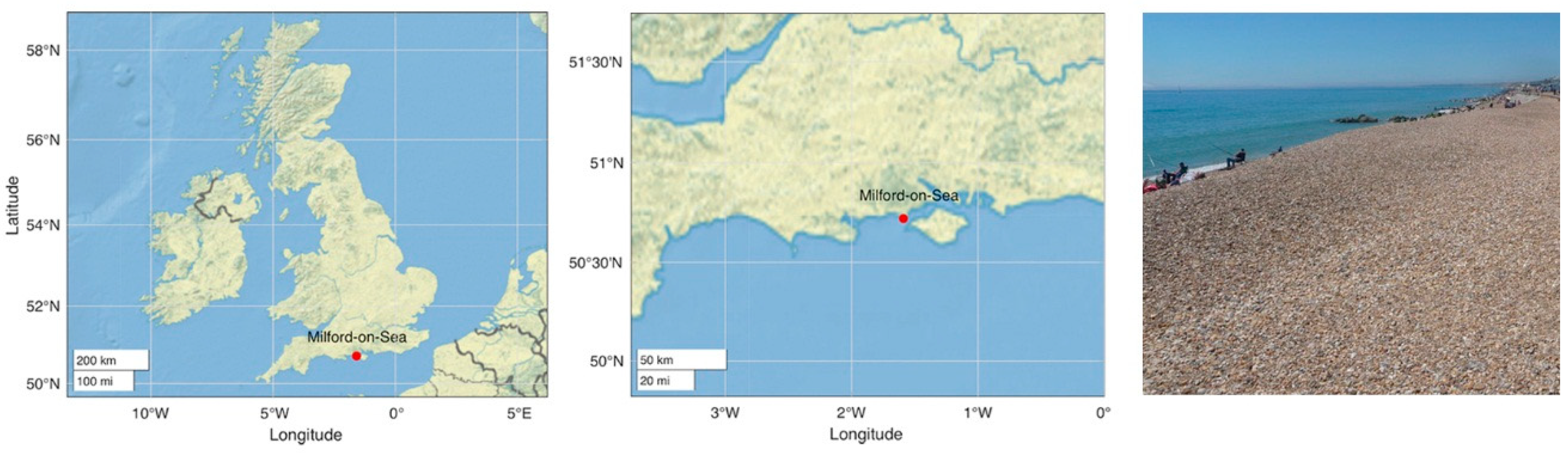
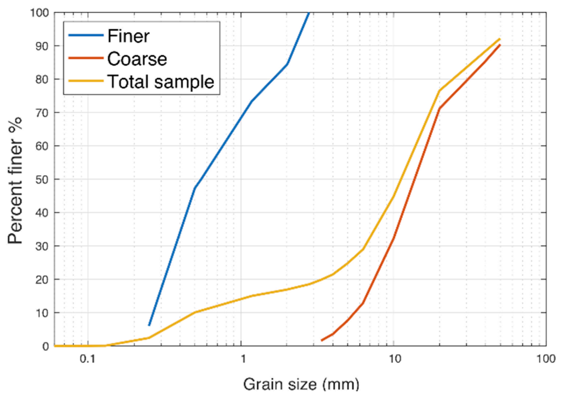
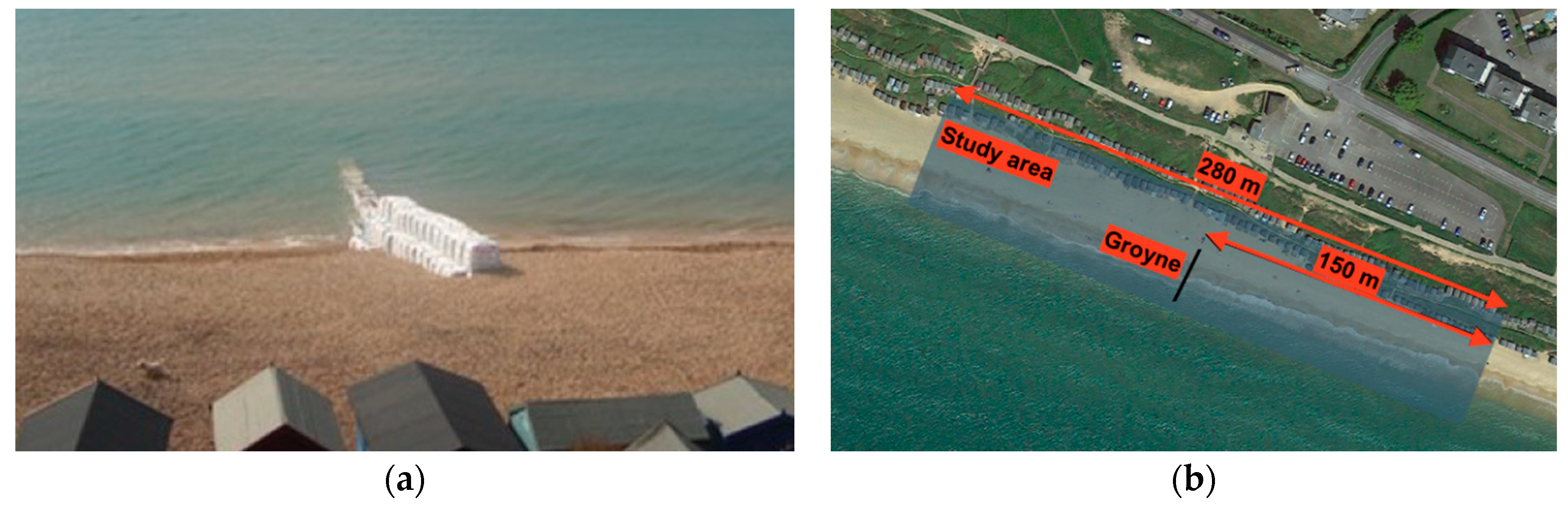
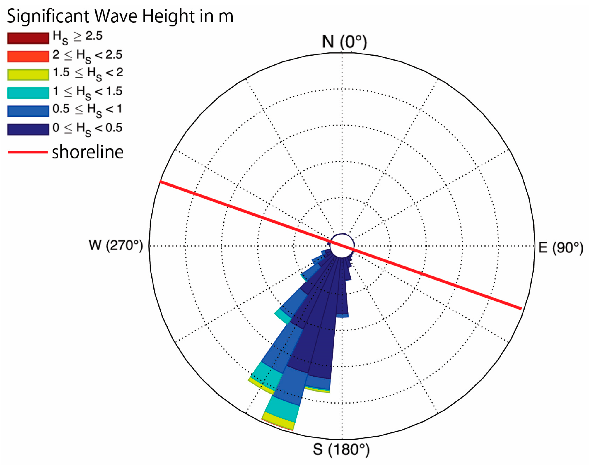
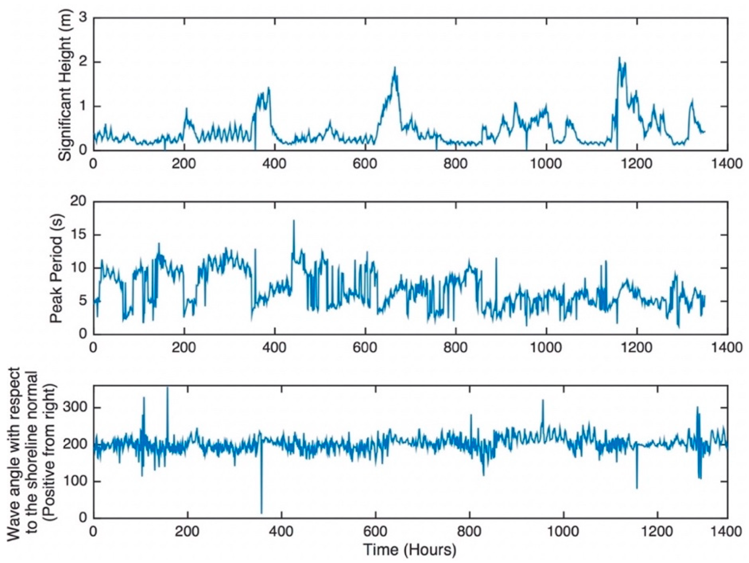
2.4. Field Experiment at a Mixed Beach
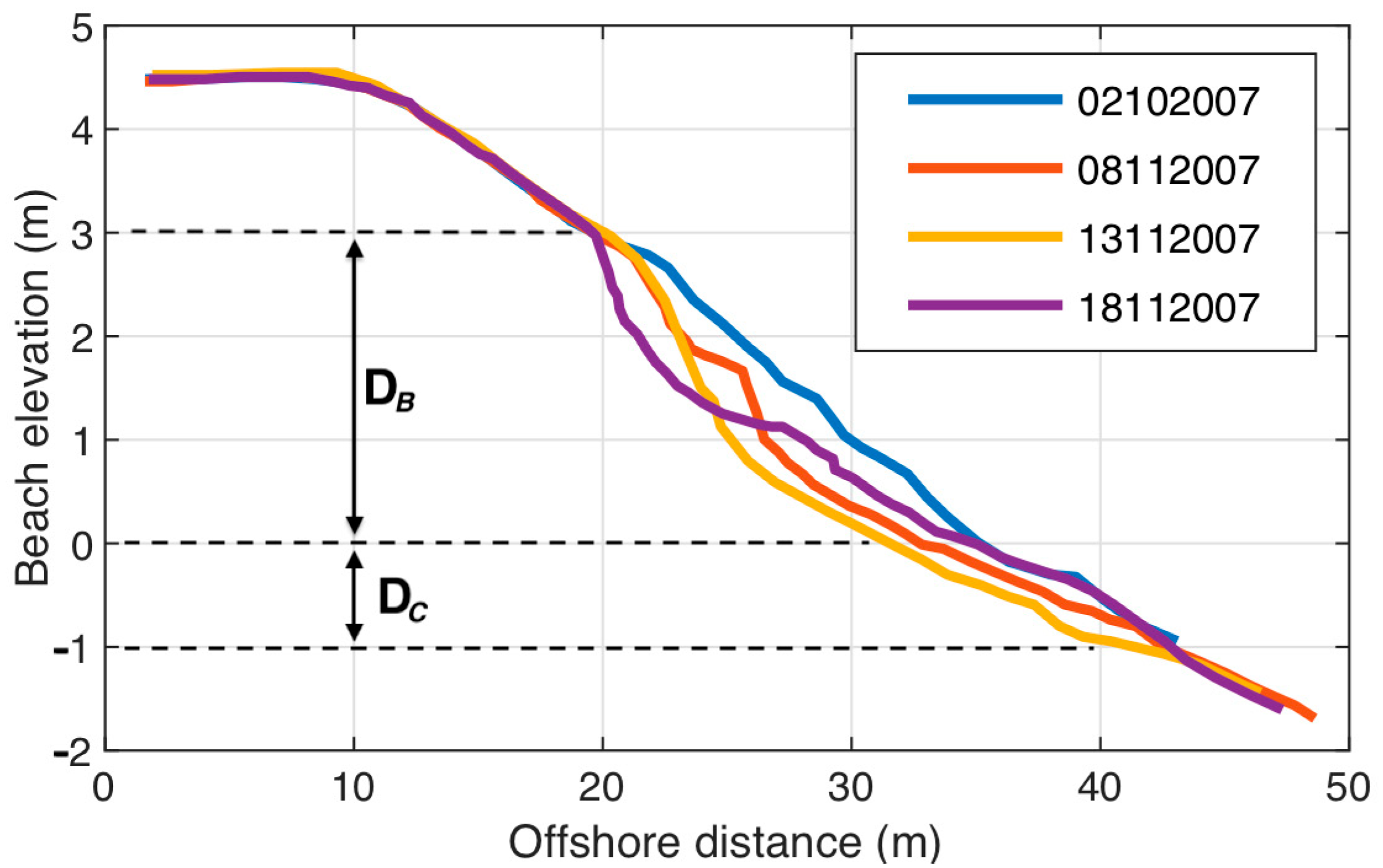
Study Area and Field Observations
3. GSb Calibration and Verification for a Mixed Beach
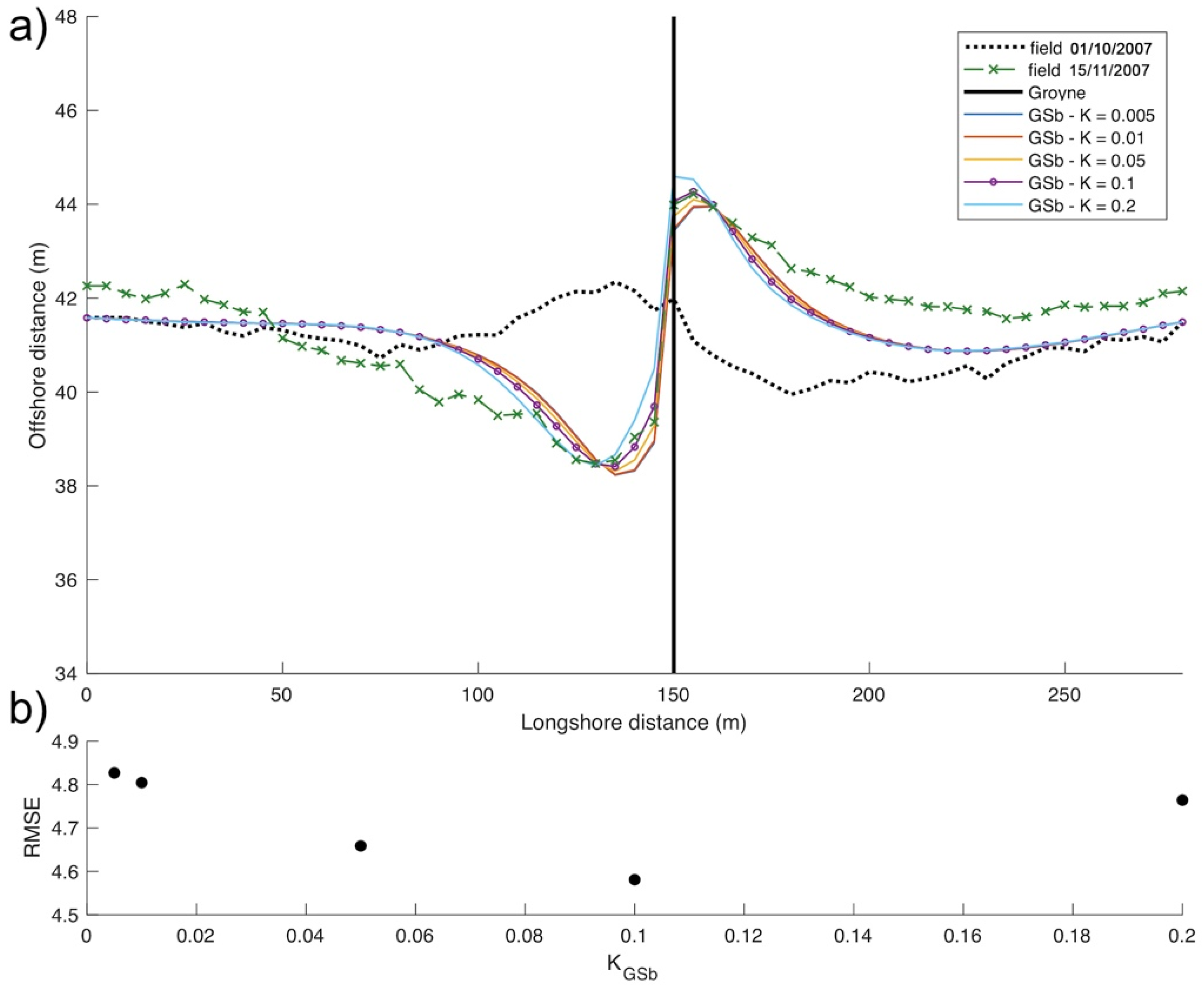
3.1. Calibration
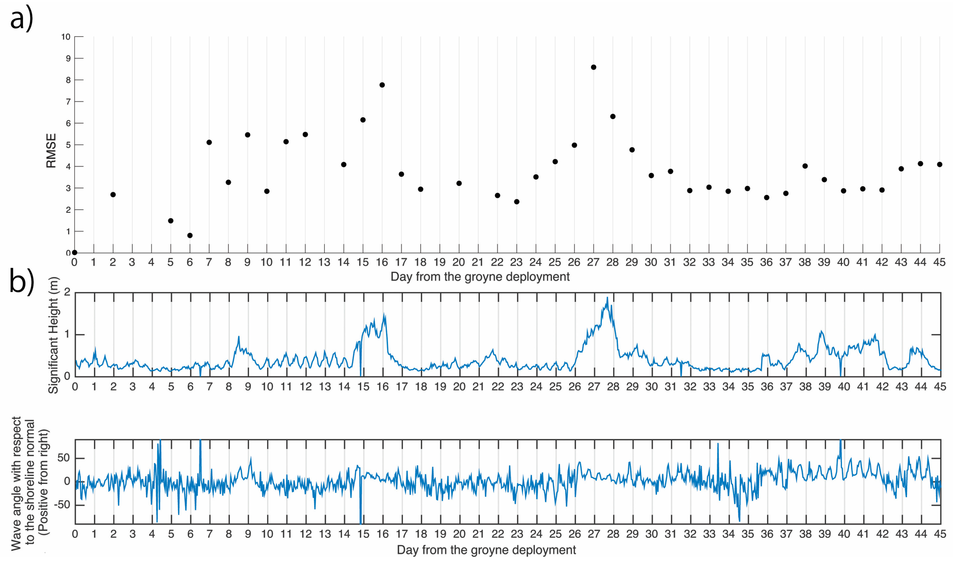
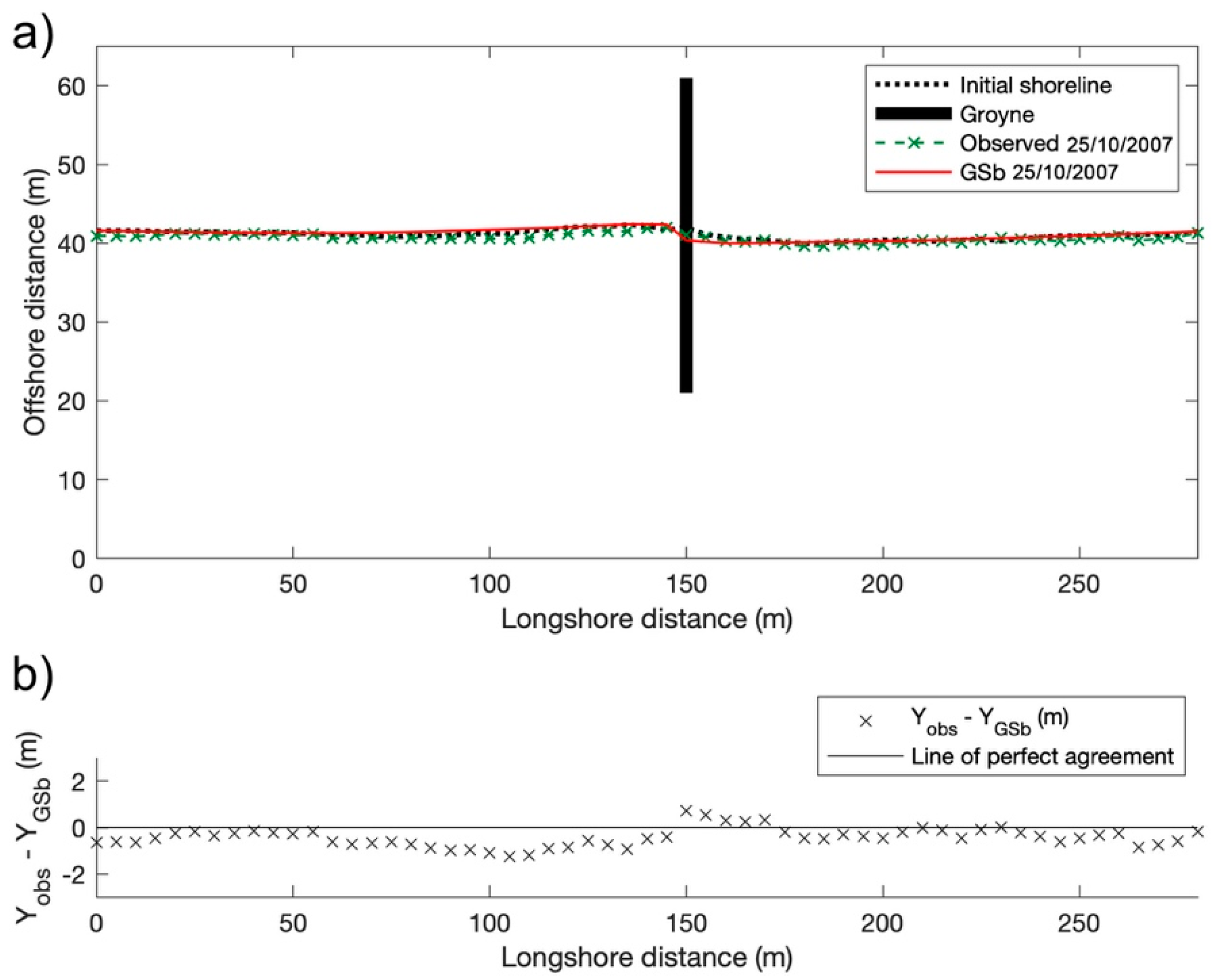
3.2. Verification
4. Conclusions
Supplementary Materials
Author Contributions
Funding
Acknowledgments
Conflicts of Interest
References
- Van Rijn, L.C.; Ribberink, J.S.; Werf, J.V.D.; Walstra, D.J. Coastal sediment dynamics: Recent advances and future research needs. J. Hydraul. Res. 2013, 51, 475–493. [Google Scholar] [CrossRef]
- Güner, H.A.A.; Yüksel, Y.; Çevik, E.Ö. Determination of Longshore Sediment Transport and Modelling of Shoreline Change. Sediment Transp. 2011, 117. [Google Scholar] [CrossRef] [Green Version]
- Hanson, H. GENESIS: A generalized shoreline change numerical model. J. Coast. Res. 1989, 5, 1–27. [Google Scholar]
- Dabees, M.; Kamphuis, J.W. ONELINE, a numerical model for shoreline change. In Proceedings of the 26th Int. Conf. On Coastal Engineering, ASCE, Copenhagen, Denmark, 22–26 June 1998; pp. 2668–2681. [Google Scholar]
- Deltares. UNIBEST-CL+ Manual: Manual for Version 7.1 of the Shoreline Model UNIBEST-CL.; Deltares: Delft, The Netherlands, 2011. [Google Scholar]
- DHI. Litpack: Noncohesive Sediment Transport in Currents and Waves. User Guide; Danish Hydraulic Institute: Hørsholm, Denmark, 2005. [Google Scholar]
- Blanco, B. Beachplan (Version 04.01) Model. Description; HR Wallingford Report; Springer Nature: Berlin/Heidelberg, Germany, 2003. [Google Scholar]
- González, M.; Medina, R.; González-Ondina, J.; Osorio, A.; Méndez, F.; García, E. An integrated coastal modeling system for analyzing beach processes and beach restoration projects, SMC. Comput. Geosci. 2007, 33, 916–931. [Google Scholar] [CrossRef]
- Frey, A.E.; Connell, K.J.; Hanson, H.; Larson, M.; Thomas, R.C.; Munger, S.; Zundel, A. GenCade Version 1 Model. Theory and User’s Guide; Engineer Research And Development Center, Vicksburg Ms Coastal Inlets Research Program: Vicksburg, MS, USA, 2012. [Google Scholar]
- Vionnet, C.; García, M.H.; Latrubesse, E.; Perillo, G. River, Coastal and Estuarine Morphodynamics; RCEM 2009, Two Volume Set; CRC Press: Boca Raton, FL, USA, 2018. [Google Scholar]
- USACE. Shore Protection Manual; Dept. of the Army, Waterways Experiment Station, Corps of Engineers; Coastal Engineering Research Center: Vicksburg, MS, USA, 1984. [Google Scholar]
- Kamphuis, J.W. Alongshore sediment transport rate. J. Waterw. Port Coast. Ocean Eng. 1991, 117, 624–640. [Google Scholar] [CrossRef]
- Bijker, E.W. Longshore transport computations. J. Waterw. Harb. Coast. Eng. Div. 1971, 97, 687–701. [Google Scholar]
- Van Rijn, L.C. Principles of Sediment Transport In Rivers, Estuaries And Coastal Seas; Aqua Publications: Amsterdam, The Netherlands, 1993; Volume 1006. [Google Scholar]
- Bailard, J.A. An energetics total load sediment transport model for a plane sloping beach. J. Geophys. Res. Ocean 1981, 86, 10938–10954. [Google Scholar] [CrossRef]
- DHI. Littoral Processes FM, User Guide; Danish Hydraulic Institute: Hørsholm, Denmark, 2017. [Google Scholar]
- Tomasicchio, G.R.; D‘Alessandro, F.; Musci, F. A multi-layer capping of a coastal area contaminated with materials dangerous to health. Chem. Ecol. 2010, 26, 155–168. [Google Scholar] [CrossRef]
- Bramato, S.; Ortega-Sánchez, M.; Mans, C.; Losada, M.A. Natural Recovery of a Mixed Sand and Gravel Beach after a Sequence of a Short Duration Storm and Moderate Sea States. J. Coast. Res. 2012, 28, 89–101. [Google Scholar] [CrossRef]
- Van Rijn, L.C. A simple general expression for longshore transport of sand, gravel and shingle. Coast. Eng. 2014, 90, 23–39. [Google Scholar] [CrossRef]
- Hanson, H.; Kraus, N.C. Optimization of beach fill transitions. In Proceedings of the Coastal Zone, ASCE, New York, NY, USA, 19–23 July 1993; pp. 103–117. [Google Scholar]
- Van Alphen, J.S.; Hallie, F.P.; Ribberink, J.S.; Roelvink, J.; Louisse, C.J. Offshore sand extraction and nearshore profile nourishment. In Proceedings of the 22nd Coastal Engineering Conference, Delft, The Netherlands, 2–6 July 1991; pp. 1998–2009. [Google Scholar]
- Hamm, L.; Capobianco, M.; Dette, H.; Lechuga, A.; Spanhoff, R.; Stive, M. A summary of European experience with shore nourishment. Coast. Eng. 2002, 47, 237–264. [Google Scholar] [CrossRef]
- Martín-Grandes, I.; Hughes, J.; Simmonds, D.J.; Chadwick, A.J.; Reeve, D.E. Novel methodology for one line model calibration using impoundment on mixed beach. In Proceedings of the Coastal Dynamics 2009: Impacts of Human Activities on Dynamic Coastal Processes, Tokyo, Japan, 7–11 September 2009; World Scientific: Singapore, 2009; pp. 1–10. [Google Scholar]
- Martin-Grandes, I.; Simmonds, D.J.; Karunarathna, H.; Horrillo-Caraballo, J.M.; Reeve, D.E. Assessing the Variability of Longshore Transport Rate Coefficient on a Mixed Beach. In Proceedings of the Coastal Dynamics, Helsingør, Denmark, 12–16 June 2017; pp. 642–653. [Google Scholar]
- Martin-Grandes, I. Understanding Longshore Sediment Transport on a Mixed Beach. Ph.D. Thesis, Plymouth University, Plymouth, UK, 2014. [Google Scholar]
- Lamberti, A.; Tomasicchio, G.R. Stone mobility and longshore transport at reshaping breakwaters. Coast. Eng. 1997, 29, 263–289. [Google Scholar] [CrossRef]
- Tomasicchio, G.R.; D’Alessandro, F.; Frega, F.; Francone, A.; Ligorio, F. Recent improvements for estimation of longshore transport. Ital. J. Eng. Geol. Environ. 2018, 1, 179–187. [Google Scholar]
- Tomasicchio, G.R.; D‘Alessandro, F.; Barbaro, G.; Malara, G. General longshore transport model. Coast. Eng. 2013, 71, 28–36. [Google Scholar] [CrossRef]
- Ahrens, J.P. Characteristics of Reef Breakwaters, (No. CERC-TR-87–17); Coastal Engineering Research Center: Vicksburg, MS, USA, 1987. [Google Scholar]
- Van der Meer, J.W. Rock Slopes and Gravel Beaches under Wave Attack. Ph.D. Thesis, Delft Hydraulics Laboratory, Delft, The Netherlands, 1988. [Google Scholar]
- Klopman, G.; Stive, M. Extreme waves and wave loading in shallow water. In Proceedings of the Wave and Current Kinematics and Loading: E&P Forum Workshop, Paris, France, 25–26 October 1989. [Google Scholar]
- Battjes, J.A.; Groenendijk, H.W. Wave height distributions on shallow foreshores. Coast. Eng. 2000, 40, 161–182. [Google Scholar] [CrossRef]
- Komar, P.D.; Gaughan, M.K. Airy wave theory and breaker height prediction. In Proceedings of the 13th Conf. on Coastal Engineering, Vancouver, Canada, 29 January 1972; pp. 405–418. [Google Scholar]
- Tomasicchio, G.; Lamberti, A.; Guiducci, F. Stone movement on a reshaped profile. In Proceedings of the 24th International Conf. on Coastal Engineering, ASCE, Kobe, Japan, 23–28 October 1994; pp. 1625–1640. [Google Scholar]
- Tørum, A.; Sigurdarson, S. PIANC Working Group No. 40: Guidelines for the Design and Construction of Berm Breakwaters. In Proceedings of the Breakwaters, Coastal Structures and Coastlines, London, UK, 26–28 September 2001; pp. 373–384. [Google Scholar]
- Pelnard-Considere, R. Essai de theorie de l’evolution des formes de rivage en plages de sable et de galets. In Proceedings of the Les Energies de la Mer: Compte Rendu Des. Quatriemes Journees de L’hydraulique, Paris, France, 13–15 June 1956. rapport 1, 74-1-10. [Google Scholar]
- Bruun, P. Coast. Erosion and the Development of Beach Profiles; US Beach Erosion Board: Washington, DC, USA, 1954; Volume 44. [Google Scholar]
- Dean, R.G. Equilibrium Beach Profiles: US Atlantic and Gulf Coasts; Department of Civil Engineering and College of Marine Studies, Newark, University of Delaware: Newark, DE, USA, 1977. [Google Scholar]
- Hanson, H.; Kraus, N.C. GENESIS: Generalized Model. for Simulating Shoreline Change. Report 1. Technical Reference; Coastal Engineering Research Center: Vicksburg, MS, USA, 1989. [Google Scholar]
- Tomasicchio, G.R.; D’Alessandro, F.; Barbaro, G.; Musci, E.; De Giosa, T.M. Longshore transport at shingle beaches: An independent verification of the general model. Coast. Eng. 2015, 104, 69–75. [Google Scholar] [CrossRef]
- Hanson, H. GENESIS: A Generalized Shoreline Change Numerical Model for Engineering Use; Department of Water Resources Engineering, Lund University: Lund, Sweden, 1987. [Google Scholar]
- Ozasa, H.; Brampton, A. Mathematical modelling of beaches backed by seawalls. Coast. Eng. 1980, 4, 47–63. [Google Scholar] [CrossRef]
- Medellín, G.; Torres-Freyermuth, A.; Tomasicchio, G.R.; Francone, A.; Tereszkiewicz, P.A.; Lusito, L.; Palemón-Arcos, L.; López, J. Field and numerical study of resistance and resilience on a sea breeze dominated beach in Yucatan (Mexico). Water 2018, 10, 1806. [Google Scholar] [CrossRef] [Green Version]
- Hamza, W.; Tomasicchio, G.R.; Ligorio, F.; Lusito, L.; Francone, A. A Nourishment Performance Index for Beach Erosion/Accretion at Saadiyat Island in Abu Dhabi. J. Mar. Sci. Eng. 2019, 7, 173. [Google Scholar] [CrossRef] [Green Version]
- Hallermeier, R.J. Sand transport limits in coastal structure designs. In Proceedings of the Coastal Structures’ 83, Washington, DC, USA, 9–11 March 1983; pp. 703–716. [Google Scholar]
- Goda, Y.; Takayama, T.; Suzuki, Y. Diffraction Diagrams for Directional Random Waves. In Proceedings of the 16th International Conference on Coastal Engineering, Hamburg, Germany, 27 August–3 September 1978; Volume 1. [Google Scholar]
- Larson, M. Numerical modeling. In Encyclopedia of Coastal Science; Schwartz, M., Ed.; Springer: Dordrecht, The Netherlands, 2005; pp. 730–733. [Google Scholar]
- Bodge, K.R.; Dean, R.G. Short-term impoundment of longshore transport. In Proceedings of the Coastal Sediments, New Orleans, Louisiana, 12–14 May 1987; pp. 468–483. [Google Scholar]
- Wang, P.; Kraus, N.C. Longshore sediment transport rate measured by short-term impoundment. J. Waterw. Port Coast. Ocean Eng. 1999, 125, 118–126. [Google Scholar] [CrossRef] [Green Version]
- Van Wellen, E.; Chadwick, A.; Mason, T. A review and assessment of longshore sediment transport equations for coarse-grained beaches. Coast. Eng. 2000, 40, 243–275. [Google Scholar] [CrossRef]


| Model | Variability of Seabed Proprieties | Diffraction Around the Structures | Longshore Current | Longshore Sediment Transport | Groynes | Detached Breakwaters |
|---|---|---|---|---|---|---|
| GENESIS | No | Yes | No | CERC [11] | Yes | Yes |
| ONELINE | No | Yes | No | Kamphuis [12] | Yes | Yes |
| UNIBEST | No | No | Yes | Bijker [13] Van Rijn [14] Bailard [15] CERC [11] | Yes | No |
| LITPACK | Yes | Yes | Yes | STPQ3D [16] | Yes | Yes |
| BEACHPLAN | Yes | Yes | Yes | CERC [11] | Yes | Yes |
| SMC | No | Yes | No | CERC [11] | No | No |
| GENCADE | No | Yes | No | CERC [11] | Yes | Yes |
| Dn50 (mm) | 0.3 |
| DB (m) | 1 |
| DC (m) | 8 |
| Hs,o (m) | 0.75 |
| Tp (s) | 8 |
| (deg) | 15 |
| DX (m) | 10 |
| NX (-) | 300 |
| DT (h) | 0.5 |
| t (years) | 2 |
| KGSb (-) | 0.25 |
© 2020 by the authors. Licensee MDPI, Basel, Switzerland. This article is an open access article distributed under the terms and conditions of the Creative Commons Attribution (CC BY) license (http://creativecommons.org/licenses/by/4.0/).
Share and Cite
Tomasicchio, G.R.; Francone, A.; Simmonds, D.J.; D’Alessandro, F.; Frega, F. Prediction of Shoreline Evolution. Reliability of a General Model for the Mixed Beach Case. J. Mar. Sci. Eng. 2020, 8, 361. https://doi.org/10.3390/jmse8050361
Tomasicchio GR, Francone A, Simmonds DJ, D’Alessandro F, Frega F. Prediction of Shoreline Evolution. Reliability of a General Model for the Mixed Beach Case. Journal of Marine Science and Engineering. 2020; 8(5):361. https://doi.org/10.3390/jmse8050361
Chicago/Turabian StyleTomasicchio, Giuseppe R., Antonio Francone, David J. Simmonds, Felice D’Alessandro, and Ferdinando Frega. 2020. "Prediction of Shoreline Evolution. Reliability of a General Model for the Mixed Beach Case" Journal of Marine Science and Engineering 8, no. 5: 361. https://doi.org/10.3390/jmse8050361