
Abstract
HEPfit is a flexible open-source tool which, given the Standard Model or any of its extensions, allows to (i) fit the model parameters to a given set of experimental observables; (ii) obtain predictions for observables. HEPfit can be used either in Monte Carlo mode, to perform a Bayesian Markov Chain Monte Carlo analysis of a given model, or as a library, to obtain predictions of observables for a given point in the parameter space of the model, allowing HEPfit to be used in any statistical framework. In the present version, around a thousand observables have been implemented in the Standard Model and in several new physics scenarios. In this paper, we describe the general structure of the code as well as models and observables implemented in the current release.
1 Introduction
Searching for New Physics (NP) beyond the Standard Model (SM) in the era of the Large Hadron Collider (LHC) requires combining experimental and theoretical information from many sources to optimize the NP sensitivity. NP searches, even in the absence of a positive signal, provide useful information which puts constraints on the viable parameter space of any NP model. Should a NP signal emerge at future LHC runs or elsewhere, the combination of all available information remains a crucial step to pin down the actual NP model. NP searches at the LHC require extensive detector simulations and are usually restricted to a subset of simplified NP models. Given the high computational demand of direct searches, it is crucial to explore only regions of the parameter space compatible with other constraints. In this respect, indirect searches can be helpful and make the study of more general models viable.
HEPfit aims at providing a tool which allows to combine all available information to select allowed regions in the parameter space of any NP model. To this end, it can compute many observables with state-of-the-art theoretical expressions in a set of models which can be extended by the user. It also offers the possibility of sampling the parameter space using a Markov Chain Monte Carlo (MCMC) implemented using the BAT library [1,2,3]. Alternatively, HEPfit can be used as a library to obtain predictions of the observables in any implemented model. This allows to use HEPfit in any statistical framework.
HEPfit is written in C++ and parallelized with MPI. This is the first public release with a limited set of observables and models, which we plan to enlarge. The code is released under the GNU General Public License, so that contributions from users are possible and welcome. In particular, the present version provides Electroweak Precision Observables (EWPO), Higgs signal strengths, and several flavour observables in the SM, in Two-Higgs-Doublet Models (THDM), and in several parameterizations of NP contributions. Furthermore, it also calculates various Lepton Flavour Violating (LFV) observables in the Minimal Supersymmetric Standard Model (MSSM). In the near future, we plan to add many more observables and to enlarge the spectrum of NP models.
The paper is organized as follows. In Sect. 2 we give a brief description of HEPfit including the statistical framework used, the MPI parallelization and some other details. In Sect. 3 we discuss the models implemented in HEPfit. In Sect. 4 we go on discussing some of the observables implemented in HEPfit. In Sect. 5 we present some physics results obtained using HEPfit in previous publications. Indeed several physics analyses [4,5,6,7,8,9,10,11,12,13,14,15,16,17,18,19,20,21,22,23,24,25,26,27,28,29,30] have been completed using HEPfit and serve as a validation of the code and of its use as an open-source computational framework. A detailed description of the installation procedure can be found in Sect. 6 followed by examples of how to use HEPfit in Sect. 7. Updated information and detailed online documentation can be found on the HEPfit website [31].
2 The HEPfit code
HEPfit is a computational tool for the combination of indirect and direct constraints on High Energy Physics models. The code is built in a modular structure so that one can pick and choose which observables to use and what model to analyze. It also provides an interface that can be used to build customized models along with customized observables. This flexible framework allows defining a model of choice and observables that depend on the parameters of this model, thus opening up the possibility of using HEPfit to perform phenomenological analyses in such a model.
The tool comes with a built-in statistical framework based on a Bayesian MCMC analysis. However, any statistical framework can be used along with this tool since a library is made available. HEPfit also allows for the incorporation of parametric and experimental correlations and can read likelihood distributions directly from ROOT histograms. This removes the necessity for setting experimental constraints through parameterized distributions which might require making approximations.
Since the statistical core of HEPfit is based on a MCMC, speed of computation is of utmost importance. HEPfit is already massively parallelized to run over large number of CPUs using OpenMPI and scales well to hundreds of processing units. The framework further brings forth the flexibility of defining a model of choice and observables that depend on the parameters of this model, thus opening up the possibility of performing various analyses using HEPfit.
The package comes with several examples of how HEPfit can be used and detailed documentation of the code and the physics can be found online on the HEPfit website. Throughout its development, emphasis has been placed on speed and streamlining error handling. HEPfit has been tested through several analyses on various hardware architecture and displays reliable scaling to large systems.
2.1 Statistical framework
HEPfit can be used both as a library to compute the values of chosen observables and also as a MCMC based Bayesian analysis framework. While the former approach allows for choosing the statistical framework one wants to use, the latter uses a robust Bayesian MCMC framework implemented in the public code BAT [1,2,3]. In this section we give a brief overview of the Bayesian statistical framework implemented in HEPfit using BAT.
2.1.1 Bayesian framework
Once the model parameters, \(\vec {{\mathbf {x}}}\), and the data, D, are defined one can define the posterior distribution according to Bayes theorem as:
where \(P_0(\vec {{\mathbf {x}}})\) is the prior distribution of the parameters which represents the prior knowledge of the parameters which can come from experiments or theory computations or can be uninformative. The denominator is called the normalization or the evidence, the computation of which can allow for model comparison through the Bayes factor. The likelihood is denoted as \(P(D|\vec {{\mathbf {x}}})\). Once the (unnormalized) posterior distributionFootnote 1 is mapped out using sampling methods (in our case a MCMC routine), one can obtain the marginalized posterior distributions of the individual parameters from which the credibility regions can be computed. The 1D marginalized distribution is given by
where all the variables but the one for which the marginalized posterior distribution is being computed are integrated over, and similarly for marginalized 2D distributions.
2.1.2 Markov chain Monte Carlo
In general, the posterior distribution specified in Eq. (2.1) cannot be computed easily, especially when there is a proliferation of model parameters. Using a naive Monte Carlo sampling algorithm can lead to unacceptable execution times because of the inherent inefficiency in sampling the parameter space. However, MCMC procedures overcome this hurdle and make the application of Bayes theorem quite tractable.
The implementation of MCMC in BAT uses a Metropolis-Hastings algorithm to sample the parameter space from the posterior. The steps of a Metropolis-Hastings algorithm for sampling from a (unnormalized) probability density \(f(\vec {{\mathbf {x}}})\) are as follows:
- 1.
Start at a random point in the parameter space \(\vec {{\mathbf {x}}}\).
- 2.
Generate a proposal point \(\vec {{\mathbf {y}}}\) according to a symmetric probability distribution \(g(\vec {{\mathbf {x}}},\vec {{\mathbf {y}}})\).
- 3.
Compare the value of the function f at proposal point \(\vec {{\mathbf {y}}}\) with the value at the current point \(\vec {{\mathbf {x}}}\). The proposal point is accepted if:
\(f(\vec {{\mathbf {y}}}) \ge f(\vec {{\mathbf {x}}})\),
otherwise, generate a random number r from a uniform distribution in the range [0, 1] and accept the proposal if \(f(\vec {{\mathbf {y}}})/f(\vec {{\mathbf {x}}}) > r\).
If neither conditions are satisfied the proposal is rejected.
- 4.
Continue from step 1.
In our case, the function \(f(\vec {{\mathbf {y}}})\) is the unnormalized posterior, namely the numerator of Eq. (2.1).
The MCMC implementation consists of two parts. The first part is called the pre-run or the burn-in phase where the chains start from arbitrary random points in the parameter space and reach a stationary state after a certain number of iterations, through the tuning of the proposal function. The stationary state is reached once the targeted efficiency of the proposal and R-values close to one are obtained. The R-value for a parameter is essentially the distance of its mean values in the various chains in units of the standard deviation of the parameter in each chain [32, 33]. Samples of the parameter space are not collected during the pre-run. Once the pre-run is over, the samples of the parameter space are collected in the main run to get the marginalized distributions of all the parameters and the corresponding posterior distributions of the observables and of any other derived quantity that may have been defined. The details of the implementation of the MCMC framework can be found in Refs. [1,2,3].
In our work we have not faced any limitations to the number of parameters that can be used and the number of observables that can be used in the fit. However, one has to take note of the following regarding the time taken for the fits:
The convergence of the Markov chains is slower for larger number of parameters and when the parameters are correlated explicitly or as a consequence of the data used as observables for both factorized and non-factorized priors. To reduce the time of the fit it is best to reduce the number of parameters to the minimum necessary.
For larger number of parameters (> 30) it is advised to compare fits using both the factorized and non-factorized priors for optimal performance (see Sect. 7 for details).
There is no limitation to the number of observables that can be defined. However, if the observables are computationally expensive, they will slow the fits accordingly.
The largest fits that we have performed with HEPfit contained more than 90 free parameters and more than 200 observables. Other fits have been done with several hundred observables but smaller number of parameters. We have not seen any limitation from these other than the time consumed to do the fits, which are at most a few days as shown in Table 1.
2.1.3 Integration of BAT with HEPfit
The MCMC framework implemented in BAT is integrated in HEPfit using the library that is provided by BAT on compilation. The MonteCarloEngine class in HEPfit inherits from the BCModel class in BAT and overloads the LogLikelihood function. This method generates the numerical likelihood for one point in the parameter space with the values of the observables computed by HEPfit and the experimental and theoretical constraints provided to HEPfit. The parameters and their distributions are passed by HEPfit to BAT through the MonteCarloEngine class. HEPfit takes care of correlated parameter priors by rotating them to the eigenvector basis in order to increase the efficiency of sampling.
The output of a run, as detailed in Sect. 7.1, is produced by both BAT and HEPfit. All 1D and 2D marginalized distributions and posterior distributions are produced using the BCH1D and the BCH2D classes of BAT and stored in a ROOT file. One can choose to store the chains in the ROOT file as well using HEPfit. While this is useful for post-processing, since it makes the full sample available point by point, it entails a dramatic increase in size of the output ROOT file.
It should be noted that BAT is necessary only when running in the MCMC mode. If one chooses to run HEPfit as an event generator or to only compute values of observables for custom statistical analyses, the interface with BAT is not used at all.
2.2 Parallelization with MPI
One of the most important advantages of HEPfit over several other similar publicly available codes is that it is completely parallelized using OpenMPI, allowing it to be run on both single CPUs with multiple cores and on several nodes on large clusters. The MCMC algorithm is very apt for this kind of parallelization since an integer number of chains can be run on each core. Ideally allocating one core per chain minimizes the run time.
The official version of BAT is parallelized using OpenMP. However, OpenMP relies on shared memory and cannot be distributed over several nodes in a cluster. To overcome this limitation we used OpenMPI to parallelize both BAT and HEPfit. The parallelization is at the level of the computation of likelihood and observables. This means that the MCMC at both the pre-run and main run stages can take advantage of this parallelization. Once the likelihood computation (which requires the computation of the observables) is done, the flow is returned to the master, which performs the generation of the next set of proposal points. The computation of efficiencies and convergence, as well as the optimization of the proposal function, are currently not distributed since they require full information on the chain states. This is the only bottleneck in the parallelization, since the time the master takes to process these steps might be comparable to the time required to compute all the observables by each chain, if the number of chains is very large. However, this begins to be a matter of concern only when the number of chains is in the range of several hundreds, a situation that a normal user is unlikely to encounter.
To demonstrate the advantages that one can get from the parallelization built into HEPfit and to give an estimate of the scaling of the run-times with the number of cores, we give some examples of analyses that can be done both on personal computers and on large clusters in Table 1. These should not be taken as benchmarks since we do not go into the details of the hardware, compiler optimization, etc. Rather, these should be taken as an indication of how MPI parallelization greatly enhances the performance of the HEPfit code.
2.3 Custom models and observables
Another unique feature that HEPfit offers is the possibility of creating custom models and custom observables. All the features of HEPfit are made available along with all the observables and parameters predefined in HEPfit. An example of such a use of HEPfit can be found in Ref. [23]. Detailed instructions for implementation are given in Sect. 7.4.
The user can define a custom model using a template provided with the package, by adding a set of parameters to any model defined in HEPfit. Generally, in addition to defining the new parameters, the user should also specify model-specific additional contributions to any observables predefined in HEPfit that he wants to use. Furthermore, new observables can be defined in terms of these new parameters.
New observables can also be defined in the context of the predefined HEPfit models. In this case, the user just needs to specify the observable in terms of the model parameters, without the need to create a custom model. The parameters already used in HEPfit can also be accessed. For example, one does not need to redefine the Cabibbo–Kobayashi–Maskawa (CKM) mixing matrix, \(V_{\mathrm {CKM}}\), if one needs to use it in the computation of a custom observable. One can simply call the SM object available to all observables and then use the implementation of \(V_{\mathrm {CKM}}\) already provided either in terms of the Wolfenstein parameters or in terms of the elements of the matrix. It should be noted that one does not need to define a custom model to define custom observables. A custom model should be defined only if the user requires parameters not already present in HEPfit. More details can be found in Sect. 7.4.
3 Models defined in HEPfit
The basic building blocks of HEPfit are the classes Model and Observable. Actual models extend the base class Model sequentially (e.g. QCD \(\leftarrow \) StandardModel \(\leftarrow \) THDM \(\leftarrow \) ...). Inheritance allows a given model to use all the methods of the parent ones and to redefine those which have to include additional contributions specific to the extended model. For example, the method computing the strong coupling constant (\(\alpha _s\)) includes strong corrections in QCD, adds electromagnetic corrections in StandardModel, and any additional contributions in classes extending the StandardModel. Models contain model parameters (both fundamental model parameters and auxiliary ones) and model flags which control specific options.
An instance of the Observable class contains the experimental information relative to a given physical observable as well as an instance of the class ThObservable, responsible for the computation of that observable in the given model. This is the class where both the experimental or theoretical constraints and the theory computation in the model are accessible, allowing for the likelihood calculation. We now briefly review the models implemented in the current release of HEPfit.
3.1 The Standard Model
In HEPfit, the minimal model to be defined in order to compute any observable is the StandardModel, which for convenience extends a class QCD, which in turn, extends the abstract class Model.
The model implemented in the QCD class defines the following model parameters: the value of \(\alpha _s(M)\) at a provided scale M, the \(\overline{\mathrm {MS}}\) quark masses \({{\bar{m}}}_q\) (except for the top quark mass where for convenience the pole mass is taken as input parameter and then converted to \(\overline{\mathrm {MS}}\)). With this information, the class initializes instances of the \(\texttt {Particle}\) class for each quark. In addition, objects of type \(\texttt {Meson}\), containing information on masses, lifetimes, decay constants and other hadronic parameters (these are taken as model parameters although in principle they are derived quantities), are instantiated for several mesons. Furthermore, bag parameters for meson mixings and decays are instantiated. This class also defines methods to implement the running of \(\alpha _s\) and quark masses.
The StandardModel class extends QCD by adding the remaining SM parameters, namely the Fermi constant \(G_F\), the fine-structure constant \(\alpha \), the Z boson mass \(M_Z\), the Higgs boson mass \(m_h\) and the CKM mixing matrix (instantiating the corresponding object CKM).Footnote 2 The Pontecorvo–Maki–Nakagawa–Sakata (PMNS) mixing matrix is defined but currently not activated. It also fixes the QCD parameter M introduced above to \(M_{Z}\) and the QCD parameter \(\alpha _{s}(M)\) to \(\alpha _{s}(M_{Z})\). Furthermore, it contains \(\texttt {Particle}\) objects for leptons. Several additional model parameters describe the hadronic vacuum polarization contribution to the running of \(\alpha \), and the theoretical uncertainties in the W mass and other EWPO, for which is convenient to use available numerical estimates. Moreover, the running of \(\alpha _s\) is extended to include electromagnetic corrections.
The StandardModel class also provides matching conditions for weak effective Hamiltonians through the class StandardModelMatching. Low-energy weak effective Hamiltonians, both \(\Delta F=1\) and \(\Delta F=2\), are provided on demand by the class Flavour instantiated by StandardModel.
Although extending Model and QCD, StandardModel is the actual base class for any further definition of NP models (e.g. THDM, SUSY, etc.). Details on the implementation of StandardModel and QCD can be found in the online documentation.
3.2 Two-Higgs-doublet models
One of the most straightforward extensions of the SM is the THDM [34,35,36]. No fundamental theorem forbids to add a second scalar doublet to the SM particle content. The THDM can offer a solution to problems as the stability of the scalar potential up to very large scales (see e.g. Ref. [37]) or electroweak baryogenesis (see e.g. refs. [38,39,40]), which cannot be solved in the SM. Furthermore, it could emerge as an effective description of more complicated models like SUSY models, which necessarily contain two Higgs doublets.
There are several THDM variants with different phenomenological implications. At the moment HEPfit contains the versions which exclude flavour-changing neutral currents at tree-level as well as CP violation in the Higgs sector. In order to fulfil the first demand, an additional softly broken \(Z_2\) symmetry is assumed, which can be chosen in four different ways; thus these versions are called type I, type II, type X and type Y.Footnote 3 The four types only differ in the Yukawa couplings of the Higgs fields. The corresponding assignments can be found in Table 2, where \(Y^f_j\) denotes the coupling of one of the two Higgs doublets \(\Phi _j\ (j=1,2)\) to the fermion field f.
By definition, \(Y_1^u \equiv 0\) for all four types. In the configuration file THDM.conf, one has to choose the THDM type by setting the flag modelTypeflag to type1, type2, typeX or typeY.
We write the Higgs potential for \(\Phi _1\) and \(\Phi _2\) as
and the Yukawa part of the Lagrangian as
where one of the choices from Table 2 has to be applied.
The THDM contains five physical Higgs bosons, two of which are neutral and even under CP transformations, one is neutral and CP-odd, and the remaining two carry the electric charge ±1 and are degenerate in mass. We assume that the 125 GeV resonance measured at the LHC is the lighter CP-even Higgs h, while the other particles are labelled H, A and \(H^\pm \), respectively. The eight parameters from the Higgs potential (3.1) can be transformed into physical parameters:
the vacuum expectation value v,
the lighter CP-even Higgs-boson mass \(m_h\),
the heavier CP-even Higgs-boson mass \(m_H\),
the CP-odd Higgs-boson mass \(m_A\),
the charged Higgs-boson mass \(m_{H^+}\),
the mixing angle \(\alpha \),
the mixing angle \(\beta \) and
the soft \(Z_2\) breaking parameter \(m_{12}^2\) from (3.1).
The Fermi constant \(G_F\) and \(m_h\) are defined in the SM configuration file. For practical reasons, the HEPfit implementation uses \(\beta -\alpha \) and \(\log _{10}\tan \beta \), instead of \(\alpha \) and \(\beta \), and squared H, A and \(H^+\) masses.
3.3 The Georgi–Machacek model
In the Georgi–Machacek model [41, 42], the SM is extended by two SU(2) triplets. This construction can simultaneously explain the smallness of neutrino masses (via the seesaw mechanism) and the electroweak \(\rho \) parameter. In HEPfit, we implemented the custodial Georgi–Machacek model, in which the additional heavy scalars can be combined into a quintet, a triplet and a singlet under the custodial SU(2) with masses \(m_5\), \(m_3\), and \(m_1\), respectively. Further model parameters in HEPfit are the triplet vev \(v_\Delta \), the singlet mixing angle \(\alpha \) and the two trilinear couplings \(\mu _1\) and \(\mu _2\). For details of the HEPfit implementation of this model we refer to reference [18].
3.4 Oblique corrections in electroweak precision observables
Assuming the physics modifying the on-shell properties of the W and Z bosons is universal, such effects can be encoded in three quantities: the relative normalization of neutral and charged currents, and the two relative differences between the three possible definitions of the weak mixing angle. These effects are captured by the so-called \(\epsilon _i\) parameters introduced in [43,44,45,46]. The model class NPEpsilons_pureNP describes the NP contributions to these quantities. It also allows contributions in the additional, non-universal, \(\epsilon _b\) parameter, also introduced in [46] to describe modifications of the \(Zb\bar{b}\) interactions. The model parameters in this class are defined in Table 3.
The \(\delta \epsilon _i\), \(i=1,2,3\) can be readily mapped into the oblique parameters describing NP modifying the propagator of the electroweak gauge bosons:
where \(\theta _w\) is the weak mixing angle, the S, T, U parameters were originally introduced in Ref. [47] and V, W, X, Y in Ref. [48]. All these parameterize the different coefficients in the expansion of the gauge boson self-energies for \(q^2\ll \Lambda ^2\) with \(\Lambda \) the typical scale of the NP. Traditionally, the literature of electroweak precision tests has focused on the first three parameters (which also match the number of different universal effects that can appear in the EWPO). Because of that, we include the model class NPSTU, which describes this type of NP. The relevant parameters are collected in Table 4. It is important to note, however, that the U parameter is typically expected to be suppressed with respect to S, T by \(M_W^2/\Lambda ^2\). Indeed, at the leading order in \(M_W^2/\Lambda ^2\) the four parameters describing universal NP effects in electroweak observables are S, T, W and Y [48].
3.5 The dimension-six Standard Model effective field theory
When the typical mass scale of NP is significantly larger than the energies tested by the experimental observables, the new effects can be described in a general way by means of an effective Lagrangian
In Eq. (3.5) \({{\mathcal {L}}}_{\mathrm {SM}}\) is the SM Lagrangian, \(\Lambda \) is the cut-off scale where the effective theory ceases to be valid, and
contains only (Lorentz and) gauge-invariant local operators, \({{\mathcal {O}}}_i^{(d)}\), of mass dimension d. In the so-called SM effective field theory (SMEFT), these operators are built using exclusively the SM symmetries and fields, assuming the Higgs belongs to an \(SU(2)_L\) doublet. The Wilson coefficients, \(C_i^{(d)}\), encode the dependence on the details of the NP model. They can be obtained by matching with a particular ultraviolet (UV) completion of the SM [49,50,51,52,53,54,55,56,57,58,59,60,61], allowing to project the EFT results into constraints on definite scenarios.
At any order in the effective Lagrangian expansion a complete basis of physically independent operators contains only a finite number of higher-dimensional interactions. In particular, for NP in the multi-TeV region, the precision of current EW measurements only allows to be sensitive to the leading terms in the \(1/\Lambda \) expansion in Eq. (3.5), i.e., the dimension-six effective Lagrangian (at dimension five there is only the Weinberg operator giving Majorana masses to the SM neutrinos, which plays a negligible role in EW processes). The first complete basis of independent dimension-six operators was introduced by Grzadkowski, Iskrzynski, Misiak, and Rosiek and contains a total of 59 independent operators, barring flavour indices and Hermitian conjugates [62]. This is what is commonly known in the literature as the Warsaw basis.
The main implementation of the dimension-six Standard Model effective Lagrangian in HEPfit is based in the Warsaw basis, though other operators outside this basis are also available for some calculations. Currently, all the dimension-six interactions entering in the EWPO as well as Higgs signal strengths have been included in the NPSMEFTd6 model class. Two options are available, depending on whether lepton and quark flavour universality is assumed (NPSMEFTd6_LFU_QFU) or not (NPSMEFTd6). These implementations assume that we use the \(\left\{ M_Z, \alpha , G_F\right\} \) scheme for the SM EW input parameters. The complete list of operators as well the corresponding names for the HEPfit model parameters can be found in the online documentation along with a complete description of the model flags.Footnote 4
By default, the theoretical predictions for the experimental observables including the NP contributions coming from the effective Lagrangian are computed consistently with the assumption of only dimension-six effects. In other words, for a given observable, O, only effects of order \(1/\Lambda ^2\) are considered, and all NP contributions are linear in the NP parameters:
Note that these linear contributions always come from the interference with the SM amplitudes. While this default behaviour is, in general, the consistent way to compute corrections in the effective Lagrangian expansion, there is no restriction in the code that forbids going beyond this level of approximation. In fact, further releases of the code are planned to also include the quadratic effects from the dimension-six interactions. The flag QuadraticTerms will allow to test such effects.
3.6 Modified Higgs couplings in the \(\kappa \)-framework
In many scenarios of NP one of the main predictions are deviations in the Higgs boson couplings with respect to the SM ones. Such a scenario can be described in general by considering the following effective Lagrangian for a light Higgs-like scalar field h [63, 64]:
This Lagrangian assumes an approximate custodial symmetry and the absence of other light degrees of freedom below the given cut-off scale. In the previous Lagrangian the longitudinal components of the W and Z gauge bosons, \(\chi ^a(x)\), are described by the \(2\times 2\) matrix \(\Sigma (x)=\mathrm {exp}\left( i \sigma _a \chi ^a(x)/v\right) \), with \(\sigma _a\) the Pauli matrices, and V(h) is the scalar potential of the Higgs field, whose details are not relevant for the discussion here. The SM is recovered for \(\kappa _V=\kappa _u=\kappa _d=\kappa _\ell =1\). Deviations in such a class of scenarios (and beyond) are conveniently encoded in the so-called \(\kappa \) framework [65]. In this parameterization, deviations from the SM in the Higgs properties are described by coupling modifier, \(\kappa _i\), defined from the different Higgs production cross sections and decay widths. Schematically,
where the total Higgs width, allowing the possibility of non-SM invisible or exotic decays, parameterized by \(\mathrm{BR}_{\mathrm{inv}}\) and \(\mathrm{BR}_{\mathrm{exo}}\), can be written as
The model class HiggsKigen contains a general implementation of the parameterization described in the \(\kappa \) framework, offering also several flags to adjust some of the different types of assumptions that are commonly used in the literature. The most general set of coupling modifiers allowed in this class is described in Table 5, including also the possibility for non-SM contributions to invisible or exotic (non-invisible) Higgs decays.Footnote 5 Note that, even though the coupling modifiers are defined for all SM fermions, the current implementation of the code neglects modifications of the Higgs couplings to strange, up and down quarks, and to the electron. Furthermore, the parameters associated to \(\kappa _{g,\gamma ,Z\gamma }\), which are typically used in an attempt to interpret data allowing non-SM particles in the SM loops, are only meaningful if the model flag KiLoop is active.
Finally, in scenarios like the one in Eq. (3.8), while both \(\kappa _V\) and \(\kappa _f\) can modify the different Higgs production cross sections and decay widths, the leading corrections to EWPO come only from \(\kappa _V\). These are given by the following 1-loop contributions to the oblique S and T parameters:
where \(\Lambda \) is the cutoff of the effective Lagrangian in Eq. (3.8). We set \(\Lambda = 4\pi v/\sqrt{|1-\kappa _V^2|}\), as given by the scale of violation of perturbative unitarity in WW scattering.
The above contributions from \(\kappa _V\) to EWPO are also implemented in the HiggsKigen class, where \(\kappa _V\) is taken from the model parameter associated to the W coupling, \(\kappa _W\). Note however that, for \(\kappa _W\not = \kappa _Z\) power divergences appear in the contributions to oblique corrections, and the detailed information of the UV theory is necessary for calculating the contributions to EWPO. Therefore, in HiggsKigen the use and interpretation of EWPO is subject to the use of the flag Custodial, which enables \(\kappa _W = \kappa _Z\).
Other flags in the model allow to use a global scaling for all fermion couplings (flag UniversalKf), a global scaling for all SM couplings (flag UniversalK), and to trade the exotic branching ratio parameter by a scaling of the total Higgs width, according to Eq. (3.10) (flag UseKH).
4 Some important observables implemented in HEPfit
A large selection of observables has been implemented in HEPfit. Broadly speaking, these observables can be classified into those pertaining to electroweak physics, Higgs physics, and flavour physics. Observables should not necessarily be identified with experimentally accessible quantities, but can also be used to impose theoretical constraints, such as unitarity bounds, that can constrain the parameter space of theoretical models, particularly beyond the SM. In what follows we give a brief overview of the main observables that are available in HEPfit along with some details about their implementation when necessary.
4.1 Electroweak physics
The main EWPO have been implemented in HEPfit, including Z-pole observables as well as properties of the W boson (e.g. W mass and decay width). The SM predictions for these observables are implemented including the state-of-the-art of radiative corrections, following the work in references [66,67,68,69,70,71,72,73,74,75,76,77,78,79,80,81,82,83,84,85,86,87,88,89,90,91,92,93,94,95,96,97,98,99,100,101]. In the current version of HEPfit, all these observables are computed as a function of the following SM input parameters: the Z, Higgs and top-quark masses, \(M_Z\), \(m_h\) and \(m_t\), respectively; the strong coupling constant at the Z-pole, \(\alpha _s(M_Z^2)\), and the 5-flavour contribution to the running of the electromagnetic constant at the Z-pole, \(\Delta \alpha _{\mathrm{had}}^{(5)}(M_Z^2)\).
The predictions including modifications due to NP effects are also implemented for different models/scenarios, e.g. oblique parameters [43,44,45,46,47, 102,103,104], modified Z couplings [51, 105,106,107,108,109,110,111,112,113,114,115,116,117], the SMEFT [62, 118], etc.
4.2 Higgs physics
In the Higgs sector, most of the observables currently included in HEPfit are the Higgs-boson production cross sections or branching ratios, always normalized to the corresponding SM prediction. Modifications with respect to the SM are implemented for several models, e.g. NPSMEFTd6 or HiggsKigen. This set of observables allows to construct the different signal strengths for each production\(\times \)decay measured at the LHC experiments and to test different NP hypotheses.
Apart from the observables needed for LHC studies, the corresponding observables for the production at future lepton colliders are also implemented in HEPfit. These are available for different values of centre-of-mass energies and/or polarization fractions, covering most of the options present in current proposals for such future facilities. Observables for studies at ep colliders or at 100 TeV pp colliders are also available in some cases.
4.3 Flavour physics
The list of observables already implemented in HEPfit includes several leptonic and semileptonic weak decays of flavoured mesons, meson-antimeson oscillations, and lepton flavour and universality violations. All these observables have been also implemented in models beyond the SM.
HEPfit has a dedicated flavour program in which several \(\Delta F=2\), \(\Delta F=1\) [6, 8, 9, 11, 12, 14, 21, 119,120,121] observables have been implemented to state-of-the-art precision in the SM and beyond. HEPfit also includes observables that require lepton flavour violation. In Table 6 we list some of the processes that have either been fully implemented (\(\checkmark \)) or are currently under development (\(\circ \)). We also list out the models in which they have been implemented. \(H_{\mathrm{eff}}\) refers here both to NP in the weak effective Hamiltonian as well as to NP in the SMEFT. HEPfit is continuously under development and the list of available observables keeps increasing. The complete list can be found in the online documentation.
4.4 Model-specific observables
Explicit NP models usually enlarge the particle spectrum, leading to model-specific observables connected to (limits on) properties of new particles (masses, production cross sections, etc.). Furthermore, theoretical constraints such as vacuum stability, perturbativity, etc. might be applicable to NP models. Both kinds of observables have been implemented for several models extending the SM Higgs sector.
For example, in the THDM with a softly broken \(Z_2\) symmetry we implemented the conditions that the Higgs potential is bounded from below at LO [122] and that the unitarity of two-to-two scalar scattering processes is perturbative at NLO [8, 123, 124]. These requirements can also be imposed at higher scales; the renormalization group running is performed at NLO [37]. Also the possibility that the Higgs potential features a second minimum deeper than the electroweak vacuum at LO [125] can be checked in HEPfit. Similar constraints can be imposed on the Georgi–Machacek model. In this case, both boundedness from below [126] and unitarity [127] are available at LO.

Selected results from the papers presented in Sect. 5.1. Top left (from Ref. [4]): two-dimensional probability distribution for \(\varepsilon _1\) and \(\varepsilon _3\) in the fit, assuming \(\varepsilon _2=\varepsilon _2^{\mathrm{SM}}\) and \(\varepsilon _b=\varepsilon _b^{\mathrm{SM}}\), showing the impact of different constraints. The SM prediction at 95% is denoted by a point with an error bar. Top right (from Ref. [7]): two-dimensional \(68\%\) (dark) and \(95\%\) (light) probability contours for \(\kappa _V\) and \(\kappa _f\) (from darker to lighter), obtained from the fit to the Higgs-boson signal strengths and the EWPO. Bottom (from Ref. [28]): a scheme-ball illustration of the correlations between Higgs and EW sector couplings. The Z-pole runs are included for FCC-ee and CEPC. Projections from HL-LHC and measurements from LEP and SLD are included in all scenarios. The outer bars give the 1\(\sigma \) precision on the individual coupling
5 Selected results using HEPfit
HEPfit has so far been used to perform several analyses of electroweak, Higgs and flavour physics in the SM and beyond. In this section we highlight some of the results that have been obtained, accompanied by a brief summary. The details of these analyses can be found in the original publications.
5.1 Electroweak and Higgs physics
The first paper published using the nascent HEPfit code featured a full-fledged analysis of EWPO in the SM and beyond [4], later generalized to include more NP models and Higgs signal strengths [7, 17, 28]. In the top left plot of Fig. 1, taken from Ref. [4], we show the two-dimensional probability distribution for the NP parameters \(\varepsilon _1\) and \(\varepsilon _3\) [43,44,45], obtained assuming \(\varepsilon _2=\varepsilon _2^{\mathrm{SM}}\) and \(\varepsilon _b=\varepsilon _b^\mathrm{SM}\). The impact of different constraints is also shown in the plot. The top right plot, from Ref. [7], presents the results for modified Higgs couplings, multiplying SM Higgs couplings to vector bosons by a universal scaling factor \(\kappa _{V}\) and similarly for fermions by a universal factor \(\kappa _{f}\). The figure shows the interplay between Higgs observables and EWPO in constraining the modified couplings. The bottom plot, taken from Ref. [28], gives a pictorial representation of constraints on several effective couplings, including correlations, for different future lepton colliders. The HEPfit code was also used to obtain most of the results presented in the future collider comparison study in Ref. [27]. These are summarized in the Electroweak Physics chapter of the Physics Briefing Book [128], prepared as input for the Update of the European Strategy for Particle Physics 2020.Footnote 6

Results of a fit for the LHCb results on the angular variable \(P_{5}^{\prime }\) in two different theoretical scenarios: assuming the validity of an extrapolation of the QCD sum rules calculation of Ref. [133] at maximum hadronic recoil to the full kinematic range (left), or allowing for sizable long-distance contributions to be present for \(q^{2}\) closer to \(4 m_{c}^{2}\) (right). PMD refers to a more optimistic approach to hadronic contributions in \(B\rightarrow K^*\ell ^+\ell ^-\) decays and PDD refers to a more conservative apprach. For more details see Ref. [21]

First row: probability density function (p.d.f.) for the NP contribution to the Wilson coefficient \(C_{9,\mu }^{\mathrm{NP}}\). The green-filled p.d.f. shows the posterior obtained in the optimistic approach to hadronic contributions after the inclusion of the updated measurement for \(R_K\), while the red-filled p.d.f. is the analogous posterior obtained allowing for sizable hadronic contributions (the dashed posteriors are the ones obtained employing the 2014 \(R_K\) measurement); the following panels report the combined 2D p.d.f. of the corresponding results for \(R_K\) and \(R_{K^*}\), where the colour scheme follows the one employed in the first panel. The horizontal band corresponds to the 1\(\sigma \) experimental region for \(R_{K^*}\) from [134], while the two vertical bands corresponds to the previous and the current 1\(\sigma \) experimental regions for \(R_K\). Second row: analogous to the first row, but relative to the SMEFT Wilson coefficient \(C_{2223}^{LQ}\). Third row: analogous to the first row, but relative to the NP contribution to the Wilson coefficient \(C_{10,e}^{\mathrm{NP}}\). More details can be found in [24]

The correlations between the ratio of the penguin and tree contributions,  , and the CP asymmetries (given in %). HFLAV world average of \(\Delta {A}_{\mathrm{CP}}\) has been used for the fit and these CP asymmetries correspond to the negative solution for the phases. The orange, red and green regions are the 68%, 95% and 99% probability regions respectively. The bottom right-most panel shows the fit to
  . The orange, red and green regions are the 68%, 95% and 99% probability regions respectively for the 2D histograms and the contrary for the 1D histogram. More details can be found in Ref. [23]
5.2 Flavour physics
Analyses in flavour physics using HEPfit have produced several results following the claimed anomalies in B physics. We started off by reexamining the SM theoretical uncertainties and the possibility of explaining the anomalies claimed in the angular distribution of \(B\rightarrow K^* \ell ^+\ell ^-\) decays through these uncertainties [6, 9, 12, 21, 22]. We showed that the anomalies in the angular coefficients \(P_5^\prime \) could be explained by allowing for a conservative estimate of the theoretical uncertainties, see Fig. 2.
Having shown that the claimed deviations in the angular observables from the SM predictions could be explained by making a more conservative assumption about the non-perturbative contributions, we addressed the cases for the deviations from unity of the measured values of the lepton non-universal observables \(R_{K^{(*)}}\), fitting simultaneously for the NP Wilson coefficients and the non-perturbative hadronic contributions [11, 24]. As before, we studied the impact of hadronic contributions on the global fit. The conclusions from our study were quite clear: on one hand the flavour universal effects could be explained by enlarged hadronic effects, reducing the significance of flavour universal NP effects. On the other hand, flavour non-universal effects could only be explained by the presence of NP contributions. In Fig. 3 we present some of our results. More details can be found in Ref. [24].
Besides B physics, HEPfit has also been used for the analysis of final state interactions (FSI) and CP asymmetries in \(D\rightarrow PP\) (\(P=K,\pi \)) decays. These have recently come to the forefront of measurements with the pioneering 5\(\sigma \) observation of \(\Delta A_{\mathrm{CP}} = A_{\mathrm {CP}} (D \rightarrow K^{+}K^{-}) - A_{\mathrm {CP}} (D \rightarrow \pi ^{+}\pi ^{-})\) made by the LHCb collaboration [135,136,137]. This work takes advantage of the high precision reached by the measurements of the branching ratios in two particle final states consisting of kaons and/or pions of the pseudoscalar charmed particles to deduce the predictions of the SM for the CP violating asymmetries in their decays. The amplitudes are constructed in agreement with the measured branching ratios, where the \({SU}(3)_F\) violations come mainly from the FSI and from the non-conservation of the strangeness changing vector currents. A fit is performed of the parameters to the branching fractions and \(\Delta {A}_{\mathrm{CP}}\) using HEPfit and predict several CP asymmetries using our parameterization. In Fig. 4 the fit to the penguin amplitude and the predictions for the CP asymmetries are shown. More details can be found in Ref. [23].

Left panel: \(\lambda _i\) vs \(\lambda _j\) planes. The blue shaded regions are 99.7% probability areas taking into account theoretical constraints described in Sect. 4.4. Orange, pink and light blue lines mark the 95.4% boundaries of fits using only the oblique parameters (STU), all Higgs observables (strengths and direct searches) and flavour observables, respectively. The grey contours are compatible with all theoretical and experimental bounds at a probability of 95.4%. The solid lines are understood as the type II contours, the coloured dashed lines represent the corresponding type I fits. Right panel: Allowed regions in the heavy Higgs boson masses and their mass differences planes in the THDM of type I (dashed lines) and type II (solid lines). The unitarity bounds to the green, red and blue regions are meant at a probability of 99.7%, and the orange and grey lines mark the 95.4% boundaries. More details can be found in [8]
5.3 Constraints on specific new physics models: the case of extended scalar sectors
Several scalar extensions of the SM have been analysed using HEPfit. The THDM with a softly broken \(Z_2\) symmetry has been widely studied taking into account most of the relevant constraints available at the moment. Theoretical constraints described in Sect. 4.4 are very useful to restrict the NP parameter space. In this case approximate expressions for the NLO perturbative unitarity conditions were obtained following the method described in [138]. These expressions are valid in the large center-of-mass limit and therefore they are only considered above a certain energy scale, default value of which is set to 750 GeV. As shown in the left panel of Fig. 5, constraints on the \(\lambda _i-\lambda _j\) (see Eq. (3.1)) planes can be obtained. These can be translated into constraints on physical observables such as the mass splitting of the scalar particles, \(m_H-m_A, m_H-m_{H^{\pm }}\) and \(m_A - m_{H^{\pm }}\), as shown in the right panel of Fig. 5. Theoretical constraints are independent of the specific model (type I, II, X, Y), which makes them especially useful.
Constraints on the mass planes coming from theoretical observables are complementary to the oblique STU parameters described in Sect. 4.1 (see left panel of Fig. 5). Results coming from the Higgs observables (Sect. 4.2) are of special interest since they can provide us with direct bounds on the alignment angle \(\beta - \alpha \). Lastly, flavour observables described in Sect. 4.3 provide bounds on the Yukawa couplings (see Table 2), which depend on the quantity \(\tan \beta \) when written in the physical basis.
6 Installation
The installation of HEPfit requires the availability of CMake in the system. A description of CMake and the details of how to install it can be found in the CMake website. Most package managers for Linux distributions should have a CMake package available for installation. For Mac users, it can be either installed from source or from a Unix port like Darwin Ports or Fink, or the installation package can be downloaded from the CMake website. We list below the dependencies that need to be satisfied to successfully install HEPfit:
GSL: The GNU Scientific Library (GSL) is a C library for numerical computations. It can be found on the GSL website. Most Linux package managers will have a stable version as will any ports for Mac. HEPfit is compatible with GSL v1.16 or greater.
ROOT v5 or greater: ROOT is an object oriented data analysis framework. You can obtain it from the ROOT website. BAT requires ROOT v5.34.19 or greater. Both HEPfit and BAT are compatible with ROOT v6. Note: If GSL is installed before compiling ROOT from source, then ROOT builds by default the MathMore library, which depends on GSL. Hence it is recommended to install GSL before installing ROOT.
BOOST: BOOST is a C++ library which can be obtained from the BOOST website or from Linux package managers or Mac ports. HEPfit only requires the BOOST headers, not the full libraries, so a header-only installation is sufficient. HEPfit has been tested to work with BOOST v1.53 and greater.
MPI: Optionally, HEPfit can be compiled with MPI for usage in parallelized clusters and processors supporting multi-threading. In this case, the HEPfit installer will patch and compile BAT with MPI support as described below. To this purpose one needs OpenMPI which is also available through package managers in Linux and ports on Mac.
BAT v1.0 (not required for the Library mode): The BAT website offers the source code for BAT but it should not be used with HEPfit since a patch is required to integrate BAT with HEPfit. With the compilation option -DBAT_INSTALL=ON explained below, the HEPfit installation package will download, patch and install BAT. The parallelized version of BAT compatible with the parallelized version of HEPfit can be installed with the additional option -DMPIBAT=ON for which MPI must be installed (see “MPI Support” below).
6.1 Installation procedure
Quick installation instructions
In a nutshell, if all dependencies are satisfied, for a fully MPI compatible MCMC capable HEPfit version x.y installation from the tarball downloaded from the HEPfit website:

To run your first example:

This is all you need for running a MCMC simulation on 5 cores with the model, parameters and observables specified in the configuration files in examples/config directory with HEPfit. For variations please read what follows.
Detailed installation instructions
Unpack the tarball containing the HEPfit version x.y source which you can obtain from the HEPfit website. A directory called HEPfit-x.y will be created containing the source code. To generate Makefiles, enter the source directory and run CMake:

(Recommended:) Alternatively, a directory separate from the source directory can be made for building HEPfit (recommended as it allows for easy deletion of the build):

where the available options are:
-DLOCAL_INSTALL_ALL=ON: to install BAT and HEPfit in the current directory (default: OFF). This is equivalent to setting the combination of the options:

These variables cannot be modified individually when -DLOCAL_INSTALL_ALL=ON is set.
-DCMAKE_INSTALL_PREFIX=\(\texttt {<}\)HEPfit installation directory\(\texttt {>}\): the directory in which HEPfit will be installed (default: /usr/local).
-DNOMCMC=ON: to enable the mode without MCMC (default: OFF).
-DDEBUG_MODE=ON: to enable the debug mode (default: OFF).
-DBAT_INSTALL_DIR\(\texttt {=<}\)BAT installation directory\(\texttt {>}\): (default: /usr/local). This option is overridden by -DLOCAL_INSTALL_ALL=ON .
-DBAT_INSTALL=ON to download and install BAT. This is relevant only if -DNOMCMC=ON is not set. Use -DBAT_INSTALL=OFF only if you know your BAT installation is already patched by HEPfit and is with or without MPI support as needed. (default: ON).
-DMPIBAT=ON: to enable support for MPI for both BAT and HEPfit (requires an implementation of MPI, default: OFF).
-DMPI_CXX_COMPILER\(\texttt {=<}\)path to mpi\(\texttt {>}\)/mpicxx: You can specify the MPI compiler with this option.
-DBOOST_INCLUDE_DIR\(\texttt {=<}\)boost custom include path\(\texttt {>}\)/boost/: if BOOST is not installed in the search path then you can specify where it is with this option. The path must end with the boost/ directory which contains the headers.
-DGSL_CONFIG_DIR\(\texttt {=<}\)path to gsl-config\(\texttt {>}\): HEPfit used gsl-config to get the GSL parameters. If this is not in the search path, you can specify it with this option.
-DROOT_CONFIG_DIR\(\texttt {=<}\)path to root-con fig\(\texttt {>}\): HEPfit used root-config to get the ROOT parameters. If this is not in the search path, you can specify it with this option.
-DINTEL_FORTRAN=ON: If you are compiling with INTEL compilers then this flag turns on support for the compilers (default: OFF).

Setting the option -DBAT_INSTALL=ON, the HEPfit installer will download, compile and install the BAT libraries.
Note: If BAT libraries and headers are present in target directory for BAT they will be overwritten unless -DBAT_INSTALL=OFF is set. This is done so that the correct patched version of BAT compatible with HEPfit gets installed. No MCMC mode: The generated Makefiles are used for building a HEPfit library. If you do not perform a Bayesian statistical analysis with the MCMC, you can use the option -DNOMCMC=ON. In this case, BAT is not required.
MPI support: If you want to perform an MCMC run with MPI support, you can specify the option -DMPIBAT=ON. This option must not be accompanied with -DBAT_IN STALL=OFF in order to enable the HEPfit installer to download, patch and compile BAT and build HEPfit with MPI support:

ROOT: CMake checks for ROOT availability in the system and fails if ROOT is not installed. You can specify the path to root-config using the option \(\texttt {-DROOT\_CONFIG\_}{} \mathtt{DIR=<path to root-config>}\).
BOOST: CMake also checks for BOOST headers availability in the system and fails if BOOST headers are not installed. You can specify the path to the BOOST include files with \(\texttt {-DBOOST\_INCLUDE\_DIR=<boost custom}{} \mathtt{include path>/boost/}\).
The recommended installation flags for a locally installed HEPfit with full MPI and MCMC support is:

This will enable easy portability of all codes and easy upgrading to future versions as nothing will be installed system wide. Also, this is useful if you do not have root access and cannot install software in system folders. After successful CMake run, execute the build commands:

to compile and install HEPfit, where the command make VERBOSE=1 enables verbose output and make -j allows for parallel compilation. Note that depending on the setting of installation prefix you might need root privileges to be able to install HEPfit with sudo make install instead of just make install.
6.2 Post installation
After the completion of the installation with make install the following three files can be found in the installation location. The file libHEPfit.h is a combined header file corresponding to the library libHEPfit.a.
Executable: \(\texttt {<CMAKE\_INSTALL\_PREFIX>/bin/}{} \mathtt{hepfit-config}\)
Library: \(\texttt {<CMAKE\_INSTALL\_PREFIX>/lib/}{} \mathtt{libHEPfit.a}\)
Combined Header: \(\texttt {<CMAKE\_INSTALL\_PREFIX>/}{} \mathtt{include/HEPfit/HEPfit.h}\)
Using hepfit-config: A hepfit-config script can be found in the \(\texttt {<CMAKE\_INSTALL\_PREFIX>/bin/}\) directory, which can be invoked with the following options:
–cflags to obtain the include path needed for compilation against the HEPfit library.
–libs to obtain the flags needed for linking against the HEPfit library.
Examples: The example programs can be found in the HEPfit build directory:
examples/LibMode_config/
examples/LibMode_header/
examples/MonteCarloMode/
examples/EventGeneration/
examples/myModel/
The first two demonstrate the usage of the HEPfit library, while the third one can be used for testing a Monte Carlo run with the HEPfit executable. The fourth example can be used to generate values of observables with a sample of parameters drawn from the parameter space. The fifth one is an example implementation of a custom model and custom observables. To make an executable to run these examples:

This will produce an executable called analysis in the current directory that can be used to run HEPfit. The details are elaborated on in the next section.
7 Usage and examples
After the HEPfit installer generates the library libHEPFit.a along with header files included in a combined header file, HEPfit.h, the given example implementation can be used to perform a MCMC based Bayesian statistical analysis. Alternatively, the library can be used to obtain predictions of observables for a given point in the parameter space of a model, allowing HEPfit to be called from the user’s own program. We explain both methods below. In addition HEPfit provides the ability to the user to define custom models and observables as explained in 2.3. We give a brief description on how to get started with custom models and observables.
7.1 Monte Carlo mode
The Monte Carlo analysis is performed with the BAT library. First, a text configuration file (or a set of files) containing a list of model parameters, model flags and observables to be analyzed has to be prepared. Another configuration file for the Monte Carlo run has to be prepared, too.
Step 1: Model configuration file
The configuration files are the primary way to control the behaviour of the code and to detail its input and output. While a lot of checks have been implemented in HEPfit to make sure the configuration files are of the right format, it is not possible to make it error-proof. Hence, care should be taken in preparing these files. A configuration file for model parameters, model flags, and observables is written as follows:


where the lines beginning with the ‘#’ are commented out. Each line has to be written as follows:
- 1.
The first line must be the name of the model to be analyzed, where the available models are listed in the HEPfit online documentation.
- 2.
Model flags, if necessary, should be specified right after the model because some of them can control the way the input parameters are read.

- 3.
A model parameter is given in the format:

where all the parameters in a given model (see the online documentation) have to be listed in the configuration file.
- 4.
A set of correlated model parameters is specified with

which initializes a set of Npar correlated parameters. It must be followed by exactly Npar ModelParameter lines and then by Npar rows of Npar numbers for the correlation matrix. See the example above.
- 5.
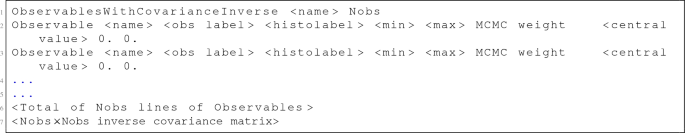
An Observable to be computed is specified in one of the following formats:
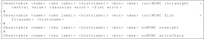
\(\texttt {<name>}\) is a user given name for different observables which must be unique for each observable.
\(\texttt {<obs label>}\) is the theory label of the observable (see the online documentation).
\(\texttt {<histolabel>}\) is used for the label of the output ROOT histogram, while \(\texttt {<min>}\) and \(\texttt {<max>}\) represent the range of the histogram (if \(\texttt {<min>}\) \(\ge \) \(\texttt {<max>}\) the range of the histogram is set automatically).
\(\texttt {(no)MCMC}\) is the flag specifying whether the observable should be included in likelihood used for the MCMC sampling.
\(\texttt {(no)weight}\) specifies if the observable weight will be computed or not. If weight is specified with noMCMC then a chain containing the weights for the observable will be stored in the MCout*.root file.
\(\texttt {noMCMC noweight}\) is the combination to be used to get a prediction for an observable.
When the weight option is specified, at least one of the \(\texttt {<Gaussian error>}\) or the \(\texttt {<flat error>} \) must be non-vanishing, and the \(\texttt {<central value>}\) must of course be specified.
When using the file option, a histogram in a ROOT file must be specified by the name of the ROOT file ( filename ) and then the name of the histogram ( histoname ) in the file (including, if needed, the directory).
The writeChain option allows one to write all the values of the observable generated during the main run of the MCMC into the ROOT file.
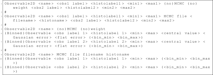
- 6.
A BinnedObservable is similar in construction to an Observable but with two extra arguments specifying the upper and lower limit of the bin:

Because of the order of parsing the \(\texttt {<central value>} \mathtt{<Gaussian error> <flat error>}\) cannot be dropped out even in the noMCMC noweight case for a BinnedObservable.
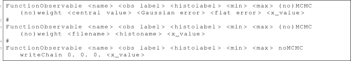
- 7.
A FunctionObservable is the same as a BinnedObservable but with only one extra argument that points to the value at which the function is computed:
- 8.
An asymmetric Gaussian constraint can be set using AsyGausObservable:

- 9.
Correlations among observables can be taken into account with the line CorrelatedGaussianObservables name Nobs, which initializes a set of Nobs correlated observables. It must be followed by exactly Nobs Observable lines and then by Nobs rows of Nobs numbers for the correlation matrix (see the above example). One can use the keywords noMCMC and noweight, instead of MCMC and weight.
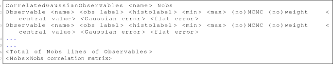
Any construction for Observable mentioned in item 5 of this list above can be used in a Correlated GaussianObservables set. Also, Binned Observables or FunctionObservables can be used instead of and alongside Observable. If noweight is specified for any Observable then that particular Observable along with the corresponding row and column of the correlation matrix is excluded from the set o CorrelatedGaussian Observables.
Correlations between any set of observables can be computed using the construction:
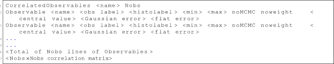
This prints the correlation matrix in the Observables/Statistics.txt file. All rules that apply to Correlated GaussianObservables also apply to CorrelatedObservables. In addition, the inverse covariance matrix of a set of Nobs Observables can be specified with the following:
- 10.
A correlation between two observables can be obtained with any of the four following specifications:
- 11.
Include configuration files with the Include File directive. This is useful if one wants to separate the input configurations for better organization and flexibility.


Step 2: Monte Carlo configuration file:
The parameters and options of the Monte Carlo run are specified in a configuration file, separate from the one(s) for the model. Each line in the file has a pair of a label and its value, separated by space(s) or tab(s). The available parameters and options are:
NChains: The number of chains in the Monte Carlo run. A minimum of 5 is suggested (default). If the theory space is complicated and/or the number of parameters is large then more chains are necessary. The amount of statistics collected in the main run is proportional to the number of chains.
PrerunMaxIter : The maximum number of iterations that the pre-run will go through (Default: 1000000). The pre-run ends automatically when the chains converge (by default R<1.1, see below) and all efficiencies are adjusted. While it is not necessary for the pre-run to converge for a run to be completed, one should exercise caution if convergence is not attained.
NIterationsUpdateMax: The maximum number of iterations after which the proposal functions are updated in the pre-run and convergence is checked. (Default: 1000)
Seed: The seed can be fixed for deterministic runs. (Default: 0, corresponding to a random seed initialization)
Iterations: The number of iterations in the main run. This run is for the purpose of collecting statistics and is at the users discretion. (Default: 100000)
MinimumEfficiency: This allows setting the minimum efficiency of all the parameters to be attained in the pre-run. (Default: 0.15)
MaximumEfficiency: This allows setting the maximum efficiency of all the parameters to be attained in the pre-run. (Default: 0.35)
RValueForConvergence: The R-value for which convergence is considered to be attained in the pre-run can be set with this flag. (Default: 1.1)
WriteParametersChains: The chains will be written in the ROOT file MCout.root. This can be used for analyzing the performance of the chains and/or to use the sampled pdf for post-processing. (Default: false)
FindModeWithMinuit: To find the global mode with MINUIT starting from the best fit parameters in the MCMC run. (Default: false)
RunMinuitOnly: To run a MINUIT minimization only, without running the MCMC. (Default: false)
CalculateNormalization: Whether the normalization of the posterior pdf will be calculated at the end of the Monte Carlo run. This is useful for model comparison. (Default: false)
NIterationNormalizationMC: The maximum number of iterations used to compute the normalization. (Default: 1000000)
PrintAllMarginalized: Whether all marginalized distributions will be printed in a pdf file (MonteCarlo_plots.pdf). (Default: true)
PrintCorrelationMatrix: Whether the parametric correlation will be printed in ParamCorrelations.pdf and ParamCorrelations.tex. (Default: false)
PrintKnowledgeUpdatePlots: Whether comparison between prior and posterior knowledge will be printed in a plot stored in ParamUpdate.pdf. (Default: false)
PrintParameterPlot: Whether a summary of the parameters will be printed in ParamSummary.pdf. (Default: false)
PrintTrianglePlot: Whether a triangle plot of the parameters will be printed. (Default: false)
WritePreRunData: Whether the pre-run data is written to a file. Useful to exploit a successful pre-run for multiple runs. (Default: false)
ReadPreRunData: Whether the pre-run data will be read from a previously stored prerun file. (Name of the file, default: empty)
MultivariateProposal: Whether the proposal function will be multivariate or uncorrelated. (Default: true)
Histogram1DSmooth: Sets the number of iterative smoothing of 1D histograms. (Default: 0)
Histogram2DType: Sets the type of 2D histograms: 1001 \(\rightarrow \) Lego (default), 101 \(\rightarrow \) Filled, 1 \(\rightarrow \) Contour.
MCMCInitialPosition: The initial distribution of chains over the parameter space. (Options: Center, RandomPrior, RandomUniform (default))
PrintLogo: Toggle the printing of the HEPfit logo on the histograms. (Default: true)
NoHistogramLegend: Toggle the printing of the histogram legend. (Default: false)
PrintLoglikelihoodPlots: Whether to print the 2D histograms for the parameters vs. loglikelihood. (Default: false)
WriteLogLikelihoodChain: Whether to write the value of log likelihood in a chain. (Default: false)
Histogram2DAlpha: Control the transparency of the 2D histograms. This does not work with all 2D histogram types. (Default: 1)
NBinsHistogram1D: The number of bins in the 1D histograms. (Default: 100, 0 sets default)
NBinsHistogram2D: The number of bins in the 2D histograms. (Default: 100, 0 sets default)
InitialPositionAttemptLimit: The maximum number of attempts made at getting a valid logarithm of the likelihood for all chains before the pre-run starts. (Default: 10000, 0 sets default)
SignificantDigits The number of significant digits appearing in the Statistics file. (Default: computed based on individual results, 0 sets default)
HistogramBufferSize: The memory allocated to each histogram. Also determines the number of events collected before setting automatically the histogram range. (Default: 100000)
For example, a Monte Carlo configuration file is written as:

where a ’#’ can be placed at the beginning of each line to comment it out.
Step 3: Run
Library mode with MCMC: An example can be found in examples/MonteCarloMode

After creating the configuration files, run with the command:

Alternative: run with MPI
HEPfit allows for parallel processing of the MCMC run and the observable computations. To allow for this HEPfit, and BAT have to be compiled with MPI support as explained in Sect. 6. The command

will launch analysis on N thread/cores/processors depending on the smallest processing unit of the hardware used. Our MPI implementation allows for runs on multi-threaded single processors as well as clusters with MPI support. Note: Our MPI implementation of HEPfit cannot be used with BAT compiled with the –enable-parallel option. It is mandatory to use the MPI patched version of BAT as explained in the online documentation.
7.2 Event generation mode
Using the model configuration file used in the Monte Carlo mode, one can obtain predictions of observables. An example can be found in examples/EventGeneration folder:

After making the configuration files, run with the command:

The \(\texttt {<number of iterations>}\) defines the number of random points in the parameter space that will be evaluated. Setting this to 0 gives the value of the observables at the central value of all the parameters. If the [output folder] is not specified everything is printed on the screen and no data is saved. Alternately, one can specify the output folder and the run will be saved if \(\texttt {<number of iterations>} \) 0. The output folder can be found in ./GeneratedEvents. The structure of the output folder is as follows.
Output folder structure:
CGO: Contains any correlated Gaussian observables that might have been listed in the model configuration files.
Observables: Contains any observables that might have been listed in the model configuration files.
Parameters: Contains all the parameters that were varied in the model configuration files.
Summary.txt: Contains a list of the model used, the parameters varied, the observables computed and the number of events generated. This can be used, for example, to access all the files from a third party program.
The parameters and the observables are stored in the respective directories in files that are named after the same. For example, the parameter lambda will be saved in the file lambda.txt in the Parameters folder.
7.3 Library mode without MCMC
The library mode allows for access to all the observables implemented in HEPfit without a Monte Carlo run. The users can specify a Model and vary ModelParameters according to their own algorithm and get the corresponding predictions for the observables. This is made possible through:
a combined library: libHEPfit.a (installed in HEPFIT_INSTALL_DIR/lib).
a combined header file: HEPfit.h (installed in HEPFIT_INSTALL_DIR/include/HEPfit).
The HEPfit library allows for two different implementations of the access algorithm.
Non-minimal mode:
In the non-minimal mode the user can use the Model conf file to pass the default value of the model parameters. The following elements must be present in the user code to define the parameters and access the observable. (For details of model parameters, observables, etc. please look up the online documentation.)

Minimal mode:
In the minimal mode the user can use the default values in the InputParameters header file to define the default values of the model parameters, therefore not requiring any additional input files to be parsed. (For details of model name, flags, parameters, observables, etc. please look up the online documentation.)


Use of hepfit-config: A hepfit-config script can be found in the HEPFIT_INSTALL_DIR/bin directory, which can be invoked with the following options:

7.4 Custom models and observables
A very useful feature of HEPfit is that it allows the user to create custom models and observables. We have already provided a template that can be found in the examples/myModel directory which can be used as a starting point. Below we describe how to implement both custom models and custom observables.
Custom models: The idea of a custom model is to define an additional set of parameters over and above what is defined in any model in HEPfit. Typically the starting point is the StandardModel, as in the template present in the HEPfit package. Going by this template in the examples/myModel directory, to create a model one has to define the following:
In the myModel.h header file:
- 1.
Define the number of additional parameters:

- 2.
Define the variables corresponding to the parameters:

- 3.
Define getters for all the parameters:

- 1.
In the myModel.cpp file:
- 1.
Define the names of the parameters (they can be different from the variable names):

- 2.
Link the parameter name to the variable containing it for all the parameters:

- 3.
Link the names of the parameters to the corresponding variables in the setParameter method:
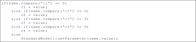
- 1.


This completes the definition of the model. One can also define flags that will control certain aspects of the model, but since this is an advanced and not so commonly used feature we will not describe it here. There is an implementation in the template for the user to follow should it be needed. Finally, the custom model needs to be added with a name to the ModelFactory in the main function as is done in examples/myModel/myModel_MCMC.cpp.

Custom observables
The definition of custom observables does not depend on having defined a custom model or not. A custom observable can be any observable that has not been defined in HEPfit. It can be a function of parameters already defined in a HEPfit model or in a custom model or a combination of the two. However, a custom observable has to be explicitly added to the ThObsFactory in the main function as is done in examples/myModel/myModel_MCMC.cpp.

The first 6 observables require an argument and hence needed boost::bind. The last two do not need an argument. The implementation of these observables can be found in examples/myModel /src/myObservables.cpp and the corresponding header file. In this template the myObservables class inherits from the THObservable class and the observables called yield, C_3 and C_4 inherit from the former. Passing an object of the StandardModel class as a reference is mandatory as is the overloading of the computeThValue method by the custom observables, which is used to compute the value of the observable at each iteration.
7.5 Example run in the Monte Carlo mode
In this section we give an example of how HEPfit can be used for a fit to data using the MCMC implementation in BAT. Once you have installed HEPfit following the instructions in Sect. 6 move to the MonteCarloMode directory and compile the code with

An example set of configuration files are packaged with the HEPfit distribution. They can be found in the examples/config directory. For convenience we will copy this directory into the MonteCarloMode directory:

The configuration files in that directory contain an example of a Unitarity triangle fit that can be done with experimental and lattice inputs. There are two files in the config directory:
StandardModel.conf: This file is the starting point of the model configurations for this example. It contains the definition of the model at the top. It then includes any other configuration files necessary for this example and a list of parameters that are mandatory for the SM implementation in HEPfit. Note that all the parameters that are mandatory for StandardModel need not be present in this file but can also be present in any other configuration file that is included with the IncludeFile directive. The StandardModel.conf file looks like

UTfit.conf: This is the second file in the config directory and included from the StandardModel.conf file. This file contains the parameters that are relevant for a Unitarity Triangle fit and a list of Observables and Observables2D that are used in the fit. There are also some ModelFlag specifications in the file which determine the model specific run configurations. More details for these can be found in the online documentation. The list of parameters looks similar to the one in StandardModel.conf

while the list of observables looks like:

There is also a MonteCarlo.conf file in the MonteCarloMode directory. This file sets all the configurations of the MCMC run and can be used for any fit after any modifications that the user might choose to make. With these files a MCMC run can be started using the command:

or

where n is the number of CPU cores the user wants to use. We ran this fit with the following modifications to the MonteCarlo.conf file

Increasing the PrerunMaxIter allows for the convergence of the chains although, in this particular run convergence occurred at under 400,000 iterations. Increasing the Iterations allows for collection of moderate amount of statistics. In this configuration using 40 CPU cores, the fit took approximately 50 minutes to complete. The output generated by the code are:

Example plots from a Unitarity Triangle fit that can be found in the MonteCarlo_plots.pdf file

Example plots from a Unitarity Triangle fit that can be found in the Observables directory
log.txt: The log file containing information on the MCMC run and is similar to the output at the terminal.
MCout.root: The ROOT file containing all the information of the run and the histograms (and possibly the corresponding chains). This file can be read and all information processed using ROOT.
MonteCarlo_results.txt: A text file containing some information on the fitted parameters. Here one can find all the details of the distributions of the parameters like the mean, standard deviation, mode and percentiles. The snippet below shows an example:
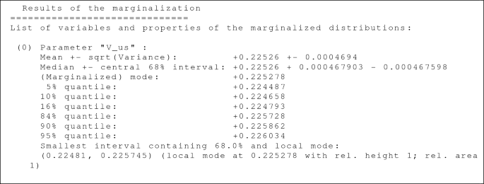
MonteCarlo_plots.pdf: A file containing the 1D and 2D histograms for the parameters. Some example 1D and 2D histograms from the Unitarity Triangle fit can be found in Fig. 6. The plots include approximate 68.3%, 95.5% and 99.7% probability regions, computed from the mode of the 1D or 2D distributions, and some statistical information.
Observables: a directory containing the histograms for all the observables specified in the configuration file, as well as some text files. Some example plots from the Unitarity Triangle fit are shown in Fig. 7.
Observables/HistoLog.txt: A file containing the information on over-run and under-run during the filling of histograms.
Observables/Statistics.txt: A file containing a compilation of the statistics extracted from the histograms of the observables. For example:
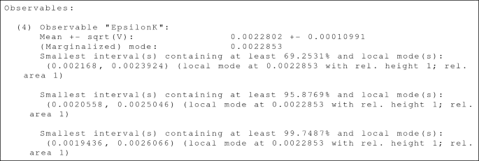
It also contains some measures that can be used for judging the goodness of fit and models comparison. For details see [6, 11, 139].
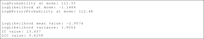


Other files might be generated depending on the options specified in the Monte Carlo configuration file.
8 Summary
HEPfit is a multipurpose and flexible analysis framework that can be used for fitting models to experimental and theoretical constraints. It comes with the ability to use the Bayesian MCMC framework implemented in BAT, which is highly efficient and allows for both factorized and non-factorized priors and is integrated with ROOT. The key features of the HEPfit framework are:
It allows for Bayesian analyses using an efficiently parallelized MCMC and for any other custom statistical analysis that the user might want to implement. This is made possible by allowing for the computation of the observables using the HEPfit library.
The Bayesian analysis framework in HEPfit using BAT is parallelized with MPI and can be run on a large number of processors without a substantial increase in the overhead. This makes the use of HEPfit extremely scalable from desktop computers to large clusters.
Over and above the models and observables defined in HEPfit, it also allows for users to define their own models and observables. This gives users the flexibility to use HEPfit for any model and set of observables of their choice. User-defined models can add new parameters and the observables can be functions of these parameters and/or of the parameters already defined in HEPfit.
HEPfit has been thoroughly tested over the years with several physics results already published. This has allowed us not only to gain confidence in the implementation of HEPfit but also to gather configuration files that are publicly available in the HEPfit repository and can be used by anyone wishing to start using HEPfit with minimal initial effort. In this article we give a summary of the structure of the code, the statistical framework used in BAT, the parallelization of the code, a brief overview of the models and observables implemented in HEPfit and an overview of the physics results that has been produced.
Eventually, this article should be also retained as an optimal starting point for installing and running HEPfit. For further technical details on the usage of HEPfit and on the structure of the code, a comprehensive online documentation is available on the HEPfit website.
Data Availability Statement
This manuscript has no associated data or the data will not be deposited. [Author’s comment: This manuscript describes a code, with no experimental data associated.]
Notes
While for a simple parameter space it is possible to compute the normalization factor, a MCMC analysis provides an unnormalized posterior distribution. This is the relevant ingredient for the purpose of studying any credibility interval. From now on, we implicitly assume we are dealing with an unnormalized posterior density.
Two CKM parameterizations (the Wolfenstein one and a parameterization using \(\vert V_{us}\vert \), \(\vert V_{cb}\vert \), \(\vert V_{ub}\vert \), and the angle \(\gamma \) of the unitarity triangle as inputs) can be selected using the model flag FlagWolfenstein.
The THDM of type II contains the scalar Higgs part of the MSSM.
The free parameters in the model also include several nuisance parameters to control theory uncertainties in certain Higgs processes.
As in the NPSMEFTd6 class, there are several nuisance parameters in the model to control theory uncertainties in certain Higgs processes. We refer to the documentation for a extensive list of the model parameters.
References
A. Caldwell, D. Kollár, K. Kröninger, BAT—the Bayesian analysis toolkit. Comput. Phys. Commun. 180, 2197–2209 (2009). arXiv:0808.2552
A.C. Caldwell, D. Kollár, K. Kröninger, BAT—the bayesian analysis toolkit. J. Phys. Conf. Ser. 219, 032013 (2010)
F. Beaujean, A. Caldwell, D. Kollár, K. Kröninger, BAT—the bayesian analysis toolkit. J. Phys. Conf. Ser. 331, 072040 (2011)
M. Ciuchini, E. Franco, S. Mishima, L. Silvestrini, Electroweak precision observables, new physics and the nature of a 126 GeV Higgs boson. JHEP 08, 106 (2013). [arXiv:1306.4644]
L. Reina, J. de Blas, M. Ciuchini, E. Franco, D. Ghosh, S. Mishima, M. Pierini, L. Silvestrini, Precision constraints on non-standard Higgs-boson couplings with HEPfit. PoS EPS–HEP2015, 187 (2015)
M. Ciuchini, M. Fedele, E. Franco, S. Mishima, A. Paul, L. Silvestrini, M. Valli, \(B\rightarrow K^* \ell ^+ \ell ^-\) decays at large recoil in the Standard Model: a theoretical reappraisal. JHEP 06, 116 (2016). arXiv:1512.07157
J. de Blas, M. Ciuchini, E. Franco, S. Mishima, M. Pierini, L. Reina, L. Silvestrini, Electroweak precision observables and Higgs-boson signal strengths in the Standard Model and beyond: present and future. JHEP 12, 135 (2016). [arXiv:1608.01509]
V. Cacchio, D. Chowdhury, O. Eberhardt, C.W. Murphy, Next-to-leading order unitarity fits in two-Higgs-doublet models with soft \({\mathbb{Z}}_2\) breaking. JHEP 11, 026 (2016). arXiv:1609.01290
M. Ciuchini, M. Fedele, E. Franco, S. Mishima, A. Paul, L. Silvestrini, M. Valli, \(B\rightarrow K^*\ell ^+\ell ^-\) in the Standard Model: elaborations and Interpretations. PoS ICHEP2016, 584 (2016). arXiv:1611.04338
J. de Blas, M. Ciuchini, E. Franco, S. Mishima, M. Pierini, L. Reina, L. Silvestrini, Electroweak precision constraints at present and future colliders. PoS ICHEP2016, 690 (2017). arXiv:1611.05354
M. Ciuchini, A.M. Coutinho, M. Fedele, E. Franco, A. Paul, L. Silvestrini, M. Valli, On flavourful easter eggs for new physics hunger and lepton flavour universality violation. Eur. Phys. J. C 77(10), 688 (2017). arXiv:1704.05447
M. Ciuchini, M. Fedele, E. Franco, S. Mishima, A. Paul, L. Silvestrini, M. Valli, Knowns and unknowns in the predictions for \(B \rightarrow K^{*}\mu ^{+}\mu ^{-}\). Nucl. Part. Phys. Proc. 285–286, 45–49 (2017)
O. Eberhardt, Two-Higgs-doublet model fits with HEPfit, in Proceedings, 2017 European Physical Society Conference on High Energy Physics (EPS-HEP 2017): Venice, Italy, July 5-12, 2017, (2017). arXiv:1709.09414
S. Gori, C. Grojean, A. Juste, A. Paul, Heavy Higgs searches: flavour matters. JHEP 01, 108 (2018). arXiv:1710.03752
J. de Blas, M. Ciuchini, E. Franco, S. Mishima, M. Pierini, L. Reina, L. Silvestrini, The global electroweak and Higgs fits in the LHC era. PoS EPS–HEP2017, 467 (2017). arXiv:1710.05402
D. Chowdhury, O. Eberhardt, Update of global two-Higgs-doublet model fits. JHEP 05, 161 (2018). arXiv:1711.02095
J. de Blas, O. Eberhardt, C. Krause, Current and future constraints on Higgs couplings in the nonlinear effective theory. JHEP 07, 048 (2018). arXiv:1803.00939
C.-W. Chiang, G. Cottin, O. Eberhardt, Global fits in the Georgi-Machacek model. Phys. Rev. D 99(1), 015001 (2019). arXiv:1807.10660
L. Cheng, O. Eberhardt, C.W. Murphy, Novel theoretical constraints for color-octet scalar models. Chin. Phys. C 43(9), 093101 (2019). arXiv:1808.05824
O. Eberhardt, Current status of two-Higgs-doublet models with a softly broken \({\mathbb{Z}}_2\) symmetry, in 39th International Conference on High Energy Physics (ICHEP 2018) Seoul, Gangnam-Gu, Republic of Korea, July 4–11, 2018 (2018). arXiv:1809.04851
M. Ciuchini, A.M. Coutinho, M. Fedele, E. Franco, A. Paul, L. Silvestrini, M. Valli, Hadronic uncertainties in the \(B\rightarrow K^*\mu ^+\mu ^-\) decay. PoS BEAUTY2018, 044 (2018). arXiv:1809.03789
M. Ciuchini, A.M. Coutinho, M. Fedele, E. Franco, A. Paul, L. Silvestrini, M. Valli, On hadronic uncertainties polluting the New Physics hunt in \(b \rightarrow s\) transitions. Nucl. Part. Phys. Proc. 303–305, 8–13 (2018)
F. Buccella, A. Paul, P. Santorelli, \(SU(3)_F\) breaking through final state interactions and \(CP\) asymmetries in \(D \rightarrow PP\) decays. Phys. Rev. D 99(11), 113001 (2019). arXiv:1902.05564
M. Ciuchini, A.M. Coutinho, M. Fedele, E. Franco, A. Paul, L. Silvestrini, M. Valli, New Physics in \(b \rightarrow s \ell ^+ \ell ^-\) confronts new data on lepton universality. Eur. Phys. J. C 79(8), 719 (2019). arXiv:1903.09632
P. Arnan, A. Crivellin, M. Fedele, F. Mescia, Generic loop effects of new scalars and fermions in \(b\rightarrow s\ell ^+\ell ^-\) and a vector-like \(4^{\rm th}\) generation. JHEP 06, 118 (2019). arXiv:1904.05890
D. Bečirević, M. Fedele, I. Nišandžić, A. Tayduganov, Lepton flavor universality tests through angular observables of \(\overline{B}\rightarrow D^{(\ast )}\ell \overline{\nu }\) decay modes. arXiv:1907.02257
J. de Blas et al., Higgs boson studies at future particle colliders. JHEP 01, 139 (2020). arXiv:1905.03764
J. de Blas, G. Durieux, C. Grojean, J. Gu, A. Paul, On the future of Higgs, electroweak and diboson measurements at lepton colliders. JHEP 12, 117 (2019). arXiv:1907.04311
G. Durieux, A. Irles, V. Miralles, A. Peñuelas, R. Pöschl, M. Perelló, M. Vos, The electro-weak couplings of the top and bottom quarks - global fit and future prospects. JHEP 12, 098 (2019). arXiv:1907.10619
L. Darmé, M. Fedele, K. Kowalska, E.M. Sessolo, Flavour anomalies from a split dark sector, arXiv:2002.11150
HEPfit Collaboration. https://hepfit.roma1.infn.it
A. Gelman, D.B. Rubin, Inference from iterative simulation using multiple sequences. Stat. Sci. 7(4), 457–472 (1992)
S.P. Brooks, A. Gelman, General methods for monitoring convergence of iterative simulations. J. Comput. Graph. Stat. 7(4), 434–455 (1998). https://www.tandfonline.com/doi/pdf/10.1080/10618600.1998.10474787
T. Lee, A theory of spontaneous T violation. Phys. Rev. D 8, 1226–1239 (1973)
J.F. Gunion, H.E. Haber, The CP conserving two Higgs doublet model: the approach to the decoupling limit. Phys. Rev. D 67, 075019 (2003). arXiv:hep-ph/0207010
G. Branco, P. Ferreira, L. Lavoura, M. Rebelo, M. Sher et al., Theory and phenomenology of two-Higgs-doublet models. Phys. Rep. 516, 1–102 (2012). arXiv:1106.0034
D. Chowdhury, O. Eberhardt, Global fits of the two-loop renormalized two-Higgs-doublet model with soft Z\(_{2}\) breaking. JHEP 11, 052 (2015). arXiv:1503.08216
A.I. Bochkarev, S.V. Kuzmin, M.E. Shaposhnikov, Electroweak baryogenesis and the Higgs boson mass problem. Phys. Lett. B 244, 275–278 (1990)
A.E. Nelson, D.B. Kaplan, A.G. Cohen, Why there is something rather than nothing: matter from weak interactions. Nucl. Phys. B 373, 453–478 (1992)
G.C. Dorsch, S.J. Huber, J.M. No, A strong electroweak phase transition in the 2HDM after LHC8. JHEP 10, 029 (2013). arXiv:1305.6610
H. Georgi, M. Machacek, Doubly charged Higgs bosons. Nucl. Phys. B 262, 463–477 (1985)
M.S. Chanowitz, M. Golden, Higgs boson triplets with \(M_W=M_Z \cos \theta _W\). Phys. Lett. 165B, 105–108 (1985)
G. Altarelli, R. Barbieri, Vacuum polarization effects of new physics on electroweak processes. Phys. Lett. B 253, 161–167 (1991)
G. Altarelli, R. Barbieri, S. Jadach, Toward a model independent analysis of electroweak data. Nucl. Phys. B 369, 3–32 (1992)
G. Altarelli, R. Barbieri, S. Jadach, Toward a model independent analysis of electroweak data. Nucl. Phys. B 376, 444 (1992)
G. Altarelli, R. Barbieri, F. Caravaglios, Nonstandard analysis of electroweak precision data. Nucl. Phys. B 405, 3–23 (1993)
M.E. Peskin, T. Takeuchi, Estimation of oblique electroweak corrections. Phys. Rev. D 46, 381–409 (1992)
R. Barbieri, A. Pomarol, R. Rattazzi, A. Strumia, Electroweak symmetry breaking after LEP1 and LEP2. Nucl. Phys. B 703, 127–146 (2004). arXiv:hep-ph/0405040
F. del Aguila, M. Pérez-Victoria, J. Santiago, Observable contributions of new exotic quarks to quark mixing. JHEP 09, 011 (2000). arXiv:hep-ph/0007316
F. del Aguila, J. de Blas, M. Pérez-Victoria, Effects of new leptons in electroweak precision data. Phys. Rev. D 78, 013010 (2008). arXiv:0803.4008
F. del Aguila, J. de Blas, M. Pérez-Victoria, Electroweak limits on general new vector bosons. JHEP 09, 033 (2010). arXiv:1005.3998
J. de Blas, M. Chala, M. Pérez-Victoria, J. Santiago, Observable effects of general new scalar particles. JHEP 04, 078 (2015). arXiv:1412.8480
A. Drozd, J. Ellis, J. Quevillon, T. You, The universal one-loop effective action. JHEP 03, 180 (2016). arXiv:1512.03003
F. del Aguila, Z. Kunszt, J. Santiago, One-loop effective lagrangians after matching. Eur. Phys. J. C 76(5), 244 (2016). arXiv:1602.00126
B. Henning, X. Lu, H. Murayama, One-loop matching and running with covariant derivative expansion. JHEP 01, 123 (2018). arXiv:1604.01019
S.A.R. Ellis, J. Quevillon, T. You, Z. Zhang, Mixed heavy-light matching in the universal one-loop effective action. Phys. Lett. B 762, 166–176 (2016). arXiv:1604.02445
J. Fuentes-Martin, J. Portoles, P. Ruiz-Femenia, Integrating out heavy particles with functional methods: a simplified framework. JHEP 09, 156 (2016). arXiv:1607.02142
Z. Zhang, Covariant diagrams for one-loop matching. JHEP 05, 152 (2017). arXiv:1610.00710
S.A.R. Ellis, J. Quevillon, T. You, Z. Zhang, Extending the universal one-loop effective action: heavy-light coefficients. JHEP 08, 054 (2017). arXiv:1706.07765
J.D. Wells, Z. Zhang, Effective field theory approach to trans-TeV supersymmetry: covariant matching. Yukawa unification and Higgs couplings. JHEP 05, 182 (2018). arXiv:1711.04774
J. de Blas, J.C. Criado, M. Perez-Victoria, J. Santiago, Effective description of general extensions of the Standard Model: the complete tree-level dictionary. JHEP 03, 109 (2018). arXiv:1711.10391
B. Grzadkowski, M. Iskrzynski, M. Misiak, J. Rosiek, Dimension-six terms in the Standard Model Lagrangian. JHEP 10, 085 (2010). arXiv:1008.4884
R. Contino, C. Grojean, M. Moretti, F. Piccinini, R. Rattazzi, Strong double Higgs production at the LHC. JHEP 1005, 089 (2010). arXiv:1002.1011
A. Azatov, R. Contino, J. Galloway, Model-independent bounds on a light Higgs. JHEP 1204, 127 (2012). arXiv:1202.3415
LHC Higgs Cross Section Working Group Collaboration, A. David, A. Denner, M. Duehrssen, M. Grazzini, C. Grojean, G. Passarino, M. Schumacher, M. Spira, G. Weiglein, M. Zanetti, LHC HXSWG interim recommendations to explore the coupling structure of a Higgs-like particle, arXiv:1209.0040
A. Sirlin, Radiative corrections in the \(SU(2)_L\times U(1)\) theory: A simple renormalization framework. Phys. Rev. D 22, 971–981 (1980)
W. Marciano, A. Sirlin, Radiative corrections to neutrino induced neutral current phenomena in the \(SU(2)_L\times U(1)\) theory. Phys. Rev. D 22, 2695 (1980)
W. Marciano, A. Sirlin, Radiative corrections to neutrino induced neutral current phenomena in the \(SU(2)_L\times U(1)\) theory. Phys. Rev. D 31, 213 (1985)
A. Djouadi, C. Verzegnassi, Virtual very heavy top effects in LEP/SLC precision measurements. Phys. Lett. B 195, 265 (1987)
A. Djouadi, \({{\cal{O}}}(\alpha \alpha _s)\) vacuum polarization functions of the standard model gauge bosons. Nuovo Cim. A 100, 357 (1988)
B.A. Kniehl, Two-loop corrections to the vacuum polarizations in perturbative QCD. Nucl. Phys. B 347, 86–104 (1990)
F. Halzen, B.A. Kniehl, \(\Delta r\) beyond one loop. Nucl. Phys. B 353, 567–590 (1991)
B.A. Kniehl, A. Sirlin, Dispersion relations for vacuum polarization functions in electroweak physics. Nucl. Phys. B 371, 141–148 (1992)
B.A. Kniehl, A. Sirlin, On the effect of the \(t \bar{t}\) threshold on electroweak parameters. Phys. Rev. D 47, 883–893 (1993)
R. Barbieri, M. Beccaria, P. Ciafaloni, G. Curci, A. Vicere, Radiative correction effects of a very heavy top. Phys. Lett. B 288, 95–98 (1992). arXiv:hep-ph/9205238
R. Barbieri, M. Beccaria, P. Ciafaloni, G. Curci, A. Vicere, Two-loop heavy top effects in the standard model. Nucl. Phys. B 409, 105–127 (1993)
A. Djouadi, P. Gambino, Electroweak gauge bosons selfenergies: Complete QCD corrections. Phys. Rev. D 49, 3499–3511 (1994)
A. Djouadi, P. Gambino, Electroweak gauge bosons selfenergies: Complete QCD corrections. Phys. Rev. D 53, 4111 (1996). [hep-ph/9309298]
J. Fleischer, O. Tarasov, F. Jegerlehner, Two-loop heavy top corrections to the \(\rho \) parameter: A simple formula valid for arbitrary Higgs mass. Phys. Lett. B 319, 249–256 (1993)
J. Fleischer, O. Tarasov, F. Jegerlehner, Two-loop large top mass corrections to electroweak parameters: Analytic results valid for arbitrary Higgs mass. Phys. Rev. D 51, 3820–3837 (1995)
L. Avdeev, J. Fleischer, S. Mikhailov, O. Tarasov, \({\cal{O}}(\alpha \alpha _s^2)\) correction to the electroweak \(\rho \) parameter. Phys. Lett. B 336, 560–566 (1994)
L. Avdeev, J. Fleischer, S. Mikhailov, O. Tarasov, \({\cal{O}}(\alpha \alpha _s^2)\) correction to the electroweak \(\rho \) parameter. Phys. Lett. B 349, 597–598 (1995). [hep-ph/9406363]
K. Chetyrkin, J.H. Kuhn, M. Steinhauser, Corrections of order \({\cal{O}}(G_F M_t^2 \alpha _s^2)\) to the \(\rho \) parameter. Phys. Lett. B 351, 331–338 (1995). arXiv:hep-ph/9502291
K. Chetyrkin, J.H. Kuhn, M. Steinhauser, QCD corrections from top quark to relations between electroweak parameters to order \(\alpha _s^2\). Phys. Rev. Lett. 75, 3394–3397 (1995). arXiv:hep-ph/9504413
G. Degrassi, P. Gambino, A. Vicini, Two-loop heavy top effects on the \(m_Z\)-\(m_W\) interdependence. Phys. Lett. B 383, 219–226 (1996). arXiv:hep-ph/9603374
G. Degrassi, P. Gambino, A. Sirlin, Precise calculation of \(M_W\), \(\sin ^2{\hat{\theta }}_W(M_Z)\), and \(\sin ^2\theta _{{\rm eff}}^{{\rm lept}}\). Phys. Lett. B 394, 188–194 (1997). arXiv:hep-ph/9611363
G. Degrassi, P. Gambino, Two-loop heavy top corrections to the \(Z^0\) boson partial widths. Nucl. Phys. B 567, 3–31 (2000). arXiv:hep-ph/9905472
A. Freitas, W. Hollik, W. Walter, G. Weiglein, Complete fermionic two-loop results for the \(M_W\)-\(M_Z\) interdependence. Phys. Lett. B 495, 338–346 (2000)
A. Freitas, W. Hollik, W. Walter, G. Weiglein, Complete fermionic two-loop results for the \(M_W\)-\(M_Z\) interdependence. Phys. Lett. B 570, 260–264 (2003). arXiv:hep-ph/0007091
J. van der Bij, K. Chetyrkin, M. Faisst, G. Jikia, T. Seidensticker, Three-loop leading top mass contributions to the \(\rho \) parameter. Phys. Lett. B 498, 156–162 (2001). arXiv:hep-ph/0011373
A. Freitas, W. Hollik, W. Walter, G. Weiglein, Electroweak two-loop corrections to the \(M_W\)-\(M_Z\) mass correlation in the standard model. Nucl. Phys. B 632, 189–218 (2002)
A. Freitas, W. Hollik, W. Walter, G. Weiglein, Electroweak two-loop corrections to the \(M_W\)-\(M_Z\) mass correlation in the standard model. Nucl. Phys. B 666, 305–307 (2003). arXiv:hep-ph/0202131
M. Awramik, M. Czakon, Complete two loop bosonic contributions to the muon lifetime in the standard model. Phys. Rev. Lett. 89, 241801 (2002). arXiv:hep-ph/0208113
A. Onishchenko, O. Veretin, Two-loop bosonic electroweak corrections to the muon lifetime and \(M_Z\)-\(M_W\) interdependence. Phys. Lett. B 551, 111–114 (2003). [hep-ph/0209010]
M. Awramik, M. Czakon, A. Onishchenko, O. Veretin, Bosonic corrections to \(\Delta r\) at the two loop level. Phys. Rev. D 68, 053004 (2003). arXiv:hep-ph/0209084
M. Awramik, M. Czakon, Two loop electroweak bosonic corrections to the muon decay lifetime. Nucl. Phys. Proc. Suppl. 116, 238–242 (2003). arXiv:hep-ph/0211041
M. Awramik, M. Czakon, Complete two loop electroweak contributions to the muon lifetime in the standard model. Phys. Lett. B 568, 48–54 (2003). arXiv:hep-ph/0305248
M. Awramik, M. Czakon, A. Freitas, G. Weiglein, Precise prediction for the \(W\) boson mass in the standard model. Phys. Rev. D 69, 053006 (2004). arXiv:hep-ph/0311148
M. Faisst, J.H. Kuhn, T. Seidensticker, O. Veretin, Three loop top quark contributions to the rho parameter. Nucl. Phys. B 665, 649–662 (2003). arXiv:hep-ph/0302275
I. Dubovyk, A. Freitas, J. Gluza, T. Riemann, J. Usovitsch, The two-loop electroweak bosonic corrections to \(\sin ^2\theta ^{{\rm b}} _{{\rm eff}}\). Phys. Lett. B 762, 184–189 (2016). arXiv:1607.08375
I. Dubovyk, A. Freitas, J. Gluza, T. Riemann, J. Usovitsch, Complete electroweak two-loop corrections to Z boson production and decay. Phys. Lett. B 783, 86–94 (2018). arXiv:1804.10236
D. Kennedy, B. Lynn, Electroweak radiative corrections with an effective Lagrangian: four fermion processes. Nucl. Phys. B 322, 1–54 (1989)
D. Kennedy, B. Lynn, C. Im, R. Stuart, Electroweak cross-sections and asymmetries at the \(Z^0\). Nucl. Phys. B 321, 83 (1989)
M.E. Peskin, T. Takeuchi, A new constraint on a strongly interacting Higgs sector. Phys. Rev. Lett. 65, 964–967 (1990)
P. Bamert, C. Burgess, J.M. Cline, D. London, E. Nardi, \(R_b\) and new physics: a comprehensive analysis. Phys. Rev. D 54, 4275–4300 (1996). arXiv:hep-ph/9602438
H.E. Haber, H.E. Logan, Radiative corrections to the \(Zb\bar{b}\) vertex and constraints on extended Higgs sectors. Phys. Rev. D 62, 015011 (2000). arXiv:hep-ph/9909335
D. Choudhury, T.M. Tait, C. Wagner, Beautiful mirrors and precision electroweak data. Phys. Rev. D 65, 053002 (2002). arXiv:hep-ph/0109097
K. Agashe, R. Contino, L. Da Rold, A. Pomarol, A custodial symmetry for \(Zb\bar{b}\). Phys. Lett. B 641, 62–66 (2006). arXiv:hep-ph/0605341
A. Djouadi, G. Moreau, F. Richard, Resolving the A\(_{{\rm FB}}^{{\rm b}}\) puzzle in an extra dimensional model with an extended gauge structure. Nucl. Phys. B 773, 43–64 (2007). arXiv:hep-ph/0610173
K. Kumar, W. Shepherd, T.M. Tait, R. Vega-Morales, Beautiful mirrors at the LHC. JHEP 1008, 052 (2010). arXiv:1004.4895
L. Da Rold, Solving the \(A_{FB}^b\) anomaly in natural composite models. JHEP 1102, 034 (2011). arXiv:1009.2392
E. Alvarez, L. Da Rold, A. Szynkman, A composite Higgs model analysis of forward-backward asymmetries in the production of tops at Tevatron and bottoms at LEP and SLC. JHEP 1105, 070 (2011). arXiv:1011.6557
R. Dermisek, S.-G. Kim, A. Raval, New vector boson near the Z-pole and the puzzle in precision electroweak data. Phys. Rev. D 84, 035006 (2011). arXiv:1105.0773
A. Djouadi, G. Moreau, F. Richard, Forward-backward asymmetries of the bottom and top quarks in warped extra-dimensional models: LHC predictions from the LEP and Tevatron anomalies. Phys. Lett. B 701, 458–464 (2011). arXiv:1105.3158
R. Dermisek, S.-G. Kim, A. Raval, Z’ near the Z-pole. Phys. Rev. D 85, 075022 (2012). arXiv:1201.0315
B. Batell, S. Gori, L.-T. Wang, Higgs couplings and precision electroweak data. JHEP 1301, 139 (2013). arXiv:1209.6382
D. Guadagnoli, G. Isidori, \(B(B_s \rightarrow \mu ^{+} \mu ^{-})\) as an electroweak precision test. Phys. Lett. B 724, 63–67 (2013). arXiv:1302.3909
W. Buchmuller, D. Wyler, Effective Lagrangian analysis of new interactions and flavor conservation. Nucl. Phys. B 268, 621 (1986)
Belle II Collaboration, E. Kou et al., The Belle II Physics Book , arXiv:1808.10567
S. Descotes-Genon, A. Falkowski, M. Fedele, M. González-Alonso, J. Virto, The CKM parameters in the SMEFT. JHEP 05, 172 (2019). arXiv:1812.08163
L. Silvestrini, M. Valli, Model-independent bounds on the standard model effective theory from flavour physics, arXiv:1812.10913
N.G. Deshpande, E. Ma, Pattern of symmetry breaking with two Higgs doublets. Phys. Rev. D 18, 2574 (1978)
I.F. Ginzburg, I.P. Ivanov, Tree-level unitarity constraints in the most general 2HDM. Phys. Rev. D 72, 115010 (2005). arXiv:hep-ph/0508020
B. Grinstein, C.W. Murphy, P. Uttayarat, One-loop corrections to the perturbative unitarity bounds in the CP-conserving two-Higgs doublet model with a softly broken \( {{mathbb Z}}_2 \) symmetry. JHEP 06, 070 (2016). arXiv:1512.04567
A. Barroso, P.M. Ferreira, I.P. Ivanov, R. Santos, Metastability bounds on the two Higgs doublet model. JHEP 06, 045 (2013). arXiv:1303.5098
A. Arhrib, R. Benbrik, M. Chabab, G. Moultaka, M.C. Peyranere, L. Rahili, J. Ramadan, The Higgs potential in the type II seesaw model. Phys. Rev. D 84, 095005 (2011). arXiv:1105.1925
M. Aoki, S. Kanemura, Unitarity bounds in the Higgs model including triplet fields with custodial symmetry. Phys. Rev. D 77(9), 095009 (2008). arXiv:0712.4053 (erratum: Phys. Rev. D 89(5), 059902, 2014)
R.K. Ellis et al., Physics Briefing Book, arXiv:1910.11775
HL-LHC, HE-LHC Working Group Collaboration, P. Azzi et al., Standard Model Physics at the HL-LHC and HE-LHC, arXiv:1902.04070
HL/HE WG2 group Collaboration, M. Cepeda et al., Higgs Physics at the HL-LHC and HE-LHC, arXiv:1902.00134
FCC Collaboration, A. Abada et al., FCC-ee: the lepton collider. Eur. Phys. J. ST 228(2), 261–623 (2019)
FCC Collaboration, A. Abada et al., FCC Physics Opportunities. Eur. Phys. J. C 79(6), 474 (2019)
A. Khodjamirian, T. Mannel, A.A. Pivovarov, Y.M. Wang, Charm-loop effect in \(B \rightarrow K^{(*)} \ell ^{+} \ell ^{-}\) and \(B\rightarrow K^*\gamma \). JHEP 09, 089 (2010). arXiv:1006.4945
LHCb Collaboration, R. Aaij et al., Test of lepton universality with \(B^{0} \rightarrow K^{*0}\ell ^{+}\ell ^{-}\) decays. JHEP 08, 055 (2017). arXiv:1705.05802
LHCb Collaboration, R. Aaij et al., Observation of CP violation in charm decays. Phys. Rev. Lett. 122(21), 211803 (2019). arXiv:1903.08726
LHCb Collaboration, F. Betti, Observation of CP violation in charm decays at LHCb, in 54th Rencontres de Moriond on Electroweak Interactions and Unified Theories (Moriond EW 2019) La Thuile, Italy, March 16–23, 2019 (2019). arXiv:1905.05428
LHCb Collaboration, T. Pajero, Measurements of time-dependent \(C\!P\) violation and mixing in charm at LHCb, in 17th Conference on Flavor Physics and CP Violation (FPCP 2019) Victoria, BC, Canada, May 6–10, 2019 (2019). arXiv:1907.01292
C.W. Murphy, NLO perturbativity bounds on quartic couplings in renormalizable theories with \(\phi ^4\)-like scalar sectors. Phys. Rev. D 96(3), 036006 (2017). arXiv:1702.08511
T. Ando, Predictive bayesian model selection. Am. J. Math. Manag. Sci. 31(1–2), 13–38 (2011). https://doi.org/10.1080/01966324.2011.10737798
D. M. Straub, flavio: a python package for flavour and precision phenomenology in the standard model and beyond, arXiv:1810.08132
S. Heinemeyer, W. Hollik, G. Weiglein, FeynHiggs: a program for the calculation of the masses of the neutral CP even Higgs bosons in the MSSM. Comput. Phys. Commun. 124, 76–89 (2000). arXiv:hep-ph/9812320
H. Bahl, T. Hahn, S. Heinemeyer, W. Hollik, S. Paßehr, H. Rzehak, G. Weiglein, Precision calculations in the MSSM Higgs-boson sector with FeynHiggs 2.14. arXiv:1811.09073
F. Mahmoudi, SuperIso v2.3: a program for calculating flavor physics observables in supersymmetry. Comput. Phys. Commun. 180, 1579–1613 (2009). arXiv:0808.3144
D. Chowdhury, R. Garani, S.K. Vempati, SUSEFLAV: Program for supersymmetric mass spectra with seesaw mechanism and rare lepton flavor violating decays. Comput. Phys. Commun. 184, 899–918 (2013). [arXiv:1109.3551]
H. Flacher, M. Goebel, J. Haller, A. Hocker, K. Monig et al., Revisiting the global electroweak fit of the standard model and beyond with Gfitter. Eur. Phys. J. C 60, 543–583 (2009). arXiv:0811.0009
F. Herren, M. Steinhauser, Version 3 of RunDec and CRunDec. Comput. Phys. Commun. 224, 333–345 (2018). arXiv:1703.03751
A. Akhundov, A. Arbuzov, S. Riemann, T. Riemann, The ZFITTER project. Phys. Part. Nucl. 45(3), 529–549 (2014). arXiv:1302.1395
J. Alwall, R. Frederix, S. Frixione, V. Hirschi, F. Maltoni, O. Mattelaer, H.S. Shao, T. Stelzer, P. Torrielli, M. Zaro, The automated computation of tree-level and next-to-leading order differential cross sections, and their matching to parton shower simulations. JHEP 07, 079 (2014). arXiv:1405.0301
Acknowledgements
The HEPfit developers would like to thank several physicists who have contributed indirectly to its development with suggestions, bug reporting and usage of the code. The developers would also like to thank the authors of flavio [140], in particular David Straub, since a large fraction of the flavour physics code in HEPfit has been tested against it. At various stages of its development, we have compared HEPfit with other publicly available codes, namely, FeynHiggs [141, 142], SuperISO [143], SuSeFLAV [144], Gfitter [145], RunDec [146], and ZFITTER [147]. The developers also acknowledge the use of Madgraph [148] and its allied frameworks. L.R. has been supported by the U.S. Department of Energy under grant DE-SC0010102. D.C. has been supported by the (Indo-French) CEFIPRA/IFCPAR Project No. 5404-2. Several of the developers of HEPfit were supported by the European Research Council under the European Union’s Seventh Framework Programme (FP/2007-2013)/ERC Grant Agreement n. 279972 “NPFlavour”. This project has received funding from the European Research Council (ERC) under the European Union’s Horizon 2020 research and innovation program (grant agreement no. 772369). M.C. is associated to the Dipartimento di Matematica e Fisica, Università di Roma Tre, and E.F. and L.S. are associated to the Dipartimento di Fisica, Università di Roma “La Sapienza”. V.M. and A.Pe. are supported by the Spanish Government and ERDF funds from the EU Commission [Grant FPA2017-84445-P], the Generalitat Valenciana [Grant Prometeo/2017/053], the Spanish Centro de Excelencia Severo Ochoa Programme [Grant SEV-2014-0398] and funded by Ministerio de Ciencia, Innovación y Universidades, Spain [Grant FPU16/01911] and [Grant FPU15/05103] respectively. M.F. acknowledge the financial support from MINECO grant FPA2016- 76005-C2-1-P, Maria de Maetzu program grant MDM-2014-0367 of ICCUB and 2017 SGR 929. G.G.d.C. is supported by the National Science Centre, Poland, under research grant no. 2017/26/D/ST2/00225. The work of S.M. has been supported by JSPS KAKENHI Grant No. 17K05429. M.V. is supported by the NSF Grant No. PHY-1915005. N.Y. is supported by JSPS KAKENHI Grant Numbers JP15H05889, JP15K21733, and JP17H02875. A.M.C. acknowledges support by the Swiss National Science Foundation (SNF) under contract 200021_178967. We would also like to thank the developers of BAT, in particular F. Beaujean, K. Kröninger and D. Greenwald for support during various stages of integration of BAT with HEPfit.
Author information
Authors and Affiliations
Corresponding author
Rights and permissions
Open Access This article is licensed under a Creative Commons Attribution 4.0 International License, which permits use, sharing, adaptation, distribution and reproduction in any medium or format, as long as you give appropriate credit to the original author(s) and the source, provide a link to the Creative Commons licence, and indicate if changes were made. The images or other third party material in this article are included in the article’s Creative Commons licence, unless indicated otherwise in a credit line to the material. If material is not included in the article’s Creative Commons licence and your intended use is not permitted by statutory regulation or exceeds the permitted use, you will need to obtain permission directly from the copyright holder. To view a copy of this licence, visit http://creativecommons.org/licenses/by/4.0/.
Funded by SCOAP3
About this article

Cite this article
de Blas, J., Chowdhury, D., Ciuchini, M. et al. HEPfit: a code for the combination of indirect and direct constraints on high energy physics models. Eur. Phys. J. C 80, 456 (2020). https://doi.org/10.1140/epjc/s10052-020-7904-z
Received:
Accepted:
Published:
DOI: https://doi.org/10.1140/epjc/s10052-020-7904-z