Modelling Offset Regions around Static and Mobile Locations on a Discrete Global Grid System: An IoT Case Study


People in Motion Lab, Department of Geodesy and Geomatics Engineering, University of New Brunswick, Fredericton, NB E3B 5A3, Canada
*
Author to whom correspondence should be addressed.
ISPRS Int. J. Geo-Inf. 2020, 9(5), 335; https://doi.org/10.3390/ijgi9050335
Submission received: 23 March 2020
/
Revised: 4 May 2020
/
Accepted: 15 May 2020
/
Published: 20 May 2020
(This article belongs to the Special Issue Global Grid Systems)
Abstract
:With the huge volume of location-based point data being generated by Internet of Things (IoT) devices and subsequent rising interest from the Digital Earth community, a need has emerged for spatial operations that are compatible with Digital Earth frameworks, the foundation of which are Discrete Global Grid Systems (DGGSs). Offsetting is a fundamental spatial operation that allows us to determine the region within a given distance of an IoT device location, which is important for visualizing or querying nearby location-based data. Thus, in this paper, we present methods of modelling an offset region around the point location of an IoT device (both static and mobile) that is quantized into a cell of a DGGS. Notably, these methods illustrate how the underlying indexing structure of a DGGS can be utilized to determine the cells in an offset region at different spatial resolutions. For a static IoT device location, we describe a single resolution approach as well as a multiresolution approach that allows us to efficiently determine the cells in an offset region at finer (or coarser) resolutions. For mobile IoT device locations, we describe methods to efficiently determine the cells in successive offset regions at fine and coarse resolutions. Lastly, we present a variety of results that demonstrate the effectiveness of the proposed methods.
1. Introduction
The Internet of Things (IoT) consists of millions of devices that are generating a massive amount of location-based point data on a global scale. The rapid development of location-enabled IoT devices (such as sensors, smartphones, and vehicles) has led to their adoption in a wide variety of application domains such as smart cities, transportation, energy, and agriculture, in order to better understand spatial patterns and to derive insights from a spatial perspective. As [1] points out, all IoT devices are located somewhere in space and spatial relationships exist between them, which makes location an essential component of IoT data. This has prompted researchers to design an IoT-GIS platform [2], investigate the potential of using IoT data for geospatial analysis [3], study location privacy for IoT services and applications [4], and propose the Internet of Spatial Things [5].
Owing to the volume, variety, and global scope of location-based point data being generated by IoT devices, interest from the Digital Earth community is growing. In [6] the authors summarize the evolving relationship between Digital Earth and the IoT by exploring the frictions and synergies in creating a combined IoT-Digital Earth infrastructure. Digital Earths use a three-dimensional model of the Earth’s surface to reference geospatial data (be it raster or vector data) because it provides a more realistic representation that avoids many issues associated with a two-dimensional map projection (e.g., polar singularities and map distortions). Notably, the foundation of modern Digital Earth frameworks are Discrete Global Grid Systems (DGGSs) [7,8].
DGGSs represent a class of spatial data structures that consist of a hierarchy of global grids at multiple resolutions, whereby each grid is a discretization of the Earth’s surface into a uniform arrangement of cells [9]. A DGGS is typically created by partitioning the faces of a platonic solid into equal area cells (triangles, quadrilaterals, or hexagons), and then inversely projecting those cells onto the surface of the sphere or ellipsoid using an equal area projection [10]. This approach was adopted by the Open Geospatial Consortium (OGC) in 2017 as the basis for the DGGS Abstract Specification [11] which aims to standardize the DGGS model. Importantly, DGGSs adopt an indexing method to ensure each cell has a unique index or identifier (ID) which is subsequently used to reference geospatial data [12]. Moreover, a cell ID can encode both position and spatial resolution which allows a cell to be used to represent a vector point, raster pixel, or data bucket. As a result, DGGSs enable big geospatial data to be stored, integrated, and managed at different spatial resolutions in a common, global, scalable, hierarchical framework [13,14,15,16].
From an IoT perspective, it is especially beneficial to use a cell as a data bucket to efficiently index and aggregate huge volumes of point data stemming from IoT devices because it facilitates summarization, analysis, and visualisation at varying spatial resolutions, which researchers have already started to explore with respect to crowdsensing data [17] and ride-sharing data [18]. We can also use a cell to represent the point location of a single IoT device. In fact, according to [19], the optimal solution for representing point location in a Digital Earth framework is actually based on DGGS cells and their corresponding IDs, not tuples of real numbers (i.e., latitude-longitude coordinates). Consequently, to exploit IoT data that is embedded in a Digital Earth, a need has emerged for spatial operations that are compatible with the underlying DGGS framework.
Offsetting, also known as buffering, is a fundamental spatial operation from geographic information science that is commonly used in IoT applications [3]. From an IoT context, we are mostly concerned with point offsetting because it allows us to determine and visualize the region within a given distance of the location of an IoT device (such as a smart phone or vehicle). Offsetting can also be combined with inside/outside tests (which determine if a point lies in the offset region) to obtain additional geospatial information. For example, in the IoT-GIS platform designed by [2], the authors utilize point offsetting and inside/outside tests extensively (e.g., to find bus stops and street intersections within a given radius of a bus) to perform the crucial task of contextualising IoT data generated by transit vehicles in order to better understand transit behaviour. From a DGGS perspective, determining the cells that represent an offset region around an IoT device location would allow us to visualize aggregate values in those cells, query location-based data in those cells (e.g., inside/outside tests), represent a mobility neighbourhood to contextualise IoT data, and even represent the coverage and uncertainty of IoT data (as alluded to in [20]).
Owing to the significance of offsetting as a spatial operation and the emergence of Digital Earth as an approach to manage big geospatial data, methods were recently presented in [21] to offset vector curves that had been quantized into cells of a DGGS. To the best of our knowledge, this is the only work that explores offsetting on a DGGS and although their work does not focus on offset regions for point data explicitly, the methods are applicable as points comprise vector curves. In their work, the authors compute the length of the longest diagonal in any cell at a given resolution , denoted , and use this value in combination with the distance between cell centroids as a basis for determining if a cell falls inside an offset region. However, if we consider the typical approach of DGGS creation that uses an equal area projection to inversely project cells from the face of a platonic solid to the surface of the sphere/ellipsoid, then determining presents a potential limitation as cell shapes are not preserved. The authors also note that while is unchanged for child cells in a congruent hierarchy (i.e., child cells are enclosed by the parent cell, as is the case for triangular and quadrilateral cells), this is not true for hexagonal cells because they have incongruent hierarchies. Lastly, the authors demonstrate examples on a hierarchical latitude-longitude grid system but as mentioned earlier, this is not the typical approach to create a DGGS.
Hence, in this paper, we present methods that are more closely aligned with the underlying structure of typical DGGSs to model an offset region around the point location of an IoT device that is quantized into a cell of a DGGS. The focus of our methodology is guided by the fact that the fundamental building blocks of a DGGS are its cells, each of which has a unique ID that can encode both position and spatial resolution. With that in mind, our main contribution lies in proposing methods that utilize the underlying indexing structure of a DGGS to determine the cells in an offset region at different spatial resolutions. In particular, the proposed methods make use of cell congruency, alignment of cell nuclei, cell ID manipulation, and set operations on cell IDs to efficiently determine cell adjacency and topological relationships in support of modelling an offset region around the location of a static IoT device, as well as successive locations of a mobile IoT device (such as a smart phone or vehicle) which is yet to be explored in the literature. For the purposes of this study, we focus on the rHEALPix DGGS (described in Section 2) which represents an OGC conformant DGGS created via the typical approach. That being said, we do discuss how the proposed methods may be adapted or applied to other DGGSs.
It is important to mention that while the offset methods presented in this paper are suitable for any point location that is quantized into a cell of a DGGS, we are motivated by and focus specifically on the point location of an IoT device because of (i) the proliferation of IoT devices and the huge volume of location-based point data that is subsequently being generated and (ii) the growing interest between Digital Earth and the IoT and the subsequent use of DGGSs to meet the important needs of efficient indexing, aggregation, summarization, analysis, and visualisation of IoT data at varying spatial resolutions. Therefore, the methods proposed in this paper facilitate new ways of exploiting IoT data that is embedded in the underlying DGGS framework of a Digital Earth.
The rest of this paper is organized as follows: Section 2 reviews relevant background information on the rHEALPix DGGS. In Section 3, we describe methods to determine the set of cells that represent a static offset region using both a single resolution approach and a multiresolution approach. In Section 4, we consider the locations of a mobile IoT device and describe methods to model a mobile offset region by manipulating cell IDs. In Section 5, we present a variety of results produced by applying the proposed methods to model static and mobile offset regions. In Section 6, we conclude the paper and provide directions for future work.
2. The rHEALPix DGGS
The rHEALPix DGGS [22] is an OGC conformant quadrilateral-based DGGS that has a hierarchical and congruent cell structure, equal area cells that completely cover the Earth’s surface at every resolution, and a planar projection consisting of horizontal-vertical aligned square grids (as shown in Figure 1). It is created by projecting an ellipsoid of revolution (e.g., WGS84) onto the faces on a cube, partitioning each face into a multiresolution square grid, and then inversely projecting the result back onto the surface of the ellipsoid using the equal area rHEALPix projection. In this study we use the rHEALPix DGGS with (i.e., each planar square is subdivided into sub-squares at successive resolutions, see Figure 1) because (i) it is the smallest integer that produces aligned hierarchies (i.e., the nucleus of a parent cell is also the nucleus of a child cell), and (ii) it has been the focus of existing work, in particular with respect to methods of determining cell adjacency and topological relationships by manipulating cell IDs [23].
Each cell of the rHEALPix DGGS has a unique ID which is defined as being a string beginning with one of the letters followed by a sequence of zero or more of the integers [22]. In order to assign a unique ID to each cell, the planar cells at resolution are assigned the IDs from top to bottom and left to right (Figure 1a). Then, for each resolution cell with ID , its resolution sub-cells are assigned the IDs using a space filling curve from top to bottom and left to right (Figure 1b). Two benefits of this approach include (i) using the cell ID to determine the resolution of a cell by , and (ii) determining parent-child relationships using simple truncation and concatenation operations on cell IDs. Note that planar cells share IDs with their corresponding ellipsoidal cells. Moreover, each planar cell has a nucleus which is defined as its centroid. The ellipsoidal cell nucleus is simply the inverse projection of its corresponding planar cell nucleus.
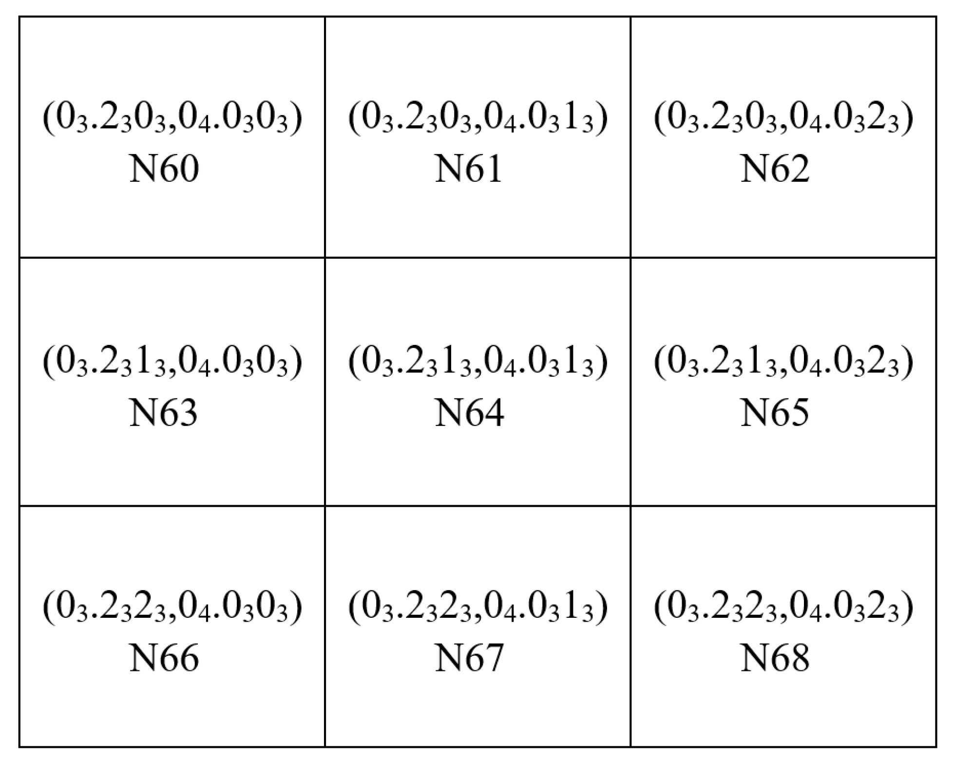
Finally, the rHEALPix DGGS has a cell indexing structure that allows us to efficiently determine cell adjacency directly from cell IDs [23]. By considering each numeric digit in the cell ID as a tuple whose two digits are the row and column numbers within the parent, we can determine the IDs of adjacent cells using math on the row and column numbers of the digit at the desired resolution. For example, if we wish to know the cells adjacent to cell , we first convert into notation (as described in Section 4 of [23]) which gives . Then, we add or subtract to the row and/or column number accordingly to determine the eight neighbouring cells in notation (Figure 2). Lastly, we simply convert notation back to cell ID.
3. Static Offset Regions
Consider a static IoT device (such as a smart water meter or smart parking meter) represented by a point location on the surface of the Earth and an offset region at a desired radius around this point defined using latitude-longitude coordinates in an ellipsoidal reference frame (such as WGS84). In order to model this point and offset region on the rHEALPix DGGS (or any DGGS), we need to quantize the point into a cell at a desired resolution and then efficiently determine which surrounding cells represent the offset region. Quantizing a point into a cell on the rHEALPix DGGS is a simple process using the inbuilt method (described in [22]) that calculates the unique ID of the desired resolution cell that contains the point. Efficiently determining the cells to represent the offset region is less trivial primarily because: (i) we need to limit the search space of cells so that every cell in the ellipsoidal grid at a desired resolution is not checked for inclusion and (ii) we must consider the curved surface of the ellipsoid and ensure that the set of ellipsoidal cells accurately represent the offset region [21].
Here we present methods that manipulate cell IDs and utilize the underlying indexing structure to: (i) limit the search space of cells that must be checked for inclusion in the offset region, (ii) determine cell containment in the offset region, (iii) perform efficient set operations on cell IDs, and (iv) limit costly geodetic computations. First, we consider the task of determining the set of cells that represent a static offset region using a single resolution approach (Section 3.1) and then we consider approaches that utilize the multiresolution hierarchy of the rHEALPix DGGS (Section 3.2).
3.1. Single Resolution
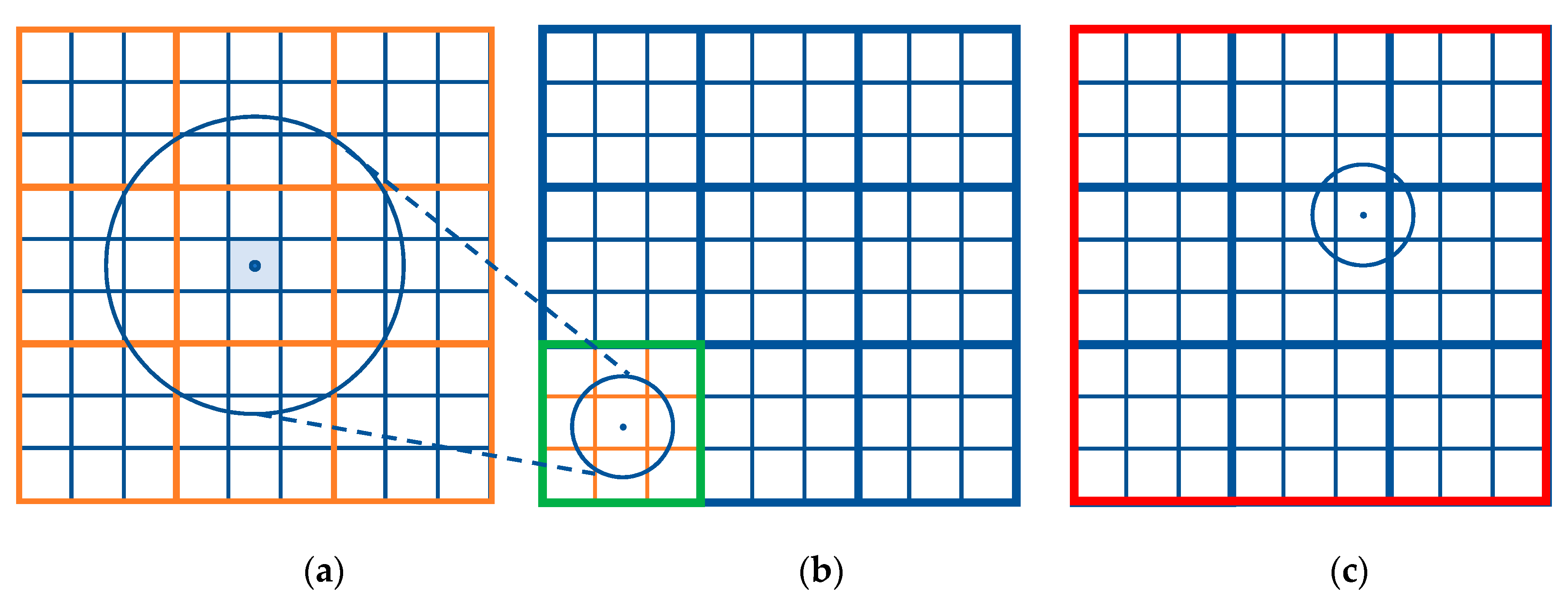
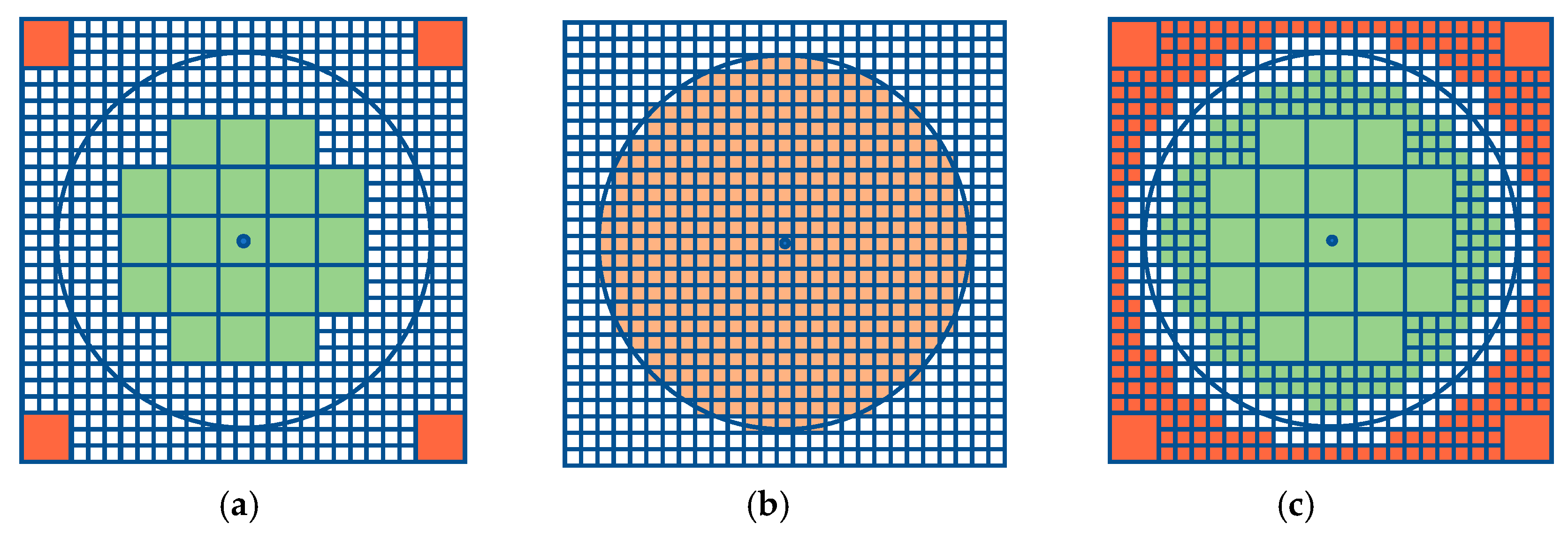
Consider a point that has been quantized into a cell at resolution and the circular offset region that we wish to model using a set of cells at resolution (Figure 3a). To limit the search space of cells, we could first determine the smallest bounding cell that contains (Figure 3b) by comparing the cell IDs of the latitude-longitude bounding box coordinates of from resolution to until they disagree (as described in Section 9 of [22]). Then, due to the congruent cell structure of the rHEALPix DGGS, we could simply use parent-child concatenation operations on cell IDs to determine the IDs of each cell at resolution within that must be checked for inclusion in . Although this process is straightforward, problems arise when is significantly larger than (Figure 3c) because it means checking a prohibitively large number of cells for inclusion. This is caused by spanning cells that have different parents at coarser resolutions (due to the fixed indexing structure that defines the hierarchical parent-child relationships) and is thus unavoidable.
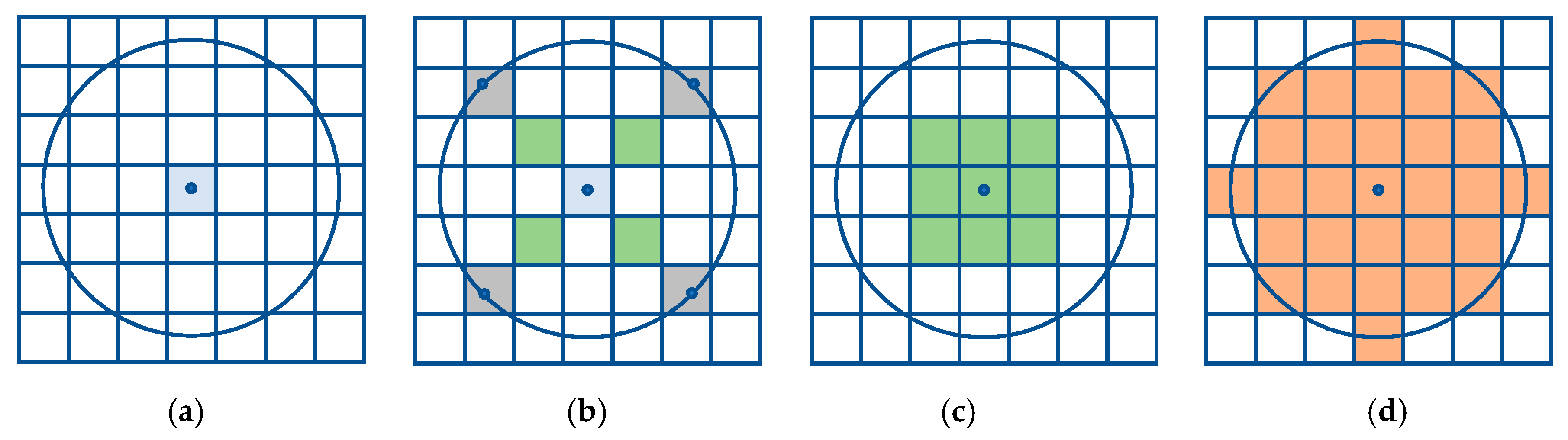
To reduce the search space to a more manageable and predictable size that is not affected by the cells spanned by , we propose using the latitude-longitude bounding box coordinates of to determine a rectangular bounding grid of cells at resolution that contain (Figure 4a). To do this, we take the four latitude-longitude coordinate pairs that represent the bounding box of , and convert them into their respective cell IDs at resolution . We then convert the cell IDs into notation and determine the minimum and maximum row and column values. Using these range of values, we can easily determine all cells that comprise in notation, which we lastly convert back to cell ID.
Although this approach limits the search space of cells that must be checked for inclusion in , we may still encounter the issue of checking a large number of cells, particularly if the cell size at resolution is small relative to the size of . To alleviate this issue, we wish to determine a rectangular inner grid of cells at resolution that are completely contained within (Figure 4c), so that we can automatically include these cells in without performing any further checks. To do this, we calculate the latitude-longitude coordinate pairs of four points on the boundary of using the coordinates of , the radius of , and the azimuths . These four azimuths are chosen in this study based on the fact that the largest planar rectangle circumscribed by a circle is a square (that said, these azimuths could be optimised to take into account the radius of and the curved surface of the Earth if desired). We then convert the four latitude-longitude coordinate pairs into their respective cell IDs at resolution . Importantly, because a point lies somewhere in its quantized cell, we observe that each of the four cells has a vertex neighbour closer to cell that must be fully contained in (Figure 4b). Knowing this, we can (i) convert each cell ID into notation and (ii) use math on the row and/or column value accordingly to determine the notation of the cell diagonally closer to . Then, we can determine minimum and maximum row and column values, and use these ranges to obtain all cells that comprise in notation, which we lastly convert back to cell ID.
Now that we know the cells comprising and , the only cells that must be checked for inclusion in , are those in the set . The last step is to decide on a criterion for determining whether a cell should be included in or not. For example, we could select all cells in the set that intersect the offset region , that are fully contained in , or whose nuclei are contained in . Although all three approaches converge to as resolution increases, we opt for the latter because a single geodetic distance computation (from to the cell nucleus) can classify a cell as being in or not, which helps to limit costly geodetic computations (Figure 4d shows the final set of cells that represent ). Note that we indicate using the geodetic coordinates of in the distance computation rather than the reference point of its quantized cell (i.e., the nucleus of ) because (i) retrieving the original vector data for a single point is feasible, unlike massive vector curves or polygons (as highlighted in [21]), and (ii) it accurately determines the cells in and avoids the discrepancies that would result from using the nucleus of , particularly at coarse resolutions. However, if we wish to avoid retrieving the geodetic coordinates of , then we can either (i) use the nucleus of if the quantization error at resolution is acceptable (e.g., at fine resolutions), or (ii) quantize into a cell at a finer resolution where and the quantization error at resolution is acceptable, and then use the nucleus of . The pseudocode to perform the single resolution method is provided in Algorithm 1.
| Algorithm 1. Pseudocode to perform the single resolution method |
| Input: point , offset radius , resolution |
Result: set of cells that represent the offset region
|
Although the proposed approach is demonstrated using the quadrilateral-based rHEALPix DGGS, it is not difficult to imagine how it could be adapted for triangular- and hexagonal-based DGGSs. For example, if we consider a hexagonal DGGS, rather than determine a rectangular bounding grid of cells , we could instead utilize the ring structure of neighbouring hexagons to determine the minimum bounding ring such that the resulting grid of cells contain . Similarly, rather than determine a rectangular inner grid of cells , we could determine the maximum inner ring such that all cells are fully contained within . An interesting benefit of this approach for hexagonal DGGSs, is that rings of neighbouring hexagons approximate a circle more closely than a rectangular grid of squares, therefore the set would have greater impact at limiting the number of cells that must be checked for inclusion in .
3.2. Multiresolution
Here we consider how the multiresolution hierarchy of the rHEALPix DGGS can be used to efficiently determine the set of cells at finer (or coarser) resolutions thereby removing the need to determine from scratch. First, we describe a method that utilizes the congruent cell structure (i.e., child cells are enclosed by the parent cell) and efficient cell adjacency operations on cell IDs to determine the cells in as resolution increases from a coarse resolution to a fine resolution , where . Second, we highlight a method that uses the alignment of cell nuclei to determine the cells in as resolution decreases from a fine resolution to a coarse resolution .
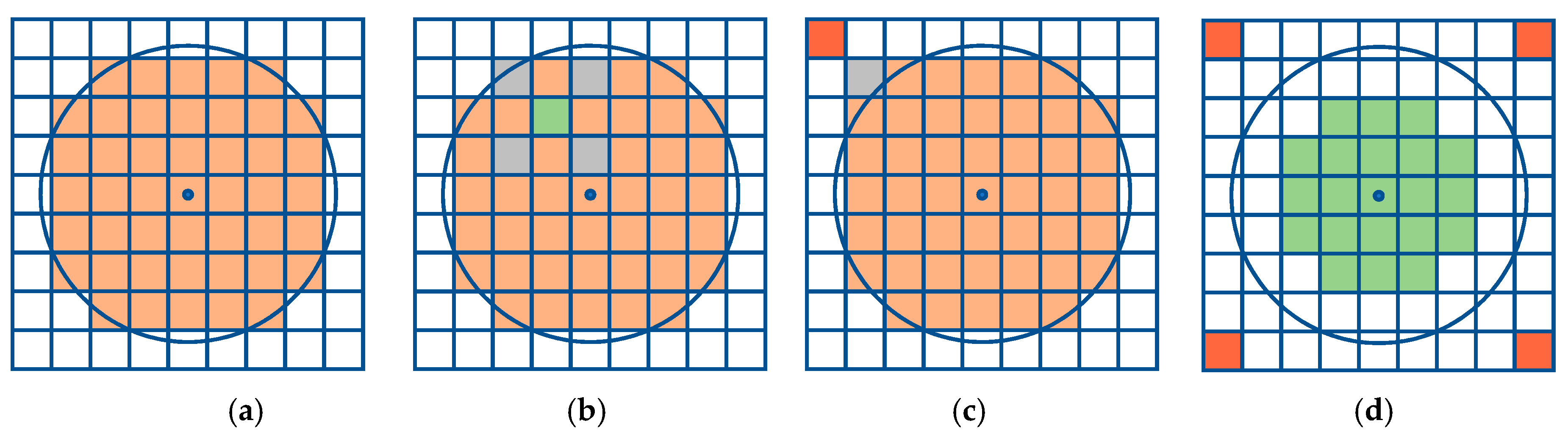
Consider an offset region , the rectangular bounding grid of cells that contain and the set of cells that represent at a coarse resolution (Figure 5a). Note that refers to the initial search space of cells at resolution . However, in the following method the search space at resolution is not equal to , so we will denote the search space of cells to avoid confusion. To determine the set of cells that represent , we first determine all cells in that are definitely fully contained in (Figure 5d) which allows us to automatically include their child cells in . To do this, we determine the four vertex neighbours of a given cell in (Figure 5b) using notation and math (as described in Section 2), and check that they are also in (using efficient set operations on cell IDs). We check the vertex neighbours because (i) if their nuclei are in then so are the cell vertices (since they constrain the vertices), (ii) it is more efficient than checking all eight neighbours (whose nuclei also constrain the vertices), and (iii) nuclei of edge neighbours may not necessarily constrain the vertices (particularly close to the boundary of ). Thus, if all vertex neighbours are in , we conclude that the given cell must be fully contained in .
Next, we determine all cells in that are definitely fully outside (Figure 5d) using a similar approach, except we check that the vertex neighbours are not in (Figure 5c). These cells, and all of their child cells, are marked as being outside of . The remaining cells are called “fringe cells” at resolution (Figure 5d), denoted , because they are located close to the boundary of and their corresponding child cells may or may not be in . The next step is to subdivide all cells in using simple parent-child concatenation operations on cell IDs, to determine the new search space of cells (Figure 6a). Lastly, we perform the single geodetic distance computation for all cells in to determine the cells that comprise (Figure 6b). If we wish to determine the set of cells that represent , we can iteratively repeat the process. For example, to determine the set of cells , we find all cells in that are definitely fully contained in and all cells in that are definitely fully outside (taking into account cells that were previously marked as fully inside or outside ). From here, we can determine the fringe cells (Figure 6c). We can then subdivide cells in to form , and subsequently test these cells for inclusion in . The pseudocode to perform the multiresolution method is provided in Algorithm 2.
| Algorithm 2. Pseudocode to perform the multiresolution method |
| Input: point , offset radius , coarse resolution , fine resolution , initial set of cells that represent the search space, initial set of cells that represent the offset region |
Result: set of cells that represent the offset region
|
Overall, by limiting the search space to child cells of the fringe cells, we can limit the number of costly geodetic distance computations and efficiently determine the cells in at finer resolutions. Furthermore, by using cell adjacency as the basis to determine cell containment in , we can utilize cell ID manipulation and perform efficient set operations on cell IDs. Lastly, by utilizing cell congruency and the underlying indexing structure, we can automatically include (or exclude) child cells in at finer resolutions using efficient parent-child concatenation operations on cell IDs. Note that with regards to the latter, if we only include the parent cell in at finer resolutions and not the respective child cells, we can model an offset region using a multiresolution set of cells . Importantly, will be geometrically equivalent to in terms of modelling , but will comprise fewer cells than (especially at increasingly fine resolutions) which would be beneficial (such as for memory storage or performance of inside/outside tests) if the number of cells in at a fine resolution becomes prohibitively large.
In terms of compatibility with other DGGSs, the proposed approach could be applied to triangular DGGSs because they also exhibit cell congruency. Hexagonal DGGSs (of which aperture 3, 4, and 7 are the most popular) have incongruent hierarchies however, which makes it more difficult to apply multiresolution approaches based on cell congruency. Interestingly though, the proposed approach of combining cell adjacency as the basis for cell containment in with cell nuclei as the basis for inclusion in , appears to be compatible with the aperture 7 hexagonal DGGS. In this type of hexagonal DGGS, the hexagonal shape of a parent cell is closely approximated by its seven child cells, despite not being fully contained. Notably, for a given cell at resolution , the seven respective child cells at resolution have centre points that are contained within . Thus, we observe that the centre points of the six adjacent cells of at resolution would not only constrain the vertices of , but also the vertices of all child cells of at any resolution greater than , as is the case for congruent cell shapes.
To end this section, we describe a method to efficiently determine the cells in as resolution decreases from a fine resolution to a coarse resolution using the aligned property of the rHEALPix DGGS. First, recall from Section 3.1 that a cell is included in if its nucleus is included in . Now consider the set of cells that represent at a fine resolution . In order to determine the cells in , we can utilize the fact that the nucleus of a parent cell at resolution is aligned with the nucleus of a child cell at resolution . On the rHEALPix DGGS with , the ID of an aligned child cell is always the same string as its parent cell ID except with the integer concatenated to the end (which can be seen in Figure 1). Consequently, to determine the cells in , we simply need to select all cell IDs in that end in 4, and then truncate each cell ID to remove the 4. This process can be iteratively repeated to determine the set of cells that represent . Note that by keeping track of the cell IDs that do not end in 4 at each resolution, we can move up and down the resolution levels by simply concatenating and appending or truncating and removing IDs from . Alternatively, in general, we note that if is the set of cells at a fine resolution , then we can determine the set of cells in at any resolution where by (i) selecting all cells in whose ID string ends in ’s and (ii) removing the ’s from each ID by truncating the string. Because this method is based on the alignment of cell nuclei, it could also be applied to triangular and hexagonal DGGSs that are aligned at cell centre points by manipulating cell IDs accordingly.
4. Mobile Offset Regions
In this section, we present methods to model an offset region around a mobile point (corresponding to the location of a mobile IoT device) that is quantized into a cell of a DGGS. This could be important for querying nearby cells (e.g., inside/outside tests), visualizing aggregate values in nearby cells, or representing a mobility neighbourhood to contextualise IoT data. For example, consider a mobile IoT device such as a smart phone or vehicle that generates a continuous stream of location-based point data (e.g., every 5 s). In this scenario, continually determining from scratch the set of cells at resolution that model the offset region around each incoming point may be impractical (e.g., if the incoming data rate is high or if represents a fine resolution). Therefore, we present methods that manipulate cell IDs directly to determine the cells in around each new point.
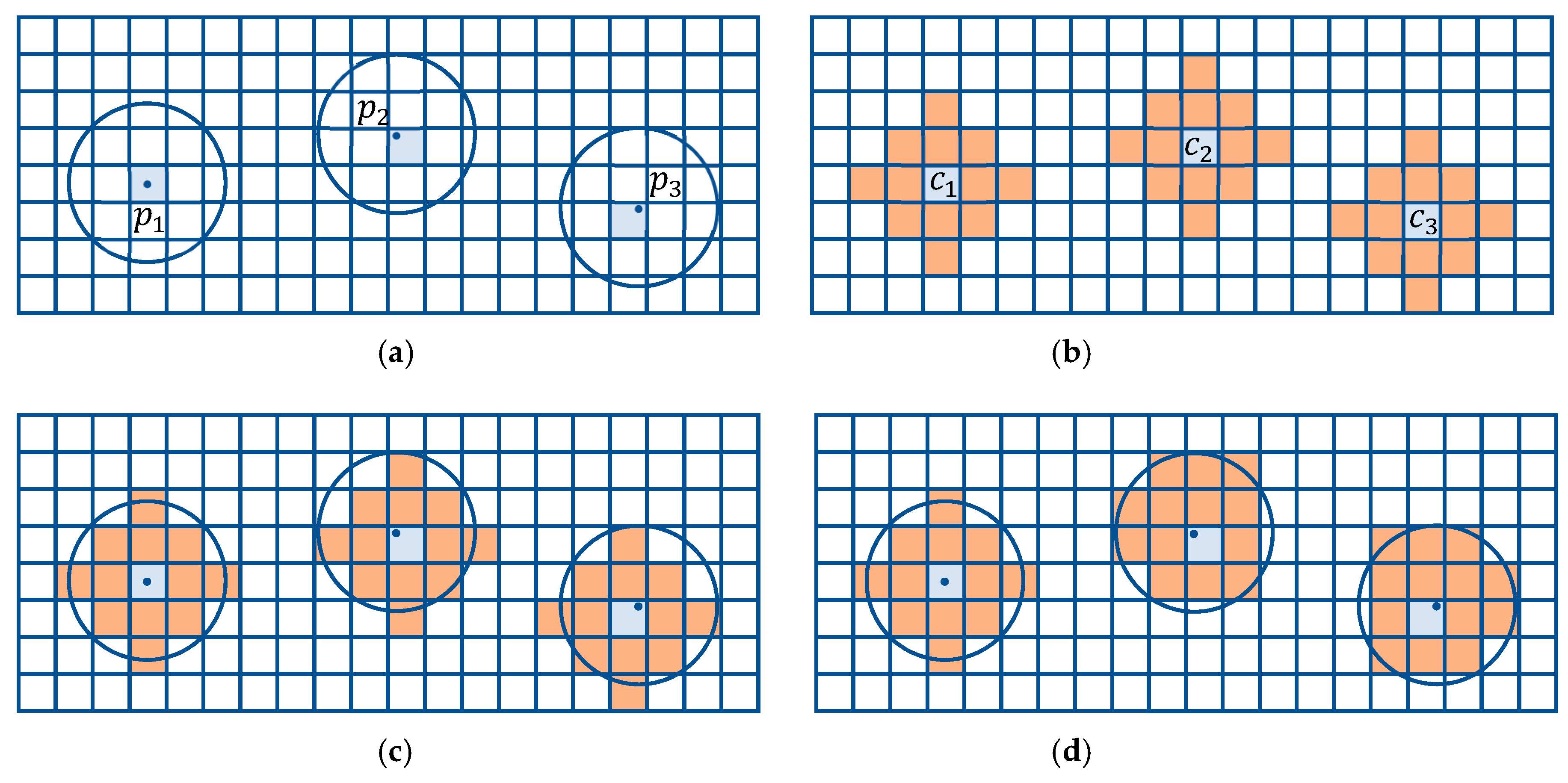
Consider the trajectory of a mobile IoT device represented by a time series of points and the corresponding series of offset regions at a desired radius around each defined using latitude-longitude coordinates in an ellipsoidal reference frame (e.g., WGS84). To model this scenario on the rHEALPix DGGS, we quantize each point into a cell at a desired resolution to determine the corresponding time series of cells , where is equal to (Figure 7a). The next step is to determine the series of sets of cells at resolution that model the offset regions . Rather than determine each from scratch, we can determine the cells in and then manipulate cell IDs directly to efficiently determine successive sets of cells.
First, let us consider modelling with cells at a fine resolution such that the quantization error is deemed acceptable for the IoT application (i.e., it is acceptable for to be centred on ). In this case, we determine the cells in using a static method from Section 3 whereby the nucleus (i.e., reference point) of is used in the geodetic distance computation, which ensures is centred on . Then, to determine the cells in , we first convert cells and to notation whereby the row and column values of and are denoted and respectively. Subsequently, we can compute the translation values from to using and . We can then apply to the row and column values of each cell in . Lastly, we can convert each cell in notation back to cell ID to determine the cells in . Note that because is centred on , will also be centred on (and so forth for all (Figure 7b). Furthermore, every cell at resolution has equal area so the total areal coverage of each remains constant. To determine the cells in , we can compute the translation values from to using and , which we can then apply to all cells in . Repeating this process for each consecutive pair of cells in allows us to efficiently model a mobile offset region at fine resolutions.
Now let us consider modelling with cells at a coarse resolution such that the quantization error at resolution is unacceptable (i.e., we want to be centred on ). In this case, we cannot simply determine cells in based on the change between and , because ignoring the actual change between and will result in discrepancies (Figure 7c). Consequently, we propose quantizing each into a cell at resolution where and the quantization error at resolution is deemed acceptable for the IoT application. We can then determine which is centred on . Subsequently, we can determine the translation values between and which can then be applied to all cells in to get . Lastly, we can use the alignment method described in Section 3.2 to determine the cells in at resolution . This approach ensures each is more accurately centred on , albeit with an accuracy relative to the quantization error at resolution (Figure 7d).
5. Results
In this section, we present a variety of results produced by applying the proposed methods to model static offset regions (Section 5.1) and mobile offset regions (Section 5.2).
5.1. Static Offset Regions
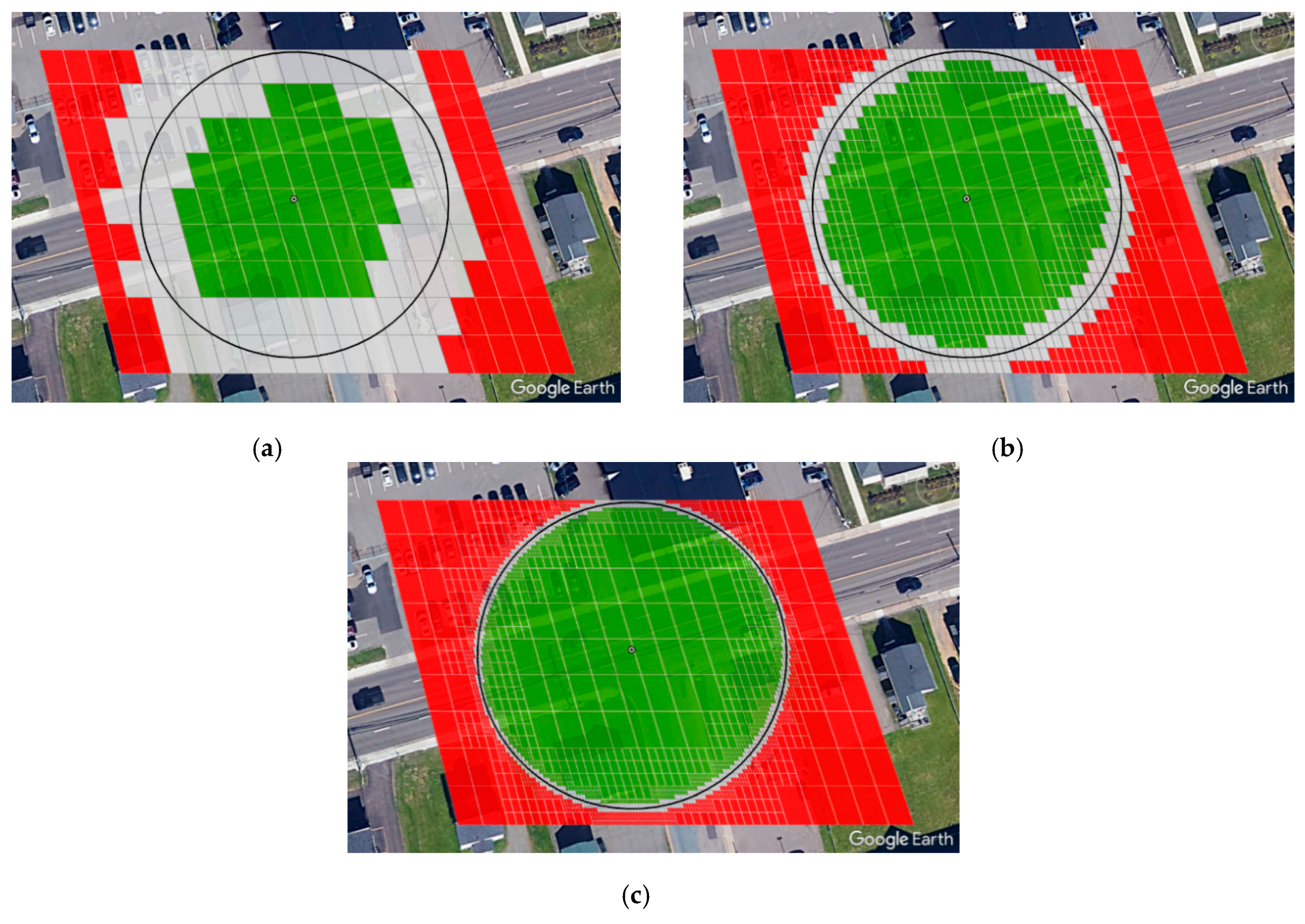
Figure 8 shows an offset region with 30 m radius around an arbitrary point in New Brunswick, Canada modelled at three successive resolutions (visualized in Google Earth). Figure 8a shows the offset region modelled at resolution 13 ( m ellipsoidal cell width) which represents a coarse resolution. Figure 8b,c show the offset region modelled at resolutions 14 ( m ellipsoidal cell width) and 15 ( m ellipsoidal cell width) respectively, which represent successively finer resolutions.
Recall that a key benefit of the multiresolution method is limiting the search space to child cells of the fringe cells at successive resolutions. To illustrate this, Figure 9 shows the fringe cells for the offset region from Figure 8 at resolutions 13, 14, and 15, along with the cells that are marked as fully inside or fully outside the offset region at successive resolutions (visualized in Google Earth).
To gain a better understanding of the improved efficiency that could be achieved by using the multiresolution method instead of the single resolution method, we compared the computation speeds of the two methods for determining the cells in the offset region from Figure 8 at resolutions 14, 15, and 16. For the multiresolution method, we used the resolution 13 set of cells as the initial coarse resolution. Tests were performed using the Python programming language on a 64-bit Windows 10 machine with an Intel Core i5-3570S CPU and 8 GB of RAM. Note that the open source GeoPy Python package (https://pypi.org/project/geopy/) was used to calculate the geodetic distance from point location to cell nucleus. Table 1 shows the average computation speeds for both methods.
Evidently, the multiresolution method significantly reduces computation speed as resolution increases. At resolution 14, there are approximately 31% less cells in the search space and as a result, fewer cells must undergo the costly geodetic distance check which leads to a reduction in computation speed of approximately 34%. At resolutions 15 and 16, the benefit of the multiresolution method becomes even clearer, as demonstrated by the significant reduction in computation speed (approximately 67% and 86% respectively). This is because the search space of cells is derived from the fringe cells which converges to the boundary of the offset region at finer resolutions (as shown in Figure 9), and is thus significantly smaller than the search space of cells in the single resolution method (e.g., 7020 cells versus 74886 cells at resolution 16). Moreover, the number of cells in the search space at successive resolutions increases by approximately a factor of three, compared to approximately a factor of nine for the single resolution method. Consequently, the cumulative number of cells that must be distance checked in the multiresolution method is far less than the single resolution method (e.g., 9963 cells versus 74886 cells at resolution 16).
5.2. Mobile Offset Regions
Recall that modelling a mobile offset region at a coarse resolution will result in discrepancies if cells in are determined based on the change between and . In order to gain a better understanding of these discrepancies and the improved accuracy that could be achieved using the proposed method of utilizing cells in with the alignment method to determine cells in , we computed the cells in a 30 m offset region around a series of 304 points using both methods at resolutions 12 ( m ellipsoidal cell width) and 13 ( m ellipsoidal cell width) and compared the results with the true set of cells determined using a static offset method from Section 3. Each point represents the location of a bus (considered as an IoT device) in a single trip of approximately 30 min. This data was extracted from real world Automatic Vehicle Location (AVL) feeds pulled every 5 s from buses of the Codiac transit network in Greater Moncton, New Brunswick, Canada. At each point , the error between the set of cells and true set of cells was calculated using Equation (1) which determines the number of cells that differ between the two sets. These values were averaged over the number of points to determine the mean cell error and standard deviation. Table 2 shows the error statistics when cells in are centred on and Table 3 shows the error statistics using the proposed method.
As shown in Table 2, there are clear discrepancies if cells in are centred on at coarse resolutions. For example, no at resolution 12 exactly matched the true set of cells (i.e., 100% of offsets were incorrect) and the average cell error for any was three cells. A similar pattern occurred at resolution 13, where 99.7% of offsets were incorrect and the average cell error was eight cells. However, these discrepancies can be reduced using the proposed method as shown in Table 3. At resolution 12, only 49.7% and 17.4% of offsets were incorrect and the average cell error for any was reduced to 0.7 cells and 0.2 cells when the value of was equal to 13 and 14 respectively. At resolution 13, 94.4% and 39.1% of offsets were incorrect and the average cell error for any was reduced to 3 cells and 0.6 cells when the value of was equal to 14 and 15 respectively.
Overall, it is evident that the average cell error for any decreases as increases. Moreover, at both resolution 12 and 13, average cell error is already less than 10% of the corresponding value in Table 2 when . This is because each cell is subdivided into nine child cells at successive resolutions which significantly reduces quantization error as increases (for apertures less than nine, we would expect average cell error to decrease more gradually). In addition, the number of occasions where exactly matched (i.e., cell error was equal to zero) increased as increased, as shown by the decrease in percentage of offsets that were incorrect. However, we note that the percentages are higher at resolution 13 most likely because there are more cells in (approximately 85 at resolution 13 versus 11 at resolution 12) which makes achieving an exact match with the cells in more difficult. On a further note, it is important to mention that increasing the value of significantly increases the number of cells in that must be manipulated in order to determine the cells in at a coarser resolution (as shown by the number of cells in the offset at resolution ). Therefore, to alleviate the associated computational cost of increasing , a valuable direction for future work would be to represent as a multiresolution set of cells (which contains significantly fewer cells) and explore methods of determining the cells in based on the translation values between and .
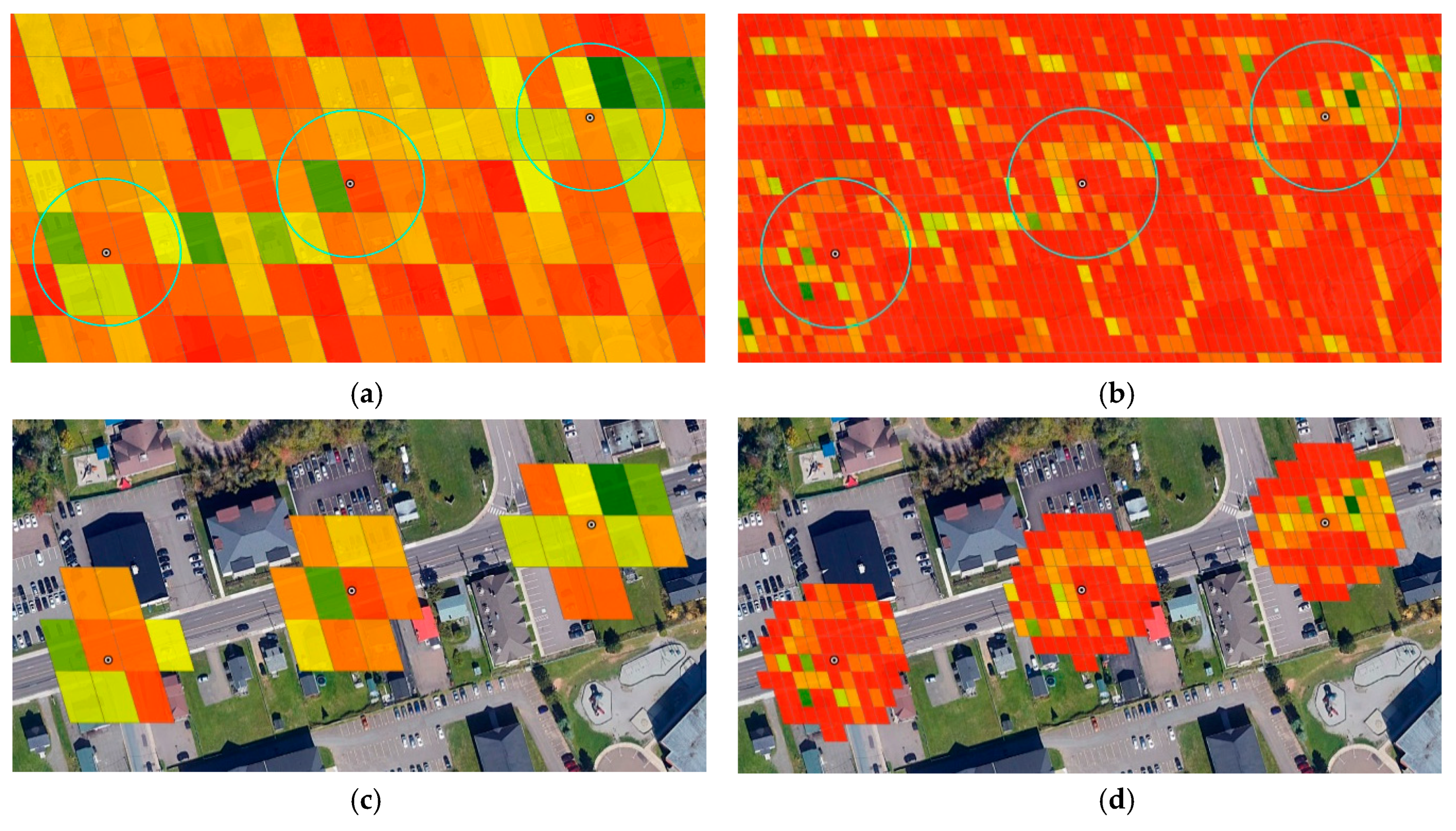
Lastly, Figure 10 illustrates how we can apply the proposed method to model mobile offset regions at coarse resolutions. Figure 10a,b show three successive point locations of a mobile IoT device (e.g., vehicle or smart phone) surrounded by a 30 m offset region and cells at resolution 12 ( m ellipsoidal cell width) and 13 ( m ellipsoidal cell width) respectively, that are coloured to simulate values derived from aggregating huge volumes of point data (e.g., noise level, air pollution, or ride-sharing data). By applying the proposed method with , we can determine and visualize the cells that surround each point as shown in Figure 10c,d (visualized in Google Earth).
6. Conclusions
With the huge volume of location-based point data being generated by IoT devices and subsequent rising interest from the Digital Earth community, a need has emerged for spatial operations that are compatible with Digital Earth and the underlying DGGS framework. To this end, we have presented methods of modelling an offset region around the point location of an IoT device (both static and mobile) that is quantized into a cell of a DGGS. Notably, these methods illustrate how the underlying indexing structure of a DGGS can be utilized to determine the cells in an offset region at different spatial resolutions. In particular, the proposed methods make use of cell congruency, alignment of cell nuclei, cell ID manipulation, and set operations on cell IDs to determine cell adjacency and topological relationships in support of modelling static and mobile offset regions. The proposed methods have been implemented to provide illustrative results, to show the computational speed gains of a multiresolution approach for modelling static offset regions at fine resolutions, and applied to show how cells of a mobile offset region can be determined and visualized at coarse resolutions.
With regards to modelling static offset regions, more research work is needed to develop efficient multiresolution approaches for hexagonal DGGSs that overcome the issue of an incongruent hierarchy. Along with pure-aperture hexagonal DGGSs, future work should also consider mixed-aperture hexagonal DGGSs [24] because they are a promising approach not constrained to have the same aperture at every resolution which provides greater control over cell area at each resolution and hence, greater flexibility in modelling offset regions.
In terms of modelling offset regions around mobile IoT device locations, our next step is to explore multiresolution approaches whereby a mobile offset region is represented as a multiresolution set of cells rather than a single resolution set of cells. In addition, we intend to explore the potential of using offset region cells to represent a mobility neighborhood around locations of a mobile IoT device in order to facilitate the important task of contextualizing IoT data. Because DGGS cells are ideally suited for integrating big geospatial data at different spatial resolutions, we anticipate that such an approach could prove to be beneficial.
Author Contributions
Conceptualization, David Bowater and Monica Wachowicz; Methodology, Software, Writing—Original Draft Preparation, David Bowater; Writing—Review & Editing, Supervision, Funding Acquisition, Monica Wachowicz. All authors have read and agreed to the published version of the manuscript.
Funding
This research was supported by the NSERC/Cisco Industrial Research Chair (Grant IRCPJ 488403-14).
Acknowledgments
The authors would like to thank the anonymous reviewers for their valuable comments.
Conflicts of Interest
The authors declare no conflict of interest.
References
- Van der Zee, E.; Scholten, H. Spatial dimensions of big data: Application of geographical concepts and spatial technology to the internet of things. In Big Data and Internet of Things: A Roadmap for Smart Environments; Bessis, N., Dobre, C., Eds.; Springer: Cham, Switzerland, 2014; pp. 137–168. [Google Scholar] [CrossRef]
- Cao, H.; Wachowicz, M. The design of an IoT-GIS platform for performing automated analytical tasks. Comput. Environ. Urban Syst. 2019, 74, 23–40. [Google Scholar] [CrossRef]
- Kamilaris, A.; Ostermann, F. Geospatial analysis and the internet of things. ISPRS Int. J. Geo Inf. 2018, 7, 269. [Google Scholar] [CrossRef] [Green Version]
- Sun, G.; Chang, V.; Ramachandran, M.; Sun, Z.; Li, G.; Yu, H.; Liao, D. Efficient location privacy algorithm for Internet of Things (IoT) services and applications. J. Netw. Comput. Appl. 2017, 89, 3–13. [Google Scholar] [CrossRef] [Green Version]
- Eldrandaly, K.A.; Abdel-Basset, M.; Shawky, L.A. Internet of spatial things: A new reference model with insight analysis. IEEE Access 2019, 7, 19653–19669. [Google Scholar] [CrossRef]
- Granell, C.; Kamilaris, A.; Kotsev, A.; Ostermann, F.O.; Trilles, S. Internet of things. In Manual of Digital Earth; Guo, H., Goodchild, M., Annoni, A., Eds.; Springer: Singapore, 2020; pp. 387–423. [Google Scholar] [CrossRef] [Green Version]
- Mahdavi-Amiri, A.; Alderson, T.; Samavati, F. A survey of digital earth. Comput. Graph. 2015, 53, 95–117. [Google Scholar] [CrossRef]
- Alderson, T.; Purss, M.; Du, X.; Mahdavi-Amiri, A.; Samavati, F. Digital earth platforms. In Manual of Digital Earth; Guo, H., Goodchild, M., Annoni, A., Eds.; Springer: Singapore, 2020; pp. 25–54. [Google Scholar] [CrossRef] [Green Version]
- Sahr, K.; White, D. Discrete global grid systems. In Proceedings of the 30th Symposium on the Interface, Computing Science and Statistics, Minneapolis, MN, USA, 13–16 May 1998; pp. 269–278. [Google Scholar]
- Sahr, K.; White, D.; Kimerling, A.J. Geodesic discrete global grid systems. Cartogr. Geogr. Inf. Sci. 2003, 30, 121–134. [Google Scholar] [CrossRef] [Green Version]
- Topic 21: Discrete Global Grid Systems Abstract Specification. Available online: http://docs.opengeospatial.org/as/15-104r5/15-104r5.html (accessed on 2 August 2018).
- Amiri, A.; Samavati, F.; Peterson, P. Categorization and conversions for indexing methods of discrete global grid systems. ISPRS Int. J. Geo Inf. 2015, 4, 320–336. [Google Scholar] [CrossRef]
- Li, Z. Geospatial Big Data Handling with High Performance Computing: Current Approaches and Future Directions. 2019. Available online: https://arxiv.org/abs/1907.12182 (accessed on 21 March 2020).
- Purss, M.B.J.; Peterson, P.R.; Strobl, P.; Dow, C.; Sabeur, Z.A.; Gibb, R.G.; Ben, J. Datacubes: A discrete global grid systems perspective. Cartogr. Int. J. Geogr. Inf. Geovis. 2019, 54, 63–71. [Google Scholar] [CrossRef]
- Sirdeshmukh, N.; Verbree, E.; Oosterom, P.V.; Psomadaki, S.; Kodde, M. Utilizing a discrete global grid system for handling point clouds with varying locations, times, and levels of detail. Cartogr. Int. J. Geogr. Inf. Geovis. 2019, 54, 4–15. [Google Scholar] [CrossRef] [Green Version]
- Yao, X.; Li, G.; Xia, J.; Ben, J.; Cao, Q.; Zhao, L.; Ma, Y.; Zhang, L.; Zhu, D. Enabling the big earth observation data via cloud computing and DGGS: Opportunities and challenges. Remote Sens. 2019, 12, 62. [Google Scholar] [CrossRef] [Green Version]
- Birk, F. Design and Implementation of a Scalable Crowdsensing Platform for Geospatial Data. Master’s Thesis, Ulm University, Ulm, Germany, 2018. [Google Scholar]
- H3: Uber’s Hexagonal Hierarchical Spatial Index. Available online: https://eng.uber.com/h3/ (accessed on 27 September 2019).
- Sahr, K. On the optimal representation of vector location using fixed-width multi-precision quantizers. Int. Arch. Photogramm. Remote Sens. Spat. Inf. Sci. ISPRS Arch. 2013, 40, 1–8. [Google Scholar] [CrossRef] [Green Version]
- Purss, M.B.J.; Liang, S.; Gibb, R.; Samavati, F.; Peterson, P.; Ben, J.; Dow, C.; Saeedi, S. Applying discrete global grid systems to sensor networks and the Internet of Things. In Proceedings of the IEEE International Geoscience and Remote Sensing Symposium (IGARSS), Fort Worth, TX, USA, 23–28 July 2017; pp. 5581–5583. [Google Scholar] [CrossRef]
- Alderson, T.; Mahdavi-Amiri, A.; Samavati, F. Offsetting spherical curves in vector and raster form. Vis. Comput. 2018, 34, 973–984. [Google Scholar] [CrossRef]
- Gibb, R.; Raichev, A.; Speth, M. The rHEALPix Discrete Global Grid System. 2016. Available online: https://datastore.landcareresearch.co.nz/dataset/rhealpix-discrete-global-grid-system (accessed on 17 July 2018). [CrossRef]
- Gibb, R.G. The rHEALPix Discrete Global Grid System. In IOP Conference Series: Earth and Environmental Science, Proceedings of the 9th Symposium of the International Society for Digital Earth (ISDE), Halifax, NS, Canada, 5–9 October 2015; IOP Publishing: Bristol, UK, 2016. [Google Scholar] [CrossRef] [Green Version]
- Sahr, K. Central place indexing: Hierarchical linear indexing systems for mixed-aperture hexagonal discrete global grid systems. Cartogr. Int. J. Geogr. Inf. Geovis. 2019, 54, 16–29. [Google Scholar] [CrossRef]
Figure 1.
Planar and ellipsoidal grids (based on the (0, 0)-rHEALPix projection) of the rHEALPix DGGS with at (a) resolution and (b) resolution . (Source: [23])
Figure 1.
Planar and ellipsoidal grids (based on the (0, 0)-rHEALPix projection) of the rHEALPix DGGS with at (a) resolution and (b) resolution . (Source: [23])

Figure 2.
Adjacent cells of cell N64 expressed using notation and cell IDs.

Figure 3.
(a) A point, its quantized cell at resolution (shown in light blue), and an offset region. (b) The bounding cell of the offset region from (a) at resolution (shown in green). (c) The bounding cell of an offset region at a different location at resolution (shown in red).
Figure 3.
(a) A point, its quantized cell at resolution (shown in light blue), and an offset region. (b) The bounding cell of the offset region from (a) at resolution (shown in green). (c) The bounding cell of an offset region at a different location at resolution (shown in red).

Figure 4.
(a) A point, its quantized cell (shown in light blue), and a rectangular grid of cells that bound the offset region. (b) Each of the four grey cells has a vertex neighbor (shown in green) closer to the light blue cell that is fully contained in the offset region. (c) A rectangular grid of cells that are fully contained in the offset region (shown in green). (d) The cells that represent the offset region (shown in orange).

Figure 5.
(a) The set of cells that represent the offset region at resolution (shown in orange). (b) A cell in is marked as fully inside the offset region (shown in green) if its vertex neighbours (shown in grey) are also in . (c) A cell not in is marked as fully outside the offset region (shown in red) if its vertex neighbours (shown in grey) are also not in . (d) Cells at resolution i marked as fully outside and fully inside the offset region (shown in red and green respectively). White cells represent the fringe cells at resolution i.

Figure 6.
(a) White cells represent the search space at resolution . (b) Orange cells represent the offset region at resolution . (c) Red cells at resolution and are fully outside the offset region while green cells are fully inside (based on vertex neighbour check). White cells represent the fringe cells at resolution .

Figure 7.
(a) A series of points (quantized cells are shown in light blue) representing locations of a mobile IoT device and corresponding offset regions. (b) Offset cells centred on and subsequently determined offset cells centred on and . (c) Offset cells centred on and may have discrepancies. (d) Offset cells centred on each point.

Figure 8.
An offset region with 30 m radius modelled at resolution (a) 13, (b) 14, and (c) 15 (©2020 Google Earth).
Figure 8.
An offset region with 30 m radius modelled at resolution (a) 13, (b) 14, and (c) 15 (©2020 Google Earth).

Figure 9.
An offset region with 30 m radius and fringe cells of the multiresolution method at resolution (a) 13, (b) 14, and (c) 15 (shown in light grey). Cells marked as fully outside the offset region are shown in red and cells marked as fully inside the offset region are shown in green (©2020 Google Earth).

Figure 10.
(a,b) A series of points representing locations of a mobile IoT device surrounded by a 30 m offset region and cells colored to simulate aggregate values at resolution 12 and 13 respectively. (c,d) Visualizing offset region cells from (a,b) respectively around each point (©2020 Google Earth).


Table 1.
Computation speeds for determining cells in the 30 m offset region from Figure 8 at different resolutions.
Table 1.
Computation speeds for determining cells in the 30 m offset region from Figure 8 at different resolutions.
| Cell Resolution | Cells in Offset | Single Resolution Method | Multiresolution Method | Time Reduction (%) | ||
|---|---|---|---|---|---|---|
| Cells in Search Space | Time (s) | Cells in Search Space | Time (s) | |||
| 13 | 83 | 132 | 0.05 | - | - | - |
| 14 | 762 | 976 | 0.38 | 675 | 0.25 | 34 |
| 15 | 6837 | 8574 | 3.3 | 2268 | 1.1 | 67 |
| 16 | 61,633 | 74,886 | 29 | 7020 | 4.2 | 86 |
Table 2.
Error statistics for modelling a mobile 30 m offset region at coarse resolutions when cells in are centred on .
Table 2.
Error statistics for modelling a mobile 30 m offset region at coarse resolutions when cells in are centred on .
| Cell Resolution | Cells in Offset | Cell Error | Offsets Incorrect (%) | |
|---|---|---|---|---|
| Mean | Std. Dev. | |||
| 12 | 11 | 3 | 1 | 100 |
| 13 | 85 | 8 | 3 | 99.7 |
Table 3.
Error statistics for modelling a mobile 30 m offset region at coarse resolutions using the proposed method.
Table 3.
Error statistics for modelling a mobile 30 m offset region at coarse resolutions using the proposed method.
| Cell Resolution | Resolution | Resolution | ||||||
|---|---|---|---|---|---|---|---|---|
| Cell Error | Offsets Incorrect (%) | Cells in Offset at res. | Cell Error | Offsets Incorrect (%) | Cells in Offset at res. | |||
| Mean | Std. Dev. | Mean | Std. Dev. | |||||
| 12 | 0.7 | 0.8 | 49.7 | 85 | 0.2 | 0.5 | 17.4 | 759 |
| 13 | 3 | 2 | 94.4 | 759 | 0.6 | 0.9 | 39.1 | 6855 |
© 2020 by the authors. Licensee MDPI, Basel, Switzerland. This article is an open access article distributed under the terms and conditions of the Creative Commons Attribution (CC BY) license (http://creativecommons.org/licenses/by/4.0/).
Share and Cite
MDPI and ACS Style
Bowater, D.; Wachowicz, M. Modelling Offset Regions around Static and Mobile Locations on a Discrete Global Grid System: An IoT Case Study. ISPRS Int. J. Geo-Inf. 2020, 9, 335. https://doi.org/10.3390/ijgi9050335
AMA Style
Bowater D, Wachowicz M. Modelling Offset Regions around Static and Mobile Locations on a Discrete Global Grid System: An IoT Case Study. ISPRS International Journal of Geo-Information. 2020; 9(5):335. https://doi.org/10.3390/ijgi9050335
Chicago/Turabian StyleBowater, David, and Monica Wachowicz. 2020. "Modelling Offset Regions around Static and Mobile Locations on a Discrete Global Grid System: An IoT Case Study" ISPRS International Journal of Geo-Information 9, no. 5: 335. https://doi.org/10.3390/ijgi9050335
Note that from the first issue of 2016, this journal uses article numbers instead of page numbers. See further details here.