Correlance and discordance: computable measures of nonlocal correlation

Abstract

We present six new measures of nonlocal correlation for discrete multipartite quantum systems; correlance, statance, probablance, strong discordance, discordance, and diagonal discordance. The correlance measures all nonlocal correlations (even bound entanglement) and is exactly computable for all pure and mixed states. Statance and probablance are not yet computable, but motivate the strong discordance (for nonlocal correlation beyond that achievable by a strictly classical state), discordance (a measure of all nonlocal correlation in distinguishably quantum states), and diagonal discordance (for nonlocal correlation in diagonal states), all of which are exactly computable for all states. We discuss types of correlation and notions of classicality and compare correlance, strong discordance, and discordance to quantum discord. We also define diagonal correlance to handle strictly classical probability distributions, providing a powerful tool with wide-ranging applications.

Appendices

A: Brief review of reduced states

Let the multimode reduction from N-mode parent state$\rho$ to a composite subsystem of $S\in 1,\ldots ,N$ possibly noncontiguous and reordered modes $\mathbf {m} \equiv (m_1 , \ldots ,m_S)$ be

$$\begin{aligned} {\check{\rho }^{(\mathbf {m})}} \equiv \text {tr}_{\mathbf {\overline{m}}} (\rho ), \end{aligned}$$

(67)

where the symbol in ${\check{\rho }^{(\mathbf {m})}}$ indicates that it is a reduction of $\rho$ (and not merely an isolated system of the same size as mode group $\mathbf {m}$), and the bar in $\mathbf {\overline{m}}$ means “not $\mathbf {m}$,” meaning that we trace over all modes whose labels are not in $\mathbf {m}$. See Appendix B of [18] for details.

B: Quantum discord definition

A suggested definition for quantum discord [11, 13] is

$$\begin{aligned} \mathcal {Q}(\rho )\equiv \mathcal {I}(\rho )-\mathcal {C}(\rho ), \end{aligned}$$

(68)

with $\mathcal {I}(\rho )$ from (1), where the classical correlation is

$$\begin{aligned} \mathcal {C}(\rho )\equiv \mathop {\max }\limits _{\{ P_k^{(2)} \} } \left[ {\mathcal {I}(\rho |\{ P_k^{(2)} \} )} \right] , \end{aligned}$$

(69)

where we define

$$\begin{aligned} \mathcal {I}(\rho |\{ P_k^{(2)} \} )\equiv S({\check{\rho }^{(1)}}) - S(\rho |\{ P_k^{(2)} \} ) \end{aligned}$$

(70)

as the quantum mutual information of the von Neumann measurement with projection operators $\{ P_k^{(2)} \}$ for mode 2, where

$$\begin{aligned} S(\rho |\{ P_k^{(2)} \} ) \equiv \sum \nolimits _k {p_k } S(\rho _k ) \end{aligned}$$

(71)

is the conditional von Neumann entropy given this measurement, where $p_k \equiv \text {tr}[(I^{(1)} \otimes P_k^{(2)} )\rho (I^{(1)} \otimes P_k^{(2)} )^ \dag ]$ are the probabilities of conditional measurement-outcome states $\rho _k \equiv \frac{1}{{p_k }}(I^{(1)} \otimes P_k^{(2)} )\rho (I^{(1)} \otimes P_k^{(2)} )^ \dag$.

C: Purity

Recall that the purity of $\rho$ is the trace of its square,

$$\begin{aligned} P \equiv P(\rho ) \equiv \text {tr}(\rho ^2 ), \end{aligned}$$

(72)

with range $P \in [\frac{1}{n},1]$ for an isolated system, and $\rho$ is pure iff $P=1$. Otherwise, if $P<1$ then $\rho$ is mixed. Thus, for mode m, $P(\rho ^{(m)} ) \in [\frac{1}{{n_m }},1]$ for an isolated mode m.

Beware: if the parent state $\rho$ is not a product state, then its reductions ${\check{\rho }^{(m)}}$ can have constraints on the limits of their purity, as proved in [18]. The reason (3) has no nonlocal correlation is that its tensor product ensures that each reduction (marginal state) is ${\check{\rho }^{(m)}}=\rho ^{(m)}$, and therefore has no dependence on any other modes.

D: Some basic details about entanglement

In separable states, as in (4), notice that the probabilities $p_j$ do not need any special structure for (4) to be satisfied, and that the decomposition states $\rho _j$ merely need product form, but not mode independence. Therefore, product form of the full state is not necessary for separability in general. However, for pure states, product form is both necessary and sufficient for separability.

For example, in a two-qubit system where each qubit has a generic basis with labels starting on 1 (our convention in this paper) as $\{ |1\rangle ,|2\rangle \}$, the pure state $|\psi \rangle = ac|1\rangle \otimes |1\rangle + ad|1\rangle \otimes |2\rangle + bc|2\rangle \otimes |1\rangle + bd|2\rangle \otimes |2\rangle$ is separable because it can be factored as $|\psi \rangle = (a|1\rangle + b|2\rangle ) \otimes (c|1\rangle + d|2\rangle )$, so that $\rho = |\psi \rangle \langle \psi | = \rho ^{(1)} \otimes \rho ^{(2)}$ where $\rho ^{(m)} = |\psi ^{(m)} \rangle \langle \psi ^{(m)} |$, and $|\psi ^{(1)} \rangle = a|1\rangle + b|2\rangle$ and $|\psi ^{(2)} \rangle = c|1\rangle + d|2\rangle$. In contrast, the pure state $|\varPhi ^ + \rangle = \frac{1}{{\sqrt{2} }}(|1\rangle \otimes |1\rangle + |2\rangle \otimes |2\rangle )$ is not separable so it is entangled (and happens to be maximally entangled) because it cannot be factored into a product form (since this example is for pure states).

E: Example of product form

To get product form for a two-qubit state $\rho = \sum \nolimits _j {p_j \rho _j }$ (and to demonstrate mode independence), Theorem 1 requires (5–8) by setting $\rho _j \equiv \rho _j^{(1)} \otimes \rho _j^{(2)}$ and

$$\begin{aligned} \begin{array}{*{20}l} {p_1 } &{} { = p_{(1,1)} } &{} { \equiv p_1^{(1)} p_1^{(2)} ,\;\;} &{} {\rho _1^{(1)} } &{} { = \rho _{(1,1)}^{(1)} } &{} { \equiv \rho _{(1)}^{(1)} ,\;\;} &{} {\rho _1^{(2)} } &{} { = \rho _{(1,1)}^{(2)} } &{} { \equiv \rho _{(1)}^{(2)} ,} \\ {p_2 } &{} { = p_{(1,2)} } &{} { \equiv p_1^{(1)} p_2^{(2)} ,\;\;} &{} {\rho _2^{(1)} } &{} { = \rho _{(1,2)}^{(1)} } &{} { \equiv \rho _{(1)}^{(1)} ,\;\;} &{} {\rho _2^{(2)} } &{} { = \rho _{(1,2)}^{(2)} } &{} { \equiv \rho _{(2)}^{(2)} ,} \\ {p_3 } &{} { = p_{(2,1)} } &{} { \equiv p_2^{(1)} p_1^{(2)} ,\;\;} &{} {\rho _3^{(1)} } &{} { = \rho _{(2,1)}^{(1)} } &{} { \equiv \rho _{(2)}^{(1)} ,\;\;} &{} {\rho _3^{(2)} } &{} { = \rho _{(2,1)}^{(2)} } &{} { \equiv \rho _{(1)}^{(2)} ,} \\ {p_4 } &{} { = p_{(2,2)} } &{} { \equiv p_2^{(1)} p_2^{(2)} ,\;\;} &{} {\rho _4^{(1)} } &{} { = \rho _{(2,2)}^{(1)} } &{} { \equiv \rho _{(2)}^{(1)} ,\;\;} &{} {\rho _4^{(2)} } &{} { = \rho _{(2,2)}^{(2)} } &{} { \equiv \rho _{(2)}^{(2)} ,} \\ \end{array} \end{aligned}$$

(73)

where all states in (73) are pure. Then $\rho$ becomes

(74)

with $\rho ^{(1)} \equiv p_1^{(1)} \rho _{(1)}^{(1)} + p_2^{(1)} \rho _{(2)}^{(1)}$ and $\rho ^{(2)} \equiv p_1^{(2)} \rho _{(1)}^{(2)} + p_2^{(2)} \rho _{(2)}^{(2)}$. Notice the redundant probabilities and decomposition states in (73); this is a consequence of applying Theorem 1. Also, if either or both mode reductions have lower rank, some of the probabilities in (73) will be zero.

Thus, the smallest maximum number of decomposition states required for any mixed product state is

$$\begin{aligned} r_{1}\cdots r_{N}=r, \end{aligned}$$

(75)

(which is also their minimum number of decomposition states) where the ranks of each single-mode reduction of the product state are $r_{m}\in 1,\ldots ,n_{m}$, and $r\equiv \text {rank}(\rho )$, which is just an application the well-known property for tensor products that $\text {rank}(A\otimes B)=\text {rank}(A)\text {rank}(B)$. In fact, by making mode-independent (MI) tensor products of the eigenstates of the reductions, and forming the corresponding probabilities from MI products of the eigenvalues of the reductions, we can always construct an r-member MI decomposition of any product state.

F: Proof of Theorem 1

Starting with a general mixed state,

$$\begin{aligned} \rho = \sum \nolimits _j {p_j \rho _j }, \end{aligned}$$

(76)

applying (5) gives a separable state,

$$\begin{aligned} \rho = \sum \nolimits _j {p_j \rho _j^{(1)} \otimes \cdots } \otimes \rho _j^{(N)}, \end{aligned}$$

(77)

which is not enough to definitely get product form. If we then also use (7), we get

$$\begin{aligned} \begin{array}{*{20}l} {\rho } &{} {=\sum \nolimits _j {(p_j^{(1)} \cdots p_j^{(N)} )\rho _j^{(1)} \otimes \cdots \otimes \rho _j^{(N)} }} \\ {} &{} {= \sum \nolimits _j {p_j^{(1)} \rho _j^{(1)} \otimes \cdots \otimes p_j^{(N)} \rho _j^{(N)} },} \\ \end{array} \end{aligned}$$

(78)

which is still not enough for product form because the indices are “locked” across the modes, indicating nonlocal correlation. Therefore, vectorizing the indices as

$$\begin{aligned} \rho = \sum \limits _{j_1 , \ldots ,j_N } {} p_{(j_1 , \ldots ,j_N )}^{(1)} \rho _{(j_1 , \ldots ,j_N )}^{(1)} \otimes \cdots \otimes p_{(j_1 , \ldots ,j_N ) }^{(N)} \rho _{(j_1 , \ldots ,j_N )}^{(N)}, \end{aligned}$$

(79)

and then applying both (8) and (6), we get

$$\begin{aligned} \begin{array}{*{20}l} {\rho } &{} {= \sum \nolimits _{j_1 } { \cdots \sum \nolimits _{j_N } {p_{j_1 }^{(1)} \rho _{j_1 }^{(1)} \otimes \cdots \otimes p_{j_N }^{(N)} \rho _{j_N }^{(N)} } }} \\ {} &{} {= (\sum \nolimits _{j_1 } {p_{j_1 }^{(1)} \rho _{j_1 }^{(1)} } ) \otimes \cdots \otimes (\sum \nolimits _{j_N } {p_{j_N }^{(N)} \rho _{j_N }^{(N)} } )} \\ {} &{} {= \rho ^{(1)} \otimes \cdots \otimes \rho ^{(N)}} \\ \end{array} \end{aligned}$$

(80)

where $\rho ^{(m)} \equiv \sum \nolimits _{j_m } {p_{j_m }^{(m)} \rho _{j_m }^{(m)} }$, which proves the sufficiency of (5–8) for product form, and thus the absence of all nonlocal correlation.

To prove the necessity of (5–8) for product form, we simply start from the product-form definition in (3),

$$\begin{aligned} \rho = \rho ^{(1)} \otimes \cdots \otimes \rho ^{(N)} . \end{aligned}$$

(81)

Then, since each mode’s state can be generally mixed as

$$\begin{aligned} \rho ^{(m)} = \sum \nolimits _{j_m } {p_{j_m }^{(m)} \rho _{j_m }^{(m)} } , \end{aligned}$$

(82)

we can put (82) into (81) to get

$$\begin{aligned} \rho = (\sum \nolimits _{j_1 } {p_{j_1 }^{(1)} \rho _{j_1 }^{(1)} } ) \otimes \cdots \otimes (\sum \nolimits _{j_N } {p_{j_N }^{(N)} \rho _{j_N }^{(N)} } ). \end{aligned}$$

(83)

Rearranging shows that product states must have form

$$\begin{aligned} \begin{array}{*{20}l} {\rho } &{} {= \sum \nolimits _{j_1 } { \cdots \sum \nolimits _{j_N } {p_{j_1 }^{(1)} \rho _{j_1 }^{(1)} \otimes \cdots \otimes p_{j_N }^{(N)} \rho _{j_N }^{(N)} } }} \\ {} &{} {= \sum \limits _{j_1 , \ldots ,j_N } {(p_{j_1 }^{(1)} \cdots p_{j_N }^{(N)} )\rho _{j_1 }^{(1)} \otimes \cdots \otimes \rho _{j_N }^{(N)} }.} \\ \end{array} \end{aligned}$$

(84)

Thus, line 2 of (84) verifies that this form is equivalent to product-form. Then, to show how (84) relates to the notation of a general mixed state, we can unify these all with a vector index only if each mode has redundantly defined quantities of the forms $p_{j_m }^{(m)} = p_{(j_1 , \ldots ,j_N )}^{(m)}$ and $\rho _{j_m }^{(m)} = \rho _{(j_1 , \ldots ,j_N )}^{(m)}$, regardless of the values of the indices of labels other than m, so then (84) becomes

(85)

and then if we abbreviate $p_j=p_j^{(1)} \cdots p_j^{(N)}$ and $\rho _j =$$\rho _j^{(1)} \otimes \cdots \otimes \rho _j^{(N)}$, then (85) takes the general form

$$\begin{aligned} \rho = \sum \nolimits _j {p_j \rho _j } , \end{aligned}$$

(86)

which shows that since we started from product states in (81) and used (5–8) to recover the form of a general state in (86), then (5–8) are necessary for product form. Thus, we have now proven that (5–8) are necessary and sufficient conditions for a state to have product form. $\square$

G: Proofs and caveats for the six families of nonlocal correlation

Here we develop some important facts about the six families of nonlocal correlation from Table 1.

1.1 G.1: Proof that all decomposition probabilities are expressible in product form without mode normalization

Given a set of normalized decomposition probabilities $\{ p_j \}$, we can always express them in product form as

$$\begin{aligned} p_j = \prod \nolimits _{m = 1}^N {p_j ^{(m)} } = p_j ^{(1)} \cdots p_j ^{(N)}\;\; \forall j, \end{aligned}$$

(87)

by using the parameterization

$$\begin{aligned} p_j ^{(m)} = p_j ^{x_m^2 (\varvec{\theta } ^{\{j\}} )}\;\; \forall j;\;\;m \in 1, \ldots ,N, \end{aligned}$$

(88)

where for each j, the $x_m (\varvec{\theta } ^{\{j\}} )$ for $m \in 1, \ldots ,N$ are N-dimensional unit-hyperspherical coordinates [31] with $N-1$ angles $\varvec{\theta } ^{\{j\}}\equiv (\theta _1^{\{j\}} , \ldots ,\theta _{N - 1}^{\{j\}} )$ which can be restricted to $\theta _k^{\{j\}} \in [0,\frac{\pi }{2}]$ for this application, with a different set for each j. These coordinates have the property that $\sum \nolimits _{m = 1}^N {x_m^2 (\varvec{\theta } ^{\{j\}} )} = 1\;\;\forall j$. Notice that in (88), we are setting each mode-specific factor $p_j ^{(m)}$ equal to the full probability $p_j$ raised to the power $x_m^2 (\varvec{\theta } ^{\{j\}} )$. Thus,

$$\begin{aligned} \begin{array}{*{20}l} {p_j } &{} {= p_j ^1 = p_j ^{x_1^2 (\varvec{\theta } ^{\{j\}} ) + \cdots + x_N^2 (\varvec{\theta } ^{\{j\}} )} = p_j ^{x_1^2 (\varvec{\theta } ^{\{j\}} )} \cdots p_j ^{x_N^2 (\varvec{\theta } ^{\{j\}} )}} \\ {} &{} {= p_j ^{(1)} \cdots p_j ^{(N)}\;\;\forall j,} \\ \end{array} \end{aligned}$$

(89)

which also works right to left, given (88). Therefore, we have proven that all decomposition probabilities are always expressible in product form as in (87), where we do not require mode normalization over j as $\sum \nolimits _j {p_j ^{(m)} } = 1\;\forall m$, which is actually impossible as we prove in Appendix G.2. $\square$

The consequence of (89) is that we do not need to define separate sets of families based on whether they have decompositions with product-form probabilities as $p_j = p_j ^{(1)} \cdots p_j ^{(N)}$, since such families would be redundant to other families with general probabilities $p_j$ and the same decomposition-state forms. For example, defining a family as $\rho = \sum \nolimits _j (p_j ^{(1)} \cdots p_j ^{(N)})\rho _j$ would be exactly the same as Family 1, which is $\rho = \sum \nolimits _j p_{j}\rho _j$ of Table 1.

1.2 G.2: Proof that product-form probabilities with mode normalization on the full decomposition index are impossible except trivially

Suppose we require that in addition to having product form (PF), the decomposition probabilities $p_j$ must also have mode normalization over the full decomposition index j, so that

$$\begin{aligned} p_j = \prod \nolimits _{m = 1}^N {p_j ^{(m)} } = p_j ^{(1)} \cdots p_j ^{(N)} \;\;\forall j;\;\;\sum \nolimits _j {p_j ^{(m)} } = 1\;\;\forall m, \end{aligned}$$

(90)

which is not the same thing as mode independence (MI) from (8) due to the sum over the full j rather than mode-specific index $j_m$ where $j \equiv (j_1 , \ldots ,j_N )$.

First, for the PF part, we can use the parameterization of Appendix G.1, which, together with the mode normalization over j, requires that

$$\begin{aligned} \sum \nolimits _j {p_j ^{(m)} } = \sum \nolimits _j {p_j ^{x_m^2 (\varvec{\theta } ^{\{ j\} } )} } = 1\;\;\forall m. \end{aligned}$$

(91)

For decompositions with D states, this requires that

$$\begin{aligned} p_1 ^{x_m^2 (\varvec{\theta } ^{\{ 1\} } )} + \cdots + p_D ^{x_m^2 (\varvec{\theta } ^{\{ D\} } )} = 1\;\;\forall m. \end{aligned}$$

(92)

Now, given that any collection of D real numbers on (0, 1] such as $\{p_{j}\}$ can be viewed as eigenvalues of some physical D-level state, then they are always exactly determined by a set of D equations for their power sums as

$$\begin{aligned} p_1^k + \cdots + p_D^k = \sum \nolimits _{j=1}^{D} {p_j^k } \equiv P_k , \end{aligned}$$

(93)

for integers $k \in 1, \ldots ,D$. Thus, (92) constitutes a set of generally additional constraints beyond the main set in (93), so together (92) and (93) form a generally overdetermined set of nonlinear equations.

It turns out that this overdetermined set does have solutions, but only for cases that are irrelevant for the purpose of defining nontrivial families of decompositions for probability correlation, as we now briefly explain.

One way to get a solution to an overdetermined set is to find conditions for which the additional constraints simplify to the main constraints (93). Since the powers of $p_j$ in (92) are squared unit-hyperspherical coordinates and therefore are each no greater than 1, then for a given m in (92), we can never achieve the condition of having both all powers being equal and all being integers, without preventing that for all other m. Specifically, for a particular m, the only way to involve integer powers is to set $x_m^2 (\varvec{\theta } ^{\{ j\} } ) = 1\;\forall j$ and thus satisfy (92) for that m, but then for all otherm, we would have $x_{\overline{m}}^2 (\varvec{\theta } ^{\{ j\} } ) = 0\;\forall j$, so that we would have $N-1$ unsatisfied equations of the form of (92).

There are only two ways that could work. It could work for a unipartite system (one with $N=1$ mode, meaning no physical coincidence behavior, which is a system that can never have nonlocal correlation of any kind). Alternatively, it could work with multiple modes if $D=1$, but that means the state is pure, in which case the question of achieving a special new kind of decomposition probability correlation through (90) is irrelevant since there is only one unique decomposition state with probability 1.

Therefore, we have outlined the proof that expressing decomposition probabilities $p_j$ as products of N factors where each is separately normalized over full decomposition index j is impossible in all cases except pure states or unipartite states, neither of which can have probability correlation. (An alternative proof would be to use p-norms to achieve DN separate inequalities, which lead to the same trivial exceptions.) $\square$

1.3 G.3: Quasi-families

Since state decompositions are generally not unique, it may happen that for some states, they belong to multiple partially intersecting families from Table 1, but only through different decompositions, so that they do not belong to the intersection of those families since they do not have a single decomposition in that intersection.

For example, since Family 2 is $\rho = \sum \nolimits _j {(p_{j_1 }^{(1)} \cdots p_{j_N }^{(N)} )\rho _j }$, while Family 3 is $\rho = \sum \nolimits _j {p_j \rho _j^{(1)} \otimes \cdots \otimes \rho _j^{(N)} }$, we see that the probabilities of Family 2 are a strict subset of Family 3, but the decomposition states of Family 2 are a strict superset of Family 3, meaning that neither Family 2 nor Family 3 can be strict subsets of each other, although they can have an intersection, which is Family 4$\rho = \sum \nolimits _j {(p_{j_1 }^{(1)} \cdots p_{j_N }^{(N)} )\rho _j^{(1)} \otimes \cdots \otimes \rho _j^{(N)} }$. While any state with a decomposition in Family 4 is in both Family 2 and Family 3, there may exist some states that have different decompositions in Family 2 and Family 3 separately, but no decomposition in Family 4.

Thus, we define a quasi-family as being a set of states with the property of belonging to multiple partially intersecting families without belonging to their intersection.

To identify all quasi-families, we have to check every possible set of every possible number of families, keeping in mind that if any family is a proper subset of another family, then that pair does not constitute a quasi-family, since then membership in the subset guarantees membership in the superset for the same decomposition.

Checking all family combinations in Table 1 shows that there are only three quasi-families in this group,

$$\begin{aligned} \begin{array}{*{20}l} {\text {Quasi-Family}} &{} {2|3,} \\ {\text {Quasi-Family}} &{} {2|5,} \\ {\text {Quasi-Family}} &{} {4|5,} \\ \end{array} \end{aligned}$$

(94)

where Quasi-Family $x_{1}|\cdots |x_{M}$ is a quasi-family involving M families; Family $x_{1}$ through Family $x_{M}$. Note that due the various subset memberships in this small set of families, there are no quasi-families between more than two families in Table 1.

The quasi-families may not be as important as the main families. In particular, being able to satisfy multiple family definitions with a single decomposition is what leads to such extreme behavior as achieving product form, whereas a state that only achieved mode-independent (MI) probabilities and MI decomposition states with separate decompositions alone would not achieve product form. Therefore, the fact that a state can have membership to multiple families but not their intersection does not diminish the significance of the families regarding their roles in producing nonlocal correlation.

Ultimately, since a state needs to have at least a single decomposition that satisfies a given family definition for it to have the nonlocal correlation achievable by that family, then quasi-families are not as important as families regarding nonlocal correlation.

Furthermore, due to the difficulty of constructing states that have different decompositions of particular forms, we do not have examples of quasi-family states at this time (keeping in mind that states within the intersection of the two families involved in a quasi-family are not part of the quasi-family, so we cannot use such intersections to generate examples of quasi-family members). It may be that no states exist in any quasi-families, in which case they can be ignored as physically irrelevant.

Nevertheless, we mention quasi-families here in case they turn out to be physically meaningful in some way, and thus this is a possible area for further research.

H: True-generalized X (TGX) states

True-generalized X (TGX) states are defined as a special family of states that are conjectured to be related to all general states (both pure and mixed) by an entanglement-preserving unitary (EPU) transformation, so that the TGX state and the general state connected by such an EPU have the same entanglement, a property called EPU equivalence.

The name TGX means “the true generalization of X states with respect to entanglement for all systems as big as or larger than two qubits,” meaning that, just as the X states are EPU equivalent to general states for $2\times 2$ systems (which is now proven by two independent methods as detailed below), TGX states (if they exist) are generally the larger-system analog of that two-qubit family, having the defining property of EPU equivalence with the set of general states.

The leading candidates for TGX states in all systems are called simple states, defined as those states for which their N single-mode reductions are all diagonal in the computational basis, such that all of the off-diagonal parent-state matrix elements appearing in the formal off-diagonals of those reductions are identically zero (meaning that those parent elements do not merely add to zero, but are each themselves zero).

As a simple nontrivial example of TGX states, in $2\times 3$, since the single-mode reductions are

$$\begin{aligned} \begin{array}{*{20}l} {{\check{\rho }^{(1)}} } &{} { = \left( {\begin{array}{*{20}c} {\rho _{1,1} + \rho _{2,2} + \rho _{3,3} } &{} {\rho _{1,4} + \rho _{2,5} + \rho _{3,6} } \\ {\rho _{4,1} + \rho _{5,2} + \rho _{6,3} } &{} {\rho _{4,4} + \rho _{5,5} + \rho _{6,6} } \\ \end{array}} \right) } \\ {{\check{\rho }^{(2)}} } &{} { = \left( {\begin{array}{*{20}c} {\rho _{1,1} + \rho _{4,4} } &{} {\rho _{1,2} + \rho _{4,5} } &{} {\rho _{1,3} + \rho _{4,6} } \\ {\rho _{2,1} + \rho _{5,4} } &{} {\rho _{2,2} + \rho _{5,5} } &{} {\rho _{2,3} + \rho _{5,6} } \\ {\rho _{3,1} + \rho _{6,4} } &{} {\rho _{3,2} + \rho _{6,5} } &{} {\rho _{3,3} + \rho _{6,6} } \\ \end{array}} \right) ,} \\ \end{array} \end{aligned}$$

(95)

then the parent elements contributing to the off-diagonals of these reductions are $\rho _{4,1}$, $\rho _{5,2}$, $\rho _{6,3}$, $\rho _{2,1}$, $\rho _{5,4}$, $\rho _{3,1}$, $\rho _{6,4}$, $\rho _{3,2}$, $\rho _{6,5}$, and their index-swapped counterparts, so setting all of these to zero not only makes the reductions diagonal, but defines a simple parent state as

$$\begin{aligned} \rho = \left( {\begin{array}{*{20}c} {\rho _{1,1} } &{} \cdot &{} \cdot &{} \cdot &{} {\rho _{1,5} } &{} {\rho _{1,6} } \\ \cdot &{} {\rho _{2,2} } &{} \cdot &{} {\rho _{2,4} } &{} \cdot &{} {\rho _{2,6} } \\ \cdot &{} \cdot &{} {\rho _{3,3} } &{} {\rho _{3,4} } &{} {\rho _{3,5} } &{} \cdot \\ \cdot &{} {\rho _{4,2} } &{} {\rho _{4,3} } &{} {\rho _{4,4} } &{} \cdot &{} \cdot \\ {\rho _{5,1} } &{} \cdot &{} {\rho _{5,3} } &{} \cdot &{} {\rho _{5,5} } &{} \cdot \\ {\rho _{6,1} } &{} {\rho _{6,2} } &{} \cdot &{} \cdot &{} \cdot &{} {\rho _{6,6} } \\ \end{array}} \right) , \end{aligned}$$

(96)

which we take as a working hypothesis to be the family of $2\times 3$ TGX states (where dots represent zeros to help show its form). Note that in all of the work on TGX states so far, all evidence strongly supports the hypothesis that simple states are TGX states, so the two terms are often used interchangeably. However, if simple states are ever proved not to have EPU equivalence, the idea of TGX states can then be reserved for EPU equivalent states if they exist. See [17] for many other examples.

A Brief History of TGX States:

1.:

(2013) [17] gave the first definition of TGX states, and the general form was conjectured to be that of simple states. The idea of EPU equivalence was also introduced, and strong numerical evidence was shown that simple TGX states are EPU equivalent to all states for $2\times 2$ and $2\times 3$ systems, and this property was conjectured to hold for TGX states in all quantum systems. Numerical evidence was also given showing that literal X states cannot in general be EPU equivalent to general states, with respect to negativity. The maximally entangled-basis (MEB) theorem was conjectured and shown to be fulfilled by TGX states for several example systems.

2.:

(2014) [47] presented the Bloch-vector form of simple candidates for TGX states.

3.:

(2014) [48] proved the conjecture of [17] for the $2\times 2$ case by showing the implicit existence of an EPU connecting all general states to X states (which are TGX states in $2\times 2$ systems).

4.:

(2016) [18] presented the multipartite entanglement measure the ent. TGX states (simple candidates) were used to prove the MEB theorem for all discrete quantum systems. It was proved that ME TGX states have the special property of having balanced superposition. Furthermore, ME TGX states were shown to yield indexing patterns that can function as a multipartite Schmidt decomposition state for full N-partite entanglement. This also presented the 13-step algorithm as a method for deterministically constructing all possible ME TGX states in all discrete quantum systems.

5.:

(2017) [49] proved that in $2\times 3$ systems, literal X states definitely cannot achieve EPU equivalence to general states with respect to negativity, which also proves that literal X states cannot have EPU equivalence in general systems if negativity is a valid measure of entanglement in $2\times 2$ and $2\times 3$. This study also added further numerical evidence agreeing with that of [17] suggesting that the TGX states may indeed achieve EPU equivalence in $2\times 3$ systems.

6.:

(2018) [50] presented an explicit family of $2\times 2$ X states parameterized by concurrence and spectrum and proved it to be EPU-equivalent to the set of all states, providing an explicit proof of the original conjecture of [17], and proving the existence of an explicit formula for the EPU of the transformation, as well as yielding an explicit ready-to-use EPU-equivalent state family.

I: Proof that correlance is a necessary and sufficient measure of all nonlocal correlation

First, from the definition of correlance $\mathcal {X}$ in (9–12),

$$\begin{aligned} \mathcal {X}(\rho ) = 0\;\;\text {iff}\;\;\rho = \varsigma (\rho ), \end{aligned}$$

(97)

since $\mathcal {X}(\rho )=\text {tr}[(\rho - \varsigma )^2 ]/\mathcal {N}_{\mathcal {X}}$ is proportional to the square magnitude of the difference of the Bloch vectors of $\rho$ and $\varsigma (\rho )$, which is zero iff $\rho =\varsigma (\rho )$. Next, by Theorem 1, proven in Appendix F,

$$\begin{aligned} \rho = \varsigma (\rho )\;\;\text {iff}\;\;\rho \;\;\text {has product form}. \end{aligned}$$

(98)

Furthermore, from (3),

$$\begin{aligned} \rho \text{ has } \text{ no } \text{ nonlocal } \text{ correlation } \text{ iff }\, \rho \text{ has } \text{ product } \text{ form, } \end{aligned}$$

(99)

which is true since discarding any modes by partial tracing leaves the states of the remaining modes unchanged. Then, putting (99) into (98) and the result into (97) gives

$$\begin{aligned} \mathcal {X}(\rho )=0 \,\text{ iff }\, \rho \text{ has } \text{ no } \text{ nonlocal } \text{ correlation, } \end{aligned}$$

(100)

which is what we set out to prove. This means we can use $\mathcal {X}$ to detect any and all kinds of nonlocal correlation. The only drawback is that it cannot tell us which kind(s) of correlation is(are) present. Nevertheless, if $\mathcal {X}(\rho )>0$, we are guaranteed that $\rho$ has some nonlocal correlation. $\square$

J: Proof that correlance is properly normalized

Here we prove that it is valid to normalize correlance $\mathcal {X}$ with maximally entangled (ME) states (see Appendix K for a derivation of the normalization factor). For ease of display, the proof’s steps are given as numbered facts.

1.:

$\mathcal {X}$ measures nonlocal correlation, as proved in Appendix I. (“Nonlocal correlation” abbreviates “full N-partite nonlocal correlation” here; see Sect. 7 for generalizations to distinctly multipartite nonlocal correlation).

2.:

From (10), the raw (unnormalized) correlance $\widetilde{\mathcal {X}}(\rho )\equiv$$\text {tr}[(\rho -\varsigma )^{2}]=\text {tr}(\rho ^{2})-2\text {tr}(\rho \varsigma )+\text {tr}(\varsigma ^{2})$ is a function of input state $\rho$ and its reduction product $\varsigma \equiv \varsigma (\rho )\equiv {\check{\rho }^{(1)}}\otimes \cdots \otimes {\check{\rho }^{(N)}}$. As we will see later, $\widetilde{\mathcal {X}}(\rho )$is simply a function of the squared Euclidean distance between the Bloch vectors of$\rho$and$\varsigma (\rho )$. Thus, correlance$\mathcal {X}(\rho )\equiv \widetilde{\mathcal {X}}(\rho )/{\mathcal {N}_\mathcal {X}}$is a measure of distance between$\rho$and its reduction product$\varsigma$.

3.:

Pure states can be used to maximize $\mathcal {X}(\rho )$. Proof:$\mathcal {X}(\rho )$ is proportional to a squared distance between Bloch vectors (BVs) as $\mathcal {X}(\rho ) = \frac{1}{\mathcal {N}_{\mathcal {X}}}\frac{n - 1}{n}|\varvec{\varGamma } - \varvec{\varGamma }_\varsigma |^2$ (see Appendix K for details about our BV notation) where $\varvec{\varGamma }$ is the BV of $\rho$ and $\varvec{\varGamma }_\varsigma$ is the BV of $\varsigma \equiv \varsigma (\rho )$, both of which have real components in a Hermitian operator basis. $\mathcal {X}(\rho )$ can be adapted for BV input as $\mathcal {X}^{\prime }(\varvec{\varGamma })\equiv \mathcal {X}(\rho )$, and since both terms in the reduction difference vector$\varvec{\varDelta }\equiv \varvec{\varDelta }(\varvec{\varGamma })\equiv \varvec{\varGamma }-\varvec{\varGamma }_\varsigma$ depend on the input state, we can rewrite it as $\mathcal {X}^{\prime \prime }(\varvec{\varDelta })\equiv \mathcal {X}^{\prime }(\varvec{\varGamma })\equiv \mathcal {X}(\rho )=\frac{1}{\mathcal {N}_{\mathcal {X}}}\frac{n - 1}{n}|\varvec{\varDelta }|^2$. Then, recall that f(x) is strongly convex iff for all x and y in its domain and $p\geqslant 0$, there exists some scalar $m\geqslant 0$ such that $f(px + (1 - p)y) \leqslant pf(x) + (1 - p)f(y) - \frac{1}{2}mp(1 - p)||x - y||_2^2$, and that any strongly convex function is also convex. Thus, given reduction difference vectors $\mathbf {X}$ and $\mathbf {Y}$, since the quantities $\mathcal {X}^{\prime \prime }(p\mathbf {X}+(1-p)\mathbf {Y})$ and $p\mathcal {X}^{\prime \prime }(\mathbf {X}) + (1 - p)\mathcal {X}^{\prime \prime }(\mathbf {Y}) - \frac{1}{2}mp(1 - p)|\mathbf {X} - \mathbf {Y}|^2$ are equal if $m=\frac{2}{\mathcal {N}_{\mathcal {X}}}\frac{n - 1}{n}$, then $\mathcal {X}^{\prime \prime }(\varvec{\varDelta })$ and thus $\mathcal {X}(\rho )$ are both strongly convex and convex. Then, recalling Jensen’s inequality for convex $f(\mathbf {x})$, that $f(\sum \nolimits _{j = 1}^{ D} { p_j \mathbf {x}_j } ) \leqslant \sum \nolimits _{j = 1}^D { p_j f(\mathbf {x}_j )}$, to which a corollary is $f(\sum \nolimits _{j = 1}^{ D} { p_j \mathbf {x}_j } ) \leqslant \max \{ f(\mathbf {x}_1 ), \ldots ,f(\mathbf {x}_D )\}$, then for any mixed input $\rho$, $\mathcal {X}(\rho ) \leqslant \max \{ \mathcal {X}(\rho _1) , \ldots ,\mathcal {X}(\rho _D ) \}$ where $\rho _j$ are pure decomposition states of $\rho$. Thus, maximizers of $\mathcal {X}(\rho )$ over all $\rho$ are pure. $\square$

4.:

Since pure states have the trivial decomposition probability of $p_{1}=1$, with only one pure decomposition state up to global phase, then the only mechanism for nonlocal correlation in pure states is the nonfactorizability of the state itself, meaning its entanglement.

5.:

Since entanglement is the only nonlocal correlation possible for pure states by Fact 4, the pure states of highest $\mathcal {X}$ are those of highest entanglement. (Since Appendix I proved that nonlocal correlation is what $\mathcal {X}$ measures, this also means that for pure states, the states of highest nonlocal correlation are the states of highest entanglement.)

6.:

The pure states with the highest entanglement are any $\rho$ for which all of its single-mode reductions ${\check{\rho }^{(m)}}$ have the lowest simultaneous purities possible for them to have, given their pure parent state $\rho$. We define these states as maximally full-N-partite-entangled states, or just “maximally entangled” (ME) states here, and represent them as $\rho _{\text {ME}}$. (This definition led to the derivation of the automatically normalized entanglement measure the ent$\varUpsilon (\rho )$ in [18].)

7.:

Therefore, by Fact 5 and Fact 6, the highest $\mathcal {X}$ for pure states is achieved by pure ME states $\rho _{\text {ME}}$, so then by Fact 3, the pure ME states maximize $\mathcal {X}$ over all states (mixed and pure), which proves the part of (12) that says $\mathcal {N}_{\mathcal {X}}=\widetilde{\mathcal {X}}(\rho _{\text {ME}})$.

8.:

In [18], it was shown that the simplest maximally full-N-partite-entangled states are ME TGX states $\rho _{\text {ME}_{\text {TGX}}}$, since they achieve the minimum simultaneous single-mode purities while also having equal superposition coefficients, with not all levels being nonzero. Therefore, since ME TGX states have the same entanglement as general ME states, then by Fact 7, this proves the part of (12) that says $\mathcal {N}_{\mathcal {X}}=\widetilde{\mathcal {X}}(\rho _{\text {ME}_{\text {TGX}}})$.

Thus, we have proven that any pure ME state can be used to normalize $\mathcal {X}$ over all states, both mixed and pure. The reason for using ME TGX states is that they are generally simpler than general ME states, since it was proved in [18] that ME TGX states always have balanced superposition and not all levels are nonzero. Furthermore, the ME TGX states can be methodically generated, using the 13-step algorithm of [18]. Regarding the distance interpretation of $\mathcal {X}$ from Fact 2, see [51] for the intimate connection between distance measures of entanglement and convex-roof extensions of entanglement monotones. $\square$

K: Proof and calculation of explicit correlance normalization factors

This proof makes extensive use of multipartite Bloch vectors [47, 52], and therefore this appendix has two parts; Appendix K.1 reviews multipartite-Bloch-vector formalism, and Appendix K.2 derives the normalization factors.

1.1 K.1: Review of Bloch-vector quantities

The concept of a Bloch vector is simply to use a set of operators that is somehow complete in that it allows us to expand any operator as a linear combination of that set of operators. The Bloch vector is then the list of scalar coefficients of that expansion.

The idea of Bloch vectors actually originated as Stokes parameters in 1852 [53], which were used as an operational method of describing classical light. However, the quantum-mechanical density matrix was not invented until 1927, by von Neumann [54], and the modern idea of Bloch vectors for quantum states came from Felix Bloch’s 1946 treatment of mixed-state qubits [52], which were soon-after connected with the density matrix. The 1961 development of the Gell-Mann (GM) matrices by Ne’eman and Gell-Mann [55, 56] paved the way for describing states larger than a qubit, but it was not until 1981 that a unipartite n-level Bloch vector was devised, by Hioe and Eberly [57]. Soon after, many multipartite descriptions were attempted and many works treat simple cases of these. Therefore, here we present a brief general treatment of multipartite Bloch vectors, from the more complete work in [47] from 2014.

Consider a multipartite system of N subsystems (modes), with Hilbert space $\mathcal {H}^{(1)}\otimes \mathcal {H}^{(2)}\otimes \cdots \otimes \mathcal {H}^{(N)}$, where $\mathcal {H}^{(m)}$ is the Hilbert space of mode m, where $\mathcal {H}$ has n total levels such that $n = n_1 \cdots n_N$, where $n_m$ is the number of levels of mode m.

Now let $\{ \nu _k ^{(m)} \}$ be a complete basis of $n_m^2$ operators for mode m, such that all operators in $\mathcal {H}^{(m)}$ can be expanded as linear combinations of $\{ \nu _k ^{(m)} \}$, and where $\nu _0 ^{(m)} \equiv I^{(m)}$ is the identity for $\mathcal {H}^{(m)}$. Furthermore, under the Hilbert-Schmidt (HS) inner product $A\cdot B\equiv \text {tr}(A^{\dag }B)$, suppose that $\{ \nu _k ^{(m)} \}$ has uniform orthogonality,

$$\begin{aligned} \text {tr}(\nu _{j_{m}}^{(m)\dag } \nu _{k_{m}}^{(m)} ) = n_{m} \delta _{{j_{m}},{k_{m}}}, \end{aligned}$$

(101)

for all ${j_{m}},{k_{m}}\in 0,\ldots ,n_{m}^{2}-1$, where “uniform” means that only one case is needed to cover all indices, which allows the simplest transition to a multipartite basis. Thus, we can define a multipartite basis as

$$\begin{aligned} \nu _{\mathbf {k}}\equiv \nu _{k_1 , \ldots ,k_N }^{(1,\ldots ,N)} \equiv \nu _{k_1 }^{(1)} \otimes \cdots \otimes \nu _{k_N }^{(N)} \end{aligned}$$

(102)

for $k_{m}\in 0,\ldots ,n_{m}^{2}-1\;\,\forall m\in \{1,\ldots ,N\}$, where the vector-index subscript indicates the multipartite nature of the basis, where the number of elements in the vector is the number of modes N. The set $\{\nu _{\mathbf {k}}\}$ inherits the uniform orthogonality of its modes as

$$\begin{aligned} \text {tr}(\nu _{\mathbf {j}}^{\dag } \nu _{\mathbf {k}} ) = n\delta _{\mathbf {j},\mathbf {k}}, \end{aligned}$$

(103)

valid for all $k_{m}\in 0,\ldots ,n_{m}^{2}-1\;\,\forall m\in \{1,\ldots ,N\}$, and where $\delta _{\mathbf {j},\mathbf {k}}\equiv \delta _{j_1 ,k_1 } \cdots \delta _{j_N ,k_N }$.

The HS completeness of $\{\nu _{\mathbf {k}}\}$ lets us express all density operators as $\rho =\sum \nolimits _{\mathbf {k}}{c_{\mathbf {k}}\nu _{\mathbf {k}} } = \frac{1}{n} ( {\nu _{\mathbf {0}} + A \sum \nolimits _{\mathbf {k}\ne \mathbf {0}} {\varGamma _{\mathbf {k}} \nu _{\mathbf {k}} } } )$, where $c_{\mathbf {k}}$ are generally complex scalars, and $\varGamma _{\mathbf {k}}\equiv \varGamma _{\mathbf {k}\ne \mathbf {0}}\equiv \varGamma _{k_{1},\ldots ,k_{N}}\equiv \frac{1}{A}\frac{c_{k_{1},\ldots ,k_{N}}}{c_{0,\ldots ,0}}$ are the $n^2 -1$ scalars known as Bloch components that constitute a Bloch vector $\varvec{\varGamma }$, and we choose $\varGamma _{0,\ldots ,0}\equiv \frac{c_{0,\ldots ,0}}{c_{0,\ldots ,0}}=1$ by convention. Then, computing the purity $P\equiv \text {tr}(\rho ^2)$ and applying the unitization condition that $|\varvec{\varGamma }|=1$ for pure states $\rho$, then $A=\sqrt{n-1}$, and we obtain the multipartite Bloch-vector expansion of $\rho$ as

$$\begin{aligned} \begin{array}{*{20}c} {\rho } &{} {=\frac{1}{n}(\nu _{\mathbf {0}} + \sqrt{n - 1} \varvec{\varGamma }\cdot \varvec{\nu } ),} \\ \end{array} \end{aligned}$$

(104)

where $\varvec{\varGamma }$ is the list of scalars $\{\varGamma _{\mathbf {k} \ne \mathbf {0}}\}$, and $\varvec{\nu }$ is the list of operators $\{\nu _{\mathbf {k}\ne \mathbf {0}}\}$ in the same order as $\{\varGamma _{\mathbf {k} \ne \mathbf {0}}\}$, and the dot product in the context of (104) is just an abbreviation for $\sum \nolimits _{\mathbf {k}\ne \mathbf {0}} {\varGamma _{\mathbf {k}} \nu _{\mathbf {k}} }$. Then, applying (103) to (104) gives the multipartite Bloch components as

$$\begin{aligned} \begin{array}{*{20}c} {\varGamma _{\mathbf {k} \ne \mathbf {0}}} &{} {= \frac{1}{\sqrt{n - 1}}\text {tr}(\rho \nu _{\mathbf {k}}^{\dag } ).} \\ \end{array} \end{aligned}$$

(105)

Note that if $\{\nu _{\mathbf {k}}\}$ consists entirely of Hermitian operators, then the $\varGamma _{\mathbf {k} \ne \mathbf {0}}$ will all be real. The Bloch vector $\varvec{\varGamma }$ contains all of the same information as $\rho$ and can be used as an alternative method of representing any physical state.

The purity of $\rho$ is $P \equiv \text {tr}(\rho ^2 ) = \frac{1}{n}(1 + (n - 1)|\varvec{\varGamma } |^2 )$, so we can define the Bloch purity as

$$\begin{aligned} \begin{array}{*{20}c} {P_{\text {B}}} &{} {\equiv |\varvec{\varGamma } |^2 = \sum \limits _{\mathbf {k} \ne \mathbf {0}} {|\varGamma _{\mathbf {k}} |^2 } = \frac{n\text {tr}(\rho ^2 ) - 1}{n - 1},} \\ \end{array} \end{aligned}$$

(106)

which obeys $0\leqslant P_{\text {B}}\leqslant 1$, such that $P_{\text {B}}=1$ for pure states, $0\leqslant P_{\text {B}}<1$ for general strictly mixed states, and $P_{\text {B}}=0$ for the maximally mixed state.

So far, we have merely specified properties of $\{\nu _{\mathbf {k}}\}$ without explaining how to make it. One simple way to construct it is, for each $m\in \{1,\ldots ,N\}$, let

$$\begin{aligned} \begin{array}{*{20}c} {\nu _0^{(m)} \equiv \lambda _0^{(m)} \equiv I^{(m)}} &{} {\text {and}} &{} {\nu _{k_{m}}^{(m)} \equiv \sqrt{\frac{n_{m}}{2}} \lambda _{k_{m}}^{(m)},} \\ \end{array} \end{aligned}$$

(107)

where ${k_{m}}\in 1,\ldots ,n_{m}^{2}-1$, and the $\lambda _{k_{m}}^{(m)}$ are generalized Gell-Mann (GM) matrices in mode m of $n_m$ levels, given by the implicit equations

$$\begin{aligned} \begin{array}{*{20}l} {\lambda ^{(m)}_{\begin{array}{c} \scriptstyle \alpha ^2 - 2(\alpha -\beta ) - 1 \\ \scriptstyle \alpha ^2 - 2(\alpha -\beta ) \end{array}} \equiv \begin{array}{*{20}c} {\; E_{(\alpha ,\beta )}^{[n_m]}+E_{(\beta ,\alpha )}^{[n_m]} } \\ { i\left( {E_{(\alpha ,\beta )}^{[n_m]}-E_{(\beta ,\alpha )}^{[n_m]} }\right) } \\ \end{array} ; \;\alpha > \beta ,} \\ {\lambda _{\alpha ^2 - 1}^{(m)} \equiv \sqrt{\frac{2}{\alpha (\alpha - 1)}} \left( { - (\alpha - 1)E_{(\alpha ,\alpha )}^{[n_m]} + \sum \limits _{q = 1}^{\alpha - 1} {E_{(q,q)}^{[n_m]} } } \right) ,} \\ \end{array} \end{aligned}$$

(108)

where $2 \leqslant \alpha \leqslant n_m$ and $1 \leqslant \beta \leqslant \alpha -1$, and $E_{(\alpha ,\beta )}^{[n_m]}\equiv |\alpha \rangle \langle \beta |$ is the $n_m\times n_m$ matrix with a 1 in the row-$\alpha$, column-$\beta$ entry and 0 elsewhere, given that the top row is row 1, and the left column is column 1, and $\lambda _{0}^{(m)}\equiv I^{[n_m]}$ is the $n_m\times n_m$ identity matrix for mode m. A given pair of integers $\alpha ,\beta$ determines the conventional label for each GM matrix.

Note that the GM matrices are not preferable as a basis for general multipartite Bloch vectors (though they are often used for that), because their orthogonality relations require two cases to include the identity, resulting in $2^N$ cases for the orthogonality of a general N-partite system. Thus, putting (108) into (107) and using that in (102), we obtain a realization for the multipartite basis $\{\nu _{\mathbf {k}}\}$, which has only one orthogonality case, which is given by (103).

We now develop some formalism that will be useful in establishing the results we will use to prove the normalization factors of the correlance.

For multipartite systems, the implicit-basis representation of $\varvec{\varGamma }$ is not intuitive, since any vector or matrix representation uses relative positions on a page to encode the basis, so listing out components with vector indices is not helpful. Therefore, we will simply keep basis-explicit notation using a vector-indexed basis, and to that end we introduce a uniform standard basis (USB) as

$$\begin{aligned} \mathbf {b}_{\mathbf {k}} \equiv \mathbf {b}_{k_1 , \ldots ,k_N }^{(1, \ldots ,N)} \equiv \frac{1}{{\sqrt{n} }}\nu _{\mathbf {k}} = \frac{1}{{\sqrt{n} }}\nu _{k_1 }^{(1)} \otimes \cdots \otimes \nu _{k_N }^{(N)} . \end{aligned}$$

(109)

If we then define the Hilbert-Schmidt inner product between Bloch vectors $\mathbf {A}$ and $\mathbf {B}$ in the USB as

$$\begin{aligned} \mathbf {A} \cdot \mathbf {B} \equiv \text {tr}(\mathbf {A}^{\dag } \mathbf {B}), \end{aligned}$$

(110)

then any USB as defined above has orthonormality

$$\begin{aligned} \mathbf {b}_\mathbf {j} \cdot \mathbf {b}_\mathbf {k} = \delta _{\mathbf {j},\mathbf {k}} . \end{aligned}$$

(111)

Then, in the USB, Bloch vectors have explicit-basis form,

$$\begin{aligned} \varvec{\varGamma } = \sum \limits _{\mathbf {k} \ne \mathbf {0}}^\mathbf {K} {\varGamma _\mathbf {k} \mathbf {b}_\mathbf {k} }, \end{aligned}$$

(112)

where $K_m \equiv n_{m}^{2}-1$ and $k_m \in 0,\ldots ,K_m$, so only the case of all $k_m =0$ is excluded from the sum. Thus, in the USB, $\varvec{\varGamma }$ is a matrix, and $\varGamma _\mathbf {k}$ have the same values as in (105) but are now given by

$$\begin{aligned} \varGamma _{\mathbf {k} \ne \mathbf {0}} = \varvec{\varGamma } \cdot \mathbf {b}_\mathbf {k} = \text {tr}(\varvec{\varGamma } \mathbf {b}_\mathbf {k} ^{\dag } ) = \sqrt{\frac{n}{{n - 1}}} \text {tr}(\rho \mathbf {b}_\mathbf {k} ^{\dag } ), \end{aligned}$$

(113)

and the density matrix can be expanded more simply as

$$\begin{aligned} \rho = \frac{1}{n}(I + \sqrt{n(n - 1)} \varvec{\varGamma } ), \end{aligned}$$

(114)

where note that we use boldness to distinguish Bloch-vector objects from density matrices, despite both being represented as matrices here.

The (informal) overlap of any two states $\rho _A$ and $\rho _B$ is then (using their Hermiticity in the HS inner product),

$$\begin{aligned} \text {tr}(\rho _A \rho _B ) = \frac{1}{n}\left( {1 + (n - 1)\varvec{\varGamma } _A \cdot \varvec{\varGamma } _B } \right) , \end{aligned}$$

(115)

where, since all $\varvec{\varGamma }$ are also Hermitian, using (112) and supposing that the $\mathbf {b}_\mathbf {k}$ are Hermitian as well so that all Bloch components are real, then

$$\begin{aligned} \varvec{\varGamma } _A \cdot \varvec{\varGamma } _B = \text {tr}(\varvec{\varGamma } _A \varvec{\varGamma } _B ) = \sum \limits _{\mathbf {k} \ne \mathbf {0}}^\mathbf {K} {(\varGamma _A )_\mathbf {k} (\varGamma _B )_\mathbf {k} } , \end{aligned}$$

(116)

and so the Bloch purity of a Bloch vector in the USB is

$$\begin{aligned} P_\text {B} \equiv |\varvec{\varGamma } |^2 = \varvec{\varGamma } \cdot \varvec{\varGamma } = \text {tr}(\varvec{\varGamma }^2 ) = \sum \limits _{\mathbf {k} \ne \mathbf {0}}^\mathbf {K} {|\varGamma _\mathbf {k} |^2 } . \end{aligned}$$

(117)

For reference, a useful way to obtain $\varvec{\varGamma }$ in the USB is

$$\begin{aligned} \varvec{\varGamma } = \frac{1}{{\sqrt{n(n - 1)} }}(n\rho - I). \end{aligned}$$

(118)

The multipartite reduction to $S\in 1,\ldots , N$ modes notated by mode-label vector $\mathbf {m}\equiv (m_{1},\ldots ,m_{S})$ is given in density-matrix form expanded by its USB reduced Bloch vector ${\check{\varvec{\varGamma }}^{(\mathbf {m})}}$ as

$$\begin{aligned} {\check{\rho }^{(\mathbf {m})}} = \frac{1}{{n_{\mathbf {m}} }}(I^{(\mathbf {m})} + \sqrt{n_{\mathbf {m}} (n_{\mathbf {m}} - 1)} {\check{\varvec{\varGamma }}^{(\mathbf {m})}} ), \end{aligned}$$

(119)

where $n_{\mathbf {m}}\equiv n_{m_1 } \cdots n_{m_S }$, and ${\check{\varvec{\varGamma }}^{(\mathbf {m})}}$ has components

$$\begin{aligned} {\check{\varGamma }^{(\mathbf {m})}}_{\mathbf {k}_{\mathbf {m}} \ne \mathbf {0}_\mathbf {m}}={\check{\varvec{\varGamma }}^{(\mathbf {m})}}\cdot \mathbf {b}_{\mathbf {k}_\mathbf {m}}^{(\mathbf {m})} , \end{aligned}$$

(120)

where $\mathbf {k}_{\mathbf {m}}\equiv (k_{m_1 } , \ldots ,k_{m_S } )$, $\mathbf {0}_{\mathbf {m}}\equiv (0_{m_1 } , \ldots ,0_{m_S } )$, and the USB of the reduced system is

$$\begin{aligned} \mathbf {b}_{\mathbf {k}_\mathbf {m}}^{(\mathbf {m})}\equiv \frac{1}{{\sqrt{n_\mathbf {m} } }}\nu _{k_{m_1} }^{(m_1 )} \otimes \cdots \otimes \nu _{k_{m_S } }^{(m_S )} , \end{aligned}$$

(121)

where the mode-specific basis operators $\nu _{k_{m } }^{(m )}$ are defined in (107). Note that modes in $\mathbf {m}$ are not necessarily contiguous or ordered, but if order is changed, permutation unitaries are needed; see ([18], Appendix B).

Here is where our formalism will start to show benefits (with more to follow below). First, note that these definitions cause ${\check{\varvec{\varGamma }}^{(\mathbf {m})}}$ to be automatically unitized, meaning that $|{\check{\varvec{\varGamma }}^{(\mathbf {m})}}|=1$ iff ${\check{\varvec{\varGamma }}^{(\mathbf {m})}}$ is a pure state and $|{\check{\varvec{\varGamma }}^{(\mathbf {m})}}|=0$ iff ${\check{\varvec{\varGamma }}^{(\mathbf {m})}}$ is ideally maximally mixed for a general system of mode structure $\mathbf {m}$.

In particular, we get a simple relationship that connects the Bloch components of the reduction to the full Bloch-vector components by a common factor as

$$\begin{aligned} \begin{array}{*{20}l} {{\check{\varGamma }^{(\mathbf {m})}}_{\mathbf {k}_\mathbf {m}\ne \mathbf {0}_\mathbf {m}} } &{} {=\sqrt{\frac{{n - 1}}{{n_\mathbf {m} - 1}}} \varGamma _{\mathbf {k}\delta _{\mathbf {k}_{\mathbf {\overline{m}}} ,\mathbf {0}_{\mathbf {\overline{m}}} } }} \\ {} &{} {= \sqrt{\frac{{n - 1}}{{n_\mathbf {m} - 1}}} \varGamma _{0, \ldots ,0,k_{m_1 } ,0, \ldots ,0,k_{m_S } ,0, \ldots ,0} } \\ \end{array}, \end{aligned}$$

(122)

where $\mathbf {\overline{m}}$ is the ordered set of all full-system mode labels not in $\mathbf {m}$, and where $\mathbf {k}\equiv (k_1 , \ldots ,k_N )$, $\mathbf {k}_{\mathbf {\overline{m}}}\equiv (k_{\overline{m}_1 } , \ldots ,k_{\overline{m}_{N - S} } )$, and $\delta _{\mathbf {k}_{\mathbf {\overline{m}}} ,\mathbf {0}_{\mathbf {\overline{m}}} }\equiv \delta _{k_{\overline{m}_1 } ,0} \cdots \delta _{k_{\overline{m}_{N - S} } ,0}$, where $\overline{m}_j$ is the jth mode label in $\mathbf {\overline{m}}$. Thus, the explicit-basis form of a multipartite reduced Bloch vector is

$$\begin{aligned} {\check{\varvec{\varGamma }}^{(\mathbf {m})}} = \sum \limits _{\mathbf {k}_\mathbf {m} \ne \mathbf {0}_\mathbf {m} }^{\mathbf {K}_\mathbf {m} } {{\check{\varGamma }^{(\mathbf {m})}}_{\mathbf {k}_{\mathbf {m}}} \mathbf {b}_{\mathbf {k}_\mathbf {m} }^{(\mathbf {m})} } = \sqrt{\frac{{n - 1}}{{n_\mathbf {m} - 1}}} \sum \limits _{\mathbf {k}_\mathbf {m} \ne \mathbf {0}_\mathbf {m} }^{\mathbf {K}_\mathbf {m} } {\varGamma _{\mathbf {k}\delta _{\mathbf {k}_{\mathbf {\overline{m}}} ,\mathbf {0}_{\mathbf {\overline{m}}} } } \mathbf {b}_{\mathbf {k}_\mathbf {m} }^{(\mathbf {m})} } , \end{aligned}$$

(123)

where $\mathbf {K}_{\mathbf {m}}\equiv (K_{m_{1}},\ldots ,K_{m_{S}})$, where $K_{m_{j}}\equiv n_{m_{j}}^2 -1$. The Bloch purity of a reduction in a Hermitian USB is

$$\begin{aligned} {\check{P}^{(\mathbf {m})}}_\text {B} \equiv |{\check{\varvec{\varGamma }}^{(\mathbf {m})}} |^2 = {\check{\varvec{\varGamma }}^{(\mathbf {m})}} \cdot {\check{\varvec{\varGamma }}^{(\mathbf {m})}} = \text {tr}({\check{\varvec{\varGamma }}{^{(\mathbf {m})}}^{2}}) =\sum \limits _{\mathbf {k}_\mathbf {m} \ne \mathbf {0}_\mathbf {m}}^{\mathbf {K}_\mathbf {m}} {|{\check{\varGamma }^{(\mathbf {m})}} _{\mathbf {k}_\mathbf {m}} |^2 } . \end{aligned}$$

(124)

It is often tidier to simply organize the full Bloch-vector components corresponding to certain reductions into groups by defining correlation vectors (in the USB of the full Bloch vector) as

$$\begin{aligned} \mathbf {X}^{(\mathbf {m})}\equiv \sum \limits _{\mathbf {k}_\mathbf {m} = \mathbf {1}_\mathbf {m} }^{\mathbf {K}_\mathbf {m} } {\varGamma _{\mathbf {k}\delta _{\mathbf {k}_{\mathbf {\overline{m}}} ,\mathbf {0}_{\mathbf {\overline{m}}} } }\mathbf {b}_{\mathbf {k}\delta _{\mathbf {k}_{\mathbf {\overline{m}}} ,\mathbf {0}_{\mathbf {\overline{m}}} } }}, \end{aligned}$$

(125)

where $\mathbf {1}_{\mathbf {m}}\equiv (1_{m_{1}},\ldots ,1_{m_{S}})$, with the property that

$$\begin{aligned} \varvec{\varGamma } = \sum \limits _{k = 1}^N {\sum \limits _{l = 1}^{\left( {\begin{array}{c}N\\ k\end{array}}\right) } {\mathbf {X}^{((\text {nCk}[\mathbf {c},k])_{l, \cdots } )} } } , \end{aligned}$$

(126)

where $\mathbf {c}\equiv (1,\ldots ,N)$, and $\text {nCk}[\mathbf {v},k]$ is the vectorized n-choose-k function that gives a matrix whose rows are the unique combinations of the elements of $\mathbf {v}$ chosen k at a time, and $A_{l,\cdots }$ is the lth row of a matrix A. So, for example, for a tripartite system (meaning $N=3$),

$$\begin{aligned} \begin{array}{*{20}l} {\varvec{\varGamma } = } &{} {\mathbf {X}^{(1)} + \mathbf {X}^{(2)} + \mathbf {X}^{(3)} } \\ {} &{} { + \mathbf {X}^{(1,2)} + \mathbf {X}^{(2,3)} + \mathbf {X}^{(1,3)} } \\ {} &{} { + \mathbf {X}^{(1,2,3)}, } \\ \end{array} \end{aligned}$$

(127)

where, just expanding a few terms as examples,

$$\begin{aligned} \begin{array}{*{20}c} {\begin{array}{*{20}c} {\mathbf {X}^{(2)} = \sum \limits _{k_2 = 1}^{K_2 } {\varGamma _{0,k_2 ,0} \mathbf {b}_{0,k_2 ,0} },} &{} {\;\;\mathbf {X}^{(1,3)} = \sum \limits _{k_1 ,k_3 = 1,1}^{K_1 ,K_3 } {\varGamma _{k_1 ,0,k_3 } \mathbf {b}_{k_1 ,0,k_3 } },} \\ \end{array}} \\ {\mathbf {X}^{(1,2,3)} = \sum \limits _{k_1 ,k_2 ,k_3 = 1,1,1}^{K_1 ,K_2 ,K_3 } {\varGamma _{k_1 ,k_2 ,k_3 } \mathbf {b}_{k_1 ,k_2 ,k_3 } }.} \\ \end{array} \end{aligned}$$

(128)

We can even define unitized correlation vectors as

$$\begin{aligned} \widetilde{\mathbf {X}}^{(\mathbf {m})}\equiv \sqrt{\frac{n-1}{n_{\mathbf {m}}-1}}\mathbf {X}^{(\mathbf {m})}=\sum \limits _{\mathbf {k}_\mathbf {m} = \mathbf {1}_\mathbf {m} }^{\mathbf {K}_\mathbf {m} } {{\check{\varGamma }^{(\mathbf {m})}}_{\mathbf {k}_\mathbf {m}}\mathbf {b}_{\mathbf {k}\delta _{\mathbf {k}_{\mathbf {\overline{m}}} ,\mathbf {0}_{\mathbf {\overline{m}}} } }}, \end{aligned}$$

(129)

with the property that the Bloch purity of $\widetilde{\mathbf {X}}^{(\mathbf {m})}$ matches that of ${\check{\varvec{\varGamma }}^{(\mathbf {m})}}$ so that $|\widetilde{\mathbf {X}}^{(\mathbf {m})}|^2 = |{\check{\varvec{\varGamma }}^{(\mathbf {m})}}|^2$, and the only difference between them is that the matrix basis of $\widetilde{\mathbf {X}}^{(\mathbf {m})}$ lives in the full space of parent state $\varvec{\varGamma }$, whereas the matrix basis of ${\check{\varvec{\varGamma }}^{(\mathbf {m})}}$ lives in the space of mode group $\mathbf {m}$.

As proved in [47], we only need the single-mode reductions to quantify full N-partite entanglement, and as such, it is useful to define the liaison vector,

$$\begin{aligned} \varvec{\varLambda } \equiv \varvec{\varGamma } - \sum \limits _{m = 1}^N {\mathbf {X}^{(m)} } = \varvec{\varGamma } - \sum \limits _{m = 1}^N {\sqrt{\frac{{n_m - 1}}{{n - 1}}} \widetilde{\mathbf {X}}^{(m)} } , \end{aligned}$$

(130)

which is the sum of all strictly multipartite reductions, so for example, in a tripartite system,

$$\begin{aligned} \varvec{\varLambda } = \mathbf {X}^{(1,2)} + \mathbf {X}^{(2,3)} + \mathbf {X}^{(1,3)} + \mathbf {X}^{(1,2,3)}. \end{aligned}$$

(131)

Since $\varvec{\varLambda }$ is the group of all strictly multimode Bloch components, the vector indices $\mathbf {k}$ of its components $\varLambda _{\mathbf {k}}$ always have at least two nonzero indices $k_m$. For example, $\mathbf {X}^{(1,3)}$ and $\mathbf {X}^{(1,2,3)}$ of (128) both have two or more nonzero indices, as do all correlation vectors that make up $\varvec{\varLambda }$.

Note that the Bloch purity is expressible as

$$\begin{aligned} |\varvec{\varGamma }|^2 = |\varvec{\varLambda }|^2 + \sum \limits _{m = 1}^N {|\mathbf {X}^{(m)} |^2 } , \end{aligned}$$

(132)

which we use in our correlance-normalization proof. Another useful fact is that all separable states obey

$$\begin{aligned} \varGamma _{\mathbf {k} \ne \mathbf {0}} = \frac{{A_\mathbf {k} }}{{\sqrt{n - 1} }}\sum \nolimits _j {p_j {\check{\varGamma }^{(1)}}_{j|k_1 } \cdots {\check{\varGamma }^{(N)}}_{j|k_N } } , \end{aligned}$$

(133)

where ${\check{\varGamma }^{(m)}}_{j|k_m }\equiv ({\check{\varvec{\varGamma }}^{(m)}}_{j})_{k_m}$, and

$$\begin{aligned} A_{\mathbf {k}}\equiv A_{k_{1}}\cdots A_{k_{N}}; A_{k_{m}}\equiv (\sqrt{n_{m}-1} )^{\text {sgn}(k_{m})}. \end{aligned}$$

(134)

For product-form states, using (5–8) in (133) leads to

$$\begin{aligned} \varGamma _{\mathbf {k} \ne \mathbf {0}} = \frac{{A_\mathbf {k} }}{{\sqrt{n - 1} }}{\check{\varGamma }^{(1)}}_{k_1 } \cdots {\check{\varGamma }^{(N)}}_{k_N } , \end{aligned}$$

(135)

where we used the fact that ${\check{\varGamma }^{(m)}}_{k_m }\equiv \sum \nolimits _{j_m}{p_{j_m}{\check{\varGamma }^{(m)}}_{{j_m}|k_m }}$.

There are many useful applications of this formalism (and much more to say about it), which was introduced in the present form in [47], but this will suffice as a good working reference both here and for future research.

1.2 K.2: Proof of explicit correlance normalization factors

Expanding (12) in its simplest form in ME TGX states (since they have nice properties such as balanced superposition, multiple levels of zero probability, and diagonal reductions), we get

$$\begin{aligned} \mathcal {N}_{\mathcal {X}} = 1 - 2\text {tr}(\rho _{\text {ME}_{\text {TGX}} } \varsigma _{\text {ME}_{\text {TGX}} } ) + \text {tr}(\varsigma _{\text {ME}_{\text {TGX}} } ^2 ), \end{aligned}$$

(136)

where $\varsigma _{\text {ME}_{\text {TGX}} }\equiv \varsigma (\rho _{\text {ME}_{\text {TGX}} })$ where $\varsigma (\rho )$ is the reduction product from (11). Since the reduction product has product form, then its purity also has product form as

$$\begin{aligned} \begin{array}{*{20}l} {\text {tr}(\varsigma _{\text {ME}_{\text {TGX}} } ^2 )} &{} { = P({\check{\rho }^{(1)}}_{\text {ME}_{\text {TGX}} }) \cdots P({\check{\rho }^{(N)}}_{\text {ME}_{\text {TGX}} })} \\ {} &{} { = \prod \nolimits _{m = 1}^N {P_{\text {MP}}^{(m)} (L_* )},} \\ \end{array} \end{aligned}$$

(137)

where $P(\rho )\equiv \text {tr}(\rho ^{2})$, and $P_{\text {MP}}^{(m)} (L_* )$ is the minimum physical reduction purity of mode m given a pure maximally full-N-partite-entangled parent state with $L_*$ levels of equal nonzero probabilities.

To calculate each $P_{\text {MP}}^{(m)} (L_* )$, first make the more general function,

$$\begin{aligned} \begin{array}{*{20}l} {P_{\text {MP}}^{(m)} (L)\equiv } &{} { \bmod (L,n_m )\left( {\frac{{1 + \text {floor} (L/n_m )}}{L}} \right) ^2 } \\ {} &{} { + (n_m - \bmod (L,n_m ))\left( {\frac{{\text {floor}(L/n_m )}}{L}} \right) ^2 ,} \\ \end{array} \end{aligned}$$

(138)

where $\bmod (a,b) \equiv a - \text {floor}(a/b)b$, and use that to define

$$\begin{aligned} M(L) \equiv 1 - \frac{1}{N}\sum \limits _{m = 1}^N {\frac{{n_m P_{\text {MP}}^{(m)} (L) - 1}}{{n_m - 1}}} . \end{aligned}$$

(139)

Then find the set $\mathbf {L}_{*}\equiv \{L_{*}\}$ which are the values of L that satisfy

(140)

where and $n_{\max }\equiv \max (\mathbf {n})=\{n_1,\ldots ,n_N\}$. Then by convention let $L_{*}\equiv \min (\mathbf {L}_{*})$ and use that to compute each $P_{\text {MP}}^{(m)} (L_* )$. Note that we could simplify things slightly, but these quantities have physical significance in the context of the entanglement measure the ent [18], so we use these forms for conceptual consistency. Thus, putting (137) into (136) gives

$$\begin{aligned} \mathcal {N}_{\mathcal {X}} = 1 - 2\text {tr}(\rho _{\text {ME}_{\text {TGX}} } \varsigma _{\text {ME}_{\text {TGX}} } ) + \prod \limits _{m = 1}^N {P_{\text {MP}}^{(m)} (L_* )}. \end{aligned}$$

(141)

To get the overlap term in (141), it is helpful to use a Bloch-vector formalism, such as that given in Appendix K.1. First, we note that Bloch components of $\varsigma$ have the product form of (135) as

$$\begin{aligned} \varGamma _{\mathbf {k} \ne \mathbf {0}}(\varsigma ) = \frac{{A_\mathbf {k} }}{{\sqrt{n - 1} }}{\check{\varGamma }^{(1)}}_{k_1 }(\varsigma ) \cdots {\check{\varGamma }^{(N)}}_{k_N }(\varsigma ) , \end{aligned}$$

(142)

where $\mathbf {k}\equiv (k_{1},\ldots ,k_{N})$ is a vector index for multipartite Bloch vectors where $k_{m}\in 0,\ldots ,n_{m}^2 -1$ for $m\in 1,\ldots ,N$, (so $\mathbf {k}\ne \mathbf {0}$ means only the case of all$k_m =0$ is excluded), $A_\mathbf {k}$ is given in (134), and ${\check{\varGamma }^{(m)}}_{k_m }(\varsigma )$ are Bloch components of the mode-m reduction of $\varvec{\varGamma }(\varsigma )$ which is the Bloch vector of $\varsigma$ (see Appendix K.1 for more details).

Now, consider the following facts:

1.:

If the parent state is an ME TGX state and multiple modes have size $n_{\max }$, then, as proved in ([18], Appendix D.4.c), all mode-m reductions are ideally maximally mixed, having purities $P({\check{\rho }^{(m)}})=\frac{1}{n_{m}}\;\forall m\in 1,\ldots ,N$.

2.:

If the parent state is an ME TGX state and exactly one mode (call it mode N) has size $n_{\max }$, then, as proved in ([18], Appendix D.4.c), all nonlargest mode-m reductions are ideally maximally mixed, with purities $P({\check{\rho }^{(m)}})=\frac{1}{n_{m}}\;\forall m\in 1,\ldots ,N-1$, while ${\check{\rho }^{(N)}}$ has purity $P_{\text {MP}}^{(m)}(L_{*})$ as given in (138–140), which is larger than that of the ideal maximally mixed state for an isolated system of size $n_m$ levels, which is due to the purity and maximal entanglement of its parent state (see [18], Appendix D for full explanations). Note that $P_{\text {MP}}^{(m)}(L_{*})$ simplifies to the correct value for all modes in this case, not just the largest mode.

3.:

From Step 1 and Step 2, all maximally full-N-partite entangled states have at least one single-mode reduction that is ideally maximally mixed.

4.:

As given in Appendix K.1, any mode-m ideally maximally-mixed Bloch vector has magnitude $|{\check{\varvec{\varGamma }}^{(m)}}|=0$, and thus all its components are ${\check{\varGamma }^{(m)}}_{k_{m}>0}=0$.

5.:

From Steps 1, 2, 3, and 4, for ME states, there always exist at least$N-1$reduced Bloch vectors with$|{\check{\varvec{\varGamma }}^{(m)}}(\rho _{\text {ME}})|=0$and thus${\check{\varGamma }^{(m)}}_{k_{m}>0}(\rho _{\text {ME}})=0$for$m\in 1,\ldots ,N-1$. (Note, here and throughout we use the convention that the system is organized in increasing mode size, so that mode N is always the largest even if there are multiple largest modes.)

6.:

The liaison vector $\varvec{\varLambda }$ from (130) is composed entirely of components of the full Bloch vector $\varvec{\varGamma }$ that have two or more nonzero Bloch indices $k_m$.

7.:

From (142) and Step 6, the components of $\varvec{\varLambda }(\varsigma _{\text {ME}})$ take the form

$$\begin{aligned} \varLambda _{\mathbf {k} \ne \mathbf {0}}(\varsigma _{\text {ME}}) = \frac{{A_\mathbf {k} }}{{\sqrt{n - 1} }}{\check{\varGamma }^{(1)}}_{k_1 }(\varsigma _{\text {ME}}) \cdots {\check{\varGamma }^{(N)}}_{k_N }(\varsigma _{\text {ME}}) =0 , \end{aligned}$$

(143)

where $\varsigma _{\text {ME}}\equiv \varsigma (\rho _{\text {ME}})$, because even though the largest mode can have nonzero components ${\check{\varGamma }^{(N)}}_{k_N >0 }(\varsigma _{\text {ME}})$ (if it is the only largest mode), all other modes have ${\check{\varGamma }^{(m<N)}}_{k_m >0 }(\varsigma _{\text {ME}})=0$, so since $\mathbf {k}$ of $\varLambda _\mathbf {k}$ must always have at least two nonzero indices, at least one of the factors in$\varLambda _\mathbf {k}(\varsigma _{\text {ME}})$will always be zero. In the case of multiple largest modes, at least two factors in $\varLambda _\mathbf {k}(\varsigma _{\text {ME}})$ will always be zero, so (143) holds true for all systems. Therefore, (143) means that

$$\begin{aligned} \varvec{\varLambda }(\varsigma _{\text {ME}})=\mathbf {0}. \end{aligned}$$

(144)

Now, putting (144) into (130), we see that the full Bloch vector of $\varsigma _{\text {ME}}$ is a function of only single-mode reduced Bloch components as

$$\begin{aligned} \varvec{\varGamma }(\varsigma _\text {ME} ) = \mathbf {X}^{(1)} (\varsigma _\text {ME} ) + \cdots + \mathbf {X}^{(N)} (\varsigma _\text {ME} ), \end{aligned}$$

(145)

where from putting (122) into (125), we see that, in general, $\mathbf {X}^{(m)}$ are Bloch vectors whose only nonzero components are proportional to single-mode reduction Bloch components, but whose basis matrices are in the space of the full Bloch vector, given by

$$\begin{aligned} \mathbf {X}^{(m)}\equiv \sqrt{\frac{n_{m}-1}{n-1}}\sum \limits _{k_m = 1 }^{K_m } {{\check{\varGamma }^{(m)}}_{k_m}\mathbf {b}_{\mathbf {k}\delta _{\mathbf {k}_{\overline{m}} ,\mathbf {0}_{\overline{m}} } }}, \end{aligned}$$

(146)

where $\mathbf {b}_{\mathbf {k}\delta _{\mathbf {k}_{\overline{m}} ,\mathbf {0}_{\overline{m}} } }\equiv \mathbf {b}_{0_{1},\ldots ,0_{m-1},k_{m},0_{m+1},\ldots ,0_{N}}$ is part of a matrix basis for the full Bloch vector, as defined in Appendix K.1. Thus, (145) becomes

$$\begin{aligned} \varvec{\varGamma }(\varsigma _\text {ME} ) =\sum \limits _{m=1}^{N}{{\textstyle \sqrt{\frac{n_{m}-1}{n-1}}}\sum \limits _{k_m = 1 }^{K_m } {{\check{\varGamma }^{(m)}}_{k_m}(\rho _\text {ME} )\mathbf {b}_{\mathbf {k}\delta _{\mathbf {k}_{\overline{m}} ,\mathbf {0}_{\overline{m}} } }}}. \end{aligned}$$

(147)

where we used the fact that ${\check{\varGamma }^{(m)}}_{k_m}(\varsigma _\text {ME} )={\check{\varGamma }^{(m)}}_{k_m}(\rho _\text {ME} )$ since the reduction product $\varsigma _{\text {ME}}$ is constructed from a tensor product of the reductions of $\rho _{\text {ME}}$ and therefore it has exactly the same reduced Bloch components as $\rho _{\text {ME}}$, with the main difference between the two states being that $\varvec{\varLambda }(\rho _{\text {ME}})\ne \mathbf {0}$. Thus, we also have, using (130),

$$\begin{aligned} \varvec{\varGamma }(\rho _\text {ME} ) =\varvec{\varLambda }(\rho _{\text {ME}})+\sum \limits _{m=1}^{N}{{\textstyle \sqrt{\frac{n_{m}-1}{n-1}}}\sum \limits _{k_m = 1 }^{K_m } {{\check{\varGamma }^{(m)}}_{k_m}(\rho _\text {ME} )\mathbf {b}_{\mathbf {k}\delta _{\mathbf {k}_{\overline{m}} ,\mathbf {0}_{\overline{m}} } }}}. \end{aligned}$$

(148)

In the computation of the overlap of these two states, we will need to take the dot product of their Bloch vectors. However, due to (144), the liaison vector of $\rho _{\text {ME}}$ will have no contribution to the overlap, and furthermore, since all of the remaining terms in (147) and (148) are identical, then the Bloch overlap of these states is simply

$$\begin{aligned} \varvec{\varGamma }(\rho _{\text {ME}} ) \cdot \varvec{\varGamma } (\varsigma _{\text {ME}} ) = \sum \limits _{m = 1}^N {\frac{{n_m - 1}}{{n - 1}}|{\check{\varvec{\varGamma }}^{(m)}} (\rho _{\text {ME}} )|^2 }. \end{aligned}$$

(149)

However, this is the same as the Bloch purity of $\varsigma _{\text {ME}}$,

$$\begin{aligned} |\varvec{\varGamma }(\varsigma _{\text {ME}} )|^2 =\varvec{\varGamma }(\varsigma _{\text {ME}} ) \cdot \varvec{\varGamma } (\varsigma _{\text {ME}} ) = \sum \limits _{m = 1}^N {\frac{{n_m - 1}}{{n - 1}}|{\check{\varvec{\varGamma }}^{(m)}} (\rho _{\text {ME}} )|^2 }, \end{aligned}$$

(150)

so we have

$$\begin{aligned} \varvec{\varGamma }(\rho _{\text {ME}} ) \cdot \varvec{\varGamma } (\varsigma _{\text {ME}} ) =\varvec{\varGamma }(\varsigma _{\text {ME}} ) \cdot \varvec{\varGamma } (\varsigma _{\text {ME}} ). \end{aligned}$$

(151)

Then, putting (151) into the fact from (115) that $\text {tr}(\rho _A \rho _B ) = \frac{1}{n}\left( {1 + (n - 1)\varvec{\varGamma } _A \cdot \varvec{\varGamma } _B } \right)$, we obtain the important result that

$$\begin{aligned} \text {tr}(\rho _{\text {ME}} \varsigma (\rho _{\text {ME}} )) = P(\varsigma (\rho _{\text {ME}} )). \end{aligned}$$

(152)

Then, since this holds true for pure ME TGX states as well, then using (137) in (152) gives

$$\begin{aligned} \text {tr}(\rho _{\text {ME}_{\text {TGX}}} \varsigma (\rho _{\text {ME}_{\text {TGX}}})) =\prod \limits _{m = 1}^N {P_{\text {MP}}^{(m)} (L_* )}, \end{aligned}$$

(153)

which, when put into (141) yields

$$\begin{aligned} \mathcal {N}_{\mathcal {X}} = 1 - \prod \limits _{m = 1}^N {P_{\text {MP}}^{(m)} (L_* )}, \end{aligned}$$

(154)

which proves the result from (13), valid for all systems, where $P_{\text {MP}}^{(m)} (L_* )$ is given by (138) with $L=L_{*}$ where $L_{*}$ is determined from (140).

For the special-case systems where more than one mode has size $n_{\max }$, we can use the fact, proved in ([18], Appendix D.4.c), that for maximally entangled states, all reductions are ideally maximally mixed, so then (153) is

$$\begin{aligned} \begin{array}{*{20}l} {\prod \nolimits _{m = 1}^N {P_{\text {MP}}^{(m)} (L_* )}} &{} { = \text {tr}\left[ \left( \frac{1}{{n_1 }}I^{(1)} \otimes \cdots \otimes \frac{1}{{n_N }}I^{(N)} \right) ^2 \right] } \\ {} &{} { = \frac{1}{{(n_1 \cdots n_N )^2 }}\text {tr}[I^{(1)} \otimes \cdots \otimes I^{(N)} ]} \\ {} &{} { = \frac{1}{{n^2 }}n} \\ {} &{} { = \frac{1}{n},} \\ \end{array} \end{aligned}$$

(155)

which, when put into (154) gives

$$\begin{aligned} \mathcal {N}_{\mathcal {X}} = 1 - \frac{1}{n}, \end{aligned}$$

(156)

in agreement with (14), but again, is only valid for systems with multiple modes of size $n_{\max }$. For systems with exactly one largest mode, we must use (154).

Finally, since all cases of mode structures have the property that all modes except for the nominally largest mode (which we will call $m_{\max }$ here for generality, meaning the single mode with size $n_{\max }$ designated as the nominally largest mode regardless of whether other modes also have size $n_{\max }$) have minimal reductions that are ideally maximally mixed when the parent is maximally full-N-partite entangled, then (154) can be simplified to

(157)

which may be used as an alternative to (13) or (154), where . $\square$

L: Proof-Sketch and derivation of the normalization of diagonal correlance

Here we sketch a proof of why (17) is valid for finding the normalization of diagonal correlance $\mathcal {X}_D$, and derive the explicit result in (18).

1.:

Since all diagonal pure states are pure product states with no nonlocal correlation, that disqualifies pure states as maximizers of $\mathcal {X}_D$.

2.:

Therefore, by Step 1, maximizers of $\mathcal {X}_D$ (called $\rho _{D_{\max }}$) must have rank 2 or higher.

3.:

By definition, $\rho _{D_{\max }}$ maximize $\widetilde{\mathcal {X}}_D$ as in (16). Therefore, while $\rho _{D_{\max }}$ must have rank $r\geqslant 2$ by Step 2, they must also not have product form by definition, and their Bloch vectors must also have the largest distance from their own reduction products $\varsigma _{D_{\max }}\equiv \varsigma (\rho _{D_{\max }})$ under the Hilbert-Schmidt inner product, out of all states compared to their own reduction products. (Note: $\mathcal {X}_D$ and $\mathcal {X}$ are not measures of distance to the set of all product states from the given input $\rho$; instead they are measures of the distance between $\rho$ and its own reduction product. Therefore, all $\rho _{D_{\max }}$ have the biggest distance between themselves and their own $\varsigma _{D_{\max }}$ out of all diagonal states $\rho _D$, but their $\varsigma _{D_{\max }}$ are generally neither the farthest nor the closest product states from themselves.)

4.:

Since all $\rho _D$ are diagonal, then by the definition of partial trace, their reductions ${\check{\rho }^{(m)}}_{D}$ are also diagonal.

5.:

From (16), the function to be maximized by $\rho _{D_{\max }}$ is $\widetilde{\mathcal {X}}(\rho _{D} )=P(\rho _{D})+P({\check{\rho }^{(1)}}_{D})\cdots P({\check{\rho }^{(N)}}_{D})-2\text {tr}[\rho _{D}\varsigma _{D}]$ over all $\rho _{D}$, where $P(\sigma )\equiv \text {tr}(\sigma ^2)$ is the purity of $\sigma$, and the overlap is $\text {tr}[\rho _{D}\varsigma _{D}]=\text {tr}[\rho _{D}({\check{\rho }^{(1)}}_{D}\otimes \cdots \otimes {\check{\rho }^{(N)}}_{D})]$.

6.:

By Step 5, maximizers of $\widetilde{\mathcal {X}}(\rho _{D} )$ need to simultaneously fulfill the conditions of having highest purity, highest single-mode reduction purities, and lowest overlap of parent state and reduction product.

7.:

By Step 6, we need to minimize $\text {tr}[\rho _{D}\varsigma _{D}]$ (while also keeping the purity terms as high as possible). So first, expanding it as $\text {tr}[\rho _{D}\varsigma _{D}]=\sum \nolimits _{a = 1}^n {} (\rho _D )_{a,a} (\varsigma _D )_{a,a}=\sum \nolimits _{a_{1},\ldots ,a_{N}=1,\ldots ,1}^{n_{1},\ldots ,n_{N}} {(\rho _D )_{\mathbf {a},\mathbf {a}}[({\check{\rho }^{(1)}}_{D})_{a_{1},a_{1}}\cdots ({\check{\rho }^{(N)}}_{D})_{a_{N},a_{N}}]}$ where $\mathbf {a}\equiv (a_{1},\ldots ,a_{N})$, shows that each term is a product of the probabilities of $\rho _D$ with the probabilities of each of the N single-mode reductions of $\rho _D$ (which are also functions of probabilities of $\rho _D$), by Step 4. This suggests that the more diagonal elements of $\rho _D$ are zero, the lower this overlap function will be, which would also increase the purity of $\rho _D$, but not necessarily the reduction purity product. Therefore, this suggests that we reduce rank as much as possible while also looking at the particular ways to choose nonzero elements to maximize$\widetilde{\mathcal {X}}(\rho _{D} )$. For example, in $2\times 3$, abbreviating with $\rho \equiv \rho _D$ and $\varsigma _{D}\equiv \varsigma (\rho _{D})$,

$$\begin{aligned} \begin{array}{*{20}l} {(\varsigma _D )_{1,1} ={\check{\rho }^{(1)}}_{1,1}{\check{\rho }^{(2)}}_{1,1}} &{} { = (\rho _{1,1} + \rho _{2,2} + \rho _{3,3} )(\rho _{1,1} + \rho _{4,4} )} \\ {(\varsigma _D )_{2,2} ={\check{\rho }^{(1)}}_{1,1}{\check{\rho }^{(2)}}_{2,2}} &{} { = (\rho _{1,1} + \rho _{2,2} + \rho _{3,3} )(\rho _{2,2} + \rho _{5,5} )} \\ {(\varsigma _D )_{3,3} ={\check{\rho }^{(1)}}_{1,1}{\check{\rho }^{(2)}}_{3,3}} &{} { = (\rho _{1,1} + \rho _{2,2} + \rho _{3,3} )(\rho _{3,3} + \rho _{6,6} )} \\ {(\varsigma _D )_{4,4} ={\check{\rho }^{(1)}}_{2,2}{\check{\rho }^{(2)}}_{1,1}} &{} { = (\rho _{4,4} + \rho _{5,5} + \rho _{6,6} )(\rho _{1,1} + \rho _{4,4} )} \\ {(\varsigma _D )_{5,5} ={\check{\rho }^{(1)}}_{2,2}{\check{\rho }^{(2)}}_{2,2}} &{} { = (\rho _{4,4} + \rho _{5,5} + \rho _{6,6} )(\rho _{2,2} + \rho _{5,5} )} \\ {(\varsigma _D )_{6,6} ={\check{\rho }^{(1)}}_{2,2}{\check{\rho }^{(2)}}_{3,3}} &{} { = (\rho _{4,4} + \rho _{5,5} + \rho _{6,6} )(\rho _{3,3} + \rho _{6,6} ),} \\ \end{array} \end{aligned}$$

(158)

which shows that some choices of nonzero parent elements lead to more nonzero elements in $\varsigma _D$ than others. Since the rank of $\rho$ determines the number of terms in $\text {tr}[\rho _{D}\varsigma _{D}]$ anyway, then to minimize it for a given rank, we need to choose the nonzero parent elements in a way that maximizes the number of nonzero terms in$\varsigma _D$ so that their values are lower due to normalization, which allows a lower value of $\text {tr}[\rho _{D}\varsigma _{D}]$.

8.:

Considering rank and choice of nonzero elements, notice that for all states, $\rho _{1,1}$ always appears in ${\check{\rho }^{(m)}}_{1,1}$ and $\rho _{n,n}$ always appears in ${\check{\rho }^{(m)}}_{{n_m},{n_m}}\;\forall m\in 1,\ldots ,N$. Thus, for any number of N modes, if a rank-2 parent state only has $\rho _{1,1}\ne 0$ and $\rho _{n,n}\ne 0$, then $\varsigma _{1,1}$ and $\varsigma _{n,n}$ will always be nonzero and several other elements of $\varsigma$ may still be nonzero as well, as in (158) which has four nonzero elements in this case. This is important because since the parent state has all other $n-2$ diagonal elements as 0, then $n-2$ terms of the negative overlap term in Step 5 vanish as seen by Step 7, reducing its ability to lessen the objective function, while the factors from $\varsigma$ are lower than they would be for other choices of nonzero parent elements, since there are more than two nonzero elements of $\varsigma$. Also, the parent purity has its largest minimum since $P(\rho )\in [\frac{1}{2},1)$, while $P(\varsigma )\in [\frac{1}{n},1)$ with possibly a larger minimum due to the parent state’s correlation (as shown for reduction products of maximally entangled parent states in [18]), where we used $\rho \equiv \rho _D$ and $\varsigma \equiv \varsigma _D$.

9.:

By Step 7, since every term of the objective function $\widetilde{\mathcal {X}}_D$ (for any rank) is a function of parent elements, their normalization and nonnegativity makes $\widetilde{\mathcal {X}}_D$ a linear combination of products of squares of r unit-hyperspherical coordinates $\{x_k\}$. It is well-known that the sum of even powers of $\{x_k\}$ is minimized when $x_k=\frac{1}{\sqrt{r}}\;\forall k\in 1,\ldots ,r$ (see [18], Appendix D.2). Here, this same solution maximizes the rank-2 case of $\widetilde{\mathcal {X}}_D$, and for ranks$r\geqslant 3$, neither balanced probabilities nor any other combination of values of hyperspherical coordinates can cause$\widetilde{\mathcal {X}}_D$to get as large as the rank-2 case, because they generally cause a smaller parent-state purity and a smaller reduction-purity product than the rank-2 case. The overlap term behaves less consistently; however, its combination with the other terms in $\widetilde{\mathcal {X}}_D$ is such that the rank-2 value of $\widetilde{\mathcal {X}}_D$ is always the largest when maximized over all combinations of nonzero-levels for the equal-probabilities case. This was confirmed by brute-force combinatorial comparison of all ranks and nonzero-element combinations for several multipartite systems in equal-probability states, while Fig. 4 provides strong numerical evidence that it is true over all $\rho _D$. However, a rigorous proof of this is still lacking.

10.:

Therefore, Step 9 gives evidence that $\rho _{D_{\max } }$ must have rank 2 and equal probabilities (note that if either probability is larger, the state would be closer to being a pure product state, so it would have nonmaximal correlation). Furthermore, Step 8 suggests one way to chose particular nonzero elements that will minimize the overlap the most out of all possible pairs, since it causes the most terms in the overlap to be zero, while causing the most terms of $\varsigma$ to be nonzero which lowers the values of the surviving overlap terms. Therefore, our candidate maximizer states are $\rho _{D_{\max } } = \text {diag}\{ \frac{1}{2},0, \ldots ,0,\frac{1}{2}\} =\frac{1}{2}(|1\rangle \langle 1| + |n\rangle \langle n|)$.

11.:

To see that the candidate $\rho _{D_{\max } }$ from Step 10 also satisfies the requirement from Step 3 that it not have product form, note that in any diagonal state of equal nonzero probabilities, the factorizability of basis elements of the nonzero terms completely determines whether it has product form. A rank-2 diagonal state of equal nonzero elements that does not have product form in all multipartite systems is $\rho _{D_{\max }}=\frac{1}{2}(|1\rangle \langle 1| + |n\rangle \langle n|)$ of (17), since its basis states of nonzero probabilities yield the coincidence form $\rho _{D_{\max }}=\frac{1}{2}(|1^{(1)}\rangle \langle 1^{(1)}|\otimes \cdots \otimes |1^{(N)}\rangle \langle 1^{(N)}|+|n_{1}^{(1)}\rangle \langle n_{1}^{(1)}|\otimes \cdots \otimes |n_{N}^{(N)}\rangle \langle n_{N}^{(N)}|)$, which is unfactorizable because the projectors in each mode are different in each term, preventing any single-mode projectors from being factored out. Using the first and last basis element guarantees that the projectors will always have different labels in each mode between the two terms, which is the simplest way to guarantee this property for all systems. Thus, since this is exactly the candidate state of Step 10, we have justified why it is a prototypical $\rho _{D_{\max } }$.

Now that we have a motivation for why $\rho _{D_{\max }}$ from Step 11 is a nonfactorizable diagonal state furthest from its own reduction product, we need to calculate its raw diagonal correlance to get the normalization factor $\mathcal {N}_{\mathcal {X}_D}$ of (18). Therefore, we start with the raw correlance of $\rho _{D_{\max }}=\frac{1}{2}(|1\rangle \langle 1| + |n\rangle \langle n|)$ from Step 11 above, as

$$\begin{aligned} \begin{array}{*{20}l} {\mathcal {N}_{\mathcal {X}_D } } &{} { \equiv \widetilde{\mathcal {X}}(\rho _{D_{\max } } ) = \text {tr}[(\rho _{D_{\max } } - \varsigma _{D_{\max } } )^2 ]} \\ {} &{} { = P(\rho _{D_{\max } } ) - 2\text {tr}[\rho _{D_{\max } } \varsigma _{D_{\max } } ] + P(\varsigma _{D_{\max } } ),} \\ \end{array} \end{aligned}$$

(159)

where $\varsigma _{D_{\max } } \equiv \varsigma (\rho _{D_{\max } } )$, and

$$\begin{aligned} \rho _{D_{\max } } = \text {diag}\left\{ \frac{1}{2}_1 ,0_2 , \ldots ,0_{n - 1} ,\frac{1}{2}_n \right\} , \end{aligned}$$

(160)

(where we use subscripts to help indicate which basis element corresponds to each matrix element), and thus

$$\begin{aligned} P(\rho _{D_{\max } } ) = \frac{1}{2}. \end{aligned}$$

(161)

Then, using the fact from Step 8 that writing any single-mode reduction in terms of the matrix elements of the parent state always features the first and last diagonal parent matrix elements in separate diagonal matrix elements of the reduced states (specifically the first and last element of each, where the multipartite basis is ordered by the standard register-counting convention), then each mode-m reduction mirrors the parent state as

$$\begin{aligned} {\check{\rho }^{(m)}}_{D_{\max } } = \text {diag}\left\{ \frac{1}{2}_1 ,0_2 , \ldots ,0_{n_m - 1} ,\frac{1}{2}_{n_m } \right\} , \end{aligned}$$

(162)

which means that the reduction product is

$$\begin{aligned} \varsigma _{D_{\max } } \equiv {\mathop {\otimes }\limits _{m = 1}^N} {\check{\rho }^{(m)}}_{D_{\max } } = {\mathop {\otimes }\limits _{m = 1}^N} \text {diag}\left\{ \frac{1}{2}_1 ,0_2 , \ldots ,0_{n_m - 1} ,\frac{1}{2}_{n_m } \right\} , \end{aligned}$$

(163)

and therefore has purity

$$\begin{aligned} P(\varsigma _{D_{\max } } ) = \prod \limits _{m = 1}^N {\frac{1}{2}} = \frac{1}{{2^N }}. \end{aligned}$$

(164)

For the overlap in (159), since all but the first and last elements of $\rho _{D_{\max } }$ are zero, only the first and last elements of $\varsigma _{D_{\max } }$ affect the overlap, and since those elements are both $\frac{1}{{2^N }}$ by expanding (163), then

$$\begin{aligned} \text {tr}(\rho _{D_{\max } } \varsigma _{D_{\max } } ) = \text {tr}\left( \text {diag}\left\{ \frac{1}{2} \cdot \frac{1}{{2^N }},0 , \ldots ,0 ,\frac{1}{2} \cdot \frac{1}{{2^N }}\right\} \right) = \frac{1}{{2^N }}. \end{aligned}$$

(165)

Thus, putting (161), (164), and (165) into (159) gives

$$\begin{aligned} \mathcal {N}_{\mathcal {X}_D }= \frac{1}{2} - 2\frac{1}{{2^N }} + \frac{1}{{2^N }} = \frac{1}{2} - \frac{1}{{2^N }}, \end{aligned}$$

(166)

which is the result in (18).

Note that any given diagonal state $\rho _D$ can be converted to another diagonal state of equal $\mathcal {X}_D$ by a local-permutation unitary (LPU) (which can generally be complex), meaning a tensor-product of permutation unitaries of each mode, since these operators cause neither superpositions between modes nor superpositions within the modes, preserving both locality and diagonality. Local unitaries (LU) also preserve $\mathcal {X}_D$, but not diagonality, so they cannot be used to reach all states of a given $\mathcal {X}_D$ from a single $\rho _D$. Thus, since $\rho _{D_{\max }}$ only has rank 2 and balanced probabilities, the set of all$\rho _{D_{\max }}$ is found by applying any LPU to the prototypical $\rho _{D_{\max }}$ of (17).

M: Algorithm $\mathcal {A}_{\rho }$ to form a multipartite density matrix from strictly classical data

The purpose of this algorithm is to generate a density-matrix estimator $\rho$ from the data set of measurements of a strictly classical multivariable system, so that we can then measure the general nonlocal correlation in the data using the diagonal correlance $\mathcal {X}_D (\rho )$ of (15).

Continuing from the description leading up to (19), the main idea of this algorithm is that the data for each of the N random variables (RVs) $\{x^{(m)}\}$ is first quantized separately, and then combined as a set of $n_{S}$ quantized N-tuple data points $\{ \mathbf {x}_j ' \}$. During the quantization, we make a list of the center values of every bin of each mode as representative bin values$\widetilde{\mathbf {x}}^{(m)}\equiv (\widetilde{x}^{(m)}_{1},\ldots ,\widetilde{x}^{(m)}_{n_{m}})^T$. Then, we create the density matrix $\rho$ for the quantized data by cycling through N-tuples of representative bin values in “register format” (for example, $\{(\widetilde{x}^{(1)}_{1},\widetilde{x}^{(2)}_{1}),(\widetilde{x}^{(1)}_{1},\widetilde{x}^{(2)}_{2}),(\widetilde{x}^{(1)}_{2},\widetilde{x}^{(2)}_{1}),(\widetilde{x}^{(1)}_{2},\widetilde{x}^{(2)}_{2})\}$ in the simplest nontrivial case), and counting the number of quantized data points that match each of them as an entire N-tuple, forming a multipartite histogram, which is then normalized and placed in the main-diagonal elements of an $n\times n$ matrix, giving us $\rho$.

The following steps constitute algorithm $\mathcal {A}_{\rho }$:

1.:

Identify the N RVs of a given data set as

$$\begin{aligned} \mathbf {x} \equiv (x^{(1)} , \ldots ,x^{(N)} ). \end{aligned}$$

(167)

2.:

Organize the data as the $n_S \times N$ matrix,

$$\begin{aligned} X \equiv \left( {\begin{array}{*{20}c} {\mathbf {x}_1 } \\ \vdots \\ {\mathbf {x}_{n_S } } \\ \end{array}} \right) = \left( {\begin{array}{*{20}c} {(x_1^{(1)} , \ldots ,x_1^{(N)} )} \\ \vdots \\ {(x_{n_S }^{(1)} , \ldots ,x_{n_S }^{(N)} )} \\ \end{array}} \right) \equiv \left( {\begin{array}{*{20}c} {X_{1,1} } &{} \cdots &{} {X_{1,N} } \\ {} &{} \vdots &{} {} \\ {X_{n_S ,1} } &{} \cdots &{} {X_{n_S ,N} } \\ \end{array}} \right) , \end{aligned}$$

(168)

where the jth N-dimensional data point $\mathbf {x}_j$ is an N-tuple of measured values, for a total of $n_S$ measurements of N values each. Thus, elements of X are $X_{j,m} \equiv x_j^{(m)}$ for $j \in 1, \ldots ,n_S$ and $m \in 1, \ldots ,N$.

3.:

Choose quantization (bin) numbers $n_m$ for each RV as

$$\begin{aligned} \mathbf {n} \equiv (n_1 , \ldots ,n_N ). \end{aligned}$$

(169)

For discrete RVs, $n_m$ is the number of possible outcomes for RV $x^{(m)}$. For continuous RVs, $n_m$ is the finite number of recognized possible values for RV $x^{(m)}$, and there are many techniques for choosing $n_m$ appropriately based on the data. Choice of $n_m$ sets the bin number in a histogram of the data in column m of X. Note: in most cases, the precision of the measuring devices used to obtain the data already imposes some quantization on the RVs.

4.:

Define the domain of each RV as a bounded a pair of extreme values $[x_{\min }^{(m)},x_{\max }^{(m)}]$. In some cases it might be preferable to choose bounds that hug the extremes of the data itself, such as by using

$$\begin{aligned} \begin{array}{*{20}c} {\begin{array}{*{20}c} {x_{\min }^{(m)} \equiv \min \{ X_{:,m} \} ,} \\ {x_{\max }^{(m)} \equiv \max \{ X_{:,m} \} ,} \\ \end{array}} &{} {X_{:,m} \equiv \left( {\begin{array}{*{20}c} {X_{1,m} } \\ \vdots \\ {X_{n_S ,m} } \\ \end{array}} \right) .} \\ \end{array} \end{aligned}$$

(170)

However, note that defining$[x_{\min }^{(m)},x_{\max }^{(m)}]$ as the extreme values of what could happen for each RV (regardless of whether data reaches those values) is technically the more correct method here, so these should generally be specified inputs instead of using (170).

5.:

Get bin-edge lists $\mathbf {e}^{(m)}$ for each RV as

$$\begin{aligned} \mathbf {e}^{(m)} \equiv (e_1^{(m)} , \ldots ,e_{n_m + 1}^{(m)} )^T , \end{aligned}$$

(171)

where the $n_m +1$ bin edges for RV $x^{(m)}$ are

$$\begin{aligned} e_{k_m }^{(m)} \equiv x_{\min }^{(m)} + \frac{{x_{\max }^{(m)} - x_{\min }^{(m)} }}{{n_m }}(k_m - 1), \end{aligned}$$

(172)

for $k_m \in 1, \ldots ,n_m + 1$.

6.:

Get representative bin-value lists for each RV as

$$\begin{aligned} \widetilde{\mathbf {x}}^{(m)} \equiv (\widetilde{x}_1^{(m)} , \ldots ,\widetilde{x}_{n_m }^{(m)} )^T , \end{aligned}$$

(173)

with elements

$$\begin{aligned} \widetilde{x}_q^{(m)} \equiv \frac{{e_q^{(m)} + e_{q + 1}^{(m)} }}{2};\quad q \in 1, \ldots ,n_m . \end{aligned}$$

(174)

7.:

Quantize the data as an $n_S \times N$ matrix $X'$ using

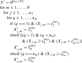(175)

where the notation $M^{[a\times b]}$ means an $a\times b$ matrix M. Notice that for bin 1 and bin $n_m$, the conditions assign data outside the RV extremes to those end bins; that is to allow variations in measured values to go under or over the extremes, but again, this may not be applicable in all situations, so modify as appropriate.

8.:

Generate the multipartite histogrammic $n\times n$ density matrix $\rho$ (where $n=n_{1}\cdots n_{N}$) using

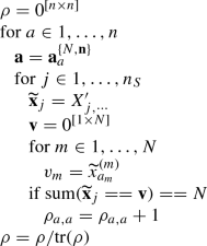(176)

where $\mathbf {a}_a^{\{ N,\mathbf {n}\} }$ is the inverse register function given in Appendix U that maps scalar index a to vector index $\mathbf {a}\equiv (a_{1},\ldots ,a_{N})$, and $\mathbf {v}\equiv (v_1,\ldots ,v_N)$ is a temporary vector to hold the multipartite representative bin value corresponding to scalar index a.

This step counts all the occurrences of each multipartite representative bin value that arises in the quantized data $X'$ and tabulates it as a relative frequency in the main diagonal of a density matrix indexed with the corresponding scalar row-column indices for that value. Note that, being diagonal by design, this $\rho$ can be stored as a vector of length n, since it is just a classical discrete probability density function, but we keep it in matrix form here for conceptual continuity with the full quantum problem.

The result of this algorithm is $\rho$, an estimator of the strictly classical density matrix, which can then be used to calculate the diagonal correlance $\mathcal {X}_D (\rho )$ in (15).

The above steps may not necessarily be the most efficient implementation of $\mathcal {A}_{\rho }$; however, in this form, the steps are at least conceptually clear.

N: Pearson correlation coefficient

Consider a system of N classical random variables (RVs) $\mathbf {x} \equiv (x^{(1)} , \ldots ,x^{(N)} )$, for a dataset X defined as a matrix of N columns representing the RVs, and $n_S$ rows each consisting of an N-tuple sample of particular measured (observed) values $\mathbf {x}_j \equiv (x_j^{(1)} , \ldots ,x_j^{(N)} )$ for the N RVs, for a total sample number of $n_S$ measured N-tuples [see (168)]. Thus, $X_{j,m}$ is the jth observed value for the mth RV $x^{(m)}$.

The sample Pearson correlation coefficient [19,20,21], which is defined only for the case of two variables, is given for any two RVs $x^{(a)}$ and $x^{(b)}$ by

$$\begin{aligned} r_{\text {P}} \equiv r_{\text {P}} ^{(a,b)} \equiv \frac{{V_S ^{(a,b)} }}{{s^{(a)} s^{(b)} }}, \end{aligned}$$

(177)

where $V_S ^{(a,b)}\equiv \text {cov}_{S}(x^{(a)},x^{(b)})$ is the (unbiased) sample covariance between $x^{(a)}$ and $x^{(b)}$,

$$\begin{aligned} \begin{array}{*{20}l} {V_S ^{(a,b)} } &{} {\equiv \frac{1}{{n_S - 1}}\sum \limits _{j = 1}^{n_S } {(x_j ^{(a)} - \mu _S^{(a)} )} (x_j ^{(b)} - \mu _S^{(b)} )} \\ {} &{} { = \frac{1}{{n_S - 1}}\sum \limits _{j = 1}^{n_S } {(X_{j,a} - \mu _S^{(a)} )} (X_{j,b} - \mu _S^{(b)} ),} \\ \end{array} \end{aligned}$$

(178)

where the sample mean of RV $x^{(m)}$ is

$$\begin{aligned} \mu _S^{(m)} \equiv \overline{x}^{(m)} \equiv \frac{1}{{n_S }}\sum \limits _{j = 1}^{n_S } {x_j^{(m)} } = \frac{1}{{n_S }}\sum \limits _{j = 1}^{n_S } {X_{j,m} } , \end{aligned}$$

(179)

and the sample standard deviation is

$$\begin{aligned} \begin{array}{*{20}l} {s^{(m)} \equiv \sqrt{V_S ^{(m,m)} } } &{} { \equiv \sqrt{\frac{1}{{n_S - 1}}\sum \limits _{j = 1}^{n_S } {(x_j ^{(m)} - \mu _S^{(m)} )^2 } } } \\ {} &{} { = \sqrt{\frac{1}{{n_S - 1}}\sum \limits _{j = 1}^{n_S } {(X_{j,m} - \mu _S^{(m)} )^2 } } .} \\ \end{array} \end{aligned}$$

(180)

We can also form an N-by-Nsample covariance matrix$V_S$ with elements $(V_S )_{a,b} \equiv V_S ^{(a,b)}$ and an N-by-Nsample Pearson correlation matrix$r_\text {P}$ with elements $(r_\text {P} )_{a,b} \equiv r_\text {P}^{(a,b)}$, each containing all pairwise covariances and Pearson correlations between the N RVs. However, it is common practice to simply write $r_{\text {P}} \equiv r_{\text {P}} ^{(a,b)}$, as in (177), to denote the scalar value of the sample Pearson correlation coefficient between two particular variables when those are the only two variables in the problem and no Pearson correlation matrix is used elsewhere in the analysis, which is the convention we use. Also, it is not standard to use the “$\text {P}$” subscript, but we use it to distinguish it from our use of r to mean rank.

The Pearson correlation has range $[-1,1]$, and is merely a measure of linear correlation between two RVs only. Thus, two variables can have strong nonlinear correlations and yet produce $r_{\text {P}}=0$, so it is not a measure of general correlation. Furthermore, the old adage that “correlation does not imply causation” means that having a nonzero $r_\text {P}$ does not mean that the RVs share some functional dependence on a common parameter, but rather it means that the data of the two RVs have a linear correspondence whether they are functions of the same underlying variables or not.

O: Consistency of strict classicality with established physics

Here, we list a few additional reasons why the strictly classical states defined in Sect. 3.3 are compatible with existing ideas in physics, and are a much more appropriate standard for classicality than coherent states.

• 1. For multiple modes of the same size, the set of all distinct pure strictly classical states has the same form as the set of possible wave functions that yield Maxwell–Boltzmann statistics [58, 59], which arise from a collection of identical but distinguishable particles and is a regime of statistics that would apply if the universe were not quantum-mechanical, i.e., in a strictly classical universe. For example, for two identical, distinguishable two-level particles, the possible wave functions are $\{ \psi _1 (x_1 ) \otimes \psi _1 (x_2 ),$$\psi _1 (x_1 ) \otimes \psi _2 (x_2 ),$$\psi _2 (x_1 ) \otimes \psi _1 (x_2 ),$$\psi _2 (x_1 ) \otimes \psi _2 (x_2 )\}$, where $\psi _a (x_m ) \equiv$$\langle x^{(m)} |\psi _a^{(m)} \rangle$, $|\psi _a^{(m)} \rangle$ is the ath possible state of particle m, and $|x^{(m)} \rangle$ is the position eigenstate of particle m. These states form a set of pure computational basis states, which qualify (in form) as strictly classical states as defined in Sect. 3.3.

• 2. In regard to probability representing the lack of knowledge of the observer, there are really two general kinds of states with different meanings [28,29,30];

  • a. Ontic states: the actual state of a system, part of fundamental reality.

  • b. Epistemic states: the state in the context of an observer, given limitations and lack of full knowledge; is usually a statistical mixture of ontic states each assigned probabilities based on observer ignorance.

  Pure strictly classical states are ontic, since the state is definite. Mixed strictly classical states are epistemic, since by the definition of strict classicality, any probability distributions arise from lack of specific knowledge (i.e., taking sample measurements with time windows too long to notice the fact that the system is instantaneously pure). This dichotomy fits nicely with the classical notion of probability; the only kind of probability in a strictly classical system is the ignorance-induced kind, and there is no fundamental quantum probability such as that which arises in pure quantum states with superposition (we exclude the possibility of hidden variable theories until Sect. 6). Furthermore, since pure strictly classical states are pure product states of computational basis states in all reference frames, nonlocal correlation is impossible in an ontic strictly classical state. In Sects. 3–5 we discuss the more interesting case of mixed strictly classical nonlocal correlation in detail.

• 3. Quantum coherence functions arise from finding mean values of quantities composed of electric field operators in analogy to classical coherence functions. What this leads to is a certification of whether or not the state of the electric field is a coherent state (which is only a necessary and sufficient certification of being in a coherent state if the field has mth-order quantum coherence values of $|g ^{(m)} (x_1 , \ldots ,x_m )| = 1$$\forall m \in \{ 1, \ldots ,\infty \}$, meaning that it is “infinite-order coherent” [27], where here $x_m\equiv (\varvec{\eta }_m,t_m)$ where $\varvec{\eta }_m \equiv \mathbf {r}-\mathbf {r}_m$ is a separation vector from source point $\mathbf {r}_m$ to field point $\mathbf {r}$ and $t_m \equiv t-\frac{|{\varvec{\eta }_m}|}{c}$ is the retarded time for light to reach $\mathbf {r}$ from $\mathbf {r}_m$).

  However, measuring how close a state is to infinite-order coherence does not prove anything about classicality; rather it is a test of how close the state is to being a coherent state (with lower-order failures such as $|g ^{(2)} (x_1 ,x_2 )| \ne 1$ being sufficient to conclude that a state is not a coherent state, thereby making such a test practical to use).

  The fallacy of assuming that a state’s classicality is determined by its similarity to a coherent state as quantified by quantum coherence functions is evident for several reasons. The main red flag indicating this fallacy is that a coherent state requires quantum superposition in the Fock basis, an impossibility in truly classical physics. Another red flag is that quantum-coherence-function results are often interpreted in conjunction with quantum-phase space probability distributions where nonclassicality is said to be evident by the appearance of negative probabilities, which are not truly allowed in quantum mechanics; a density matrix with any negative diagonal elements is nonphysical. In contrast, the definition of strict classicality forbids quantum superposition, a restriction that is a necessary requirement of classicality not satisfied by coherent states, and strict classicality requires no negative probabilities to certify it.

Regarding Reason 3 above, the classical coherence functions arise by defining abbreviations for quantities not naturally expressible in terms of electric field intensities at single spacetime points alone. The quantum coherence functions simply promote the classical field quantities to operators and promote the time average to a quantum ensemble average; thus its main claim to classicality is through a generalization of Ehrenfest’s theorem [60, 61], which is merely an approximate condition for correspondence of quantum operators to classical quantities, but not sufficient (nor exactly necessary) to determine classicality since it is not a fundamental law of quantum mechanics. In other words; even though construction of quantum coherence functions is permissible, the ability of certain quantum states (such as coherent states) to produce mean values that we expect in a classical theory is not sufficient to conclude that such states are truly classical; at best we could say that they exhibit classical behavior, and as such, coherent states might be considered the most classical of all quantum states that possess superposition in a computational basis.

P: Limits of decomposition indices

In Sect. 4.1, the decomposition unitary U is limited to dimension D of at least $r\equiv \text {rank}(\rho )$ (guaranteed by the existence of the spectral decomposition), and a minimax of at most $r^2$ (proved by P. Horodecki using the Caratheodory theorem justified by a Bloch-vector expansion [44, 62], which sets the maximum number of decomposition states needed to describe a separable state with mode-independent (MI) decomposition states [Family 5 from Table 1]), so that the number of pure decomposition states can always be limited to $D \in r, \ldots ,r^2$, even though we are free to use $D \in r, \ldots ,\infty$.

Note that in [44], the term “dimension” is used to mean “rank” which can be seen in a later work by the same author [63] in which the upper decomposition limit is clearly identified as $r^2$. The fact that this limit should be $r^2$ rather than $n^2$ is clear when we consider the case of pure states, which have $r=1$ and only need one decomposition state (the pure state itself up to global phase), regardless of dimension. However, if for some reason this interpretation is incorrect and the use of $\max (D)=r^2$ turns out to be too restrictive, then we would simply use $\max (D)=n^2$ instead. Since none of the main results in this paper rely on actually computing statance or probablance, this issue has no bearing on the main results.

Then, since $j \equiv (j_1 , \ldots ,j_N )$ is our index for decomposition states of an N-mode state, we need to determine the bounds of each $j_m$ such that we achieve a given total of D decomposition states. Therefore, if we let the range of each mode label be $j_m \in 1, \ldots ,D_m$, we can define a vector $\mathbf {D}\equiv (D_{1},\ldots ,D_{N})$ such that $D = \prod \nolimits _{m = 1}^N {D_m } = D_1 \cdots D_N$ [due to the nested sums in quantities like (24)] so that as $j \equiv (j_1 , \ldots ,j_N )$ counts over all allowed values, it has exactly D of them.

Now we just need to determine the value of a given $D_m$. By the Caratheodory theorem [44, 62], the upper necessary limit $D_m$ for each mode label for a Family-5 state is $n_{m}^2$, where $n_{m}$ is the number of levels of mode m. Thus, by this line of reasoning, we need to use

$$\begin{aligned} D_m \in 1, \ldots ,n_m ^2 \;\;\,\text {s.t.}\;\prod \limits _{m = 1}^N {D_m } = D\;\;\text {for}\;\;D \in r, \ldots ,r^2 . \end{aligned}$$

(181)

However, note that in some cases, the Caratheodory theorem’s application by P. Horodecki may be too restrictive for the following reason. Recall that in Wootters’s full concurrence paper [43], he included an explicit method showing that it is always possible to decompose any separable two-qubit state with exactly r separable decomposition states (he used n to mean rank there) of the form of Family 3 from Table 1. Yet in P. Horodecki’s paper [44], he placed an upper bound on the number of necessary separable decomposition states of $r^2$, but he used states of the form of Family 5 from Table 1, which are only a small subset of all separable states, the full set being Family 3.

The interesting thing about Wootters’s decomposition is that it also applies to the Family-5 states, meaning that even states for which statance is zero (since they have MI decomposition states) have a separable decomposition of the Family-5 form with only r members! But there is no contradiction here; the reason the Wootters decomposition works for all separable states is that it is based merely on minimizing average entanglement, a special kind of decomposition-state correlation, which means that at least for two qubits, all states with an MI set of decomposition states (Families 5 and 6 from Table 1) are guaranteed to have a separable decomposition of only r members. But because statance measures all decomposition-state correlation, of which entanglement is only a part, the decomposition that minimizes statance is generally more restrictive and therefore requires more members, so that is why we must use the Caratheodory theorem to set the limits in the statance calculation. Basically, P. Horodecki used a set of states that is only a subset of separable states; his proof applies only to Family 5 and its subset, Family 6. However, his result is still correct; it is just too loose of an upper bound for more general separable states such as those of Families 3 and 4 that are not also in Families 5 and 6.

To see how (181) fits into the decomposition of zero-statance states (since they are the standard by which zero statance is achieved), Table 3 shows all the possible decomposition vectors $\mathbf {D}$ allowable for two qubits for the purpose of keeping $D \in r,\ldots ,r^2$.

Table 3 Allowable minimally necessary numbers of two-qubit decomposition states D given $r\equiv \text {rank}(\rho )$, and vectors of possible mode-independent single-mode index limits $\mathbf {D}\equiv (D_{1},D_{2})$ such that $\prod \nolimits _{m=1}^{N}D_{m}=D$ for $D\in r,\ldots ,r^2$ as in (181)

Notice that D is never a prime number for $D> n$, and for the same reason, any numbers whose only factors include values that exceed any $n_{m}^2$ are also excluded, such as $D=10$ whose only factors are $1\cdot 10$ and $2\cdot 5$, since both 10 and 5 exceed $n_{2}^2=4$. We can use decompositions such as that, but if P. Horodecki’s proof is correct, then we are guaranteed to always be able to find a decomposition of member numbers from the set in Table 3 instead.

For example, if a decomposition for a rank-3 state is known to have 10 MI states, we should always be able to find a different MI decomposition with only $D\in \{3,4,6,8,9\}$ MI states. However, in a rank-4 state, starting with a known decomposition of 10 MI states may require that we increase to $D=12$ or $D=16$ states, depending on whether a different MI decomposition with fewer MI states than 10 exists for the input state. But if we allow things like $D=10$ here, then our single-mode limits would need to exceed the single-mode Caratheodory bounds. Therefore, the single-mode Caratheodory bounds of $n_{m}^2$ may actually lead to larger decompositions (or they may instead always allow a smaller decomposition), but we do not have a proof for the convertibility of such decompositions at this time.

To see how $\mathbf {D}$ relates to a state with zero statance, consider a two-qubit state such as

(182)

Since statance ignores the decomposition probabilities, then regardless of what they are, we can merely look at the decomposition states themselves, and here we notice that we can generate the same set from

$$\begin{aligned} \{ \rho _1^{(1)} ,\rho _2^{(1)} \} \otimes \{ \rho _1^{(2)} ,\rho _2^{(2)} ,\rho _3^{(2)} ,\rho _4^{(2)} ,\rho _5^{(2)} \} \equiv \{ \rho _{(j_1 ,j_2 )} \}, \end{aligned}$$

(183)

where the tensor product distributes over commas (if you prefer, the commas can be replaced by plus signs, and then the terms of the resulting sum comprise $\{ \rho _{(j_1 ,j_2 )} \}$. We can simplify (183) further using the notation

$$\begin{aligned} \begin{array}{*{20}l} {\{ 1,2\} \otimes \{ 1,2,3,4,5\} } &{} { \equiv \{ (j_1 ,j_2 )\} } \\ {} &{} { = \{ (1,1),(1,2),(1,3),(1,4),(1,5),} \\ {} &{}\quad {(2,1),(2,2),(2,3),(2,4),(2,5)\} .} \\ \end{array} \end{aligned}$$

(184)

The decomposition vector $\mathbf {D}\equiv (D_{1},\ldots ,D_{N})$ is a list of the maximal index labels in each mode that are needed to decompose a zero-statance state whose optimal decomposition has $D=D_{1}\cdots D_{N}$ MI decomposition states. Thus, in this example, the decomposition in (182) has

$$\begin{aligned} \mathbf {D}\equiv (2,5), \end{aligned}$$

(185)

[which are also the sizes of the mode sets in (184)]. According to P. Horodecki’s decomposition limit, which applies to states such as this, $D_2 =5$ is larger than is needed for the mode-2 limit, so we should be able to find a different decomposition with mode-2 limit $D_2 \leqslant 4$. If $r=3$, then Table 3 shows that we should be guaranteed to find such an MI decomposition of fewer members where $D\in \{3,4,6,8,9\}$, but if $r=4$, then we may or may not be able to find a different MI decomposition with fewer members, as mentioned earlier, though we are guaranteed to find one that has at most $D=r^2 =16$ MI members.

Regarding the discrepancy between Wootters’s decompositions and P. Horodecki’s limits, we may hypothesize that Wootters’s result is true for all systems (not just two qubits); that all full N-partite separable states have a decomposition of exactly r separable pure decomposition states in the form of Family 3, but that for states with zero statance, they require at least between r and $r^2$ pure decomposition states to achieve a set of MI decomposition states (and furthermore, states belonging to Families 5 and 6 all have both types of decompositions; an r-member separable decomposition, and an $(r,\ldots ,r^2)$-member zero-statance decomposition).

Note that in cases where the spectral decomposition is also a statance-minimizing decomposition, it is not necessarily $U=I^{[r]}$ that achieves this (where square bracketed superscripts indicate matrix dimension), but rather it is the r-level permutation unitary that minimizes statance. This is important when constructing examples using orthogonal decomposition states, since the descending-order convention (DOC) of eigenvalues used to define their labels does not always produce the statance-minimizing decomposition when $U=I^{[r]}$; therefore even when constructing such states, we still need to search the order of their labels to truly minimize the statance for that decomposition. Furthermore, since the eigenvalues in the probability formula $p_j = \sum \nolimits _{k = 1}^r {\lambda _k |U_{j,k} |^2 }$ in the DOC prevent any columns of U above column r from affecting the probability, the factors $|U_{j,k} |^2$ must not all be zero for a given j so that we consider only sets where $p_j > 0\;\;\forall j$. A necessary and sufficient way to ensure this is to specify that $\sum \nolimits _{k = 1}^r {|U_{j,k} |^2 } \ne 0\;\;\forall j$. Then, since there is always at least one nonzero eigenvalue, all probabilities are nonzero.

Q: Proof that statance is a necessary and sufficient measure of decomposition-state correlation

Here we prove that achieving zero statance $\hat{\mathcal {S}}(\rho )=0$ is necessary and sufficient for any mixed or pure state $\rho$ to have no decomposition-state correlation as defined in Sect. 1.1, and that having $\hat{\mathcal {S}}(\rho )>0$ is necessary and sufficient for $\rho$ to have some decomposition-state correlation, proving that statance is a necessary and sufficient measure of decomposition-state correlation.

First, the unoptimized statance $\mathcal {S}(\rho )$ of (23) has form

$$\begin{aligned} \mathcal {S}(\rho ) \equiv ||\mathbf {w}||_{1} = \sum \nolimits _{j = 1}^D {|w_j |} , \end{aligned}$$

(186)

which is just a 1-norm of the vector $\mathbf {w}$ with components

$$\begin{aligned} w_j \equiv \text {tr}[(\rho _j - \mu _j )^2 ], \end{aligned}$$

(187)

where the absolute value $|w_j |$ in (186) is because the operator $\varDelta _j\equiv \rho _j - \mu _j$ is Hermitian and therefore has only real eigenvalues, so the trace of its square as $w_j \equiv \text {tr}[\varDelta _j^2]$ in (187) is just the sum of the squares of its real eigenvalues, which is always nonnegative. Thus, it is always true that $w_j =|w_j |$. Therefore, since the necessary and sufficient condition for any 1-norm of a vector $\mathbf {w}$ to be zero is that $\mathbf {w}=\mathbf {0}$ which means that all of its components are zero $w_j =0\;\forall j$, then the necessary and sufficient condition for $\mathcal {S}(\rho )$ to be zero is that $w_j =0\;\forall j$, or equivalently, that $\rho _j =\mu _j\;\forall j$ (since that is the unique condition that causes $\rho _j - \mu _j=0$ which means that $w_j = \text {tr}[(\rho _j - \mu _j )^2] = 0\;\forall j$).

Then, due to the definition in (22) of statance $\hat{\mathcal {S}}(\rho )$ as being the minimum value of $\mathcal {S}(\rho )$ over all decompositions of $\rho$ , then the necessary and sufficient condition for $\hat{\mathcal {S}}(\rho )=0$ can be stated as

$$\begin{aligned} \hat{\mathcal {S}}(\rho ) = 0\;\;\text {iff}\;\;\exists \{ p_j ,\rho _j \} \;\;\text {s.t.}\;\;\rho _j = \mu _j \;\forall j, \end{aligned}$$

(188)

where $\{ p_j ,\rho _j \}$ is some particular decomposition set of $\rho$.

To show that statance $\hat{\mathcal {S}}(\rho )$ is a necessary and sufficient measure of decomposition-state correlation, we will first show that a sufficient condition for $\hat{\mathcal {S}}(\rho )=0$ is that $\rho$ has a decomposition with mode-independent decomposition states ($\text {MI}\{\rho _j\}$), which means that $\hat{\mathcal {S}}(\rho )=0$ is necessary for $\text {MI}\{\rho _j\}$. Then, we will show that $\hat{\mathcal {S}}(\rho )=0$ is also sufficient for $\text {MI}\{\rho _j\}$, which means that $\text {MI}\{\rho _j\}$ is necessary for $\hat{\mathcal {S}}(\rho )=0$.

To prove that having $\text {MI}\{\rho _j\}$ is sufficient for $\hat{\mathcal {S}}(\rho )=0$, we need to show that a $\rho$ with $\text {MI}\{\rho _j\}$ causes $\rho _j = \mu _j \;\forall j$. Therefore, suppose that $\rho$ has an optimal decomposition with $\text {MI}\{\rho _j\}$. Then, by definition of MI, combining (5) and (6) (using a different dummy index to keep things distinct), the decomposition states take the special form

$$\begin{aligned} \rho _j \equiv \rho _{(j_1 , \ldots ,j_N )} = \mathop \otimes \limits _{q = 1}^N \rho _{j_q }^{(q)} \;\;\forall j. \end{aligned}$$

(189)

For $\mu _j \equiv \mu _{(j_1 , \ldots ,j_N )}$ in (24), we need the quantity

$$\begin{aligned} \rho _{(j_1 ^{\{ m\} } , \ldots ,j_N ^{\{ m\} } )} = \mathop \otimes \limits _{q = 1}^N \rho _{j_q ^{\{ m\} } }^{(q)} , \end{aligned}$$

(190)

so then, the quantity

$$\begin{aligned} R_{j_m }^{(m)} \equiv \sum \limits _{j_1 ^{\{ m\} } , \ldots ,j_N ^{\{ m\} } = 1, \ldots ,1}^{D_1 , \ldots ,D_N } {\delta _{j_m ^{\{ m\} } ,j_m } \rho _{(j_1 ^{\{ m\} } , \ldots ,j_N ^{\{ m\} } )} } \end{aligned}$$

(191)

becomes

(192)

and since (24) has the form

$$\begin{aligned} \mu _j \equiv {\mathop {\otimes }\limits _{m = 1}^N} \text {tr}_{\overline{m}} \left( {\frac{1}{{D_1 \cdots D_{m - 1} D_{m + 1} \cdots D_N }}R_{j_m }^{(m)} } \right) , \end{aligned}$$

(193)

then putting (192) into (193) gives

$$\begin{aligned} \begin{array}{*{20}l} {\mu _j } &{} { = {\mathop {\otimes }\limits _{m = 1}^N} \left[ {\text {tr}\left( {\frac{1}{{D_1 }}\sum \limits _{\quad j_1 ^{\{ m\} } = 1}^{D_1 } {\rho _{j_1 ^{\{ m\} } }^{(1)} } } \right) \cdots \text {tr}\left( {\frac{1}{{D_{m - 1} }}\sum \limits _{\quad j_{m - 1} ^{\{ m\} } = 1}^{D_{m - 1} } {\rho _{j_{m - 1} ^{\{ m\} } }^{(m - 1)} } } \right) \rho _{j_m }^{(m)} } \right. } \\ {} &{} {\left. { \times \text {tr}\left( {\frac{1}{{D_{m + 1} }}\sum \limits _{\quad j_{m + 1} ^{\{ m\} } = 1}^{D_{m + 1} } {\rho _{j_{m + 1} ^{\{ m\} } }^{(m + 1)} } } \right) \cdots \text {tr}\left( {\frac{1}{{D_N }}\sum \limits _{\quad j_N ^{\{ m\} } = 1}^{D_N } {\rho _{j_N ^{\{ m\} } }^{(N)} } } \right) } \right] } { = {\mathop {\otimes }\limits _{m = 1}^N} \rho _{j_m }^{(m)} } \\ \end{array} \end{aligned}$$

(194)

and since (189) holds for each j, then (194) does as well, so then putting (194) into (189) we see that

$$\begin{aligned} \rho _j = \mu _j \;\forall j, \end{aligned}$$

(195)

which, by (188) proves that having $\text {MI}\{\rho _j\}$ is sufficient to cause $\hat{\mathcal {S}}(\rho )=0$.

To show that having $\text {MI}\{\rho _j\}$ is also necessary to cause $\hat{\mathcal {S}}(\rho )=0$, we will simply show that $\hat{\mathcal {S}}(\rho )=0$ is sufficient for $\rho$ to have $\text {MI}\{\rho _j\}$. Therefore, supposing that $\hat{\mathcal {S}}(\rho )=0$, then by (188), $\rho _j = \mu _j \;\forall j$, which by (24) is

$$\begin{aligned} \rho _{(j_1 , \ldots ,j_N )} = \mu _{(j_1 , \ldots ,j_N )} = {\mathop {\otimes }\limits _{m = 1}^N} \beta _{j_m }^{(m)} , \end{aligned}$$

(196)

where each $\beta _{j_m }^{(m)}$ is a physical state in mode m given by

$$\begin{aligned} \beta _{j_m }^{(m)} \equiv \text {tr}_{{\overline{m}}} \left( {\frac{1}{{D_{\overline{m}} }}\sum \limits _{\quad j_1 ^{\{ m\} } , \ldots ,j_{m - 1} ^{\{ m\} } ,j_{m + 1} ^{\{ m\} } , \ldots ,j_N ^{\{ m\} } = 1, \ldots ,1,1, \ldots ,1}^{{D_1 , \ldots ,D_{m - 1} ,D_{m + 1} , \ldots ,D_N }_{\qquad \qquad }} {\rho _{(j_1 ^{\{ m\} } , \ldots ,j_{m - 1} ^{\{ m\} } ,j_m ,j_{m + 1} ^{\{ m\} } , \ldots ,j_N ^{\{ m\} } )} } } \right) , \end{aligned}$$

(197)

where note that in (197) we did not expand the decomposition states further because we are making no assumption about their form in this part of the proof.

Thus, (196) shows that the condition of $\hat{\mathcal {S}}(\rho )=0$ automatically leads to a situation where the $\rho _j \equiv \rho _{(j_1 , \ldots ,j_N )}$ have a (tensor) product form of N factors guaranteed for all j, and each factor depends on a different mode-specific index $j_m$, which is the definition of the form of mode independence for decomposition states. Furthermore, since each $\beta _{j_m }^{(m)}$ is a convex sum of physical states (which are just the pure decomposition states with special mode-specific index arguments) with equal probabilities such that $\text {tr}(\beta _{j_m }^{(m)} ) = 1$, then each $\beta _{j_m }^{(m)}$ qualifies as a physical state, and we can simply rename them as states

$$\begin{aligned} \beta _{j_m }^{(m)} \equiv \rho _{j_m }^{(m)} , \end{aligned}$$

(198)

which, put into (196), is the definition of $\text {MI}\{\rho _j\}$, and so we have proven that $\hat{\mathcal {S}}(\rho )=0$ is a sufficient condition for $\text {MI}\{\rho _j\}$, and thus $\text {MI}\{\rho _j\}$ is necessary for $\hat{\mathcal {S}}(\rho )=0$.

We have now shown that the condition of a state having a decomposition with mode-independent decomposition states ($\text {MI}\{\rho _j\}$) is both necessary and sufficient to cause $\hat{\mathcal {S}}(\rho )=0$. Then, since a violation of $\text {MI}\{\rho _j\}$ implies $\hat{\mathcal {S}}(\rho )\ne 0$, and by its definition this means that $\hat{\mathcal {S}}(\rho )>0$, we have proven that statance $\hat{\mathcal {S}}(\rho )$ is a valid measure of decomposition-state correlation, since the violation of $\text {MI}\{\rho _j\}$ is the definition of decomposition-state correlation, and the achievement of $\text {MI}\{\rho _j\}$ is the necessary and sufficient condition for $\hat{\mathcal {S}}(\rho )=0$. $\square$

R: Statance example

Suppose we have a two-qubit state of the type in Family 5 of Table 1, with the statance-minimizing decomposition $\rho = \sum \nolimits _j {p_j \rho _{j_1 }^{(1)} \otimes \rho _{j_2 }^{(2)} }$, where the probabilities $p_j \equiv p_{(j_1 , j_2 )}$ in this example happen to not have mode independence, while by definition the decomposition states do have mode independence. Therefore, in this particular example, the decomposition states are

$$\begin{aligned} \begin{array}{*{20}l} {\rho _1 } &{} { \equiv \rho _{(1,1)} } &{} { = \rho _1^{(1)} \otimes \rho _1^{(2)} } \\ {\rho _2 } &{} { \equiv \rho _{(1,2)} } &{} { = \rho _1^{(1)} \otimes \rho _2^{(2)} } \\ {\rho _3 } &{} { \equiv \rho _{(2,1)} } &{} { = \rho _2^{(1)} \otimes \rho _1^{(2)} } \\ {\rho _4 } &{} { \equiv \rho _{(2,2)} } &{} { = \rho _2^{(1)} \otimes \rho _2^{(2)}. } \\ \end{array} \end{aligned}$$

(199)

To find the statance of $\rho$, first write the general form of $\mu _j \equiv \mu _{(j_1 ,j_2 )}$ from (24) with $\mathbf {D}=(2,2)$ as

$$\begin{aligned} \begin{array}{*{20}l} {\mu _j} &{} {\equiv \text {tr}_{\overline{1}} \left( {\frac{1}{2}[\rho _{(j_1 ,1)} + \rho _{(j_1 ,2)} ]} \right) \otimes \text {tr}_{\overline{2}} \left( {\frac{1}{2}[\rho _{(1,j_2 )} + \rho _{(2,j_2 )} ]} \right) .} \\ \end{array} \end{aligned}$$

(200)

Writing these out for each index and then plugging-in the particular states in (199) gives

$$\begin{aligned} \begin{array}{*{20}l} {\mu _1 } &{} { = \text {tr}_{\overline{1}} (\rho _1^{(1)} \otimes \frac{1}{2}[\rho _1^{(2)} + \rho _2^{(2)} ]) \otimes \text {tr}_{\overline{2}} (\frac{1}{2}[\rho _1^{(1)} + \rho _2^{(1)} ] \otimes \rho _1^{(2)} )} \\ {} &{} { = \rho _1^{(1)} \otimes \rho _1^{(2)} } \\ {\mu _2 } &{} { = \text {tr}_{\overline{1}} (\rho _1^{(1)} \otimes \frac{1}{2}[\rho _1^{(2)} + \rho _2^{(2)} ]) \otimes \text {tr}_{\overline{2}} (\frac{1}{2}[\rho _1^{(1)} + \rho _2^{(1)} ] \otimes \rho _2^{(2)} )} \\ {} &{} { = \rho _1^{(1)} \otimes \rho _2^{(2)} } \\ {\mu _3 } &{} { = \text {tr}_{\overline{1}} (\rho _2^{(1)} \otimes \frac{1}{2}[\rho _1^{(2)} + \rho _2^{(2)} ]) \otimes \text {tr}_{\overline{2}} (\frac{1}{2}[\rho _1^{(1)} + \rho _2^{(1)} ] \otimes \rho _1^{(2)} )} \\ {} &{} { = \rho _2^{(1)} \otimes \rho _1^{(2)} } \\ {\mu _4 } &{} { = \text {tr}_{\overline{1}} (\rho _2^{(1)} \otimes \frac{1}{2}[\rho _1^{(2)} + \rho _2^{(2)} ]) \otimes \text {tr}_{\overline{2}} (\frac{1}{2}[\rho _1^{(1)} + \rho _2^{(1)} ] \otimes \rho _2^{(2)} )} \\ {} &{} { = \rho _2^{(1)} \otimes \rho _2^{(2)} .} \\ \end{array} \end{aligned}$$

(201)

Then, putting (199) and (201) into (23), we get

$$\begin{aligned} \begin{array}{*{20}l} {\mathcal {S}(\rho )} &{} { \equiv \sum \limits _{j_1 ,j_2 =1,1}^{D_{1},D_{2}} {\text {tr}[(\rho _{(j_1 ,j_2 )} - \mu _{(j_1 ,j_2 )} )^2 ]} } \\ {} &{} { = \sum \limits _{j_1 ,j_2 =1,1}^{D_{1},D_{2}} {\text {tr}[(\rho _{j_1 }^{(1)} \otimes \rho _{j_2 }^{(2)} - \rho _{j_1 }^{(1)} \otimes \rho _{j_2 }^{(2)} )^2 ]} = 0,} \\ \end{array} \end{aligned}$$

(202)

since for this example, each $\mu _j$ is exactly equal to $\rho _j$ regardless of what the probabilities were. Then, since (202) was calculated with an optimal decomposition [because it minimizes the unoptimized statance $\mathcal {S}(\rho )$], $\mathcal {S}(\rho )$ yields the statance from (22) as

$$\begin{aligned} \hat{\mathcal {S}}(\rho ) \equiv \frac{1}{{\mathcal {N}_{\mathcal {S}} }}\mathop {\min }\limits _{\{ U\} } [\mathcal {S}(\rho )] = 0. \end{aligned}$$

(203)

Thus, this example shows that any states belonging to Families 5 or 6 from Table 1 have zero statance regardless of their decomposition probabilities, because those states all have mode-independent sets of decomposition states for their statance-minimizing decompositions.

S: Proof that probablance is a necessary and sufficient measure of probability correlation

Here we prove that achieving zero probablance $\hat{\mathcal {P}}(\rho )=0$ is necessary and sufficient for any mixed or pure state $\rho$ to have no probability correlation as defined in Sect. 1.1, and that having $\hat{\mathcal {P}}(\rho )>0$ is necessary and sufficient for the state to have some probability correlation, proving that probablance is a necessary and sufficient measure of probability correlation.

First, note that the unoptimized probablance $\mathcal {P}(\rho )$ from (27) can be written as

$$\begin{aligned} \mathcal {P}(\rho ) \equiv |\mathbf {v}|^2 = \sum \nolimits _j {|v_j |^2 } , \end{aligned}$$

(204)

which is just a nonzero scalar times a 2-norm of the vector

$$\begin{aligned} \mathbf {v}\equiv \mathbf {p}^{\prime }-\mathbf {q}^{\prime }, \end{aligned}$$

(205)

where $\mathbf {p}^{\prime }$ has components $p_j^{\prime } \equiv p_{(j_1 , \ldots ,j_N )}^{\prime }$ which is the set of decomposition probabilities of an arbitrary statance-minimizing (SM) decomposition of $\rho$ as given by (29), and $\mathbf {q}^{\prime }$ has components $q_j^{\prime } \equiv q_{(j_1 , \ldots ,j_N )}^{\prime }$ defined in (28), so $\mathbf {v}$ has components $v_j \equiv p_j^{\prime } - q_j^{\prime }$. Therefore, since the necessary and sufficient condition for any 2-norm of a vector $\mathbf {v}$ to be zero is that $\mathbf {v}=\mathbf {0}$, which means that all of its components are zero $v_j \equiv 0\;\forall j$, then the necessary and sufficient condition for $\mathcal {P}(\rho )$ to be zero is that $v_j \equiv 0\;\forall j$, or equivalently, that $p_j^{\prime } = q_j^{\prime } \;\forall j$. Then, due to the definition in (26) of $\hat{\mathcal {P}}(\rho )$ as being the minimum value of $\mathcal {P}(\rho )$ over all SM decompositions of $\rho$, the necessary and sufficient condition for $\hat{\mathcal {P}}(\rho )=0$ can be stated as

$$\begin{aligned} \hat{\mathcal {P}}(\rho ) = 0 \; \;\text{ iff }\;\; \exists \{ p_j^{\prime } , \rho _j^{\prime }\} \;\;\text{ s.t. }\; \;p_j^{\prime } = q_j^{\prime } \; \forall j\;\;\text{ and }\;\;\hat{\mathcal {S}}(\rho )= \hat{\mathcal {S}}_{\min }, \end{aligned}$$

(206)

where $\{ p_j^{\prime } ,\rho _j^{\prime } \}$ is some particular SM decomposition of $\rho$, $\hat{\mathcal {S}}(\rho )$ is the statance from Sect. 4.1, and $\hat{\mathcal {S}}_{\min }$ is the minimal $\hat{\mathcal {S}}(\rho )$ over all decompositions of $\rho$. (The requirement that $\{ p_j^{\prime } ,\rho _j^{\prime } \}$ causes $\hat{\mathcal {S}}_{\min }$ is actually already part of the definition of $\{ p_j^{\prime } ,\rho _j^{\prime } \}$, so it is redundant in (206), but stated anyway to emphasize its importance).

To show that $\hat{\mathcal {P}}(\rho )$ is a necessary and sufficient measure of probability correlation, we will first show that a sufficient condition for $\hat{\mathcal {P}}(\rho )=0$ is that $\rho$ has an SM decomposition with mode-independent probabilities ($\text {MI}\{p_{j}\}_{\text {SM}}\equiv \text {MI}\{p_{j}^{\prime }\}$), meaning that $\hat{\mathcal {P}}(\rho )=0$ is necessary for $\text {MI}\{p_{j}\}_{\text {SM}}$. Then, we will show that $\hat{\mathcal {P}}(\rho )=0$ is also sufficient for $\text {MI}\{p_{j}\}_{\text {SM}}$, meaning that $\text {MI}\{p_{j}\}_{\text {SM}}$ is also necessary for $\hat{\mathcal {P}}(\rho )=0$.

To prove that having $\text {MI}\{p_{j}\}_{\text {SM}}$ is sufficient for $\hat{\mathcal {P}}(\rho )=0$, we need to show that a state $\rho$ with $\text {MI}\{p_{j}\}_{\text {SM}}$ causes $p_j^{\prime } = q_j^{\prime } \;\forall j$. Therefore, suppose that $\rho$ has an SM decomposition with $\text {MI}\{p_{j}\}_{\text {SM}}$. Then, by definition, combining (7) and (8) (using a different dummy index to keep things distinct),

$$\begin{aligned} p_j^{\prime } \equiv p_{(j_1 , \ldots ,j_N )}^{\prime } = \prod \nolimits _{q = 1}^N p_{j_q }^{(q)} \;\;\forall j, \end{aligned}$$

(207)

where $\sum \nolimits _{j_q } {p_{j_q }^{(q)} } = 1;\;\;\forall q \in 1, \ldots ,N$. For $q_j^{\prime } \equiv q_{(j_1 , \ldots ,j_N )}^{\prime }$ in (28), we need the quantity

$$\begin{aligned} p_{(j_1 ^{\{ m\} } , \ldots ,j_N ^{\{ m\} } )}^{\prime } = \prod \nolimits _{q = 1}^N p_{j_q ^{\{ m\} } }^{(q)} , \end{aligned}$$

(208)

so then, the quantity

$$\begin{aligned} Q_{j_m }^{(m)} \equiv \sum \limits _{j_1 ^{\{ m\} } , \ldots ,j_N ^{\{ m\} }= 1, \ldots ,1 }^{D_1 , \ldots ,D_N } {\delta _{j_m ^{\{ m\} } ,j_m } p_{(j_1 ^{\{ m\} } , \ldots ,j_N ^{\{ m\} } )}^{\prime } } \end{aligned}$$

(209)

takes on the value

$$\begin{aligned} \begin{array}{*{20}l} {Q_{j_m }^{(m)} } &{} { = \sum \limits _{\qquad j_1 ^{\{ m\} } , \ldots ,j_N ^{\{ m\} }= 1, \ldots ,1 }^{D_1 , \ldots ,D_N } {\delta _{j_m ^{\{ m\} } ,j_m } \prod \nolimits _{q = 1}^N {p_{j_q ^{\{ m\} } }^{(q)} } } } \\ {} &{} { = \qquad \sum \limits _{\qquad j_1 ^{\{ m\} } , \ldots ,j_{m - 1} ^{\{ m\} } ,j_{m + 1} ^{\{ m\} } , \ldots ,j_N ^{\{ m\} } = 1, \ldots ,1,1, \ldots ,1}^{{D_1 , \ldots ,D_{m - 1} ,D_{m + 1} , \ldots ,D_N }_{\qquad \qquad }} {p_{j_1 ^{\{ m\} } }^{(1)} \cdots p_{j_{m - 1} ^{\{ m\} } }^{(m - 1)} p_{j_m }^{(m)} p_{j_{m + 1} ^{\{ m\} } }^{(m + 1)} \cdots p_{j_N ^{\{ m\} } }^{(N)} } } \\ {} &{} { = \left[ {\left( {\sum \limits _{j_1 ^{\{ m\} } =1}^{D_{1}} {p_{j_1 ^{\{ m\} } }^{(1)} } }\right) \cdots \left( {\sum \limits _{j_{m - 1} ^{\{ m\} } =1}^{D_{m-1}} {p_{j_{m - 1} ^{\{ m\} } }^{(m - 1)} } }\right) p_{j_m }^{(m)} } \right. } {\left. { \left( {\sum \limits _{j_{m + 1} ^{\{ m\} } =1}^{D_{m+1}} {p_{j_{m + 1} ^{\{ m\} } }^{(m + 1)} } }\right) \cdots \left( {\sum \limits _{j_N ^{\{ m\} } =1}^{D_{N}} {p_{j_N ^{\{ m\} } }^{(N)} } }\right) } \right] } \\ {} &{} { = p_{j_m }^{(m)} ,} \\ \end{array}\nonumber \\ \end{aligned}$$

(210)

which, when put into (28), gives

$$\begin{aligned} q_j^{\prime } \equiv q_{(j_1 , \ldots ,j_N )}^{\prime } = \prod \nolimits _{m = 1}^N p_{j_m }^{(m)} . \end{aligned}$$

(211)

Since (207) holds for each j, then (211) does as well, so then putting (211) into (207), we see that

$$\begin{aligned} p_j^{\prime } = q_j^{\prime } \;\forall j, \end{aligned}$$

(212)

which, by (206) proves that having $\text {MI}\{p_{j}\}_{\text {SM}}$ is sufficient to cause $\hat{\mathcal {P}}(\rho )=0$.

To show that having $\text {MI}\{p_{j}\}_{\text {SM}}$ is also necessary to cause $\hat{\mathcal {P}}(\rho )=0$, we will simply show that $\hat{\mathcal {P}}(\rho )=0$ is sufficient for $\rho$ to have $\text {MI}\{p_{j}\}_{\text {SM}}$. Therefore, supposing that $\hat{\mathcal {P}}(\rho )=0$, then by (204) and (205), $p_j^{\prime } = q_j^{\prime } \;\forall j$, which expands using (28) as

$$\begin{aligned} p_{(j_1 , \ldots ,j_N )}^{\prime } = \prod \nolimits _{m = 1}^N {b_{j_m }^{(m)} } , \end{aligned}$$

(213)

where we define the quantity

$$\begin{aligned} b_{j_m }^{(m)} \equiv \sum \limits _{\qquad j_1 ^{\{ m\} } , \ldots ,j_{m - 1} ^{\{ m\} } ,j_{m + 1} ^{\{ m\} } , \ldots ,j_N ^{\{ m\} } = 1, \ldots ,1,1, \ldots ,1}^{{D_1 , \ldots ,D_{m - 1} ,D_{m + 1} , \ldots ,D_N }_{\qquad \qquad }} {p_{(j_1 ^{\{ m\} } , \ldots ,j_{m - 1} ^{\{ m\} } ,j_m ,j_{m + 1} ^{\{ m\} } , \ldots ,j_N ^{\{ m\} } )}^{\prime } } , \end{aligned}$$

(214)

where we cannot simplify the probabilities further because we are making no assumptions about their form here. Also, since the sum of all the $p_j^{\prime } \equiv p_{(j_1 , \ldots ,j_N )}^{\prime }$ is 1, and the sum in (214) is missing one of the mode sums that would complete that sum to 1, and since the terms in (214) are all probabilities existing on [0, 1], then these quantities $b_{j_m }^{(m)}$ generally satisfy

$$\begin{aligned} 0 \leqslant b_{j_m }^{(m)} \leqslant 1. \end{aligned}$$

(215)

Thus, (213) shows that the condition of $\hat{\mathcal {P}}(\rho )=0$ automatically leads to a situation where each $p_j^{\prime } \equiv p_{(j_1 , \ldots ,j_N )}^{\prime }$ has a product form of N factors guaranteed for all j, and each factor depends on a different mode-specific index $j_m$, which is the definition of the form of mode independence. Furthermore, since $b_{j_m }^{(m)} \in [0,1]$ by (215), then by the normalization property of the $p_j^{\prime } \equiv p_{(j_1 , \ldots ,j_N )}^{\prime }$, the mode-independence leads to all the sums producing positive factors, seen by summing (213) as

$$\begin{aligned} \begin{array}{*{20}l} {\sum \limits _{j_1 , \ldots ,j_N = 1, \ldots ,1}^{D_1 , \ldots ,D_N } {p_{(j_1 , \ldots ,j_N )} } } &{} { = \left( {\sum \limits _{j_1 =1}^{D_{1}} {b_{j_1 }^{(1)} } }\right) \cdots \left( {\sum \limits _{j_N =1}^{D_{N}} {b_{j_N }^{(N)} } }\right) } \\ {1} &{} { = B^{(1)} \cdots B^{(N)} ,} \\ \end{array} \end{aligned}$$

(216)

where $B^{(m)} \equiv \sum \nolimits _{j_m } {b_{j_m }^{(m)} }$ such that $B^{(m)} \in [0,1]$. Then, the only way that the right-side product, with each factor on [0, 1], could equal the left is if all of the factors are 1, meaning $B^{(m)} =1\;\forall m$, which means that each $b_{j_m }^{(m)}$ then satisfies all of the conditions for being a probability since $b_{j_m }^{(m)} \in [0,1]$ and $\sum \nolimits _{j_m } {b_{j_m }^{(m)} }=1$. [Also, $\sum \nolimits _{j_m } {b_{j_m }^{(m)} }=1$due to the definition in (214) because it supplies the missing mode sum for the full probabilities to sum to 1.] Therefore, we can rename them as mode-specific probabilities

$$\begin{aligned} b_{j_m }^{(m)} \equiv p_{j_m }^{(m)} , \end{aligned}$$

(217)

obeying $\sum \nolimits _{j_m } {p_{j_m }^{(m)} }=1$ so that (213) becomes

$$\begin{aligned} p_{(j_1 , \ldots ,j_N )}^{\prime } = \prod \nolimits _{m = 1}^N {p_{j_m }^{(m)} };\;\;\sum \nolimits _{j_m } {p_{j_m }^{(m)} }=1\;\;\forall m \;\forall j , \end{aligned}$$

(218)

which is the definition of $\text {MI}\{p_{j}\}_{\text {SM}}$, and therefore we have proven that $\hat{\mathcal {P}}(\rho )=0$ is a sufficient condition for $\text {MI}\{p_{j}\}_{\text {SM}}$, and thus $\text {MI}\{p_{j}\}_{\text {SM}}$ is necessary for $\hat{\mathcal {P}}(\rho )=0$.

We have now shown that the condition of a state having an SM decomposition with mode-independent decomposition probabilities ($\text {MI}\{p_{j}\}$) is both necessary and sufficient to cause $\hat{\mathcal {P}}(\rho )=0$. Then, since a violation of $\text {MI}\{p_{j}\}_{\text {SM}}$ implies $\hat{\mathcal {P}}(\rho )\ne 0$, and by its definition this means that $\hat{\mathcal {P}}(\rho )> 0$, we have proven that probablance $\hat{\mathcal {P}}(\rho )$ is a valid measure of probability correlation, since violation of $\text {MI}\{p_{j}\}_{\text {SM}}$ is the definition of probability correlation, and achievement of $\text {MI}\{p_{j}\}_{\text {SM}}$ is the necessary and sufficient condition for $\hat{\mathcal {P}}(\rho )=0$. See Sect. 4.2 for the explanation of why we must use a statance-minimizing decomposition to compute probablance. $\square$

T: Probablance example

To see how probablance works for a state with mode-independent (MI) probabilities of a statance-minimizing (SM) decomposition, consider the special case of some product-form two-qubit input mixed state $\rho$, which, due to its product form, has an optimal decomposition [one that minimizes the unoptimized probablance of (27)] with probabilities of the form

$$\begin{aligned} \begin{array}{*{20}l} {p_{(1,1)}^{\prime } } &{} { = p_1^{(1)} p_1^{(2)} } \\ {p_{(1,2)}^{\prime } } &{} { = p_1^{(1)} p_2^{(2)} } \\ {p_{(2,1)}^{\prime } } &{} { = p_2^{(1)} p_1^{(2)} } \\ {p_{(2,2)}^{\prime } } &{} { = p_2^{(1)} p_2^{(2)}, } \\ \end{array} \end{aligned}$$

(219)

where $p_1^{(m)} + p_2^{(m)} = 1$, and these $p_{(j_1 , \ldots ,j_N )}^{\prime }$ are found from solving the optimization problem over all the unitaries $U^{\prime }$ of an SM decomposition that produce $p_{(j_1 , \ldots ,j_N )}^{\prime }$ from (29) to minimize $\mathcal {P}(\rho )$ in (27) to give the probablance $\hat{\mathcal {P}}(\rho )$ in (26). (In practice, we would just get a list of numbers that have this structure, but we would not know it at this point in the calculation; it would only be clear when we finish computing the probablance.)

In Appendix E we proved that any mixed product-form state has an optimal decomposition of $r=\text {rank}(\rho )$ decomposition states, where the rank of each single-mode reduction is $r_m$ and $r_1 \cdots r_N = r$. Using this fact, then $\mathbf {D}=(2,2)$, and the overall form of $q_{j}^{\prime }$ from (28) is

$$\begin{aligned} q_{(j_1 ,j_2 )}^{\prime }=(p_{(j_1 ,1)}^{\prime } + p_{(j_1 ,2)}^{\prime } )(p_{(1,j_2 )}^{\prime } + p_{(2,j_2 )}^{\prime } ). \end{aligned}$$

(220)

Then, using the particular values of (219) in (220) gives

$$\begin{aligned} \begin{array}{*{20}l} {q_{(1,1)}^{\prime } } &{} { = (p_1^{(1)} p_1^{(2)} + p_1^{(1)} p_2^{(2)} )(p_1^{(1)} p_1^{(2)} + p_2^{(1)} p_1^{(2)} )} \\ {} &{} { = p_1^{(1)} (p_1^{(2)} + p_2^{(2)} )(p_1^{(1)} + p_2^{(1)} )p_1^{(2)} } \\ {} &{} { = p_1^{(1)} p_1^{(2)}, } \\ \end{array} \end{aligned}$$

(221)

and similarly,

$$\begin{aligned} \begin{array}{*{20}l} {q_{(1,2)}^{\prime } } &{} { = (p_1^{(1)} p_1^{(2)} + p_1^{(1)} p_2^{(2)} )(p_1^{(1)} p_2^{(2)} + p_2^{(1)} p_2^{(2)} )} &{} { = p_1^{(1)} p_2^{(2)} } \\ {q_{(2,1)}^{\prime } } &{} { = (p_2^{(1)} p_1^{(2)} + p_2^{(1)} p_2^{(2)} )(p_1^{(1)} p_1^{(2)} + p_2^{(1)} p_1^{(2)} )} &{} { = p_2^{(1)} p_1^{(2)} } \\ {q_{(2,2)}^{\prime } } &{} { = (p_2^{(1)} p_1^{(2)} + p_2^{(1)} p_2^{(2)} )(p_1^{(1)} p_2^{(2)} + p_2^{(1)} p_2^{(2)} )} &{} { = p_2^{(1)} p_2^{(2)} ,} \\ \end{array} \end{aligned}$$

(222)

which are exactly the same as the optimal decomposition probabilities themselves [which only happens when the optimal decomposition probabilities have mode independence as in (219)]. Thus, putting (221–222) into (27),

$$\begin{aligned} \mathcal {P}(\rho ) = \sum \limits _{j_1 ,j_2 =1,1}^{D_{1},D_{2}} {|p_{(j_1 ,j_2 )}^{\prime } - q_{(j_1 ,j_2 )}^{\prime } |^2 } = 0, \end{aligned}$$

(223)

which also yields the fully optimized probablance as $\hat{\mathcal {P}}(\rho )=0$ here, since we specified that the $U^{\prime }$ we used to get the $p_{(j_1 ,j_2 )}^{\prime }$ produced an SM decomposition, and since 0 is the lowest value that $\mathcal {P}(\rho )$ can have, then this decomposition minimizes the unoptimized probablance.

Thus, this example shows the mechanism by which states with SM decompositions of mode-independent product-form probabilities produce a probablance of 0.

U: Register and inverse register functions

Register counting is any ordered set of sets of characters for which the rightmost character increases in its ordered set until it reaches the end, and then the character to its immediate left can increment by one member in its ordered set, but the character to its right simultaneously resets and must go through another cycle before the character to its left can increment again.

For example, in a two-character word where each character has an alphabet of two letters (a system with structure $2\times 2$ such as two qubits), register counting goes as $\{(1,1),(1,2),(2,1),(2,2)\}$. We can relabel this vector-index list with the scalar-index labels $\{1,2,3,4\}$.

For an N-mode discrete quantum system with structure $\mathbf {n}=(n_1 ,\ldots ,n_{N})$, where mode m has $n_m$ outcomes labeled in increasing order from 1 to $n_m$, the map from a particular vector-index outcome labeled as $\mathbf {a}=(a_1 ,\ldots ,a_{N})$, where $a_m \in 1, \ldots ,n_m \;\forall m\in 1,\ldots ,N$ to the scalar-index outcome in the set $1,\ldots ,n$, where $n\equiv n_{1}\cdots n_N$, is given by the indical register function [18, 47],

$$\begin{aligned} \begin{array}{*{20}l} {R_\mathbf {a}^{\{ N,\mathbf {n}\} } } &{} { \equiv 1 + \sum \limits _{m = 1}^N {\left( {(a_m - 1)\prod \limits _{j = m + 1}^N {n_j } } \right) }} \\ {} &{} { = (a_1 - 1)(n_2 \cdots n_N ) + (a_2 - 1)(n_3 \cdots n_N ) + \cdots } \\ {} &{} {\;\;\;\, + (a_{N - 2} - 1)(n_{N - 1} n_N ) + (a_{N - 1} - 1)n_N + a_N ,} \\ \end{array} \end{aligned}$$

(224)

which maps the vector index $\mathbf {a}$ to scalar index a as $a=R_\mathbf {a}^{\{ N,\mathbf {n}\} }$. For example, in a two-qubit system, for which $\mathbf {n}=(2,2)$, (224) maps the vector index (2, 1) to the scalar index 3.

In other situations, we know a scalar-index value a and want to know to which vector-index $\mathbf {a}$ it corresponds. For that, we use the inverse indical register function [18],

$$\begin{aligned} \mathbf {a}_a^{\{ N,\mathbf {n}\} } = (a_1 , \ldots a_N );\;\;\left\{ {\begin{array}{*{20}l} {a_m } &{} { = \text {floor}\left( \frac{v_{m - 1} - 1}{d_{m}}\right) +1} \\ {v_m } &{} { = v_{m - 1} - (a_m - 1)d_m ,} \\ \end{array}} \right. \end{aligned}$$

(225)

for $m\in 1,\ldots ,N$, where $v_0 \equiv a$, and $d_m \equiv \varPi _{q=m+1}^{N}n_{q}$. Thus (225) maps scalar index a to vector index $\mathbf {a}$ as $\mathbf {a}=\mathbf {a}_a^{\{ N,\mathbf {n}\} }$. For example, in a two-qubit system, (225) maps scalar index 2 to vector index (1, 2).

Note that throughout this paper, although $\mathbf {n}$ is the mode-size vector to use for register counting of the basis functions with (224) and (225), in the case of register counting the decomposition indices$j\equiv (j_{1},\ldots ,j_{N})$, we need to use the decomposition-limit vector $\mathbf {D}\equiv (D_{1},\ldots ,D_{N})$ [see Appendix P] instead of $\mathbf {n}$ in (224) and (225) to convert between scalar decomposition indices j and vector decomposition indices $(j_{1},\ldots ,j_{N})$ [where again all indices start on 1]. Thus we have $j=R_\mathbf {j}^{\{ N,\mathbf {D}\} }$ and $\mathbf {j}=\mathbf {j}_j^{\{ N,\mathbf {D}\} }$, where $n_m \rightarrow D_m$, $a_m \rightarrow j_m$, $v_0 \equiv j$, and we use $\mathbf {j}$ to specifically mean the vector index as a collection of many indices $\mathbf {j}\equiv (j_{1},\ldots ,j_{N})$ rather than as a single equivalent number j.

References

Feynman, R.P.: Quantum mechanical computers. Found. Phys. 16, 507 (1986)
DiVincenzo, D.P.: The physical implementation of quantum computation (2000). arXiv:quant-ph/0002077
Bennett, C.H., Brassard, G.: Quantum cryptography: public key distribution and coin tossing. In: Proceedings of IEEE International Conference on Computers, Systems and Signal Processing, vol. 175 (1984)
Bennett, C.H.: Quantum cryptography using any two nonorthogonal states. Phys. Rev. Lett. 68, 3121 (1992)
Ekert, A.K.: Quantum cryptography based on Bell’s theorem. Phys. Rev. Lett. 67, 661 (1991)
Bennett, C.H., Brassard, G., Crépeau, C., Jozsa, R., Peres, A., Wootters, W.K.: Teleporting an unknown quantum state via dual classical and Einstein–Podolsky–Rosen channels. Phys. Rev. Lett. 70, 1895 (1993)
Bouwmeester, D., Pan, J.W., Mattle, K., Eibl, M., Weinfurter, H., Zeilinger, A.: Experimental quantum teleportation. Nature 390, 575 (1997)
Bouwmeester, D., Pan, J.W., Mattle, K., Eibl, M., Weinfurter, H., Zeilinger, A.: Experimental quantum teleportation. Philos. Trans. R. Soc. Lond. A 356, 1733 (1998)
Hedemann, S.R.: Noise-resistant quantum teleportation, ansibles, and the no-projector theorem (2016). arXiv:1605.09233
Nielsen, M.A., Chuang, I.L.: Quantum Computation and Quantum Information. Cambridge University Press, Cambridge (2010)
Ollivier, H., Zurek, W.H.: Quantum discord: a measure of the quantumness of correlations. Phys. Rev. Lett. 88, 017901 (2001)
Henderson, L., Vedral, V.: Classical, quantum and total correlations. J. Phys. A 34, 6899 (2001)
Ali, M., Rau, A.R.P., Alber, G.: Quantum discord for two-qubit X states. Phys. Rev. A 81, 042105 (2010)
Bennett, C.H., DiVincenzo, D.P., Fuchs, C.A., Mor, T., Rains, E., Shor, P.W., Smolin, J.A., Wootters, W.K.: Quantum nonlocality without entanglement. Phys. Rev. A 59, 1070 (1999)
Horodecki, M., Horodecki, P., Horodecki, R., Oppenheim, J., Sen, A., Sen, U., Synak-Radtke, B.: Local versus non-local information in quantum information theory: formalism and phenomena. Phys. Rev. A 71, 062307 (2005)
Niset, J., Cerf, N.J.: Multipartite nonlocality without entanglement in many dimensions. Phys. Rev. A 74, 052103 (2006)
Hedemann, S.R.: Evidence that all states are unitarily equivalent to X states of the same entanglement (2013). arXiv:1310.7038
Hedemann, S.R.: Ent: A multipartite entanglement measure, and parameterization of entangled states. Quant. Inf. Comput. 18, 389 (2018). arXiv:1611.03882
Galton, F.: Typical laws of heredity. Nature 15, 512 (1877)
Pearson, K.: Notes on regression and inheritance in the case of two parents. Proc. R. Soc. Lond. 58, 240 (1895)
Devore, J.L.: Probability and Statistics for Engineering and the Sciences, 6th edn. Brooks/Cole, Pacific Grove (2004)
Hedemann, S.R.: Candidates for universal measures of multipartite entanglement. Quant. Inf. Comput. 18, 443 (2018). arXiv:1701.03782
Dirac, P.A.M.: The quantum theory of the emission and absorption of radiation. Proc. R. Soc. A 114, 243 (1927)
Glauber, R.J.: The quantum theory of optical coherence. Phys. Rev. 130, 2529 (1963)
Glauber, R.J.: Coherent and incoherent states of the radiation field. Phys. Rev. 131, 2766 (1963)
Titulaer, U.M., Glauber, R.J.: Correlation functions for coherent fields. Phys. Rev. 140, B676 (1965)
Gerry, C.C., Knight, P.L.: Introductory Quantum Optics, pp. 120–130. Cambridge University Press, Cambridge (2005)
Spekkens, R.W.: In defense of the epistemic view of quantum states: a toy theory. Phys. Rev. A 75, 032110 (2007)
Pusey, M.F., Barrett, J., Rudolph, T.: On the reality of the quantum state. Nature 8, 475 (2012)
Harrigan, N., Spekkens, R.W.: Einstein, incompleteness, and the epistemic view of quantum states. Found. Phys. 40, 125 (2010)
Hedemann, S.R.: Hyperspherical parameterization of unitary matrices (2013). arXiv:1303.5904
Werner, R.F.: Quantum states with Einstein–Podolsky–Rosen correlations admitting a hidden-variable model. Phys. Rev. A 40, 4277 (1989)
Bacciagaluppi, G., Valentini, A.: Quantum Theory at the Crossroads: Reconsidering the 1927 Solvay Conference, p. 175. Cambridge University Press, Cambridge (2009)
Einstein, A., Podolsky, B., Rosen, N.: Can quantum-mechanical description of reality be considered complete? Phys. Rev. 47, 777 (1935)
Einstein, A.: Physics and reality. J. Frankl. Inst. 221, 313–349 (1936)
Bell, J.S.: On the Einstein Podolsky Rosen paradox. Physics 1, 195 (1964)
Clauser, J.F., Horne, M.A., Shimony, A., Holt, R.A.: Proposed experiment to test local hidden-variable theories. Phys. Rev. Lett. 23, 880 (1969)
Aspect, A., Dalibard, J., Roger, G.: Experimental test of Bell’s Inequalities using time-varying analyzers. Phys. Rev. Lett. 49, 1804 (1982)
Greenberger, D.M., Horne, M., Zeilinger, A.: Bell’s theorem, quantum theory, and conceptions of the universe. In: Kafatos, M. (ed.) Kluwer, Dordrecht (1989)
Greenberger, D.M., Horne, M., Shimony, A., Zeilinger, A.: Bell’s theorem without inequalities. Am. J. Phys. 58, 1131 (1990)
Mermin, N.D.: What’s wrong with these elements of reality? Phys. Today 43, 9 (1990)
Hill, S., Wootters, W.K.: Entanglement of a pair of quantum bits. Phys. Rev. Lett. 78, 5022 (1997)
Wootters, W.K.: Entanglement of formation of an arbitrary state of two qubits. Phys. Rev. Lett. 80, 2245 (1998)
Horodecki, P.: Separability criterion and inseparable mixed states with positive partial transposition. Phys. Lett. A 232, 333 (1997)
Horodecki, P., Horodecki, M., Horodecki, R.: Bound entanglement can be activated. Phys. Rev. Lett. 82, 1056 (1999)
Horodecki, M., Horodecki, P., Horodecki, R.: Mixed-state entanglement and distillation: Is there a “bound” entanglement in nature? Phys. Rev. Lett. 80, 5239 (1998)
Hedemann, S.R.: Hyperspherical Bloch vectors with applications to entanglement and quantum state tomography. Ph.D. thesis, Stevens Institute of Technology. UMI Diss. Pub. 3636036 (2014)
Mendonça, P.E.M.F., Marchiolli, M.A., Galetti, D.: Entanglement universality of two-qubit X-states. Ann. Phys. 351, 79 (2014)
Mendonça, P.E.M.F., Marchiolli, M.A., Hedemann, S.R.: Maximally entangled mixed states for qubit-qutrit systems. Phys. Rev. A 95, 022324 (2017)
Hedemann, S.R.: X states of the same spectrum and entanglement as all two-qubit states. Quant. Inf. Process. 17, 293 (2018). arXiv:1802.03038
Streltsov, A., Kampermann, H., Bru, D.: Linking a distance measure of entanglement to its convex roof. New J. Phys. 12, 123004 (2010)
Bloch, F.: Nuclear induction. Phys. Rev. 70, 460 (1946)
Stokes, G.G.: On the composition and resolution of streams of polarized light from different sources. Trans. Camb. Philos. Soc. 9, 399 (1852)
von Neumann, J.: Mathematische begründung der quantenmechanik. (German) [The mathematical basis of quantum mechanics]; Wahrscheinlichkeitstheoretischer aufbau der quantenmechanik. (German) [Probabilistic structure of quantum mechanics]. Göttinger Nachrichten, 1, 245 (1927)
Ne’eman, Y.: Derivation of strong interactions from a gauge invariance. Nucl. Phys. 26, 222 (1961)
Gell-Mann, M.: Symmetries of baryons and mesons. Phys. Rev. 125, 1067 (1962)
Hioe, F.T., Eberly, J.H.: N-level coherence vector and higher conservation laws in quantum optics and quantum mechanics. Phys. Rev. Lett. 47, 838 (1981)
Sakurai, J.J.: Modern quantum mechanics revised edition. In: Tuan, S.F. (ed.) Addison-Wesley Publishing Company, Inc., p. 362 (1994)
Reif, F.: Fundamentals of Statistical and Thermal Physics, pp. 331–333. Waveland Press Inc, Long Grove (2009)
Ehrenfest, P.: Bemerkung über die angenäherte gültigkeit der klassischen mechanik innerhalb der quantenmechanik (German). Zeitschrift für Physik 45, 455 (1927)
Griffiths, D.J.: Introduction to Quantum Mechanics, 2nd edn, p. 18,115. Pearson Education Inc, Boston (2005)
Carathéodory, C.: Über den variabilitätsbereich der Koeffizienten von Potenzreihen, die gegebene werte nicht annehmen (German). Mathematische Annalen 64, 95 (1907)
Horodecki, P., Smolin, J.A., Terhal, B.M., Thapliyal, A.V.: Rank two bipartite bound entangled states do not exist. Theor. Comput. Sci. 292, 589 (2003)
Author information
Authors and Affiliations
Corresponding author
Ethics declarations
Conflict of interest
The author declares that he has no conflict of interest.
Additional information
Publisher's Note
Springer Nature remains neutral with regard to jurisdictional claims in published maps and institutional affiliations.