Article

Exploration of Seafloor Massive Sulfide Deposits with Fixed-Offset Marine Controlled Source Electromagnetic Method: Numerical Simulations and the Effects of Electrical Anisotropy

1
Institute of Geophysics and Geomatics, China University of Geosciences, Wuhan 430074, China
2
Geological Survey, China University of Geosciences, Wuhan 430074, China
*
Authors to whom correspondence should be addressed.
Minerals 2020, 10(5), 457; https://doi.org/10.3390/min10050457
Submission received: 31 March 2020 / Revised: 6 May 2020 / Accepted: 15 May 2020 / Published: 19 May 2020
(This article belongs to the Special Issue Marine Geology and Minerals)

Abstract

:
Seafloor massive sulfide (SMS) deposits have attracted growing interest and become the focus of current seafloor mineral exploration. One key challenge is to delineate potential SMS accumulations and estimate their quantity and quality for prospective resource mining. Recently, geophysical electromagnetic methods which are routinely used for land-based mineral exploration are being adapted to detect and assess SMS occurrences by imaging their conductivity distributions. However, the rough seafloor topography and electrical anisotropy of the seafloor formations encountered in practical surveys pose challenges for reliable data interpretation, and recent studies have revealed that the rough bathymetry could cause measurable distortions. Here, we consider a fixed-offset marine controlled-source electromagnetic method (CSEM) for SMS exploration, and investigate the effects of electrical anisotropy of sedimentary formations through numerical simulations for marine CSEM surveys aiming at conductive targets in the shallow regions of the seafloor. Numerical results demonstrate that the presence of electrical anisotropy could impose significant influence on fixed-offset marine CSEM data and suggest that the distortions should be sufficiently accounted for reliable data interpretation, thus lending confidence to subsequent quantification of available SMS minerals.

1. Introduction

The rapid development of a growing number of emerging economies has motivated continuing prospecting and exploration efforts for alternative resources to meet ever-growing global demand for minerals and materials. Marine mineral deposits are increasingly considered as potential resources for economically valuable metals such as manganese, copper, lead, zinc, gold, and silver [1]. Among the various types of marine resources, the seafloor massive sulfide (SMS) deposits have attracted growing economic interest and become the focus of current seafloor mineral exploration as they accommodate a large amount of base metals [2,3,4,5]. For example, the total amount of copper and zinc is estimated on the order of 3 × 10⁷ tonnes in easily accessible SMS deposits [6].
SMS deposits are generated from high-temperature hydrothermal fluid interacting with cold seawater due to active hydrothermal activities [1]. A large number of SMS deposits have been discovered in many tectonically active areas such as back-arc spreading systems and submarine neovolcanic zones along the mid-ocean ridges [1,6]. Although active SMS deposits can be easily found using geochemical sensors or sonar systems mounted on remotely operated vehicles (ROVs) to detect the so-called black smokers produced by hot hydrothermal fluids [7], SMS deposits that are no longer connected to active vent systems or buried SMS occurrences may be difficult to identify using the presently available methods because they are usually covered by seafloor sediments and do not show detectable emissions. However, it is believed that these SMS deposits contain a large amount of high-grade polymetallic minerals, and their explorations are critical for the assessment of the quantity and quality of SMS deposits for prospective resource mining [2,8].
To identify unknown SMS deposits and delineate their extent, new remote exploration technologies are necessary. Petrophysical analysis reveals that SMS ore deposits have distinct physical properties from their surrounding unmineralized rocks [9,10], which make them ideal targets of geophysical exploration. Since SMS deposits typically accumulate high-grade metalliferous minerals and clays, they usually show significant electrical resistivity anomalies compared to the unmineralized host rocks [5,9,11]. Based on this strong conductivity contrast, geophysical electromagnetic (EM) methods which are routinely used in land-based mineral exploration are perceived as ideal and cost-effective tools for SMS exploration. Although the idea of applying EM methods to detect SMS deposits has been introduced for decades [12], the focus of marine EM surveys has been on seafloor resistive targets associated with hydrocarbon reservoirs or gas hydrates within the last decades [13,14,15], and suitable marine EM systems for SMS exploration are still in active development [3,11]. Until recently, several pilot EM surveys have been conducted to detect the structures of SMS and demonstrated their applicability in SMS exploration (e.g., [2,4,5,7,16,17,18,19,20].
Although present SMS exploration mainly focuses on potential targets with surface expressions such as the black smokers or shallowly targets along the mid-ocean ridges [3,4,5], buried SMS accumulations are believed to host a large amount of minerals and considered more prospective from a resource point of view [8]. For example, SMS accumulations associated with the hydrothermal fluid circulation in subduction zones are often covered by thick sequences of sediments [21,22], and recent study has revealed deep-seated SMS layers in the continental back-arc basin zones [20]. It is well known that seafloor formations often exhibit a certain degree of electrical anisotropy due to illuviation, compaction, layering, or aligned anisotropy grains [23]. Additionally, the resolving power of geophysical EM methods may be greater than the characteristic dimensions of some seafloor structures, leading to the so-called macroscopic electrical anisotropy as a result of small-scale petrophysical variations [24,25].
The presence of electrical anisotropy may cause measurable distortions in the acquired EM data and suppress the responses of potential SMS deposits, thus deteriorating the ability of marine CSEM for SMS exploration, especially aiming at deep-seated SMS deposits. When interpreting these data, neglect or insufficient consideration of the distortions introduced by electrical anisotropy may result in unreliable or even misleading data interpretation. The influence of electrical anisotropy on marine EM data has been investigated by many studies e.g., [26,27,28,29]. On one hand, most of these studies put an emphasis on simple anisotropic structures such as vertical transverse isotropy (VTI) and axial anisotropy. However, more complicated anisotropic structures are often encountered due to faulting activities caused by volcanic intrusions. Recent modeling studies have demonstrated titled transverse isotropic (TTI) formations could cause a significant impact on marine EM data, and the VTI assumption could not sufficiently account for the effects of dipping anisotropy [30,31,32]. On the other hand, these studies focus on exploration for deep resistive targets associated with marine hydrocarbon reservoirs where stationary ocean-bottom electromagnetic (OBEM) receivers record the EM fields excited by a deep towed transmitter. In contrast, the SMS deposits represent relatively conductive targets embedded in resistive surrounding host units and, additionally, are often accumulated at shallow depths beneath the seafloor.
From a geophysical view, all possible factors contributed to acquired EM data should be carefully analyzed for reliable data interpretation. Recent studies have revealed that the presence of topography [4] and navigational errors [33] could lead to misleading results if ignored when interpreting marine CSEM data for SMS exploration. In this study, we numerically simulate marine CSEM experiments that are aimed at the detection of deep-seated conductive SMS targets in the shallow regions of the seafloor and investigate the effects of electrical anisotropy, which could be another important factor affecting data interpretation if seafloor formations are characterized by electrical anisotropy. To this end, we consider a fixed-offset CSEM system with a deep-towed transmitter and a receiver recording electric fields [34], as shown in Figure 1. It has been demonstrated that this kind of system could improve the resolution of marine CSEM in shallow regions of the seafloor compared to the conventional CSEM system that employs stationary OBEM receivers [35]. In doing so, we first develop a finite element (FE) modeling scheme to accurately simulate 3-D CSEM responses in formations characterized by electrical anisotropy. Since bathymetric variations can cause measurable distortions in CSEM responses, the use of unstructured tetrahedral mesh that allows for the precise description of rough seafloor topography is preferable [4]. Following that we apply the developed 3-D modeling method to examine the influence of electrical anisotropy upon fixed-offset marine CSEM data. Finally, we demonstrate that the presence of electrical anisotropy could cause significant distortions, and the neglect or insufficient consideration of the electric anisotropy if present might cause unreliable data interpretation, thus may lead to erroneous estimation of the amount of available SMS minerals based on biased interpretation.

2. CSEM Modeling Approach

We develop a FE method for 3-D marine CSEM simulation in arbitrarily electrical anisotropic media. Specifically, in the frequency range used for typical marine CSEM surveys, the electric field E and magnetic flux B obey the respective Faraday’s law and Ampere’s law for a 3-D distribution of anisotropic electrical conductivity σ _ _ excited by an impressed current source J s
× Ε = i ω B ,
× μ 0 1 B = σ _ _ Ε + J s ,
where μ0 is the magnetic permeability that is assumed to be constant over the domain, ω is the angular frequency. For a general anisotropic medium, the electrical conductivity is a 3 × 3 tensor
σ _ _ = ( σ x x σ x y σ x z σ x y σ y y σ y z σ x z σ y z σ z z ) .
which is symmetric and positive definite. Hence, there are up to six independent components of the tensor for a general anisotropic case. Alternatively, the anisotropic conductivity tensor in Equation (3) can be represented using three principal conductivity values and three Eulerian angles by means of Euler transformation [36]:
σ _ _ = R T ( γ ) R T ( β ) R T ( α ) diag { σ x , σ y , σ z } R ( α ) R ( β ) R ( γ ) ,
where σ x , σ y and σ z are the principal conductivity values in the principal-axes reference coordinate system. The diag{·} represents a diagonal matrix, and the rotation matrices R(α), R(β) and R(γ) are defined by
R ( α ) = ( cos α sin α 0 sin α cos α 0 0 0 1 ) , R ( β ) = ( 1 0 0 0 cos β sin β 0 sin β cos β ) ,   R ( γ ) = ( cos γ sin γ 0 sin γ cos γ 0 0 0 1 ) ,
where α, β, γ denote the anisotropic strike, dip, and slant angels, respectively.
By taking the curl of Equation (1) and inserting into Equation (2), a second-order electric field Helmholtz equation is obtained [37]
× × E + i ω μ 0 σ = E = i ω μ 0 J s
In Equation (6), the term involving the conductivity decays linearly with frequency. As a consequence, the numerical solution of Equation (6) does not ensure conservation of the currents at low frequencies due to vector parasites [38]. In this situation, the electric field could be maintained by enforcing the continuity equation
σ _ _ Ε = J s .
To ensure the divergence condition Equation (7) hold while solving Equation (6), the electric field can be represented using potentials by the means of Helmholtz decomposition
E = i ω A ϕ .
where A is the vector potential and ϕ the scalar potential, they are also known as the magnetic and electric potentials, respectively. Inserting Equation (8) into Equations (6) and (7) leads to
× × A + μ 0 σ _ _ ( i ω A + ϕ ) = μ 0 J s ,
σ _ _ ( i ω A + ϕ ) = J s .
Although the potential formulation consisting of Equations (9) and (10) is not complete without a gauge implying the solved potentials are not unique, the solutions of the electric field of interest are unique. Therefore, we do not implicitly enforce a gauge to the potential formulation. To ensure the uniqueness of the electromagnetic field, we impose following homogeneous Dirichlet boundary conditions on the outer boundary Γ of a computational domain Ω:
n × A | Γ = 0 , ϕ | Γ = 0 .
where n is the unit normal vector on the boundary.
A numerical solution to the boundary value problem (Equations (9)–(11)) over the finite computational domain Ω is derived by the use of the FE method [39,40], in which the problem of solving the differential Equations (9) and (10) is replaced by that of solving its equivalent weak form. Applying the method of weighted residuals to Equations (9) and (10) results in the weak form (see [41] for details):
Ω ( × W ) ( × A ) d Ω + i ω μ 0 Ω W ( σ _ _ A ) d Ω + μ 0 Ω W ( σ _ _ ϕ ) d Ω = μ 0 Ω W J s d Ω ,
i ω Ω v ( σ _ _ A ) d Ω + Ω v ( σ _ _ ϕ ) d Ω = Ω v J s d Ω ,
where W is the weighting function.
To discretize Equations (12) and (13), the computational domain Ω is first tessellated by a set of unstructured tetrahedral elements [42]. Then the vector and scalar potentials at a point (x, y, z) inside a tetrahedral element are approximated by a linear combination of vector and scalar basis functions, respectively. Here, piecewise linear polynomials defined on the edges and nodes are, respectively, used for vector and scalar basis functions. Therefore, the potentials within a tetrahedral element are represented as
A ( x , y , z ) = i = 1 6 Ν i e ( x , y , z ) A i e ,
ϕ ( x , y , z ) = j = 1 4 Ν j n ( x , y , z ) ϕ j n
where Ν i e and Ν j n are the edge and nodal basis functions associated with each edge i and each node j of the corresponding tetrahedral element, respectively. The coefficients A i e and ϕ j n are the unknowns to be determined, namely, degrees of freedom (DOF) shown in Figure 2.
Substituting these linear polynomials into Equations (12) and (13), and applying Galerkin’s approach [40] where the weighting functions are chosen to be equal to basis functions results in a large linear system of complex equations
M u = S ,
where M is a sparse symmetric complex matrix, u is the vector of unknowns associated with nodes and edges of the tetrahedral elements, and S is the vector from volume integration of the source terms over the mesh. The linear system of Equation (16) is solved iteratively using the quasi-minimal residual method (QMR) with an incomplete LU preconditioning [43].

3. Numerical Experiments

3.1. Validation of the Modeling Scheme

An important step before quantitative predictions of the anisotropic effects on CSEM responses is to validate the accuracy of the solutions obtained by the modeling approach described above. In doing so, we compared the results predicted by our FE modeling scheme with quasi-analytic solutions for a one-dimensional layered anisotropic model [44].
The model shown in Figure 3 represents a simplified model for an inactive SMS deposit in a deep-water environment, where a conductive sulfide layer of 10 S/m is buried under an overburdened sediment layer and overlies a resistive basaltic basement with a conductivity of 0.2 S/m. The overburden sediment layer is assumed to be anisotropic, whose horizontal and vertical conductivities are 1.0 S/m and 0.25 S/m, respectively. To simulate marine CSEM experiment, we assume that a horizontal electric dipole (HED) source is located at 80 m above the seafloor, and a receiver with variable offset is positioned 30 m above the seafloor. Figure 4 shows the comparison of electric fields between the results predicted by FE modeling scheme and quasi-analytic solutions at different transmitter-receiver (Tx-Rx) offsets for a broad range of source frequencies. It is observed that the maximum differences in amplitudes are less than 3% and 2%, and the maximum phase differences are less than 2° and 1.5° for Ex and Ez components, respectively. The excellent agreement between these solutions demonstrates the accuracy of the FE modeling, thus ensuring the reliability of forthcoming numerical simulations quantifying the effects of electrical anisotropy.

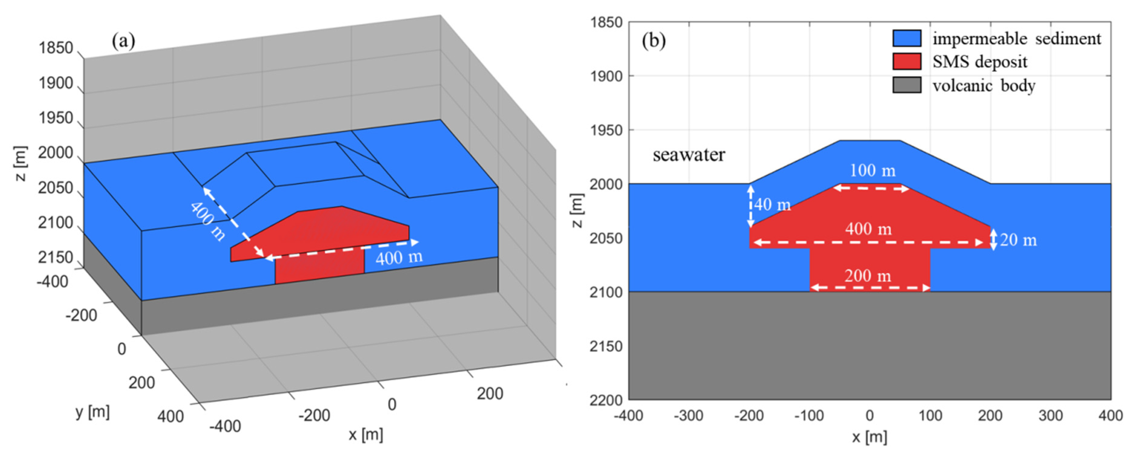
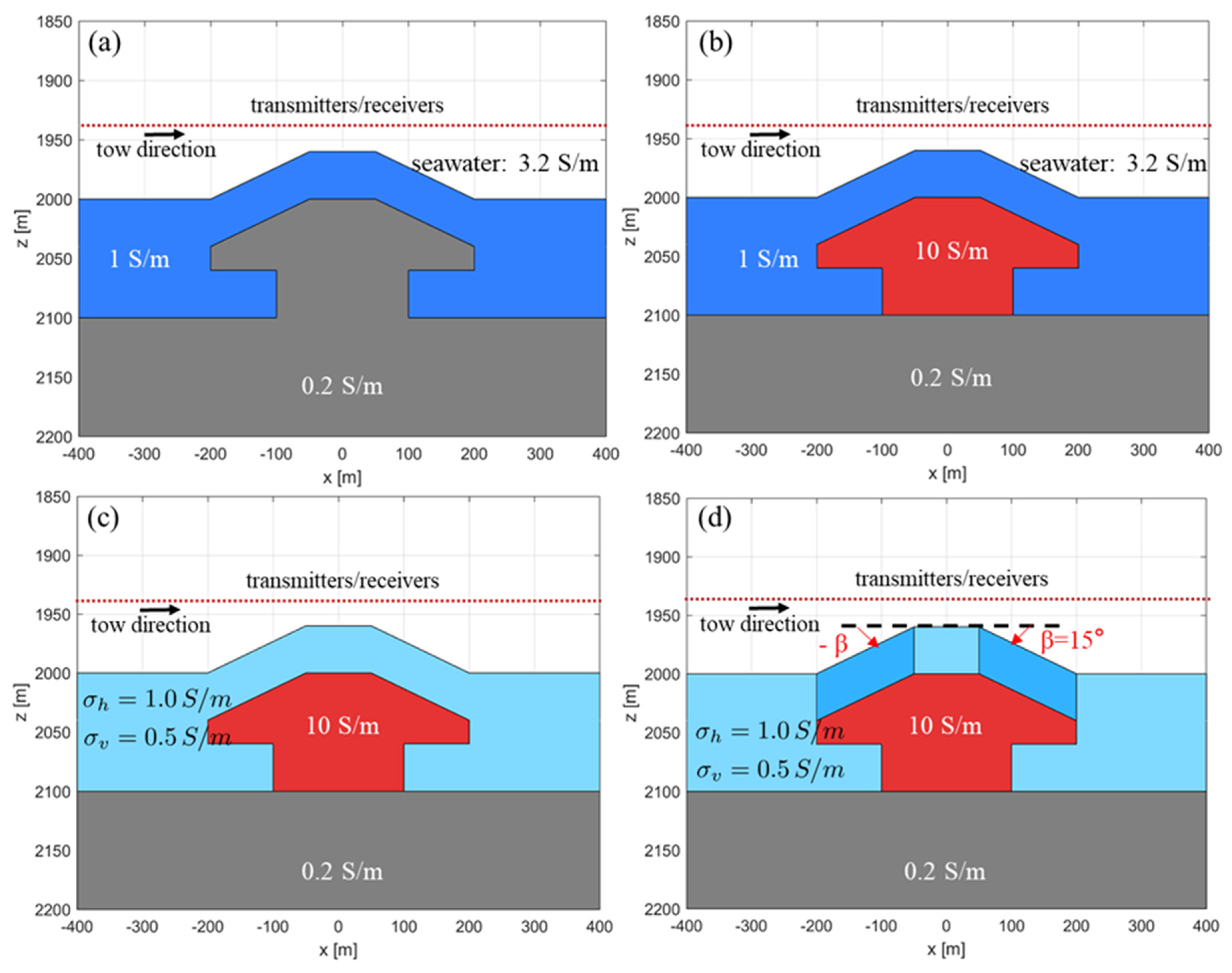
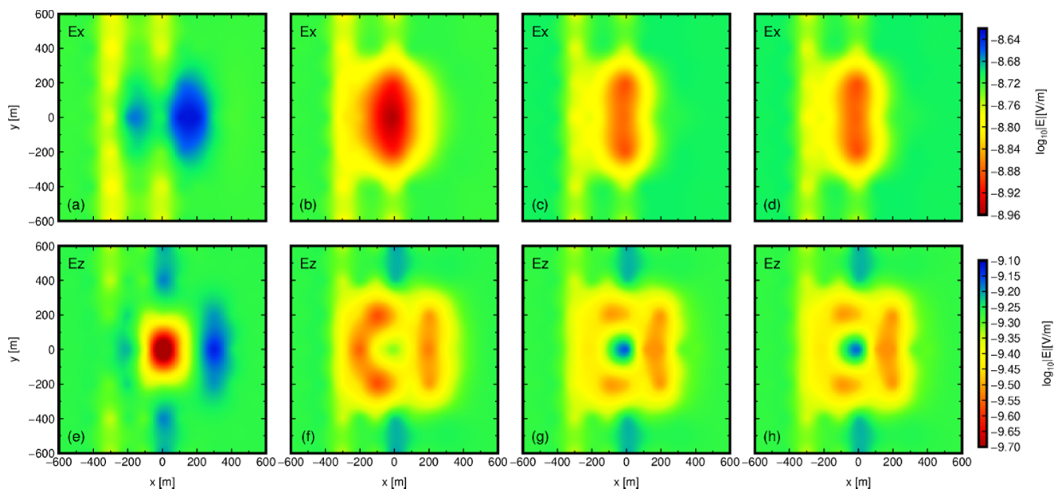
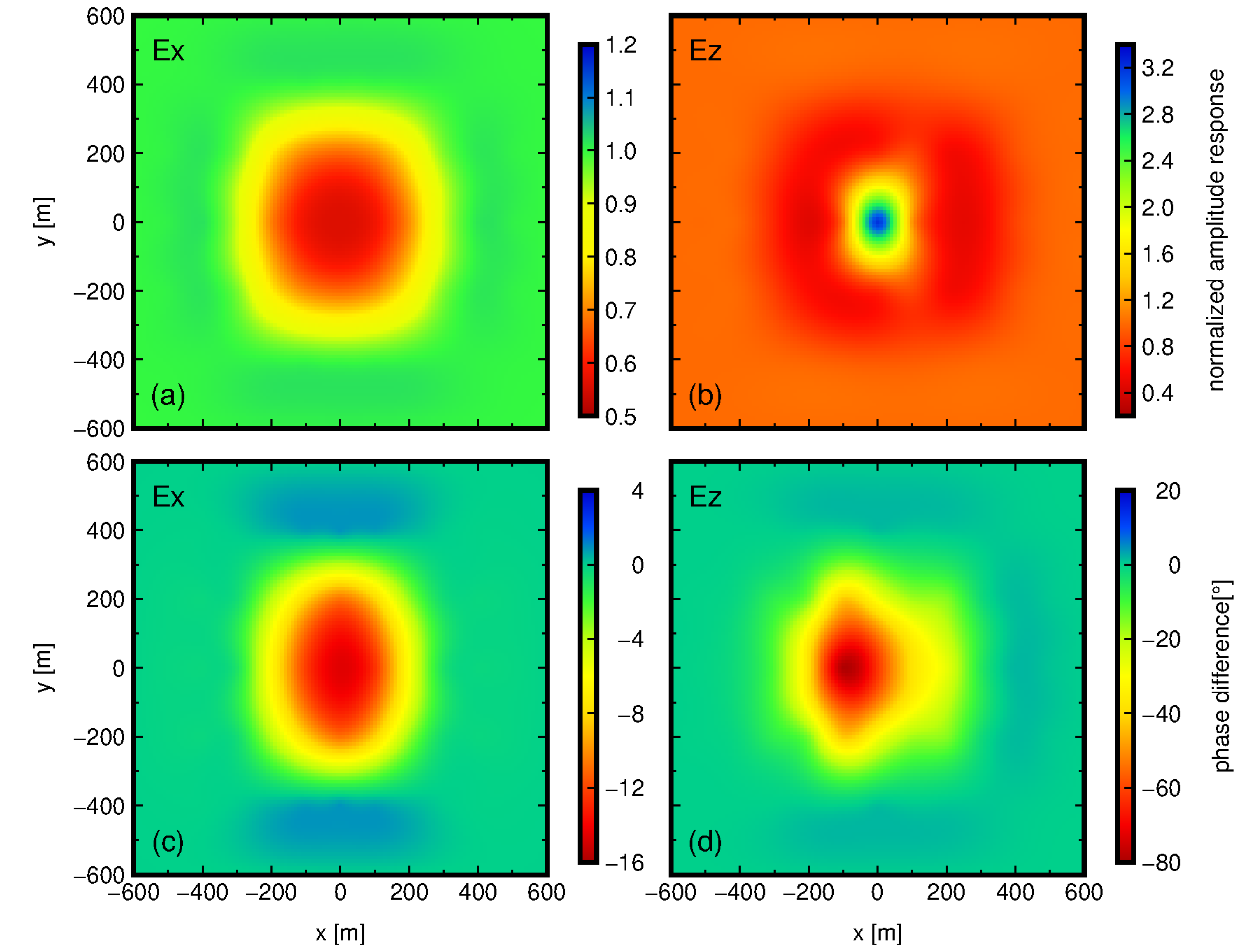
3.2. SMS Model Studies

In this section, we consider a saddle-shaped model to simulate a simplified deep-seated SMS deposit hosted within a continental backarc basin [22], as displayed in Figure 5. A conductive reservoir is introduced to represent buried SMS accumulations. A sedimentary cover of 40 m thick from the top the SMS deposit to the seafloor is characterized with low-permeability and acts as a cap structure to prevent vertical upward migration of hydrothermal fluids, and the sedimentary sequences were uplifted by the volcanic intrusion that forms the submarine knoll [22]. For synthetic modeling studies, we apply a fixed-offset marine CSEM system to simulate the field response. The x-oriented HED transmitter is towed 60 m above the flat seafloor and its elevation is kept constant along the surveying lines. The receiver recording electric fields is located laterally behind the transmitter with an offset of 300 m along the surveying lines.
To investigate the field response of the buried SMS deposit and effects of electrical anisotropy, we simulate the response of the applied CSEM system for four different conductivity models shown in Figure 6. The first model, termed as model 1 in Figure 6a, represents a submarine volcanic knoll without an associated SMS deposit, while the second model (model 2 in Figure 6b) introduces an SMS deposit filling up the knoll. Petrophysical study has revealed that the conductivities of SMS deposits generally vary from 1 to 10 S/m, which are much higher than that of the surrounding volcanic rock [9]. Therefore, we assume that the volcanic body is relatively resistive and has a conductivity of 0.2 S/m, while the conductivity of the SMS deposit is 10 S/m. The sedimentary cover in both models has an isotropic conductivity of 1 S/m [45]. In comparison, the third model (model 3 in Figure 6c) assumes that the sedimentary cover is characterized by weak VTI due to layering or interbedded thin sequences [24]. By contrast, the fourth model (model 4 in Figure 6d) assume that the sedimentary sequence at the flanks of the knoll is characterized by TTI due to the uplifting caused by volcanic intrusions. The sedimentary cover has a horizontal conductivity of 1 S/m and a vertical conductivity of 0.5 S/m, while the flanks in model 4 have an additional dip angle of ±15°.
Figure 7 and Figure 8 demonstrate the amplitude and phase of computed inline (Ex) and vertical (Ez) electric field components for four investigated conductivity models (model 1 to 4) at 2 Hz, respectively. The amplitude distributions displayed in the first column of Figure 7 illustrate obvious filed perturbations due to the presence of the volcanic structure. The second column of Figure 7 shows the amplitude variations caused by the conductive SMS deposit compared to the response of model 1. The third and fourth columns of Figure 7 display additional field perturbations due to electrical anisotropy. To highlight the influence of the SMS deposit, Figure 9 shows the normalized amplitude response (NAR) and phase difference between the model 1 and model 2, and significant amplitude and phase differences are observed within regions of the conductive reservoir. Although the absolute amplitude of Ez component is much smaller than that of Ex (Figure 7), there is nearly a factor of three perturbations in Ez amplitudes (Figure 9b) and 80° variations in Ez phases (Figure 9d), while there is merely a maximum of 50% difference in Ex amplitudes (Figure 9a) and 20° variations in Ex phases (Figure 9c). The significant differences in the NAR of Ex and Ez components imply that the vertical electric field is more sensitive to the perturbations of the conductivity model and is more informative than the inline electric field for laterally heterogeneous structures.
Figure 10 shows the NAR of model 3 with respect to models 1 and 2. The NAR with respect to model 1 (the top panel) represents a combined effect of the conductive SMS deposit and the VTI sedimentary layer. Compared to Figure 8, it is obvious that the presence of the VTI overburden layer affects both electric field amplitudes, but to a different extent. The amplitude differences in the inline field (Ex) reduce about by half compared to that of the isotropic model, making the buried SMS deposit difficult to detect with conventional CSEM survey that utilizes ocean bottom receivers that only record the inline fields. The bottom panel of Figure 10 illustrates the NAR with respect to model 2 that highlights the effects of the electrical anisotropy alone. An apparent increase in both field amplitudes is present within the regions of the conductive reservoir, which implies that the presence of electrical anisotropy in sedimentary formations could mask the responses of the conductive reservoir to some extent, and may lead to underestimation of the SMS anomalies if the anisotropy of the overburden layer is neglected. Figure 11 demonstrates the corresponding phase difference of model 3 with respect to models 1 and 2. The presence of electrical anisotropy has an adverse effect on the Ex and Ez fields, where the phase of Ex (Figure 11c) increases slightly while the phase of Ez (Figure 11d) has a moderate drop.
To evaluate the effects of the TTI anisotropy presented in the flanks of the saddle structure, Figure 12 displays the NAR and phase difference of model 4 with respect to model 3. In contrast to the VTI case, the presence of TTI in both flanks of the saddle structure has a complex influence on the amplitudes within the regions of the conductive reservoir. Although the dip angle of the flanks is quite small (±15°), the maximum amplitude and phase differences in the Ez response between VTI and TTI case reaches nearly 10% (Figure 12b) and 4° (Figure 12d), respectively. This suggests that it could result in an erroneous estimation of the SMS anomalies if the electrical anisotropy is not sufficiently considered.

4. Summary and Conclusions

SMS deposits that have been disconnected to active hydrothermal vents are believed to host a large amount of minerals for prospective mining. Usually, these inactive SMS deposits are likely to be masked by sediments and difficult to be identified. We have developed a finite element modeling approach for marine CSEM surveys for the exploration of SMS deposits. Through numerical simulations, we have confirmed that a fixed-offset marine CSEM method is capable of detecting conductive SMS deposits buried in the shallow regions of the seafloor, as demonstrated by previous studies [4,5,11]. Besides, the results of numerical modeling suggest that the vertical electric fields are more sensitive to small-scale conductivity anomalies than inline electric fields, and contain more information about seafloor conductivity structures. However, they are more susceptible to the distortions caused by the presence of electrical anisotropy in geologic formations, which may bias the data interpretation if the anisotropy is neglected or insufficiently considered.
The 3-D modeling studies illustrate the data acquired by a fixed-offset marine CSEM system are significantly affected by the electrical anisotropy. When the overburden layer is characterized by VTI, the vertical electric field amplitudes have a pronounced increase compared to the isotropic overburden case, and the distortions caused by the anisotropy could mask the CSEM response from the SMS deposits. In these circumstances, the neglect of anisotropic effects would lead to underestimation of the total amount of available SMS deposits based on biased interpretation. In contrast, when the overburden layer is partly characterized by TTI, the vertical electric field amplitudes have a slight increase compared to the VTI overburden case. This implies that insufficient consideration of electrical anisotropy might introduce additional uncertainty in the data interpretation.
Due to the small-scale nature, the SMS deposits masked by sediments are usually difficult to detect. Although our forward modeling studies demonstrate the effectiveness of the fixed-offset marine CSEM method used for SMS exploration, distortions caused by factors such as the bathymetry and electrical anisotropy in practical scenarios may hamper accurate interpretation. Hence, sufficient consideration of electrical anisotropy along with bathymetry are desirable for reliable interpretation of marine CSEM data, thus lending confidence to the estimation of the total amount of available SMS deposits for prospective resource mining.

Author Contributions

Conceptualization, R.P. and X.H.; methodology, R.P. and B.H.; software, R.P.; investigation, R.P. and B.H.; formal analysis, R.P. and B.H.; supervision, X.H.; project administration, X.H.; funding acquisition, Ronghua Peng, B.H., and X.H. All authors have read and agreed to the published version of the manuscript.

Funding

This research was funded by the National Natural Science Foundation of China, grant number 41704133 and 41604063, and Hubei subsurface multi-scale imaging key laboratory, grant number SMIL-2018-03.

Conflicts of Interest

The authors declare no conflict of interest.

References

  1. Hoagland, P.; Beaulieu, S.; Tivey, M.A.; Eggert, R.G.; German, C.; Glowka, L.; Jian, L. Deep-sea mining of seafloor massive sulfides. Mar. Policy 2010, 34, 728–732. [Google Scholar] [CrossRef]
  2. Hölz, S.; Jegen, M. How to Find Buried and Inactive Seafloor Massive Sulfides Using Transient EM-A Case Study from the Palinuro Seamount. In Proceedings of the EAGE/DGG Workshop on Deep Mineral Exploration, Münster, Germany, 18 March 2016. [Google Scholar]
  3. Hölz, S.; Haroon, A.; Jegen, M.; Safipour, R.; Swidinsky, A. Exploration of Seafloor Massive Sulfide Deposits with the Novel EM Induction System MARTEMIS. In Proceedings of the 27. Schmucker-Weidelt Kolloquium für Elektromagnetische Tiefenforschung, Breklum, Germany, 25–29 September 2017. [Google Scholar]
  4. Haroon, A.; Hölz, S.; Gehrmann, R.A.S.; Attias, E.; Jegen, M.; Minshull, T.A.; Murton, B.J. Marine dipole–dipole controlled source electromagnetic and coincident-loop transient electromagnetic experiments to detect seafloor massive sulphides: Effects of three-dimensional bathymetry. Geophys. J. Int. 2018, 215, 2156–2171. [Google Scholar] [CrossRef]
  5. Gehrmann, R.A.S.; North, L.J.; Graber, S.; Szitkar, F.; Petersen, S.; Minshull, T.A.; Murton, B.J. Marine Mineral Exploration with Controlled Source Electromagnetics at the TAG Hydrothermal Field, 26° N Mid-Atlantic Ridge. Geophys. Res. Lett. 2019, 46, 5808–5816. [Google Scholar] [CrossRef] [Green Version]
  6. Hannington, M.; Jamieson, J.; Monecke, T.; Petersen, S.; Beaulieu, S. The abundance of seafloor massive sulfide deposits. Geology 2011, 39, 1155–1158. [Google Scholar] [CrossRef]
  7. Crowhurst, P.; Lowe, J. Exploration and resource drilling of seafloor massive sulfide (SMS) deposits in the Bismarck Sea, Papua New Guinea. In Proceedings of the OCEANS’11 MTS/IEEE KONA, Waikoloa, HI, USA, 19–22 September 2011; pp. 1–6. [Google Scholar]
  8. Schwalenberg, K.; Müller, H.; Engels, M. Seafloor Massive Sulfide Exploration—A New Field of Activity for Marine Electromagnetics. In Proceedings of the EAGE/DGG Workshop on Deep Mineral Exploration, Münster, Germany, 18 March 2016. [Google Scholar]
  9. Spagnoli, G.; Hannington, M.; Bairlein, K.; Hördt, A.; Jegen, M.; Petersen, S.; Laurila, T. Electrical properties of seafloor massive sulfides. Geo-Mar. Lett. 2016, 36, 235–245. [Google Scholar] [CrossRef]
  10. Spagnoli, G.; Weymer, B.A.; Jegen, M.; Spangenberg, E.; Petersen, S. P-wave velocity measurements for preliminary assessments of the mineralization in seafloor massive sulfide mini-cores during drilling operations. Engineering Geology 2017, 226, 316–325. [Google Scholar] [CrossRef] [Green Version]
  11. Müller, H.; Schwalenberg, K.; Reeck, K.; Barckhausen, U.; Schwarz-Schampera, U.; Hilgenfeldt, C.; von Dobeneck, T. Mapping seafloor massive sulfides with the Golden Eye frequency-domain EM profiler. First Break 2018, 36, 61–67. [Google Scholar]
  12. Cheesman, S.; Edwards, R.; Chavez, A. On the theory of sea floor conductivity mapping using transient EM systems. Geophysics 1987, 52. [Google Scholar] [CrossRef] [Green Version]
  13. Weitemeyer, K.A.; Constable, S.C.; Key, K.W.; Behrens, J.P. First results from a marine controlled-source electromagnetic survey to detect gas hydrates offshore Oregon. Geophys. Res. Lett. 2006, 33. [Google Scholar] [CrossRef] [Green Version]
  14. Constable, S. Ten years of marine CSEM for hydrocarbon exploration. Geophysics 2010, 75, A67–A75. [Google Scholar] [CrossRef] [Green Version]
  15. Schwalenberg, K.; Rippe, D.; Koch, S.; Scholl, C. Marine-controlled source electromagnetic study of methane seeps and gas hydrates at Opouawe Bank, Hikurangi Margin, New Zealand. J. Geophys. Res. Solid Earth 2017, 122, 3334–3350. [Google Scholar] [CrossRef] [Green Version]
  16. Cairns, G.W.; Evans, R.L.; Edwards, R.N. A time domain electromagnetic survey of the TAG Hydrothermal Mound. Geophys. Res. Lett. 1996, 23, 3455–3458. [Google Scholar] [CrossRef]
  17. Kowalczyk, P. Geophysical prelude to first exploitation of submarine massive sulphides. First Break 2008, 26, 99–106. [Google Scholar]
  18. Müller, H.; Schwalenberg, K. Electromagnetic imaging of seafloor massive sulfide deposits at the Central Indian Ridge. In Proceedings of the EGU General Assembly, Vienna, Austria, 17–22 April 2016. [Google Scholar]
  19. Constable, S.; Kowalczyk, P.; Bloomer, S. Measuring marine self-potential using an autonomous underwater vehicle. Geophys. J. Int. 2018, 215, 49–60. [Google Scholar] [CrossRef]
  20. Ishizu, K.; Goto, T.; Ohta, Y.; Kasaya, T.; Iwamoto, H.; Vachiratienchai, C.; Siripunvaraporn, W.; Tsuji, T.; Kumagai, H.; Koike, K. Internal Structure of a Seafloor Massive Sulfide Deposit by Electrical Resistivity Tomography, Okinawa Trough. Geophys. Res. Lett. 2019, 46, 11025–11034. [Google Scholar] [CrossRef]
  21. Masaki, Y.; Kinoshita, M.; Inagaki, F.; Nakagawa, S.; Takai, K. Possible kilometer-scale hydrothermal circulation within the Iheya-North field, mid-Okinawa Trough, as inferred from heat flow data. JAMSTEC Rep. Res. Dev. 2011, 12, 1–12. [Google Scholar] [CrossRef] [Green Version]
  22. Tsuji, T.; Takai, K.; Oiwane, H.; Nakamura, Y.; Masaki, Y.; Kumagai, H.; Kinoshita, M.; Yamamoto, F.; Okano, T.; Kuramoto, S.I. Hydrothermal fluid flow system around the Iheya North Knoll in the mid-Okinawa trough based on seismic reflection data. J. Volcanol. Geotherm. Res. 2012, 213–214, 41–50. [Google Scholar] [CrossRef] [Green Version]
  23. Mendelson, K.S.; Cohen, M.H. The effect of grain anisotropy on the electrical properties of sedimentary rocks. Geophysics 1982, 47, 257–263. [Google Scholar] [CrossRef]
  24. Anderson, B.; Bryant, I.; Luling, M.; Spies, B.; Helbig, K. Oilfield anisotropy: Its origins and electrical characteristics. Oilfield Rev. 1994, 6, 48–56. [Google Scholar]
  25. Klein, J.D.; Martin, P. The petrophysics of electrically anisotropic reservoirs. Log Anal. 1997, 38, 25–36. [Google Scholar]
  26. Yu, L.; Edwards, R. The detection of lateral anisotropy of the ocean floor by electromagnetic methods. Geophys. J. Int. 1992, 108, 433–441. [Google Scholar] [CrossRef] [Green Version]
  27. Newman, G.A.; Commer, M.; Carazzone, J.J. Imaging CSEM data in the presence of electrical anisotropy. Geophysics 2010, 75, F51–F61. [Google Scholar] [CrossRef]
  28. Li, Y.; Dai, S. Finite element modelling of marine controlled-source electromagnetic responses in two-dimensional dipping anisotropic conductivity structures. Geophys. J. Int. 2011, 185, 622–636. [Google Scholar] [CrossRef] [Green Version]
  29. Tompkins, M.J. The role of vertical anisotropy in interpreting marine controlled-source electromagnetic data. In Proceedings of the 2005 SEG Annual Meeting, Houston, TX, USA, 6–11 November 2005. [Google Scholar]
  30. Jaysaval, P.; Shantsev, D.V.; de Ryhove, S.d.l.K.; Bratteland, T. Fully anisotropic 3-D EM modelling on a Lebedev grid with a multigrid pre-conditioner. Geophys. J. Int. 2016, 207, 1554–1572. [Google Scholar] [CrossRef] [Green Version]
  31. Peng, R.; Hu, X.; Chen, B.; Li, J. 3-D Marine controlled-source electromagnetic modeling in electrically anisotropic formations using scattered scalar–vector potentials. IEEE Geosci. Remote Sens. Lett. 2018, 15, 1500–1504. [Google Scholar] [CrossRef]
  32. Davydycheva, S.; Frenkel, M.A. The impact of 3D tilted resistivity anisotropy on marine CSEM measurements. Lead. Edge 2013, 32, 1374–1381. [Google Scholar] [CrossRef]
  33. Gehrmann, R.; Haroon, A.; Morton, M.; Djanni Minshull, T. Seafloor massive sulphide exploration using deep-towed controlled source electromagnetics: Navigational uncertainties. Geophys. J. Int. 2020, 220, 1215–1227. [Google Scholar] [CrossRef]
  34. Constable, S.; Kannberg, P.K.; Weitemeyer, K. Vulcan: A deep-towed CSEM receiver. Geochem. Geophys. Geosyst. 2016. [CrossRef] [Green Version]
  35. Attias, E.; Weitemeyer, K.; Hölz, S.; Naif, S.; Minshull, T.A.; Best, A.I.; Haroon, A.; Jegen-Kulcsar, M.; Berndt, C. High-resolution resistivity imaging of marine gas hydrate structures by combined inversion of CSEM towed and ocean-bottom receiver data. Geophys. J. Int. 2018, 214, 1701–1714. [Google Scholar] [CrossRef]
  36. Pek, J.; Santos, F.A.M. Magnetotelluric inversion for anisotropic conductivities in layered media. Phys. Earth Planet. Inter. 2006, 158, 139–158. [Google Scholar] [CrossRef]
  37. Ward, S.; Hohmann, G. Electromagnetic Methods in Applied Geophysics Vol. I. Investigations in Geophysics; SEG: Tulsa, OK, USA, 1988. [Google Scholar]
  38. Lynch, D.R.; Paulsen, K.D. Origin of vector parasites in numerical Maxwell solutions. IEEE Trans. Microw. Theory Tech. 1991, 39, 383–394. [Google Scholar] [CrossRef]
  39. Monk, P. Finite Element Methods for Maxwell’s Equations; Oxford University Press: Oxford, UK, 2003. [Google Scholar]
  40. Jin, J. The Finite Element Method in Electromagnetics, 3rd ed.; John Wiley & Sons: Hoboken, NJ, USA, 2014. [Google Scholar]
  41. Ansari, S.; Farquharson, C.G. 3D finite-element forward modeling of electromagnetic data using vector and scalar potentials and unstructured grids. Geophysics 2014, 79. [Google Scholar] [CrossRef]
  42. Si, H. TetGen, a Delaunay-Based Quality Tetrahedral Mesh Generator. ACM Trans. Math. Softw. (TOMS) 2015, 41, 11. [Google Scholar] [CrossRef]
  43. Saad, Y. Iterative Methods for Sparse Linear Systems; Siam: University City, PA, USA, 2003. [Google Scholar]
  44. Hunziker, J.; Thorbecke, J.; Slob, E. The electromagnetic response in a layered vertical transverse isotropic medium: A new look at an old problem. Geophysics 2014, 80, F1–F18. [Google Scholar] [CrossRef] [Green Version]
  45. Boyce, R.E. Electrical resistivity of modern marine sediments from the Bering Sea. J. Geophys. Res. 1968, 73, 4759–4766. [Google Scholar] [CrossRef]
Figure 1. Schematic representation of the fixed-offset controlled-source electromagnetic method (CSEM) system [34] applied in exploration of seafloor massive sulfide (SMS) deposits. A horizontal electric dipole source is towed close to the seafloor, and the electromagnetic fields are recorded by receivers towed behind the transmitter.
Minerals 10 00457 g001
Figure 2. Degrees of freedom associated with a tetrahedral element. The vector potential is constructed by linear interpolation of the tangential component on each edge, while the scalar potential is constructed by linear interpolation of the scalar value on each node.
Minerals 10 00457 g002
Figure 3. A deep-water layered anisotropic model with a conductive SMS layer covered by seafloor sediments.
Minerals 10 00457 g003
Figure 4. Comparison between the finite element (FE) (symbols) and quasi-analytic (lines) solutions for the deep-water layered anisotropic model. Amplitude (a) and phase (b) of the Ex and Ez components denoted by circles and squares, respectively. Corresponding relative amplitude errors (c) and phase differences (d) between the FE and quasi-analytic solutions.
Minerals 10 00457 g004
Figure 5. Illustration of a saddle model used for 3-D forward modeling studies, water depth is 2000 m. (a) 3-D view of the saddle structure. (b) Schematic of the model dimensions in the x-z plane at y = 0 m.
Minerals 10 00457 g005
Figure 6. 2-D cross-section (x-z plane) through the submarine knoll center of the four 3-D conductivity models investigated in forward modeling studies. During the survey, the CSEM system is towed from left to right along the surveying line with the transmitter on the right. The four considered conductivity models are illustrated in (ad).
Minerals 10 00457 g006
Figure 7. Amplitude of the inline electric fields at a frequency of 2 Hz for four considered models (model 1 to 4) are displayed in (ad), and amplitude of the vertical electric fields in (eh). Note that the fields are plotted at the midpoint of the transmitter and receiver.
Minerals 10 00457 g007
Figure 8. Phase of the inline electric fields at a frequency of 2 Hz for four considered models (model 1 to 4) are displayed in (ad), and phase of the vertical electrical fields in (eh). Note that the fields are plotted at the midpoint of the transmitter and receiver.
Minerals 10 00457 g008
Figure 9. The normalized amplitude response of model 2 with respect to model 1 is calculated for Ex (a) and Ez (b), and corresponding phase difference for Ex (c) and Ez (d).
Minerals 10 00457 g009
Figure 10. The normalized amplitude response of model 3 with respect to model 1 is calculated for Ex (a) and Ez (b), and that of model 3 with respect to model 2 for Ex (c) and Ez (d).
Minerals 10 00457 g010
Figure 11. The phase difference of model 3 with respect to model 1 is calculated for Ex (a) and Ez (b); and that of model 3 with respect to model 2 for Ex (c) and Ez (d).
Minerals 10 00457 g011
Figure 12. The normalized amplitude response of model 4 with respect to model 3 is calculated for Ex (a) and Ez (b), and corresponding phase difference for Ex (c) and Ez (d) to quantify the effects of dipping electrical anisotropy.
Minerals 10 00457 g012

