In this section, a comparison between the BEM and the RANSE solvers is presented in a case of a steady foil beneath the free surface (
Section 4.1). Then, the mixed frequency–time domain method presented in
Section 2 is exploited to obtain the kinematics of the ship and wing in waves and study the performance of the flapping thruster using the BEM solver (
Section 4.2). Results concerning the flapping foil at great submergence (without free-surface effects) are presented in
Section 4.3, and close to the free surface in
Section 4.4, as obtained by using the BEM and RANSE solvers. Finally, in
Section 4.5 systematic investigation of free-surface, viscosity, and incident-wave effects is presented and discussed including convergence study of both solvers.
4.2. Foil Motion and BEM Calculations in Waves
Next, unsteady numerical calculations are presented in
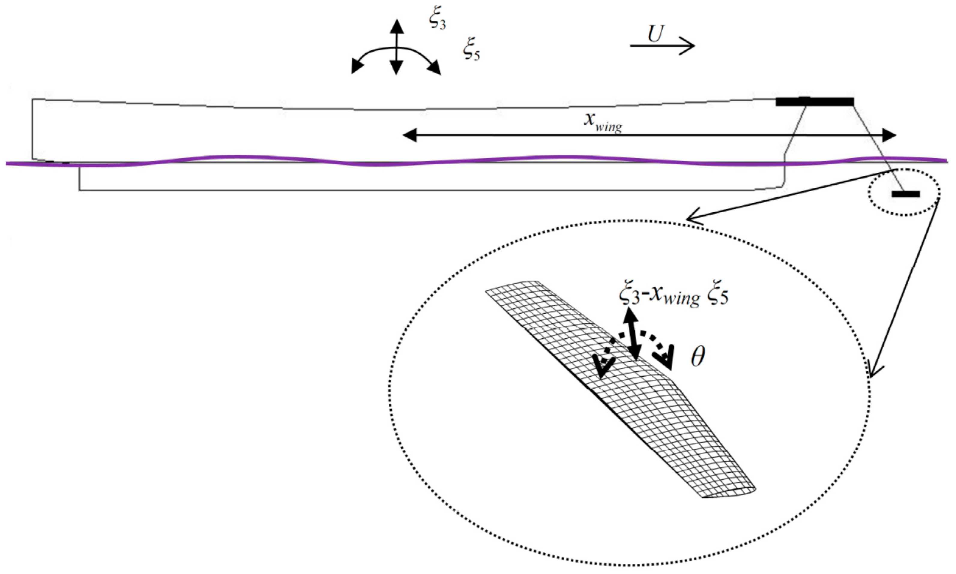
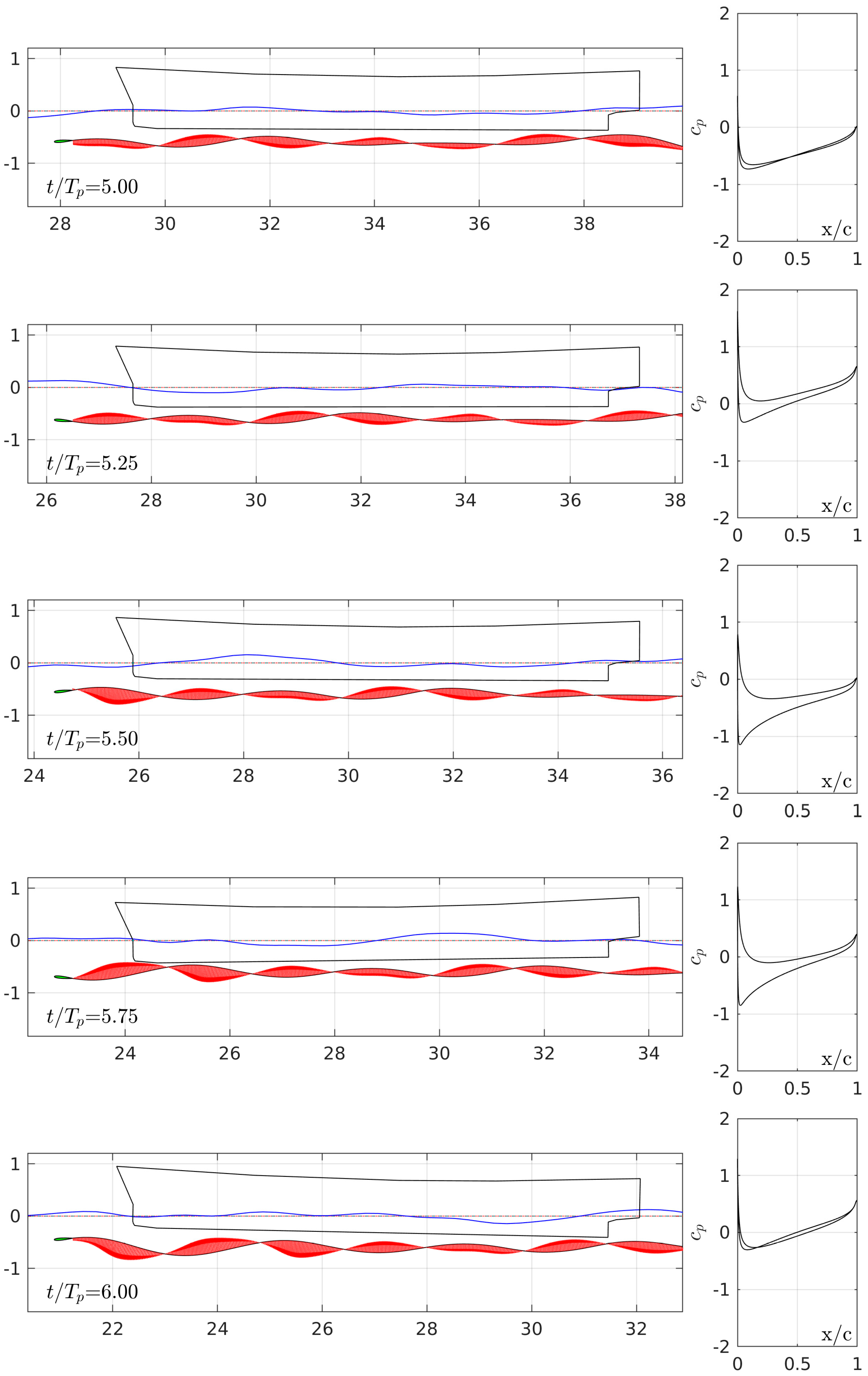
Figure 9, considering the performance of the flapping thruster in the bow of the ship subjected to vertical oscillations due to ship responses in head waves and at the same time performing self-pitching oscillations about its pivot axis at
with controllable amplitude based on its vertical motion, as described in previous
Section 2 and
Section 3.1. The flapping foil is located at the same mean submergence
, advancing with the same as before velocity
, in irregular waves (
and Strouhal number
, where
is the frequency of encounter that corresponds to the peak period of the spectrum; see
Section 2.
Calculations have been done by using pitch control parameter
. In particular, in
Figure 9, the ship travelling in irregular waves is shown at five instants within a time interval corresponding to one modal period. The foil is located in front of the bow of the ship, at distance x
wing/L = 0.6 with respect to the midship section of the ship. In the same figure, the foil wake is plotted, with the calculated dipole intensity (potential jump) on the vortex sheet, which is illustrated by using arrows normal to the wake curve with length proportional to the local dipole strength. The latter result is associated with the memory effect of the generated lifting flow around the flapping foil operating in random incident waves.
Moreover, in the right subplots of
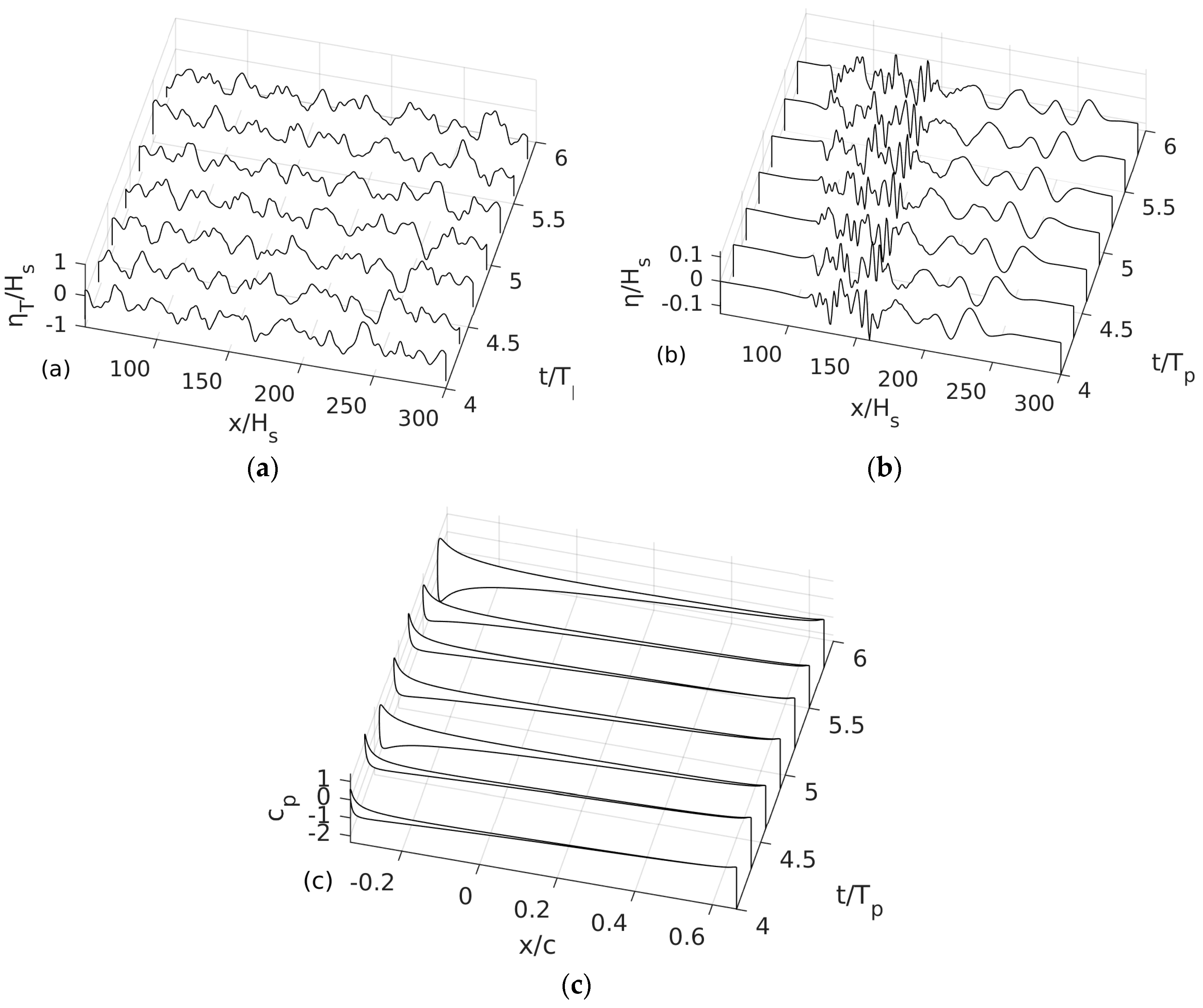
Figure 9, the instantaneous distribution of the pressure coefficient on the foil, at the same time instants, as calculated by the present method. From the calculated pressure distributions, lift and thrust components are obtained at each time step by integration. In order to illustrate the relative magnitude of the incident and disturbance flow generated by the flapping motion of the foil in waves, for the same as before wave conditions and hydrofoil data, the calculated free-surface elevation normalized with respect to the significant wave height plotted in
Figure 10 over the horizontal domain, at some instances during two modal periods.
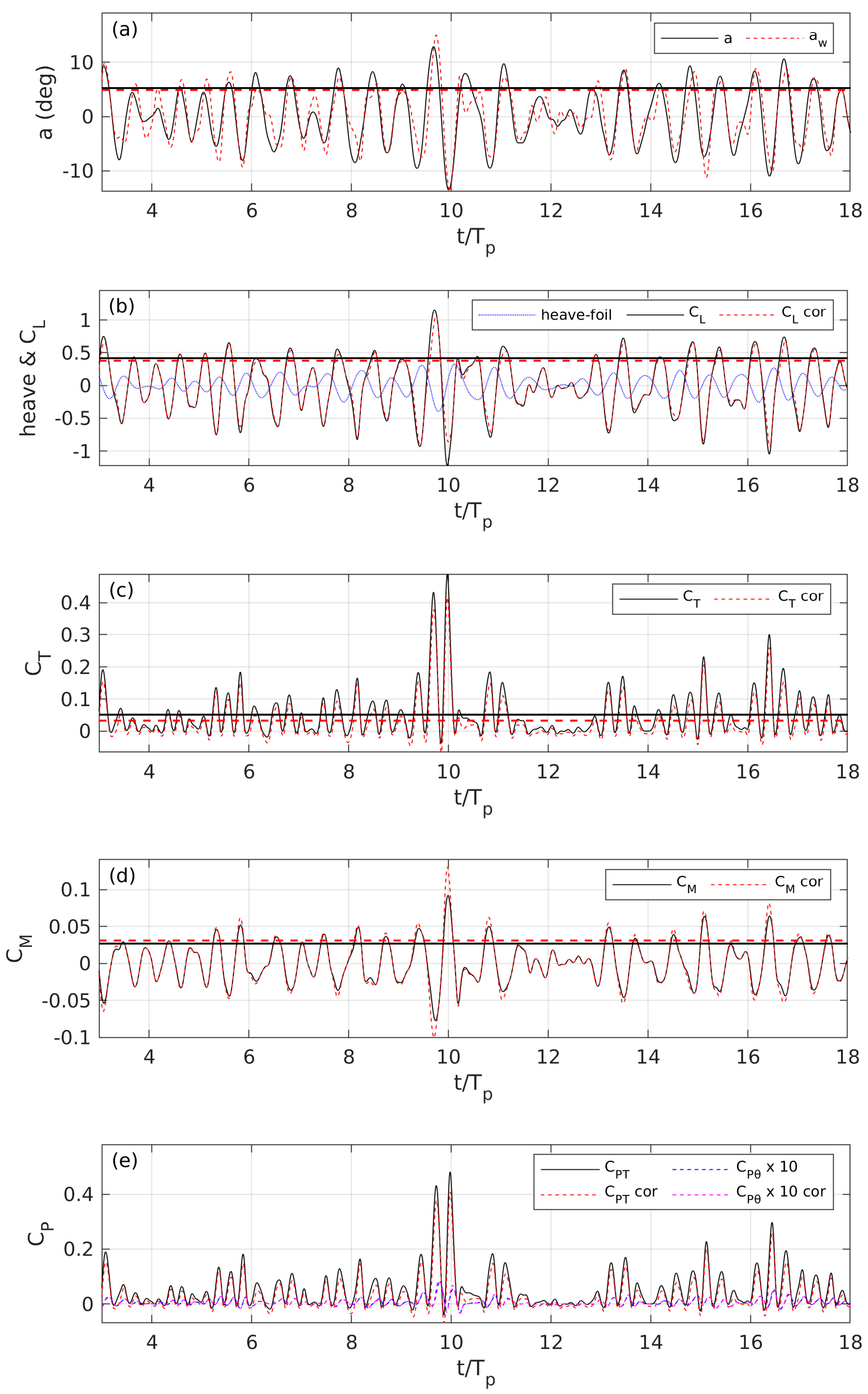
Furthermore, we present in
Figure 11 the time series of several calculated quantities concerning thrust production by the examined system, as calculated by the present BEM for a time interval from 3 to 18 peak periods. The dynamic system is integrated starting from rest, and the transient effects have been died out in the first three periods. The responses of the examined ship and flapping foil system in waves are calculated by both the present BEM without (solid line) and with viscous corrections.
In particular, in
Figure 11a, the time history of the angle of attack is presented excluding
and including
the effects of the incident wave field. The angle is calculated using Equation (5) and the effects of the free surface, the disturbance of the foil and the wake are approximately excluded from the calculation. The effect of the wave is either to increase or decrease the temporal value of the angle of attack by a small amount, resulting in a maximum value of
instead of
(at
), and slightly reduce the corresponding rms value from
to
. In general, the angle of attack is an indicator of the importance of viscous effects, which remain at moderate levels, rendering cost-effective potential methods capable to provide accurate predictions for the design of flapping foil thrusters as will be illustrated in the sequel through comparison against RANSE calculations in
Section 4.3,
Section 4.4 and
Section 4.5.
In
Figure 11b, we present the time history of foil’s heaving motion, as produced by combined oscillatory heaving and pitching motion of the coupled ship-flapping foil system, together with the generated sectional lift coefficient
. We observe that significant amplitudes of the lift force are produced. Moreover, the phase lag between foil’s motion and lift force is approximately
; Therefore, the generated lift acts as a restoring force, reducing the responses of a ship equipped with flapping hydrofoils. In
Figure 11c, the dynamic evolution of sectional thrust coefficient
is shown, in the same time interval. We observe in this subplot that the thrust oscillations are in the interval
, with an average value of
for the purely potential calculation, which is indicated by a horizontal black solid line and
for the corrected results indicated with a horizontal red dashed line. Although viscous effects cause almost a
decrease in mean value, the corresponding decrease is only
as concerns the peak value. In the examined case, the thrust production compared to the calm water resistance is found to reach levels of the order of 30%, which is considered to be important.
Additionally, the time history of moment required for the active pitching motion of the foil is presented in
Figure 11d in terms of sectional moment coefficient
. As expected, viscous corrections increase the required torque input for the system to operate. Moreover, in
Figure 11e, the power extracted by the examined system from the waves
is compared against the corresponding power that is necessary for the self-pitching motion of the foil
, actually for tuning the instantaneous angle of attack in order to produce positive thrust. We observe that the latter quantity is practically insignificant and that the viscous effects modify slightly the predictions by reducing
and increasing
. In the present section, the wave effects in the performance of the foil have been studied by means of a BEM and the effects of viscosity have been considered using empirical corrections. In the following subsections, the effects of viscosity and the free-surface boundary are also investigated by means of the CFD model and comparison between the BEM and RANSE are presented and discussed. First, in
Section 4.3, the effects of the free-surface are neglected in order to derive calibration factors for the BEM model for viscous corrections. Subsequently, in
Section 4.4, both models are applied and the predictions including the free-surface effects are compared.
4.3. BEM and RANSE Calculations of Flapping Foil in Unbounded Domain—Calibration of Viscous Corrections
In the present subsection, the effects of the wave and the free surface boundary are excluded from the modeling in order to derive estimates of the effects of viscosity for the flapping thruster. BEM and RANS calculations are compared to identify the range of applicability and the limitations of each scheme and to calibrate the correction formula (Equation (22)). To be more specific, in
Figure 12,
Figure 13 and
Figure 14, simulations with both numerical methods are presented for a flapping foil in heaving motion, pitching motion, and angle of attack as in
Figure 11.
In
Figure 12, we present snapshots for three time instances of foil simulation using a cost effective potential method and the high fidelity viscous solver for a time interval of one peak period. In the BEM case, where a simplified wake model is used, the trailing vortex curve modeling the foil’s wake is plotted, including the calculated dipole intensity (potential jump) on the vortex sheet, which is illustrated by using arrows normal to the wake curve with length proportional to the local dipole strength. In the RANSE simulations, the wake is resolved in more detail and the vorticity contours are illustrated with different colors. A reverse Kármán vortex street pattern of moderate intensity and size is generated downstream to the foil as expected from the operation of flapping foils in relatively low Strouhal numbers and moderate angles of attack. Ιn most cases, even with the simplified wake model, the location of maximum vorticity
coincides with the critical points of dipole intensity
μ. The differences in the BEM case are attributed to the linearization of the vortex wake dynamics and could be overcome by using a fully nonlinear wake model [
20,
42]. In the same figure, the pressure distribution is plotted at three time instances
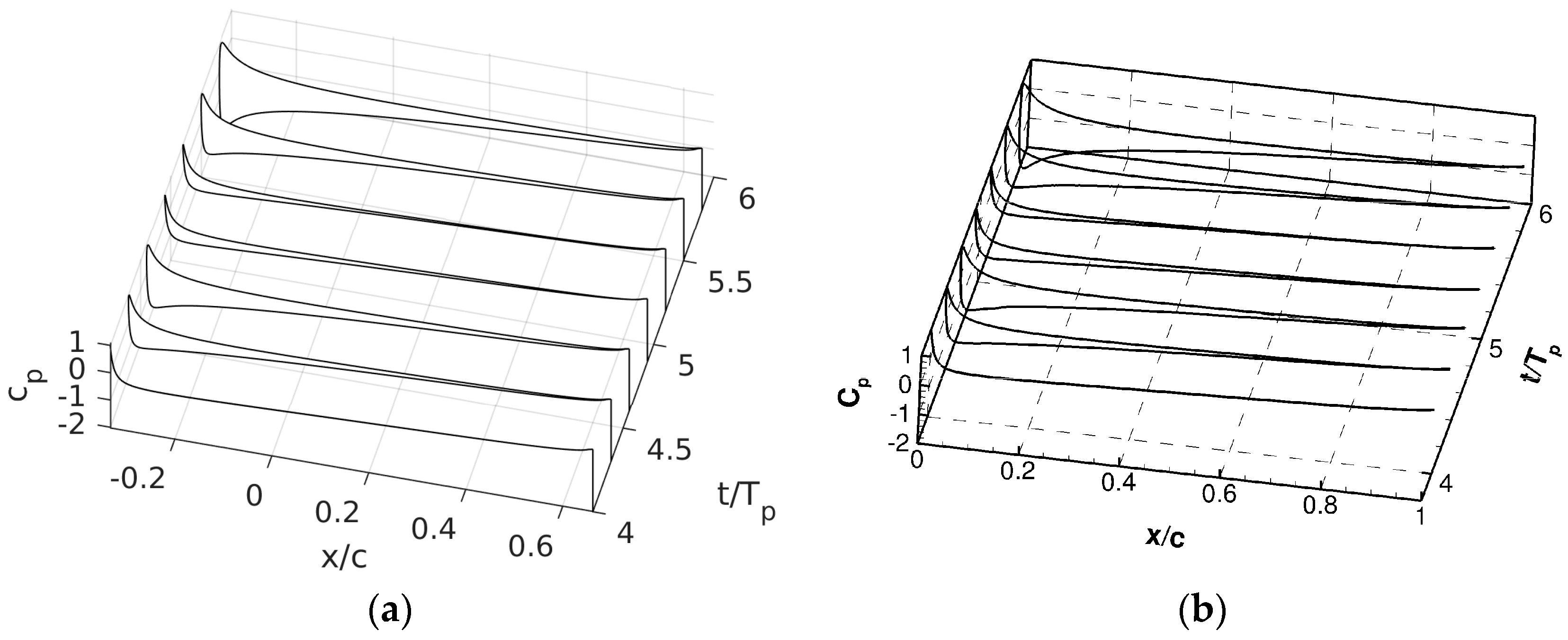
, as calculated by BEM and RANSE. Moreover, in
Figure 13, a more detailed representation of the pressure distribution evolution during for the 5th and 6th period of simulation is illustrated. Very good agreement is observed with insignificant discrepancies at the neighborhoods of the leading and the trailing edges.
In
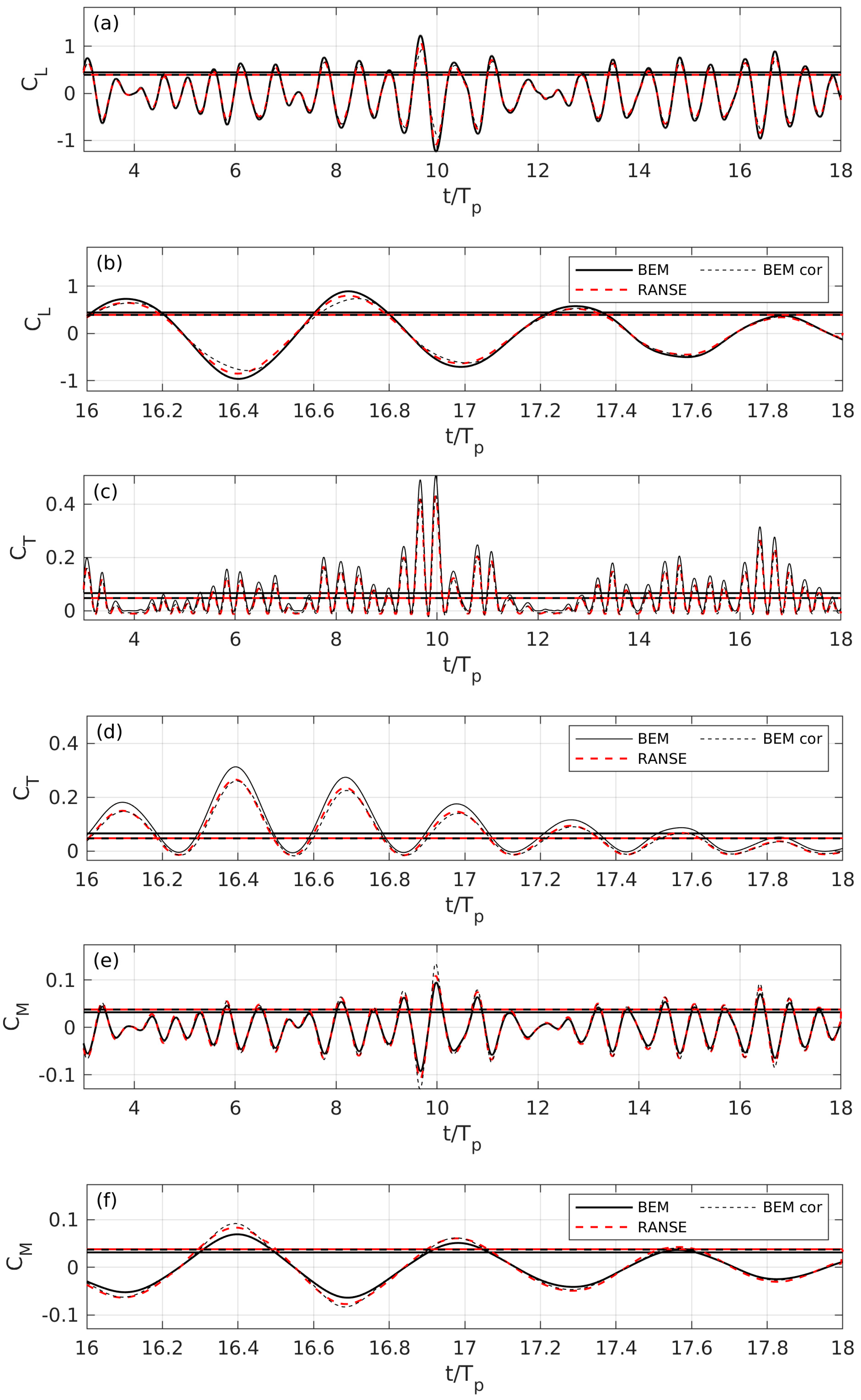
Figure 14, we present the loads of the system in waves in unbounded domain, as calculated by the present BEM including corrections and RANSE. In subplots (a), (c), and (e), the plots of
histories are presented, respectively, whereas in subplots (b), (d), and (f), details during the 16th and 17th period are provided for comparison between the two methods.
The lift oscillations are in the interval , with an rms value of for the BEM calculation and for RANSE. Although viscous effects cause almost a decrease in rms value of lift, the reduction is only of the maximum peak value. The thrust oscillations are in the interval , with a mean value of as obtained from BEM and from RANSE. Although viscous effects cause almost a decrease in mean value of thrust, the reduction is only of the maximum peak value. The moment oscillations are in the interval from BEM reaching the maximum value of 0.094, with mean value of . The corresponding value for RANSE is . Although viscous effects cause almost a increase in rms value of foil self-pitching moment, that increase is only of the maximum peak value. The corrected BEM results with appropriate selection of coefficient provide compatible predictions with CFD model.
4.4. BEM and RANSE Calculation of Flapping Foil Beneath the Free Surface
Following the previous analysis, in this section the effect of the free surface is now taken into account. The flapping foil undergoes the same heaving and pitching motion as before, advancing with the same forward speed
. However, now it is considered completely submerged at a depth
as in
Section 4.2. A comparison between BEM and RANS numerical predictions is presented in terms of foil loading as well as the foil-induced wave system.
In
Figure 15, three snapshots of the flapping foil numerical predictions can be seen. BEM and RANSE simulations are presented during a time interval of one peak period. As in the previous subsection, BEM results concerning the dipole intensity in the vortex wake are shown, while for the CFD predictions vorticity contours are plotted.
Comparing the wake evolution between the two methods, it is clear that there is good qualitative agreement between the two solvers. Indeed, as the instantaneous pressure coefficients suggest (
Figure 15), results are consistent between the two numerical methods. As stated in the previous section, apart from the absence of viscosity in the BEM predictions, the discrepancies between the two methods are due to the linearization of the wake vortex dynamics. When the free surfaces are considered, another source of error between the two methods emerges since the way the free surface is modeled is completely different. For the RANSE simulations the VOF approach is employed and thus the free surface is not explicitly defined. On the other hand, in the BEM approach, the free surface elevation is calculated as an explicit function of horizontal space variable
x, also linearization of free-surface boundary conditions has been applied.
In
Figure 16, the free surface elevation as well as the pressure distribution are plotted seven times between the 4th and the 6th period. It is observed that BEM and RANSE are in very good agreement both for the predicted free surface elevation as well as for the instantaneous pressure coefficient. It is noted that, contrary to the RANSE simulations (where the foil is stationary and the flow comes with
), in the case BEM, the problem is solved in the earth-fixed frame of reference (the foil is travelling with forward speed
). However, the results in
Figure 15 suggest that the predicted surface elevation in the near-foil regime is in very good agreement between the two methods. The same can be concluded by comparing the pressure coefficients presented in
Figure 16c,d, from which it is evident that both solvers predict the very similar results for
.
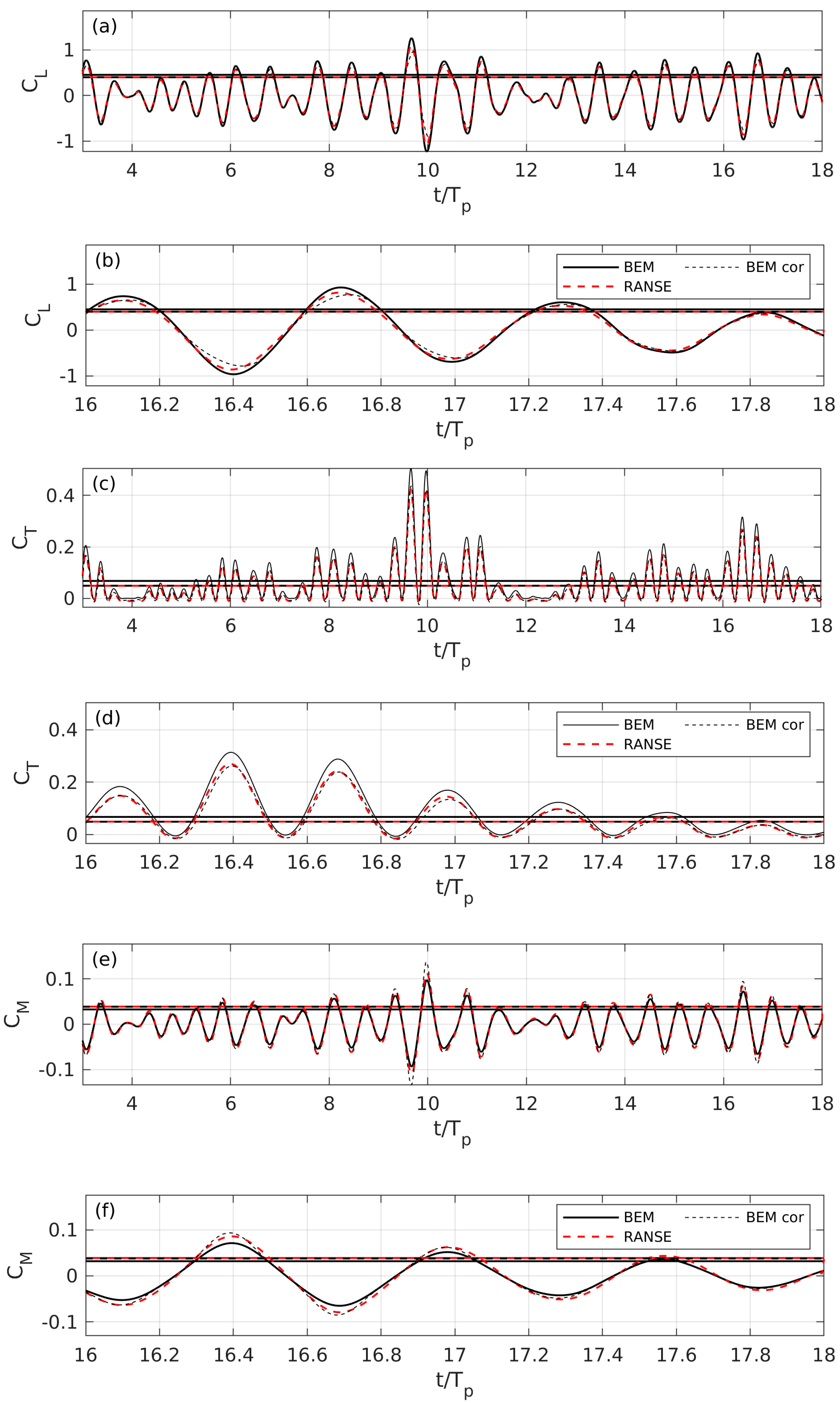
Finally, in
Figure 17, we present the evolution of the forces and moment acting of the flapping foil operating beneath the free surface for the simulation of
Figure 15. Good comparison between the present BEM and RANSE results is obtained. Moreover, calculations with the corrected BEM method are provided in the same figure. The viscous corrections are calibrated using the results of
Section 4.3 for time integrated values (average and RMS). Again, simulation is over 18 peak periods, and the time-integrated quantities (averaged and RMS values calculated excluding the first 3 periods) are presented with horizontal lines. In
Figure 17a,c,e, the time history of force coefficients is presented, whereas in
Figure 17b,d,f, details during the time interval between 16th and 17th period are provided.
The sectional lift coefficient oscillations are found to be in the interval that is slightly wider than the corresponding interval calculated in the previous section in unbounded domain (). The sectional lift coefficient obtained from BEM has an rms value of and from RANSE. The corresponding rms values in unbounded domain were of similar levels; i.e., 0.45 and 0.39. Although viscous effects cause almost an decrease in rms value, the reduction is only of the maximum peak value.
The thrust oscillations are in the interval very similar with the corresponding result in unbounded domain (). Thrust has a mean value of calculated from BEM and from RANSE, respectively. The corresponding mean values in the unbounded domain are quite similar. Although viscous effects cause almost a decrease in mean value, the reduction is only of the maximum peak value.
The self-pitching moment oscillations are in the interval from BEM, reaching a maximum value of 0.097 and rms value , while the prediction from CFD analysis is . The corresponding mean values in unbounded domain were found to be very similar. Although viscous effects cause almost a increase in rms value, the increase is only of the maximum peak value. In the present case, where free-surface effects are considered, the corrected BEM predictions differ only at the third significant digit from the corresponding CFD. Moreover, the empirical corrections reduce the discrepancies at the peaks between BEM and RANSE calculations. Therefore, in the present case of Froude number and mean submergence , free-surface boundary does not affect significantly the calculations, and calibration using only one unbounded domain simulation is sufficient.
4.5. Effects of Waves, Free Surface, Viscosity, and Numerical Convergence
In this section, detailed investigation of viscosity, free-surface, and wave effects in a wide range of mean submergence of the flapping thruster is performed. Moreover, a detailed convergence study of the two numerical schemes is presented. In all cases, a NACA0012 heaving foil is considered in forward motion that corresponds to
simultaneously pitching about a pivot axis located on the chord at distance
from the leading edge, resulting in angle of attack
and kinematics given in
Figure 11.
The calculations in the unbounded domain are labeled as “inf” in
Figure 18, while the calculations of the foil beneath the free surface without incident waves are denoted with “fs” and the calculations in irregular waves corresponding to
and Strouhal number
are denoted with label “wave”. The mean submergence parameter
varies from 1.14 to 18.29 and even in the “wave” calculations the same foil kinematics are used (ignoring the effect of the varying foil submergence to the ship-foil RAO). In all cases, BEM calculation with viscous corrections are also presented. The latter corrections are calibrated as described in
Section 4.3 using data from unbounded domain BEM and RANSE simulations.
In
Figure 18a–c, results concerning the lift, thrust, and moment coefficients are presented as functions of the mean submergence parameter
. Concerning viscosity effects, BEM and RANSE “fs” calculations present a similar trend with respect to mean submergence parameter
with approximately constant deviation
,
, and
for the mean values of
,
, and
, respectively. It is observed that the corrected BEM calculations are in very good qualitative and quantitative agreement with the RANSE calculations. The latter discrepancy is not significant compared to the total magnitude of the time signals; for more details see the discussion of
Figure 11,
Figure 14 and
Figure 17 in previous sections. Numerical results indicate thrust production from the waves of the order of 20–30% of the calm water resistance in the examined cases.
As concerns the free surface effects, we observe that for foil submergence greater than 1–2 chord lengths they are not significant. To be more specific, the maximum increase with respect to the unbounded domain calculations is observed about and is below for all the load coefficients. Moreover, the maximum decrease is observed about and is below for the cases studied. However, it is noted that for the exact location of the maximum and minimum values more simulations with finer resolution of the variation should be performed, and this is left as a subject for future work. The appearance of local extremes can be explained considering that the wave-making effects increase energy transfer from the foil to wave flow, reducing the load coefficients as the foil comes closer to the free surface. On the other hand, the free-surface boundary condition shows reverse effect as far as wave breaking does not occur.
In addition, in the same figure results concerning load coefficients in presence of waves are plotted. With bold solid lines, the BEM calculations are indicated, and with bold dashed lines the corrected BEM ones. The comparison with RANSE calculations is left to be examined in future work. It is worth mentioning that calculations are in good agreement with the predictions in unbounded domain as the foil submergence increases. In general, the effect of the incident wave field in the present cases (ignoring the effect to the ship-foil RAO) is to reduce the load coefficients with maximum reduction , , and for the mean , , and , respectively. The difference is not significant compared to the total magnitude of the time signals; however, it should be considered in the modeling. This could be approximately calculated by considering wave-like background incident velocity field in the form of an unsteady gust.
Next, a convergence study has been performed for both numerical schemes in terms of space and time resolution for all load coefficients and the whole range of values of foil submergence. The error indicator used is
, where the index F stands for lift, thrust, and moment,
denotes the value of the coefficient obtained using the finer grid, and
is the converged value in unbounded domain. All BEM calculations until now were implemented using the following numerical parameters, which were found enough for convergence of results:
,
that corresponds to
, where
is the panel size on the free surface and
the wavelength of the disturbance wave as predicted by the linear theory. Additionally, all RANSE calculations are performed using grid 3 (see
Table 1) and
.
The most demanding goal was to achieve convergence with relative error significantly less than 1% in order to resolve the free-surface effects especially for the demanding RANSE simulations. This was achieved using the GRNET ARIS HPC infrastructure. In cases where the above goal is not achieved, the systematic study for the entire range of and the good agreement between the corrected BEM and the RANSE calculations ensure that the trend of free-surface effects with respect to the submergence is correctly resolved. In BEM calculations, the number of panels in the body and the timestep are connected in order to ensure reasonable panel size ratio in the foil and wake panels near the trailing edge. Therefore, BEM convergence is presented only with respect to . In RANSE simulations, convergence is examined by using three different timesteps and grid 3.
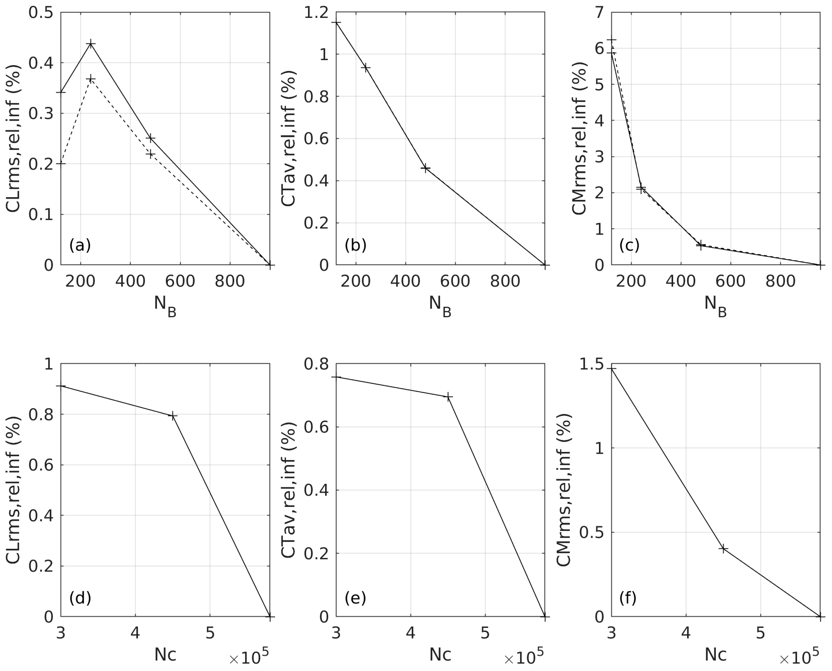
Turning into more details, we present in
Figure 19 a convergence study for a flapping foil in unbounded domain for the case studied in
Section 4.3. BEM convergence results with respect to the number of panels on the foil
and the size of the time step are plotted in
Figure 19a–c. The relevant errors in all cases are reasonably small and mean sectional lift coefficient converges faster while the moment coefficient is found to be the most demanding. Moreover, a grid independence study of RANSE calculations is presented in
Figure 19d–f using different grids (see
Table 1). In this case, the level of error remains below 0.8% for all cases for grid 3. It was decided to present the finer grid predictions in the preceded analysis for the reasons explained before and since the wake is better resolved.
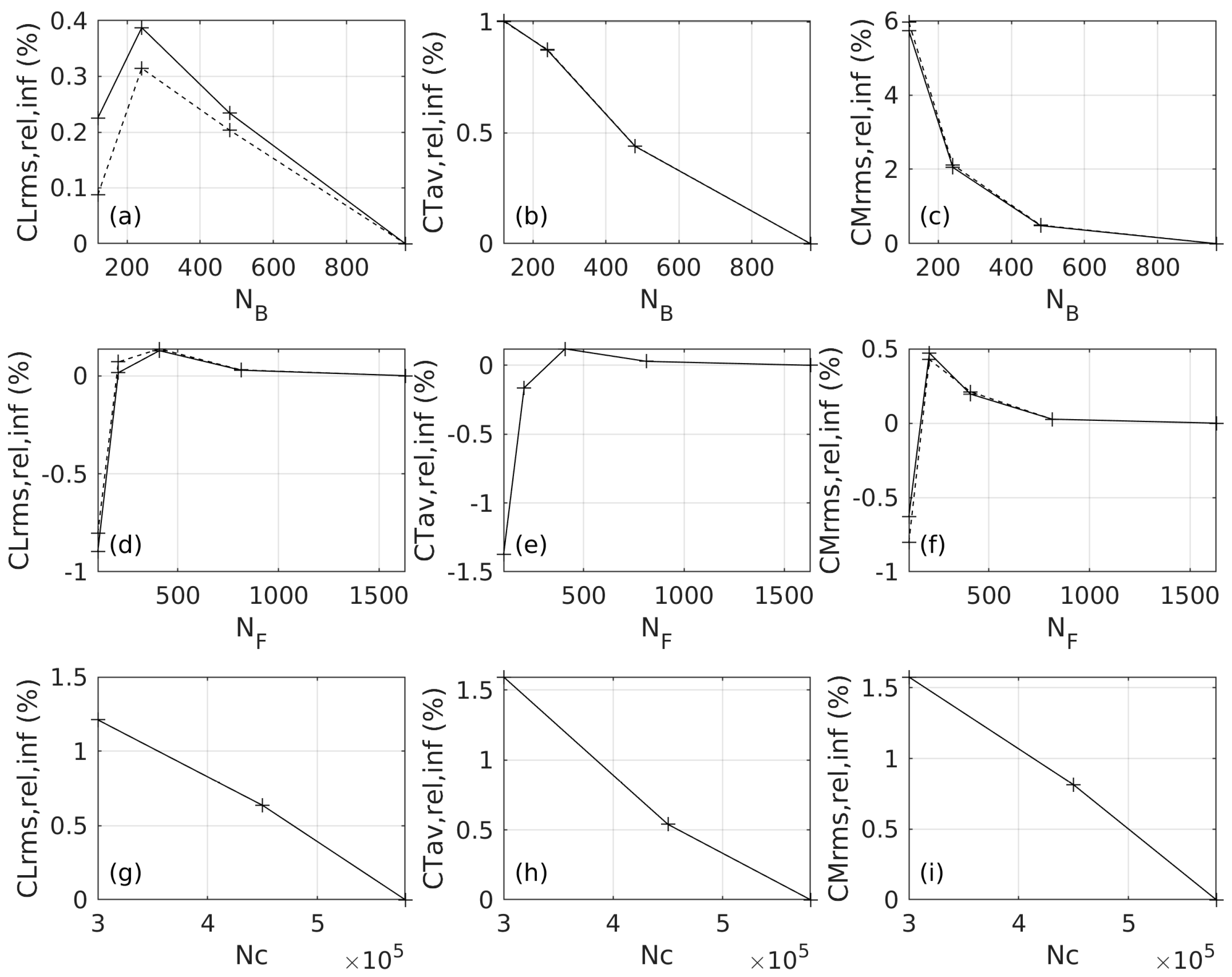
Furthermore, in
Figure 20 we present a convergence study for a flapping foil beneath the free surface for the case studied in
Section 4.4. BEM convergence results are plotted in
Figure 20a–c with respect to the number of panels on the foil
and the size of the time step and with respect to the number of panels on the free-surface boundary
in
Figure 20d–f, respectively. From the first case in
Figure 20a–c, we conclude that convergence characteristics are similar to the unbounded domain study as expected with slightly faster convergence. From the second case in
Figure 20d–f, it is seen that for the specific submergence ratio
the relative error reduces below 0.5% even for the coarser grids. However, we choose
to resolve adequately the most demanding case of
. A grid independence study of RANSE calculations is presented in
Figure 20g–i, using different grids according to
Table 1. The relative errors are very small, but the convergence is found to be slightly more demanding in comparison with the unbounded domain configuration due to the additional requirements imposed by the free-surface.
Finally, in
Figure 21, a convergence study for a flapping foil in waves for the case studied in
Section 4.2 is presented. BEM convergence with respect to the number of panels on the foil
and the size of the time step are presented in
Figure 21a–c and with respect to number of panels on the free-surface boundary
in
Figure 21d–f. The findings are similar with those from the preceded figures; however, as explained in the beginning of the present section, the effect of waves causes a variation of reduction by
,
, and
for the mean sectional values of
,
, and
, respectively, and not below
as in the case of free-surface effects. Therefore, if the interest is in the design of the flapping foil device extracting energy from the waves in mean submergence larger than 1 chord length and not to the resolution of the details of the free-surface effects, a coarser spatial and temporal grid could be adequate. The enhancement of the present method with incorporation of nonlinear effects associated with the free surface dynamics and the leading edge flow separation, as well as full treatment of 3D effects, are important future contributions, supporting also the design of the considered systems; see, e.g., [
20,
43].


