Fundamental limits of single anchor-based cooperative localization in millimeter wave systems

Abstract

Thanks to massive antenna arrays in millimeter wave communications, a much higher resolution can be achieved for the estimation of angle of arrival. By taking full advantage of beamforming capability and high angular resolution in millimeter wave systems, a single anchor is sufficient to obtain a good position estimation for agents by combining angle of arrival and time of arrival. In this paper, a single-anchor based cooperative localization is proposed for millimeter wave systems. Fundamental limits of cooperative localization with a single anchor is investigated, where all nodes are equipped with massive antenna arrays. Bounds of time-based range and position estimation are derived by Crámer-Rao bound in general multipath channels. For the single-anchor based cooperative localization, the structure of the fisher information matrix is investigated and the relationship between ranging accuracy and positioning accuracy is theoretically clarified. Numerical results demonstrate a consistency with theory behind the proposed millimeter wave’s cooperative localization network.

1 Introduction

As is well known, millimeter wave (mmWave) communication operates with the wide spectrum from 30 GHz to 300 GHz [1]. With a large available bandwidth and massive antenna arrays, mmWave bands are very promising and attractive in wireless communication [2]. The first standardized consumer radios were in the 60 GHz unlicensed band, where 2 GHz signal bandwidth is common. By virtue of this advantage, even though there exists a severe path loss in mmWave transmissions, the development of wireless communication in the 60 GHz band has been attracting plenty of attentions [3].

In addition to offering a large available bandwidth and massive antenna arrays, mmWave transmissions have a higher transmit power that leads to a higher signal noise ratio (SNR) compared with another probing signal with a large band named ultra wideband (UWB) ([4, 5]) in the frequency range of 3.1∼10.6 GHz. Consequently, mmWave has a tremendous potential for precise ranging and positioning and is capable of compensating for the drawbacks of satellite based positioning systems such as global positioning systems (GPS). So far, there have been many literatures conducting an investigation on mmWave localization. By measuring mmWave’s received signal strength (RSS), a meter-level positioning accuracy is obtained in [6]. Due to massive antenna arrays in mmWave communications, a much higher resolution is achieved for the estimation of angle of arrival (AOA) ([7–9]). Under this condition, a single anchor is sufficient for agents’ position estimation by using AOA and time of arrival (TOA), instead of multiple anchors involved in conventional localization networks ([10, 11]). This work has been extended to the case of multipath environments in ([12–14]), where the fundamental bounds for position and orientation estimation are derived. In [15], error bounds for uplink and downlink 3-dimensional (3D) localization in mmWave systems are derived based on single-anchor localization with uniform rectangular arrays. In indoor scenarios ([11, 16]), position and orientation error bounds are analyzed for single-anchor based 3D mmWave localization with a perfect single beam whose direction is assumed to be known, where only a single-path channel is considered. Our previous works investigate the multi-anchor based mmWave localization in static and dynamic multipath channels and achieve a millimeter-level (mm-level) positioning bound in the given mmWave localization systems ([17, 18]).

This paper proposes single-anchor based cooperative localization and investigates the fundamental limits on ranging and positioning in mmWave-based cooperative localization. Similar to ([19, 20]), the antenna array is regarded as a phased array because the signal bandwidth B is much smaller¹than the carrier frequency f_c, i.e., B≪f_c, although the band of mmWave is large ([3, 11]). Different from the existing literatures ([21, 22]) that achieve meter-level to centimeter-level positioning accuracy, we attempt to pursue a mm-level positioning accuracy and achieve a similar accuracy level as our previous work [19]. However, different from [19] that employs multiple anchors and adopts a large antenna array only for the anchor, this paper considers a single anchor based cooperative localization with the antenna array equipped for all nodes.

Figure 1 shows a genetic network topology for single anchor based cooperative localization. In the communication range of an agent, there is only a single anchor to be used for localization. For each anchor-agent connection pair, both TOA and AOA are measured; however, for each agent-agent connection pair, only the TOA is measured. In this paper, the fundamental limits of cooperative localization in mmWave systems are investigated, where a single anchor is utilized for resource saving. In communication networks, due to power control, the number of hearable anchors might be insufficient. Single anchor-based cooperative localization can eliminate this problem. Bounds of range, orientation, and position estimation are derived by Crámer-Rao bound (CRB) for general multipath channels. The structure of the fisher information matrix (FIM) is investigated, and the relationship between ranging accuracy and positioning accuracy is theoretically clarified. The contributions of this paper is summarized as follows:

• We propose mmWave-based cooperative localization with a single anchor to reduce the construction cost and overcome the hearability problem;

  Fig. 1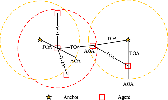

  

  Single anchor-based cooperative localization in mmWave systems

• In the proposed model associated with mmWave transmission and massive antenna arrays, we derive the CRB for range and orientation estimations for a single anchor and range estimation for agents;

• In the proposed model associated with mmWave transmission and massive antenna arrays, we analyze the FIM structure and derive the CRB for position estimation in single anchor-based cooperative localization;

• The close relationship between the bound for range estimation and that for position estimation is theoretically disclosed in single-anchor based cooperative localization.

The remaining of this paper is organized as follows. Section 2 introduces the system model and problem formulation. In Section 3, the bounds for range and orientation estimations are derived for single anchor, and the bound for range estimation is derived for agents. In Section 4, the FIM is structured and the bounds on position and orientation estimations are derived, where the bound of position estimation is associated with that of range estimation. Section 5 reports the numerical results, followed by conclusion in Section 6.

Notations: The superscripts [·]^∗,|·|, [·]^T, [·]⁻¹ and $\phantom {\dot {i}\!}[\cdot ]^{'}$ denote the conjugate, the modulus, the transpose, the inverse, and the first derivation of the argument, respectively; A≽B means that matrix A−B is positive semidefinite; [·]_i,j denotes the element at the i^th row and j^th column of its argument; [·]_r1:r2,c1:c2 denotes a submatrix composed of the rows r₁ to r₂ and the columns c₁ to c₂ of its argument; [·]_n×n,k denotes the kth n×n submatrix beginning from the element 2n(k−1)+1 on the diagonal of its argument; I_n denotes a n×n identity matrix, 1_m×n denotes a m×n matrix with all elements of 1 and 0_m×n denotes a m×n matrix with all elements of 0; A⊗B denotes the Kronecker product of A and B and A∘B denotes the Hadamard product of A and B; $\mathbb {E}_{\mathbf {v}}\{\cdot \}$ is the expectation operator with respect to the random vector v; tr(·) denotes the trace of a matrix.

2 System model and localization method

2.0.1 System model and problem formulation

Considering an mmWave localization system consisting of a single anchor with known coordinate p₀=(x₀,y₀) and K agents with unknown coordinates p_k=(x_k,y_k) to be localized, $k \in \{1,2,\cdots,K \} \overset {\Delta }{=} \mathcal {N}_{k}$, as shown in Fig. 2, where all nodes, indicating both the anchor and agents, are equipped with massive antenna array [23]. The node k has M_k antenna elements, $k \in \{0\} \cup \mathcal {N}_{k}$, where k=0 indicates the anchor and k>0 indicates the agent.

Fig. 2

Location-aware network

Even though it is argued that small-scale fading in line-of-sight (LOS) link of mmWave communications is not significant with strong beamforming and can thus be neglected ([1, 24]), we persist in considering a generic wireless propagation model that includes small-scale fading for LOS path. Furthermore, according to [24] and [25], mmWave signals are sensitive to blockage effects, which result in distinct differences in the LOS and non-LOS (NLOS) path losses. mmWave signals at 60 GHz band suffer much more as shown by the path loss model in ([25, 26]). Moreover, shadowing is another nonnegligible factor to affect mmWave signals. Nevertheless, in wireless localization based on TOA, we focus much more on the time of flight or equivalently the propagation delay than on the path loss. Consequently, in order to simplify the analysis, the path loss in this paper is comprehensively expressed as follows.

In Fig. 2, the red edge connecting a single anchor with each agent denotes the propagation from anchor to the agent, and the blue edge connecting two agents denotes the signal transmission between agents. After a simple geometric operation, the received signal matrix at node $k\in \mathcal {N}_{k}$ from node $j \in \{0\} \cup \mathcal {N}_{k} \backslash k, \mathbf {x}_{kj}(t) \in \mathbb {C}^{M_{k} \times 1}$, can be modeled as

$$ \small \mathbf{x}_{kj}(t) = \sum_{p=1}^{P_{kj}} \alpha_{kj}^{(p)} \mathbf{e}\left(\phi_{kj}^{(p)},\phi_{jk}^{(p)}\right) \mathbf{B}^{kj}(\boldsymbol{\phi}_{T}) \mathbf{s}\left(t - \tau_{kj}^{(p)}\right) + \mathbf{w}_{kj}(t), $$

(1)

where $\mathbf {e}\left (\phi _{kj}^{(p)},\phi _{jk}^{(p)}\right)=\mathbf {e}_{r}\left (\phi _{kj}^{(p)}\right) \mathbf {e}_{t}^{T}\left (\phi _{jk}^{(p)}\right) \in \mathbb {C}^{M_{k} \times M_{j}}$ is composed of antenna steering vector $\mathbf {e}_{t}\left (\phi _{jk}^{(p)}\right) \in \mathbb {C}^{M_{j} \times 1}$ and antenna response vector $\mathbf {e}_{r}\left (\phi _{kj}^{(p)}\right) \in \mathbb {C}^{M_{k} \times 1}$; $\mathbf {B}^{kj}(\boldsymbol {\phi }_{T}) \in \mathbb {C}^{M_{j} \times M_{b}}$ denotes the beamforming vectors with the targeted angle of transmission ϕ_T; $\phantom {\dot {i}\!}\mathbf {s}(t)=[s_{1}(t), s_{2}(t), \cdots, s_{M_{b}}(t)]^{T}$; P_kj denotes the number of multipath components; $\alpha _{kj}^{(p)}$ and $\tau _{kj}^{(p)}$ are the propagation amplitude and delay of the p^th path, respectively;

$$\tau_{kj}^{(p)} = \frac{1}{c}\left(\|\mathbf{p}_{j}-\mathbf{p}_{k}\|+b_{kj}^{(p)}\right)$$

with the light speed c and range bias $b_{kj}^{(p)} \geq 0$ in which the range bias is zero for the direct path; w_kj(t) represents the observation noise matrix, where each elements are modeled as additive white Gaussian processes with zero mean, variance of $\sigma _{w}^{2}$, and two-side power spectral density N₀/2.

Specifically, the received signal at antenna m of node k from node $j \in \{0\} \cup \mathcal {N}_{k} \backslash k$ can be obtained from (1)

$$\begin{array}{@{}rcl@{}} x_{kj}^{(m)}(t) &=& \sum_{p=1}^{P_{kj}} \alpha_{kj}^{(p)} e^{jg_{m}(\phi_{kj}^{(p)})} \mathbf{e}_{t}^{T}(\phi_{jk}^{(p)}) \mathbf{B}^{kj}(\boldsymbol{\phi}_{T}) \mathbf{s}(t - \tau_{kj}^{(p)}) \\ && + \mathbf{w}_{kj}^{(m)}(t), \end{array} $$

(2)

where $e^{jg_{m}(\phi _{kj}^{(p)})}$ is the steering phase of antenna m at the single anchor with respect to the p^th path.

2.0.2 Coperative localization with single anchor

A generic framework for cooperative localization has been proposed in [27] for wideband signals, where multiple anchors are considered for only delay estimation. Similar to [27], each agent in the cooperative network is localized by combining two components: single anchor’s localization and other agents’ cooperative localization.

In single anchor’s localization, each agent receives transmissions from the single anchor and then measures the angle as well as the propagation delay. The localization is then accomplished by using both AOA and TOA. In agents’ cooperative localization, each agent receives transmissions from all other hearable agents and then measures all propagation delays, where the localization is accomplished by using TOA or TDOA.

To sum up, in the proposed single anchor-based cooperative localization networks, the final localization is implemented by combining the AOA and TOA from single anchor and the entire TOAs from all hearable agents.

3 Bounds of range and orientation estimation

In this section, we derive the FIM and CRB for range estimation as well as for orientation estimation. Without loss of generality, we assume that each agent in localization networks knows the array orientation for itself and for the fixed anchor; however, it has no information about the array orientation for other agents.

3.1 FIM for range and orientation

Let θ_kj denote the parameters to be estimated during the propagation from node l to agent k, l≠k, which consists of the multipath delays, massive antenna array vectors and channel amplitudes. When j=0, we attempt to measure the range between the single anchor and agent k, and the orientation from the single anchor to agent k. When j≠0, we attempt to measure only the range between agents k and j. Therefore, we have

$$ \boldsymbol{\theta}_{kj} = \left\{ \begin{array}{rcl} \left[ \mathbf{l}_{kj}^{T}, \boldsymbol{\tau}_{kj}^{T}, \boldsymbol{\varphi}_{kj}^{T}, \boldsymbol{\alpha}_{kj}^{T} \right]^{T} & \text{for} & j = 0 \\ \left[ \boldsymbol{\tau}_{kj}^{T}, \boldsymbol{\varphi}_{kj}^{T}, \boldsymbol{\alpha}_{kj}^{T} \right]^{T} & \text{for} & j \neq 0, \end{array}\right. $$

(3)

where the special vector

$$\mathbf{l}_{kj} \overset{\Delta}{=} \left[ \tau_{kj}^{(1)}, \phi_{k0}^{(1)}\right]^{T}$$

contains unknown LOS parameters to be estimated for j=0;

$$ \boldsymbol{\tau}_{kj} \overset{\Delta}{=} \left\{ \begin{array}{rcl} \left[ \tau_{kj}^{(2)}, \tau_{kj}^{(3)}, \cdots, \tau_{kj}^{(P_{kj})}\right]^{T} & \text{for} & j = 0 \\ \left[ \tau_{kj}^{(1)}, \tau_{kj}^{(2)}, \tau_{kj}^{(3)}, \cdots, \tau_{kj}^{(P_{kj})}\right]^{T} & \text{for} & j \neq 0, \end{array}\right. $$

(4)

with $\tau _{kj}^{(1)}$ being the unique unknown parameter to be estimated for j≠0; $\boldsymbol {\varphi }_{kj} \overset {\Delta }{=} \left [ \boldsymbol {\phi }_{kj}^{T}, \boldsymbol {\phi }_{jk}^{T} \right ]^{T}$, in which

$$ \boldsymbol{\phi}_{kj} \overset{\Delta}{=} \left\{ \begin{array}{rcl} \left[ \phi_{kj}^{(2)}, \phi_{kj}^{(3)}, \cdots, \phi_{kj}^{(P_{kj})}\right]^{T} & \text{for} & j = 0 \\ \left[ \phi_{kj}^{(1)}, \phi_{kj}^{(2)}, \phi_{kj}^{(3)}, \cdots, \phi_{kj}^{(P_{kj})}\right]^{T} & \text{for} & j \neq 0, \end{array}\right. $$

$$ \boldsymbol{\phi}_{jk} \overset{\Delta}{=} \left\{ \begin{array}{rcl} \left[ \phi_{jk}^{(2)}, \phi_{jk}^{(3)}, \cdots, \phi_{jk}^{(P_{jk})}\right]^{T} & \text{for} & j = 0 \\ \left[ \phi_{jk}^{(1)}, \phi_{jk}^{(2)}, \phi_{jk}^{(3)}, \cdots, \phi_{jk}^{(P_{jk})}\right]^{T} & \text{for} & j \neq 0, \end{array}\right. $$

(5)

and

$$ \boldsymbol{\alpha}_{kj} \overset{\Delta}{=} \left[ \alpha_{kj}^{(1)}, \alpha_{kj}^{(2)}, \alpha_{kj}^{(3)}, \cdots, \alpha_{kj}^{(P_{kj})} \right]^{T} $$

(6)

for all $j \in \mathcal {N}_{k} \backslash k$. The observation vector is organized as

$$ \mathbf{x}_{kj} = \left[ \mathbf{x}_{kj}^{(1)}, \mathbf{x}_{kj}^{(2)}, \cdots, \mathbf{x}_{kj}^{(M_{k})} \right]^{T}, $$

(7)

where $\mathbf {x}_{kj}^{(m)}$ is obtained from the Karhunen-Loeve (KL) expansion of $\mathbf {x}_{kj}^{(m)}(t)$ in (2). Let $\hat {\boldsymbol {\theta }}_{kj}$ denote an unbiased estimator of the parameter vector θ_kj based on the observation vector x_kj.

The mean squared error (MSE) of $\hat {\boldsymbol {\theta }}_{kj}$ is bounded as [28]

$$ \mathbb{E}_{\mathbf{x}_{kj}|\boldsymbol{\theta}_{kj}} \left\{ (\hat{\boldsymbol{\theta}}_{kj} - \boldsymbol{\theta}_{kj})(\hat{\boldsymbol{\theta}}_{kj} - \boldsymbol{\theta}_{kj})^{T} \right\} \succeq \mathbf{J}_{\theta, kj}^{-1}, $$

(8)

where $\mathbb {E}_{\mathbf {x}_{kj}|\boldsymbol {\theta }_{kj}}[\cdot ]$ denotes the expectation operation parameterized by the unknown vector θ_kj, and J_θ,kj denotes the FIM for the parameter vector θ_kj. Let $\hat {\tau }_{kj}^{(1)}$ be an unbiased estimator of the parameter $\tau _{kj}^{(1)}$ that is the LOS delay.

Let $\hat {\phi }_{k0}^{(1)}$ be an unbiased estimator of $\phi _{k0}^{(1)}$. Thus, $\hat {\tau }_{kj}^{(1)}$ and $\hat {\phi }_{k0}^{(1)}$ are bounded respectively as

$$ \left\{ \begin{array}{rcl} \mathbb{E}_{\mathbf{x}_{kj}|\boldsymbol{\theta}_{kj}} \left\{ \left(\hat{\tau}_{kj}^{(1)} -\tau_{kj}^{(1)}\right)^{2} \right\} \geq \left[\mathbf{J}_{\theta, kj}^{-1} \right]_{1,1} & j \in \{0\} \cup \mathcal{N}_{k} \backslash k \\ \mathbb{E}_{\mathbf{x}_{kj}|\boldsymbol{\theta}_{kj}} \left\{ \left(\hat{\phi}_{kj}^{(1)} - \phi_{kj}^{(1)}\right)^{2} \right\} \geq \left[\mathbf{J}_{\theta, kj}^{-1} \right]_{2,2} & j = 0. \end{array}\right. $$

(9)

And the FIM J_θ,kj is defined as

$$ \mathbf{J}_{\theta, kj} \overset{\Delta}{=} \mathbb{E}_{\mathbf{x}_{kj}|\boldsymbol{\theta}_{kj}} \left\{ - \frac{\partial^{2} }{\partial \boldsymbol{\theta}_{kj} \partial \boldsymbol{\theta}_{kj}^{T}} \ln f\left(\mathbf{x}_{kj}|\boldsymbol{\theta}_{kj}\right) \right\}, $$

(10)

where f(x_kj|θ_kj) is the likelihood ratio of the random variable matrix x_kj

$$ f\left(\mathbf{x}_{kj}|\boldsymbol{\theta}_{kj}\right) = \prod_{m=1}^{M_{k}}f\left(\mathbf{x}_{kj}^{(m)}|\boldsymbol{\theta}_{kj}\right) $$

(11)

with

$$\begin{array}{@{}rcl@{}} && f\left(\mathbf{x}_{kj}^{(m)}|\boldsymbol{\theta}_{kj}\right) \varpropto \exp \left\{-\frac{1}{N_{0}} \int_{0}^{T} \left|x_{kj}^{(m)}(t) - \sum_{p=1}^{P_{kj}} \alpha_{kj}^{(p)} \right. \right. \\ && \left. \left.e^{jg_{m}\left(\phi_{kj}^{(p)}\right)} \mathbf{e}_{t}^{T}\left(\phi_{jk}^{(p)}\right) \mathbf{B}^{kj}(\boldsymbol{\phi}_{T}) \mathbf{s}\left(t - \tau_{kj}^{(p)}\right)\right|^{2} dt\right\}. \end{array} $$

3.2 Bounds on range and orientation for anchor-agent pair

We firstly consider range estimation and orientation estimation when agent k communicates with the single anchor (j=0). In this case, the FIM J_θ,k0 can be structured as

$$\begin{array}{@{}rcl@{}} \mathbf{J}_{\theta, k0}= \left[ \begin{array}{ccccc} \operatorname{F}_{\mathbf{l}_{k0}\mathbf{l}_{k0}} & \operatorname{F}_{\mathbf{l}_{k0} \boldsymbol{\tau}_{k0}} & \operatorname{F}_{\mathbf{l}_{k0},\boldsymbol{\phi}_{k0}} & \operatorname{F}_{\mathbf{l}_{k0} \boldsymbol{\alpha}_{k0}} \\ \operatorname{F}_{\boldsymbol{\tau}_{k0}\mathbf{l}_{k0}} & \operatorname{F}_{\boldsymbol{\tau}_{k0} \boldsymbol{\tau}_{k0}} & \operatorname{F}_{\boldsymbol{\tau}_{k0}\boldsymbol{\phi}_{k0}} & \operatorname{F}_{\boldsymbol{\tau}_{k0}\boldsymbol{\alpha}_{k0}} \\ \operatorname{F}_{\boldsymbol{\phi}_{k0} \mathbf{l}_{k0}} & \operatorname{F}_{\boldsymbol{\phi}_{k0}\boldsymbol{\tau}_{k0}} & \operatorname{F}_{\boldsymbol{\phi}_{k0}\boldsymbol{\phi}_{k0}} & \operatorname{F}_{\boldsymbol{\phi}_{k0}\boldsymbol{\alpha}_{k0}} \\ \operatorname{F}_{\boldsymbol{\alpha}_{k0} \mathbf{l}_{k0}} & \operatorname{F}_{\boldsymbol{\alpha}_{k0} \boldsymbol{\tau}_{k0}} & \operatorname{F}_{\boldsymbol{\alpha}_{k0} \boldsymbol{\phi}_{k0}} & \operatorname{F}_{\boldsymbol{\alpha}_{k0}\boldsymbol{\alpha}_{k0}} \end{array} \right], \end{array} $$

(12)

where $\operatorname {F}_{\mathbf {x}_{1} \mathbf {x}_{2}} \overset {\Delta }{=} \Re \left \{ \mathbb {E}_{\mathbf {x}_{kj}|\boldsymbol {\theta }_{kj}}\left \{ - \frac {\partial ^{2}}{\partial \mathbf {x}_{1} \partial \mathbf {x}_{2}} \ln f\left (\mathbf {x}_{kj}|\boldsymbol {\theta }_{kj}\right) \right \} \right \}$.

By referring to [17], all elements could be easily obtained via a straightforward algebraic transformation. It is evidently known that $\left [\mathbf {J}_{\theta, k0}^{-1} \right ]_{1,1}$ and $\left [\mathbf {J}_{\theta, k0}^{-1} \right ]_{2,2}$ are of interest even though the FIM J_θ,k0 has a higher dimension. By partitioning J_θ,k0 as

$$\begin{array}{@{}rcl@{}} \boldsymbol{\Upsilon}_{0,k0} &\overset{\Delta}{=}& \operatorname{F}_{\mathbf{l}_{k0}\mathbf{l}_{k0}} \in \mathbb{R}^{2 \times 2}, \\ \boldsymbol{\Upsilon}_{1,k0} &\overset{\Delta}{=}& \left[\operatorname{F}_{\mathbf{l}_{k0} \boldsymbol{\tau}_{k0}}, \operatorname{F}_{\mathbf{l}_{k0},\boldsymbol{\phi}_{k0}}, \operatorname{F}_{\mathbf{l}_{k0} \boldsymbol{\alpha}_{k0}} \right] \in \mathbb{R}^{2\times (4P_{k0}-2)}, \\ \boldsymbol{\Upsilon}_{2,k0} &\overset{\Delta}{=}& \left[ \begin{array}{cccc} \operatorname{F}_{\boldsymbol{\tau}_{k0} \boldsymbol{\tau}_{k0}} & \operatorname{F}_{\boldsymbol{\tau}_{k0}\boldsymbol{\phi}_{k0}} & \operatorname{F}_{\boldsymbol{\tau}_{k0}\boldsymbol{\alpha}_{k0}} \\ \operatorname{F}_{\boldsymbol{\phi}_{k0}\boldsymbol{\tau}_{k0}} & \operatorname{F}_{\boldsymbol{\phi}_{k0}\boldsymbol{\phi}_{k0}} & \operatorname{F}_{\boldsymbol{\phi}_{k0}\boldsymbol{\alpha}_{k0}} \\ \operatorname{F}_{\boldsymbol{\alpha}_{k0} \boldsymbol{\tau}_{k0}} & \operatorname{F}_{\boldsymbol{\alpha}_{k0} \boldsymbol{\phi}_{k0}} & \operatorname{F}_{\boldsymbol{\alpha}_{k0}\boldsymbol{\alpha}_{k0}}. \end{array} \right] \\ && \in \mathbb{R}^{(4P_{kj}-2)\times (4P_{kj}-2)}, \end{array} $$

(13)

we then have

$$ \mathbf{J}_{c, k0} = \boldsymbol{\Upsilon}_{0,k0} - \boldsymbol{\Upsilon}_{1,k0} \boldsymbol{\Upsilon}_{2,k0}^{-1} \boldsymbol{\Upsilon}_{1,k0}^{T}, $$

(14)

where J_c,k0 is defined as the Schur complement of J_θ,k0.

Fundamental bounds of range estimation $\hat {d}_{k0}$ and orientation estimation $\hat {\phi }_{k0}^{(1)}$ can thus be obtained as

$$ \left\{ \begin{array}{rcl} \sigma_{\hat{d}_{k0}}^{2} \geq c^{2} [(\boldsymbol{\Upsilon}_{0,k0} - \boldsymbol{\Upsilon}_{1,k0} \boldsymbol{\Upsilon}_{2,k0}^{-1} \boldsymbol{\Upsilon}_{1,k0}^{T})^{-1}]_{1,1} \overset{\Delta}{=} \mathcal{B}_{\hat{d}_{k0}} \\ \sigma_{\hat{\phi}_{k0}^{(1)}}^{2} \geq [(\boldsymbol{\Upsilon}_{0,k0} - \boldsymbol{\Upsilon}_{1,k0} \boldsymbol{\Upsilon}_{2,k0}^{-1} \boldsymbol{\Upsilon}_{1,k0}^{T})^{-1}]_{2,2} \overset{\Delta}{=} \mathcal{B}_{\hat{\phi}_{k0}^{(1)}}, \end{array}\right. $$

(15)

And the [Υ_0,k0]_1,1 can be obtained as

$$ [\boldsymbol{\Upsilon}_{0,k0}]_{1,1} = 8\pi^{2} M_{0} M_{k} \beta^{2} \mathsf{SNR}_{k0}^{(1)}, $$

(16)

where $\beta \overset {\Delta }{=} \left (\frac {\int _{-\infty }^{+\infty } f^{2}|S(f)|^{2} df}{\int _{-\infty }^{+\infty } |S(f)|^{2} df} \right)^{1/2}$ denotes the mean square bandwidth (MSB) [29] and $\mathsf {SNR}_{k0}^{(1)} \overset {\Delta }{=} \frac {|\alpha _{k0}^{(1)}|^{2} \int _{-\infty }^{+\infty } |S(f)|^{2} df}{N_{0}}$ denotes the received SNR of the LOS path at agent k from the single anchor.

3.2.1 Bounds on range estimation for agent-agent pair

We then consider range estimation between agents k and $j \in \mathcal {N}_{k} \backslash k$. In this case, the FIM J_θ,kj can be structured as

$$\begin{array}{@{}rcl@{}} \mathbf{J}_{\theta, kj}= \left[ \begin{array}{cccc} \operatorname{F}_{\mathbf{l}_{kj} \boldsymbol{\tau}_{kj}} & \operatorname{F}_{\mathbf{l}_{kj},\boldsymbol{\phi}_{kj}} & \operatorname{F}_{\mathbf{l}_{kj} \boldsymbol{\alpha}_{kj}} \\ \operatorname{F}_{\boldsymbol{\tau}_{kj} \boldsymbol{\tau}_{kj}} & \operatorname{F}_{\boldsymbol{\tau}_{kj}\boldsymbol{\phi}_{kj}} & \operatorname{F}_{\boldsymbol{\tau}_{kj}\boldsymbol{\alpha}_{kj}} \\ \operatorname{F}_{\boldsymbol{\phi}_{kj}\boldsymbol{\tau}_{kj}} & \operatorname{F}_{\boldsymbol{\phi}_{kj}\boldsymbol{\phi}_{kj}} & \operatorname{F}_{\boldsymbol{\phi}_{kj}\boldsymbol{\alpha}_{kj}} \\ \operatorname{F}_{\boldsymbol{\alpha}_{kj} \boldsymbol{\tau}_{kj}} & \operatorname{F}_{\boldsymbol{\alpha}_{kj} \boldsymbol{\phi}_{kj}} & \operatorname{F}_{\boldsymbol{\alpha}_{kj}\boldsymbol{\alpha}_{kj}} \end{array} \right], \end{array} $$

(17)

where all elements could be easily obtained via a straightforward algebraic transformation.

Similarly, $\left [\mathbf {J}_{\theta, kj}^{-1} \right ]_{1,1}$ is of interest although the FIM J_θ,kj has a higher dimension. By partitioning J_θ,kj as

$$\begin{array}{@{}rcl@{}} \Upsilon_{0,kj} &\overset{\Delta}{=}& \operatorname{F}_{\tau_{kj}^{(1)} \tau_{kj}^{(1)}} \in \mathbb{R}, \\ \boldsymbol{\Upsilon}_{1,kj} &\overset{\Delta}{=}& \left[\operatorname{F}_{\tau_{kj}^{(1)} \tilde{\boldsymbol{\tau}}_{kj}}, \operatorname{F}_{\tau_{kj}^{(1)} \boldsymbol{\phi}_{kj}}, \operatorname{F}_{\tau_{kj}^{(1)} \boldsymbol{\alpha}_{kj}} \right] \in \mathbb{R}^{1\times (4P_{kj}-1)}, \\ \boldsymbol{\Upsilon}_{2,kj} &\overset{\Delta}{=}& \left[ \begin{array}{cccc} \operatorname{F}_{\tilde{\boldsymbol{\tau}}_{kj} \boldsymbol{\tau}_{kj}} & \operatorname{F}_{\tilde{\boldsymbol{\tau}}_{kj}\boldsymbol{\phi}_{kj}} & \operatorname{F}_{\tilde{\boldsymbol{\tau}}_{kj}\boldsymbol{\alpha}_{kj}} \\ \operatorname{F}_{\boldsymbol{\phi}_{kj}\tilde{\boldsymbol{\tau}}_{kj}} & \operatorname{F}_{\boldsymbol{\phi}_{kj}\boldsymbol{\phi}_{kj}} & \operatorname{F}_{\boldsymbol{\phi}_{kj}\boldsymbol{\alpha}_{kj}} \\ \operatorname{F}_{\boldsymbol{\alpha}_{kj} \tilde{\boldsymbol{\tau}}_{kj}} & \operatorname{F}_{\boldsymbol{\alpha}_{kj} \boldsymbol{\phi}_{kj}} & \operatorname{F}_{\boldsymbol{\alpha}_{kj}\boldsymbol{\alpha}_{kj}}. \end{array} \right] \\ && \in \mathbb{R}^{(4P_{kj}-1)\times (4P_{kj}-1)}, \end{array} $$

(18)

where $\boldsymbol {\tau }_{kj} \overset {\Delta }{=} \left [ \tau _{kj}^{(2)}, \tau _{kj}^{(3)}, \cdots, \tau _{kj}^{(P_{kj})}\right ]^{T}$, i.e. $\tau _{kj}^{(1)}$ is excluded.

By defining J_c,kj as the Schur complement of the matrix J_θ,kj, we then have

$$ J_{c, kj} = \Upsilon_{0,kj} - \boldsymbol{\Upsilon}_{1,kj} \boldsymbol{\Upsilon}_{2,kj}^{-1} \boldsymbol{\Upsilon}_{1,kj}^{T}. $$

(19)

The bound on range estimation $\hat {d}_{kj}$ is similarly obtained as

$$ \sigma_{\hat{d}_{kj}}^{2} \geq c^{2} \left[\left(\Upsilon_{0,kj} - \boldsymbol{\Upsilon}_{1,kj} \boldsymbol{\Upsilon}_{2,kj}^{-1} \boldsymbol{\Upsilon}_{1,kj}^{T}\right)^{-1}\right]_{1,1} \overset{\Delta}{=} \mathcal{B}_{\hat{d}_{kj}}, $$

(20)

And the Υ_0,kj can be obtained as

$$ \Upsilon_{0,kj} = 8\pi^{2} M_{k} M_{j} \beta^{2} \mathsf{SNR}_{kj}^{(1)}, $$

(21)

where $\mathsf {SNR}_{kj}^{(1)} \overset {\Delta }{=} \frac {|\alpha _{kj}^{(1)}|^{2} \int _{-\infty }^{+\infty } |S(f)|^{2} df}{N_{0}}$ denotes the received SNR of the LOS path at agent k from agent j.

4 Bounds on position and orientation in single anchor-based cooperative localization

In this section, we investigated the structure of FIM for position estimation as well as for orientation estimation. Furthermore, we analyzed the contribution of single anchor’s localization and agents’ localization.

4.1 FIM and structure

4.1.1 FIM

By considering all transmissions from a single anchor and from K agents, the parameter vector to be estimated at agent k can be represented by

$$ \boldsymbol{\theta} = \left[ \mathbf{P}^{T}, \tilde{\boldsymbol{\theta}}_{1}^{T}, \tilde{\boldsymbol{\theta}}_{2}^{T}, \cdots, \tilde{\boldsymbol{\theta}}_{K}^{T} \right]^{T}, $$

(22)

where

$$ \mathbf{P} = \left[\mathbf{P}_{1}^{T}, \mathbf{P}_{2}^{T}, \cdots, \mathbf{P}_{K}^{T} \right]^{T} \ \ \text{with} \ \ \ \mathbf{P}_{k} = \left[\mathbf{p}_{k}^{T}, \phi_{k0}^{(1)}\right]^{T} $$

(23)

consists of positions of all agents and orientations of all nodes;

$$ \tilde{\boldsymbol{\theta}}_{k} = \left[\tilde{\boldsymbol{\theta}}_{k0}, \tilde{\boldsymbol{\theta}}_{k1}, \cdots, \tilde{\boldsymbol{\theta}}_{kj},\cdots, \tilde{\boldsymbol{\theta}}_{kK}\right]^{T} $$

(24)

with $j \in \{0\} \cup \mathcal {N}_{k} \backslash k$;

$$ \tilde{\boldsymbol{\theta}}_{kj} = \left[ \mathbf{b}_{kj}^{T}, \boldsymbol{\varphi}_{kj}^{T}, \boldsymbol{\alpha}_{kj}^{T} \right]^{T} $$

(25)

contains

$$\mathbf{b}_{kj} \overset{\Delta}{=} \left[ b_{kj}^{(2)}, b_{kj}^{(3)}, \cdots, b_{kj}^{(P_{kj})} \right]^{T} $$

and two other vectors φ_kj in (5) and α_kj in (6).

The observation vector x includes the received waveforms at all agents, which is represented by

$$\mathbf{x} = \left[ \mathbf{x}_{1}^{T}, \mathbf{x}_{2}^{T}, \cdots, \mathbf{x}_{K}^{T}\right]^{T},$$

where

$$\mathbf{x}_{k} = \left[ \mathbf{x}_{k1}, \mathbf{x}_{k2}, \cdots, \mathbf{x}_{kj}, \cdots, \mathbf{x}_{kK} \right]$$

with $j \in \{0\} \cup \mathcal {N}_{k} \backslash k$ and

$$\mathbf{x}_{kj} = \left[ \mathbf{x}_{kj}^{(1)}, \mathbf{x}_{kj}^{(2)}, \cdots, \mathbf{x}_{kj}^{(M_{k})} \right]^{T}.$$

And $\mathbf {x}_{kj}^{(m)}$, having the same expression as (7), is obtained from the Karhunen-Loeve (KL) expansion of $\mathbf {x}_{kj}^{(m)}(t)$ in (2). When node k cannot communicate with node j directly, the corresponding terms x_kj and x_jk disappear from x.

$\boldsymbol {\mathfrak {J}}_{\theta }$ is defined as the FIM of θ, so we have

$$ \boldsymbol{\mathfrak{J}}_{\theta} \overset{\Delta}{=} \mathbb{E}_{\mathbf{x}|\boldsymbol{\theta}} \left\{ - \frac{\partial^{2} }{\partial \boldsymbol{\theta} \partial \boldsymbol{\theta}^{T}} \ln f\left(\mathbf{x}|\boldsymbol{\theta}\right) \right\}, $$

(26)

where the overall likelihood ratio can be shown as

$$ f\left(\mathbf{x} | \boldsymbol{\theta} \right) = \prod_{k \in \mathcal{N}_{k}} \prod_{j \in {0} \cup \mathcal{N}_{k}\backslash k} \prod_{m=1}^{M_{k}} f\left(\mathbf{x}_{kj}^{(m)} | \tilde{\boldsymbol{\theta}}_{kj}\right). $$

(27)

Let $\hat {\mathbf {p}}_{k}=(\hat {x}_{k}, \hat {y}_{k})$ be an unbiased estimator of p_k=(x_k,y_k). Similarly, we have the MSE of $\hat {\mathbf {p}}_{k}$ and the orientation $\hat {\phi }_{k0}^{(1)}$ bounded as

$$ \left\{ \begin{array}{rcl} \mathbb{E}_{\mathbf{X}|\boldsymbol{\theta}} \left\{ (\hat{\mathbf{p}}_{k} - \mathbf{p}_{k})(\hat{\mathbf{p}}_{k} - \mathbf{p}_{k})^{T} \right\} \succeq \left[\boldsymbol{\mathfrak{J}}_{\theta}^{-1} \right]_{2\times 2, k} \\ \mathbb{E}_{\mathbf{x}|\boldsymbol{\theta}} \left\{ \left(\hat{\phi}_{k0}^{(1)} - \phi_{k0}^{(1)}\right)^{2} \right\} \geq \left[\boldsymbol{\mathfrak{J}}_{\theta}^{-1} \right]_{3k,3k} \end{array}\right. $$

(28)

in the proposed single anchor-based cooperative localization.

4.1.2 Structure of FIM

The log-likelihood function for single anchor-based cooperative localization can be expressed as

$$ \ln f\left(\mathbf{x} | \boldsymbol{\theta} \right) = \sum_{k \in \mathcal{N}_{k}} \sum_{j \in {0} \cup \mathcal{N}_{k}\backslash k} \ln f\left(\mathbf{x}_{kj} | \mathbf{P}_{k}, \mathbf{P}_{j}, \tilde{\boldsymbol{\theta}}_{kj} \right), $$

(29)

where $\mathbf {P}_{k} = \left [\mathbf {p}_{k}^{T}, \phi _{k0}^{(1)}\right ]^{T}$ is composed of the position of agent k and the orientation of the direct transmission from the single anchor to agent k, and $\tilde {\boldsymbol {\theta }}_{kj}$ denotes the vector of the channel parameters that are associated with nodes k and j. So, the FIM can be structured as

$$\begin{array}{@{}rcl@{}} \boldsymbol{\mathfrak{J}}_{\boldsymbol{\theta}} &=& \left[ \begin{array}{cccc} \operatorname{F}\left(\mathbf{P}, \mathbf{P} \right) & \operatorname{F}\left(\mathbf{P}, \tilde{\boldsymbol{\theta}}_{1} \right) & \cdots & \operatorname{F}\left(\mathbf{P}, \tilde{\boldsymbol{\theta}}_{K} \right) \\ \operatorname{F}\left(\tilde{\boldsymbol{\theta}}_{1}, \mathbf{P} \right) & \operatorname{F}\left(\tilde{\boldsymbol{\theta}}_{1}, \tilde{\boldsymbol{\theta}}_{1} \right) & & \mathbf{0} \\ \vdots & & \ddots & \\ \operatorname{F}\left(\tilde{\boldsymbol{\theta}}_{K}, \mathbf{P} \right) & \mathbf{0} & & \operatorname{F}\left(\tilde{\boldsymbol{\theta}}_{K}, \tilde{\boldsymbol{\theta}}_{K} \right) \end{array} \right], \\ \end{array} $$

(30)

where $\operatorname {F}\left (\mathbf {x}_{1}, \mathbf {x}_{2}\right) \overset {\Delta }{=} \mathbb {E}_{\mathbf {x}|\boldsymbol {\theta }}\left \{ - \frac {\partial ^{2}}{\partial \mathbf {x}_{1} \partial \mathbf {x}_{2}^{T}} \ln f\left (\mathbf {x}|\boldsymbol {\theta }\right) \right \}$, P denotes the vector which includes all P_k and $\tilde {\boldsymbol {\theta }}_{k}$ denotes the vector including all $\tilde {\boldsymbol {\theta }}_{kj}$ for $k \in \mathcal {N}_{k}$ and $j \in \{0\} \cup \mathcal {N}_{k} \backslash k$. The fact that $\operatorname {F}\left (\tilde {\boldsymbol {\theta }}_{k}, \tilde {\boldsymbol {\theta }}_{j} \right) = 0$ for k≠j is used here and the corresponding Schur complement can therefore be expressed as

$$ \boldsymbol{\mathfrak{J}}_{c}(\mathbf{P}) = \operatorname{F}\left(\mathbf{P}, \mathbf{P} \right) - \operatorname{F}\left(\mathbf{P}, \tilde{\boldsymbol{\theta}} \right) \left[ \operatorname{F}\left(\tilde{\boldsymbol{\theta}}, \tilde{\boldsymbol{\theta}} \right) \right]^{-1} \operatorname{F}\left(\mathbf{P}, \tilde{\boldsymbol{\theta}} \right)^{T}, $$

(31)

where $\operatorname {F}\left (\mathbf {P}, \tilde {\boldsymbol {\theta }} \right) \overset {\Delta }{=} \left [ \operatorname {F}\left (\mathbf {P}, \tilde {\boldsymbol {\theta }}_{1} \right), \operatorname {F}\left (\mathbf {P}, \tilde {\boldsymbol {\theta }}_{2} \right), \cdots, \operatorname {F}\left (\mathbf {P}, \tilde {\boldsymbol {\theta }}_{K} \right)\right ]$; $\operatorname {F}\left (\tilde {\boldsymbol {\theta }}, \tilde {\boldsymbol {\theta }} \right) \overset {\Delta }{=} \text {diag} \left \{ \operatorname {F}\left (\tilde {\boldsymbol {\theta }}_{1}, \tilde {\boldsymbol {\theta }}_{1} \right), \operatorname {F}\left (\tilde {\boldsymbol {\theta }}_{2}, \tilde {\boldsymbol {\theta }}_{2} \right), \cdots, \operatorname {F}\left (\tilde {\boldsymbol {\theta }}_{K}, \tilde {\boldsymbol {\theta }}_{K} \right) \right \}$.

Proposition 1

$\boldsymbol {\mathfrak {J}}_{c}(\mathbf {P})$, including all agent’s positions $\hat {\mathbf {p}}_{k}=(\hat {x}_{k}, \hat {y}_{k})$ and orientations $\hat {\phi }_{k0}^{(1)}$ for all $k \in \mathcal {N}_{k}$, can be divided into two independent components, where one component originates from the contribution of single-anchor localization and the other is from the contribution of all hearable agents’ cooperative localization.

Proof

By referring to [27], it is not difficult to find

$$\begin{array}{@{}rcl@{}} \boldsymbol{\mathfrak{J}}_{c}(\mathbf{P}) &=& \underbrace { \sum_{k \in \mathcal{N}_{k}} \operatorname{F}_{k0}\left(\mathbf{P}, \mathbf{P} \right) - \boldsymbol{\Phi}_{k0}\left(\mathbf{P}, \tilde{\boldsymbol{\theta}}_{k0}, \mathbf{P} \right) }_{\text{From single-anchor localization}} \\ & -& \underbrace { \sum_{k \in \mathcal{N}_{k}} \sum_{j \in \cup \mathcal{N}_{k} \backslash k} \operatorname{F}_{kj}\left(\mathbf{P}, \mathbf{P} \right) - \boldsymbol{\Phi}_{kj}\left(\mathbf{P}, \tilde{\boldsymbol{\theta}}_{kj}, \mathbf{P} \right)}_{\text{From agents' cooperative localization}} \\ &\triangleq& \boldsymbol{\mathfrak{J}}_{c, N}(\mathbf{P}) + \boldsymbol{\mathfrak{J}}_{c, G}(\mathbf{P}), \end{array} $$

(32)

where $\operatorname {F}_{kj}\left (\mathbf {x}_{1},\mathbf {x}_{2}\right) \triangleq \mathbb {E}_{\mathbf {x}|\boldsymbol {\theta }}\left \{ - \frac {\partial ^{2}}{\partial \mathbf {x}_{1} \partial \mathbf {x}_{2}} \ln f\left (\mathbf {x}_{kj}|\mathbf {P}_{k}, \mathbf {P}_{j}, \tilde {\boldsymbol {\theta }}_{kj}\right) \right \}$; $\boldsymbol {\Phi }_{kj}\left (\mathbf {x}_{1}, \mathbf {x}_{2}, \mathbf {x}_{3} \right) \triangleq \operatorname {F}_{kj}\left (\mathbf {x}_{1}, \mathbf {x}_{2} \right) \left [ \operatorname {F}_{kj}\left (\mathbf {x}_{2}, \mathbf {x}_{2} \right) \right ]^{-1}\operatorname {F}_{kj}\left (\mathbf {x}_{2}, \mathbf {x}_{3} \right)$.

Single anchor’s localization generates

$$ \boldsymbol{\mathfrak{J}}_{c, N}(\mathbf{P}) = \text{diag} \left\{ \boldsymbol{\mathfrak{J}}_{c, k0}(\mathbf{P}_{1}), \boldsymbol{\mathfrak{J}}_{c, k0}(\mathbf{P}_{2}), \cdots, \boldsymbol{\mathfrak{J}}_{c, k0}(\mathbf{P}_{K}) \right\}, $$

(33)

where $\boldsymbol {\mathfrak {J}}_{c, k0}$ represents single anchor’s localization for each agent. And all agent’s cooperative localization generates $\boldsymbol {\mathfrak {J}}_{c, G}(\mathbf {P})$ as in (34), where $\boldsymbol {\mathfrak {J}}_{c, kj}$ is associated with agent k and agent j. All $\boldsymbol {\mathfrak {J}}_{c, k0}$ in (33) and $\boldsymbol {\mathfrak {J}}_{c, kj}$ in (34) will be found out in the following subsections. □

$$\begin{array}{@{}rcl@{}} \begin{aligned} \boldsymbol{\mathfrak{J}}_{c,G}(\mathbf{P}) &=& \left[ \begin{array}{ccccccc} \sum_{j \in \mathcal{N}_{k} \backslash \{1\}} \boldsymbol{\mathfrak{J}}_{c, 1j}(\mathbf{p}_{1}) & 0 & -\boldsymbol{\mathfrak{J}}_{c, 12}(\mathbf{p}_{1}) & 0 & \cdots & -\boldsymbol{\mathfrak{J}}_{c, 1K}(\mathbf{p}_{1}) & 0 \\ 0 & 0 & 0 & 0 & \cdots & 0 & 0 \\ -\boldsymbol{\mathfrak{J}}_{c, 21}(\mathbf{p}_{2}) & 0 & \sum_{j \in \mathcal{N}_{k} \backslash \{2\}} \boldsymbol{\mathfrak{J}}_{c, 2j}(\mathbf{p}_{2}) & 0 & \cdots & -\boldsymbol{\mathfrak{J}}_{c, 2K}(\mathbf{p}_{2}) & 0 \\ 0 & 0 & 0 & 0 & \cdots & 0 & 0 \\ \vdots & \vdots & & \ddots & & & \\ -\boldsymbol{\mathfrak{J}}_{c, K1}(\mathbf{p}_{K}) & 0 & -\boldsymbol{\mathfrak{J}}_{c, K2}(\mathbf{p}_{K}) & 0 & \cdots & \sum_{j \in \mathcal{N}_{k} \backslash \{K\}} \boldsymbol{\mathfrak{J}}_{c, Kj}(\mathbf{p}_{K}) & 0 \\ 0 & 0 & 0 & 0 & \cdots & 0 & 0 \end{array} \right]_{3K \times 3K}, \end{aligned} \end{array} $$

(34)

4.2 Single anchor’s localization

4.2.1 Contribution of single anchor’s localization $\boldsymbol {\mathfrak {J}}_{c, n}(\mathbf {P})$

In order to find the details of $\boldsymbol {\mathfrak {J}}_{c, n}(\mathbf {P})$ and associate position estimation with range estimation, we further consider a parameter transformation from $\boldsymbol {\rho }_{k} = \left [ \mathbf {p}_{k}^{T}, \phi _{k0}^{(1)}, \tilde {\boldsymbol {\theta }}_{k0}^{T} \right ]^{T}$ to η_k=θ_k0, where $\tilde {\boldsymbol {\theta }}_{k0}$ is given in (24)-(25) and θ_k0 is given in (3). So, we have the FIM $\phantom {\dot {i}\!}\boldsymbol {\mathfrak {J}}_{\boldsymbol {\rho }_{k}}$ as

$$ \boldsymbol{\mathfrak{J}}_{\boldsymbol{\rho}_{k}} = \boldsymbol{\Xi} \mathbf{J}_{\boldsymbol{\eta}_{k}} \boldsymbol{\Xi}^{T}, $$

(35)

where $\phantom {\dot {i}\!}\boldsymbol {\mathfrak {J}}_{\boldsymbol {\rho }_{k}}$ and $\phantom {\dot {i}\!}\mathbf {J}_{\boldsymbol {\eta }_{k}}$ are the FIMs for the position’s parameter vector ρ_k and the range’s parameter vector η_k respectively, and Ξ is the Jacobian matrix for the transformation.

Thus, we have the diagonal block matrix

$$ \mathbf{J}_{\boldsymbol{\eta}_{k}}= \mathbf{J}_{\boldsymbol{\theta}, k0}, $$

(36)

where J_θ,k0 is given in (12). And,

$$ \boldsymbol{\Xi}= \frac{\partial \boldsymbol{\eta}_{k}}{\partial \boldsymbol{\rho}_{k}}= \left[ \begin{array}{c} \mathbf{H}_{k0} \\ \mathbf{D}_{k0} \\ \mathbf{Q}_{k0} \end{array} \right], $$

(37)

where

$$\begin{array}{@{}rcl@{}} \mathbf{H}_{k0} &=& \left[ \frac{1}{c}\mathbf{q}_{k0}, \tilde{\mathbf{q}}_{k0}, \frac{1}{c} \mathbf{q}_{k0} \otimes \mathbf{u}_{k0}, \mathbf{0}_{2 \times 2P_{k0}-1}, \mathbf{0}_{2 \times P_{k0}} \right] \\ && \in \mathbb{R}^{2\times 4P_{k0}}, \end{array} $$

(38)

with

$$\begin{array}{@{}rcl@{}} \mathbf{q}_{k0}&=&\left[\cos \phi_{k0}^{(1)}, \sin \phi_{k0}^{(1)} \right]^{T}, \\ \tilde{\mathbf{q}}_{k0} &=& \left[-\sin \phi_{k0}^{(1)}, \cos \phi_{k0}^{(1)} \right]^{T}, \\ \mathbf{u}_{k0} &=& \underbrace{\left[ 1, 1, \cdots, 1 \right]}_{P_{k0}-1}; \end{array} $$

(39)

$$ \mathbf{D}_{k0} = \left[ 0, 1, \mathbf{0}_{1 \times P_{k0}-1}, \mathbf{0}_{1 \times 2P_{k0}-1}, \mathbf{0}_{1 \times P_{k0}} \right] \in \mathbb{R}^{1 \times 4P_{k0}}; $$

(40)

and

$$\begin{array}{@{}rcl@{}} \mathbf{Q}_{k0}&=& \left[ \begin{array}{cccc} \mathbf{0}_{(P_{k0}-1)\times 2} & \mathbf{I}_{P_{k0}-1} & & \mathbf{0} \\ \mathbf{0}_{(2P_{k0}-1)\times 2} & & \mathbf{I}_{2P_{k0}-1} & \\ \mathbf{0}_{(P_{k0})\times 2} & \mathbf{0} & & \mathbf{I}_{P_{k0}} \end{array} \right] \\ &=& [\mathbf{0}, \mathbf{I}_{4P_{k0}-2} ] \in \mathbb{R}^{(4P_{k0}-2)\times (4P_{k0})}. \end{array} $$

(41)

By substituting (38) through (41) into (37) and substituting (37), (36) into (35), $\boldsymbol {\mathfrak {J}}_{\boldsymbol {\rho }_{k}}$ can be partitioned and represented as

$$ \boldsymbol{\mathfrak{J}}_{\boldsymbol{\rho}_{k}} = \left[ \begin{array}{cc} \boldsymbol{\beth}_{0} & \boldsymbol{\beth}_{1} \\ \boldsymbol{\beth}_{1}^{T} & \boldsymbol{\beth}_{2} \end{array} \right], $$

(42)

where

$$\begin{array}{@{}rcl@{}} \boldsymbol{\beth}_{0} &=& \left[ \begin{array}{cc} \mathbf{H}_{k0} \mathbf{J}_{\boldsymbol{\theta},k0} \mathbf{H}_{k0}^{T} & \mathbf{H}_{k0} \mathbf{J}_{\boldsymbol{\theta},k0} \mathbf{D}_{k0}^{T} \\ \mathbf{D}_{k0} \mathbf{J}_{\boldsymbol{\theta},k0} \mathbf{H}_{k0}^{T} & \mathbf{D}_{k0} \mathbf{J}_{\boldsymbol{\theta},k0} \mathbf{D}_{k0}^{T} \end{array} \right] \in \mathbb{R}^{3\times 3} \\ \boldsymbol{\beth}_{1} &=& \left[ \begin{array}{c} \mathbf{H}_{k0} \mathbf{J}_{\boldsymbol{\theta},k0} \mathbf{Q}_{k0}^{T} \\ \mathbf{D}_{k0} \mathbf{J}_{\boldsymbol{\theta},k0} \mathbf{Q}_{k0}^{T} \end{array} \right] \\ \boldsymbol{\beth}_{2} &=& \mathbf{Q}_{k0} \mathbf{J}_{\boldsymbol{\theta},k0} \mathbf{Q}_{k0}^{T}. \end{array} $$

(43)

Let $\mathbf {H}_{k0}= \left [ \frac {1}{c}\check {\mathbf {q}}_{k0}, \check {\mathbf {H}}_{k0}\right ]$ and $\mathbf {D}_{k0} = \left [ \check {\mathbf {D}}_{k0}, \mathbf {0} \right ]$, where $\check {\mathbf {q}}_{k0} = \left [ \mathbf {q}_{k0}, c\tilde {\mathbf {q}}_{k0} \right ]$ and $\check {\mathbf {D}}_{k0} = [0, 1]$. By using (13), we further have

$$\begin{array}{@{}rcl@{}} \mathbf{H}_{k0} \mathbf{J}_{\boldsymbol{\theta},k0} \mathbf{H}_{k0}^{T} &=& \frac{1}{c^{2}} \check{\mathbf{q}}_{k0} \Upsilon_{0,k0} \check{\mathbf{q}}_{k0}^{T} + \frac{1}{c} \check{\mathbf{H}}_{k0} \boldsymbol{\Upsilon}_{1,k0}^{T} \check{\mathbf{q}}_{k0}^{T} \\ && + \frac{1}{c} \check{\mathbf{q}}_{k0} \boldsymbol{\Upsilon}_{1,k0} \check{\mathbf{H}}_{k0}^{T} + \check{\mathbf{H}}_{k0} \boldsymbol{\Upsilon}_{2,k0} \check{\mathbf{H}}_{k0}^{T} \\ \mathbf{H}_{k0} \mathbf{J}_{\boldsymbol{\theta},k0} \mathbf{D}_{k0}^{T} &=& \frac{1}{c} \check{\mathbf{q}}_{k0} \boldsymbol{\Upsilon}_{0,k0} \check{\mathbf{D}}_{k0}^{T} + \check{\mathbf{H}}_{k0} \boldsymbol{\Upsilon}_{1,k0}^{T} \check{\mathbf{D}}_{k0}^{T} \\ \mathbf{D}_{k0} \mathbf{J}_{\boldsymbol{\theta},k0} \mathbf{D}_{k0}^{T} &=& \check{\mathbf{D}}_{k0} \boldsymbol{\Upsilon}_{0,k0} \check{\mathbf{D}}_{k0}^{T} \\ \mathbf{H}_{k0} \mathbf{J}_{\boldsymbol{\theta},k0} \mathbf{Q}_{k0}^{T} &=& \frac{1}{c} \check{\mathbf{q}}_{k0} \boldsymbol{\Upsilon}_{1,k0} + \check{\mathbf{H}}_{k0} \boldsymbol{\Upsilon}_{2,k0} \\ \mathbf{D}_{k0} \mathbf{J}_{\boldsymbol{\theta},k0} \mathbf{Q}_{k0}^{T}&=&\left[ \mathbf{Q}_{k0} \mathbf{J}_{\boldsymbol{\theta},k0} \mathbf{D}_{k0}^{T} \right]^{T} = \mathbf{0} \\ \mathbf{Q}_{k0} \mathbf{J}_{\boldsymbol{\theta},k0} \mathbf{Q}_{k0}^{T} &=& \boldsymbol{\Upsilon}_{2,k0}. \end{array} $$

(44)

Accordingly, the Schur complement of matrix $\boldsymbol {\beth }_{2}$, which is actually $\boldsymbol {\mathfrak {J}}_{c, k0}(\mathbf {P}_{k})$, can be associated with the performance of range estimation J_c,k0 in (14) as

$$ \boldsymbol{\mathfrak{J}}_{c, k0}(\mathbf{P}_{k}) = \left[ \begin{array}{cc} \frac{1}{c^{2}} \check{\mathbf{q}}_{k0} \mathbf{J}_{c, k0} \check{\mathbf{q}}_{k0}^{T} & \boldsymbol{\zeta}_{k0} \\ \boldsymbol{\zeta}_{k0}^{T} & \check{\mathbf{D}}_{k0} \boldsymbol{\Upsilon}_{0,k0} \check{\mathbf{D}}_{k0}^{T} \end{array} \right], $$

(45)

where $\boldsymbol {\zeta }_{k0}=\frac {1}{c} \check {\mathbf {q}}_{k0} \boldsymbol {\Upsilon }_{0,k0} \check {\mathbf {D}}_{k0}^{T} + \check {\mathbf {H}}_{k0} \boldsymbol {\Upsilon }_{1,k0}^{T} \check {\mathbf {D}}_{k0}^{T}$.

4.2.2 Effect of orientation to position estimation $\boldsymbol {\mathfrak {J}}_{c, k0}(\mathbf {P}_{k})$

By applying a similar partitioning as (42)-(43) on (45), $\boldsymbol {\mathfrak {J}}_{c, k0}(\mathbf {P}_{k})$ can be obtained as

$$\begin{array}{@{}rcl@{}} \boldsymbol{\mathfrak{J}}_{c, k0}(\mathbf{p}_{k}) &=& \frac{1}{c^{2}} \check{\mathbf{q}}_{k0} \mathbf{J}_{c, k0} \check{\mathbf{q}}_{k0}^{T} - \tilde{\mathbf{q}}_{k0} \tilde{\mathbf{q}}_{k0}^{T} [\boldsymbol{\Upsilon}_{0,k0}]_{2, 2} \\ && - \frac{1}{c^{2}} \tilde{\mathbf{q}}_{k0} \tilde{\mathbf{q}}_{k0}^{T} \circ \boldsymbol{\epsilon}_{k0}, \end{array} $$

(46)

where

$$\boldsymbol{\epsilon}_{k0}=\left[ \begin{array}{cc} \boldsymbol{\chi}_{1,2}^{2} & \boldsymbol{\chi}_{1,2} \boldsymbol{\chi}_{2,2} \\ \boldsymbol{\chi}_{1,2}\boldsymbol{\chi}_{2,2} & \boldsymbol{\chi}_{2,2}^{2} \end{array} \right]$$

with $\boldsymbol {\chi } = \bar {\mathbf {I}}_{k0} \boldsymbol {\Upsilon }_{1,k0}^{T}$ being a 2×2 matrix and $\bar {\mathbf {I}}_{k0}$ satisfying $\bar {\mathbf {I}}_{k0} = \left [ \mathbf {1}_{2\times (P_{k0}-1)}, \mathbf {0}_{2\times (3P_{k0}-1)} \right ]$.

By considering the definition of Υ_1,k0 in (13), we further have

$$ \boldsymbol{\chi} = \sum_{p=2}^{P_{kj}}\left[ \begin{array}{cc} \operatorname{F}_{\tau_{k0}^{(1)} \tau_{k0}^{(p)}} & \operatorname{F}_{\phi_{k0}^{(1)} \tau_{k0}^{(p)}} \\ \operatorname{F}_{\tau_{k0}^{(1)} \tau_{k0}^{(p)}} & \operatorname{F}_{\phi_{k0}^{(1)} \tau_{k0}^{(p)}} \end{array} \right] $$

(47)

and

$$ \boldsymbol{\epsilon}_{k0}= \left(\sum_{p=2}^{P_{kj}} \operatorname{F}_{\phi_{k0}^{(1)} \tau_{k0}^{(p)}}\right)^{2} \mathbf{1}_{2 \times 2}. $$

(48)

Consequently, $\boldsymbol {\mathfrak {J}}_{c, k0}(\mathbf {P}_{k})$ can be obtained as

$$\begin{array}{@{}rcl@{}} \boldsymbol{\mathfrak{J}}_{c, k0}(\mathbf{p}_{k}) &=& \frac{1}{c^{2}} \check{\mathbf{q}}_{k0} \mathbf{J}_{c, k0} \check{\mathbf{q}}_{k0}^{T} \\ & -& \tilde{\mathbf{q}}_{k0} \tilde{\mathbf{q}}_{k0}^{T} \left[ \operatorname{F}_{\phi_{k0}^{(1)} \phi_{k0}^{(1)}} + \frac{\left(\sum_{p=2}^{P_{kj}} \operatorname{F}_{\phi_{k0}^{(1)} \tau_{k0}^{(p)}}\right)^{2}}{c^{2}} \right] \\ &=& \frac{1}{c^{2}} \check{\mathbf{q}}_{k0} \mathbf{J}_{c, k0} \check{\mathbf{q}}_{k0}^{T} -\tilde{\mathbf{q}}_{k0} \tilde{\mathbf{q}}_{k0}^{T} \operatorname{F}_{\phi_{k0}^{(1)} \phi_{k0}^{(1)}}, \end{array} $$

(49)

because $\phi _{k0}^{(1)}$ and $\tau _{k0}^{(p)}$ are mutually independent, where p∈{2,3,⋯,P_kj}.

4.3 Agents’ localization: $\boldsymbol {\mathfrak {J}}_{c, G}(\mathbf {P})$

In order to find the details of FIM to be associated with the range estimation, we further consider a parameter transformation from $\boldsymbol {\rho }_{k} = \left [ \mathbf {p}_{k}^{T}, \tilde {\boldsymbol {\theta }}_{k1}^{T}, \tilde {\boldsymbol {\theta }}_{k2}^{T}, \cdots, \tilde {\boldsymbol {\theta }}_{kj}^{T},\cdots, \tilde {\boldsymbol {\theta }}_{kK}^{T} \right ]^{T}$ to $\boldsymbol {\eta }_{k} = \left [ \boldsymbol {\theta }_{k1}^{T}, \boldsymbol {\theta }_{k2}^{T}, \cdots, \boldsymbol {\theta }_{kj}^{T}, \cdots, \boldsymbol {\theta }_{kK}^{T} \right ]^{T}$, where $\tilde {\boldsymbol {\theta }}_{kj}$ is given in (24)-(25) and θ_kj is given in (3). So, we have the FIM $\phantom {\dot {i}\!}\mathbf {J}_{\boldsymbol {\rho }_{k}}$ as

$$ \boldsymbol{\mathfrak{J}}_{\boldsymbol{\rho}_{k}} = \boldsymbol{\Xi} \mathbf{J}_{\boldsymbol{\eta}_{k}} \boldsymbol{\Xi}^{T}, $$

(50)

where $\phantom {\dot {i}\!}\boldsymbol {\mathfrak {J}}_{\boldsymbol {\rho }_{k}}$ and $\phantom {\dot {i}\!}\mathbf {J}_{\boldsymbol {\eta }_{k}}$ are similarly the FIMs for the parameter vector ρ_k and η_k respectively, and Ξ is the Jacobian matrix for the transformation.

Thus, we have the diagonal block matrix

$$ \mathbf{J}_{\boldsymbol{\eta}_{k}}= \text{diag} \left\{\mathbf{J}_{\boldsymbol{\theta}, k0}, \mathbf{J}_{\boldsymbol{\theta}, k1},\cdots, \mathbf{J}_{\boldsymbol{\theta}, kj},\cdots, \mathbf{J}_{\boldsymbol{\theta}, kK} \right\}, $$

(51)

where J_θ,kj is given in (17).

And,

$$ \boldsymbol{\Xi}= \frac{\partial \boldsymbol{\eta}_{k}}{\partial \boldsymbol{\rho}_{k}}= \left[ \begin{array}{cccc} \mathbf{H}_{k1} & \mathbf{H}_{k2} & \cdots & \mathbf{H}_{kK} \\ \mathbf{Q}_{k1} & & & \mathbf{0} \\ & \mathbf{Q}_{k2} & & \\ & & \ddots & \\ \mathbf{0} & & &\mathbf{Q}_{kK} \end{array} \right], $$

(52)

where

$$ \mathbf{H}_{kj} = \left[ \frac{1}{c}\mathbf{q}_{kj}\otimes \mathbf{u}_{kj}, \mathbf{0}, \mathbf{0}, \mathbf{0} \right] \in \mathbb{R}^{2\times 4P_{kj}}, $$

(53)

with

$$\begin{array}{@{}rcl@{}} \mathbf{q}_{kj}&=&\left[\cos \phi_{kj}^{(1)}, \sin \phi_{kj}^{(1)} \right]^{T}, \\ \mathbf{u}_{kj} &=& \underbrace{\left[ 1, 1, \cdots, 1 \right]}_{P_{kj}}, \end{array} $$

(54)

and

$$ \mathbf{Q}_{kj}= \left[ \begin{array}{ccc} \mathbf{0} & \mathbf{I}_{P_{kj}-1} & \mathbf{0} \\ 0 & 0 & \mathbf{I}_{3P_{kj}} \end{array} \right] = [\mathbf{0}, \mathbf{I}_{4P_{kj}-1} ] \in \mathbb{R}^{4P_{kj}\times 4P_{kj}}. \ \ \ $$

(55)

By substituting (53) through (55) into (52) and substituting (51), (52) into (49), $\boldsymbol {\mathfrak {J}}_{\boldsymbol {\rho }_{k}}$ can be partitioned and represented as

$$ \boldsymbol{\mathfrak{J}}_{\boldsymbol{\rho}_{k}} = \left[ \begin{array}{cc} \boldsymbol{\beth}_{0} & \boldsymbol{\beth}_{1} \\ \boldsymbol{\beth}_{1}^{T} & \boldsymbol{\beth}_{2} \end{array} \right], $$

(56)

where all elements and the Schur complement of the matrix can be easily obtained by referring to Section 4B. The Schur complement of the matrix $\boldsymbol {\beth }_{2}$, which is actually $\boldsymbol {\mathfrak {J}}_{c, kj}(\mathbf {p}_{k})$, can be associated with range estimation J_c,kj in (19) as

$$ \boldsymbol{\mathfrak{J}}_{c, kj}(\mathbf{p}_{k}) = \frac{1}{c^{2}} \sum_{j \in \mathcal{N}_{k} \backslash k} J_{c, kj} \mathbf{q}_{kj} \mathbf{q}_{kj}^{T} = \sum_{j\in \mathcal{N}_{k} \backslash k}\frac{\mathbf{q}_{kj} \mathbf{q}_{kj}^{T}}{\mathcal{B}_{\hat{d}_{kj}}}, $$

(57)

where $\mathcal {B}_{\hat {d}_{kj}}$ is the bound of range estimation in (15) and the directional matrix $\mathbf {q}_{kj} \mathbf {q}_{kj}^{T}$ indicates the relative propagation direction between agents j and k.

By substituting (57) into (34), (45) into (33), we have the detailed $\boldsymbol {\mathfrak {J}}_{c,G}(\mathbf {P})$ and $\boldsymbol {\mathfrak {J}}_{c,N}(\mathbf {P})$. Then, substituting $\boldsymbol {\mathfrak {J}}_{c,G}(\mathbf {P})$ and $\boldsymbol {\mathfrak {J}}_{c,N}(\mathbf {P})$ into (32), the final $\boldsymbol {\mathfrak {J}}_{c}(\mathbf {P})$ is obtained.

5 Numerical results and discussion

In this section, we use numerical results to simulate the fundamental limits of range estimation, orientation estimation, and position estimation in mmWave-based cooperative localization with only a single anchor involved.

5.1 Simulation setup

In a simple localization network, we consider to transmit mmWaves in a short range between nodes (including a single anchor and agents) during an unlicensed band at a carrier frequency of f_c=60 GHz and an available bandwidth of B=1 GHz using time division multiple access (TDMA) [16]. Computer simulation is used to demonstrate the feasibility of a single anchor-based cooperative localization. Figure 3 shows a simple localization network with a single anchor and multiple agents, where the yellow star indicates the single anchor, the bigger red square indicates a hearable agent for the anchor, the smaller red square indicates a nonhearable agent for the anchor, and a connection between two nodes means that both nodes are hearable to each other.

Fig. 3

A simple single anchor-based localization network: the yellow star indicates the single anchor, the bigger red square indicates a hearable agent for the anchor, the smaller red square indicates a nonhearable agent for the anchor, and a connection between two nodes indicates that both nodes are hearable to each other

More specifically, Fig. 4 shows the single anchor and its 4 hearable agents that are identified by $k \in \mathcal {N}_{k}$, where the anchor is placed at the origin of p₀=(0,0), K=4 hearable agents located on a given circle. Furthermore, Fig. 5 shows respectively agent k and its 4 neighbors including the single anchor and 3 other hearable agents, where agent k is set as the focus. Therefore, in our simulations, we assumed 4 hearable neighbors for all cases. Without loss of generality, the phased uniform rectangular array (URA) is considered for all nodes in our simulation. The inter-element spacing of the URA is assumed to be Δ_a=λ/2. The number of antenna elements for node k, M_k, is set to be same as for node j, M_j, where $k, j \in \mathcal {N}_{k}$, which is expressed as M without loss of generality. The transmitted signal is compliant with the correspondent Federal Communications Commission (FCC) energy mask [30].

Fig. 4

Single anchor and its 4 hearable agents: the anchor is placed at the origin of p₀=(0,0), and K=4 hearable agents located on a given circle

Fig. 5

Topology of agent $k \in \mathcal {N}_{k}$ in single anchor-based cooperative localization: its 4 neighbors include the single anchor and 3 other hearable agents

Because mmWave transmission undergoes a sparse scattering multipath environment [26], the probability and intensity of the LOS path suffering from the partial overlapping of NLOS paths becomes smaller when we compare mmWave with sub- 6 GHz waves. In other words, the number of NLOS paths that might affect the TOA decreases significantly in mmWave systems. Moreover, when the separation between the NLOS path and the LOS path is larger, the probability that the NLOS affects the TOA is lower. Thus, the received waveform is assumed to go through a multipath model with two adjacent paths: one LOS path and the nearest NLOS path, where we consider the path separation in a wide range to evaluate the corresponding effect of the NLOS path to range estimation and position estimation.

In Fig. 4, the corresponding directions of all LOS paths are respectively $\phi _{k0}^{(1)} \in \{ \pi /4, 2 \pi /3,9 \pi /5, 11 \pi /6 \}$. We consider that the directions of all 2^nd NLOS paths are respectively $\phi _{k0}^{(2)} = \phi _{k0}^{(1)} - \pi /18$ for simplification. And Fig. 5 provides similar information for the agent $k \in \mathcal {N}_{k}$. The reference SNR for the LOS path is considered to take the following values, SNR∈{5,10,15}dB for each case, because of a higher transmit power transmitted for short-distance estimation, whereas a 4 dB additional SNR loss is considered for NLOS path. The real received SNR at each antenna is calibrated for each case with respect to the reference SNR.

5.2 Range and orientation estimations

The OFDM signal is transmitted to precisely measure the distance between nodes. The separation of the two paths Δτ_1,0=τ₁−τ₀ is identical for all the following cases.

Figure 6 shows contours of ranging accuracy as a function of path separation where the SNR ranges from −16 dB to 16 dB, a 5×5 URA, i.e., M=25, is implemented in both nodes and the ranging root mean squared error (RMSE) is in log scale ², i.e., log10(RMSE). It is observed that the higher the SNR, the lower the RMSE; the variation of the SNR has a uniform influence on the accuracy regardless of the value of the SNR; with a small Δτ_1,0, the required least SNR is increased somewhat to attain an identical accuracy; with the path separation greater than 2 ns, the mm-level ranging accuracy is achieved when the SNR is greater than or equal to 5 dB.

Fig. 6

Contour of ranging accuracy in log scale, log10(RMSE), as a function of path separation and SNR∈[−16,16] dB

Figure 7 shows the FIM of phase estimation as a function of the number of antenna elements in the URA, where the SNR is considered to be 10 dB. The number of antenna elements in the URA of each node, M, is increased from 4 to 50. It is observed that the FIM reaches its maximum when the direction of the coming signal is π/4, 3π/4, 5π/4 or 7π/4 with respect to the URA plane, where we make full use of the URA to receive the incoming signals. With a larger M, the FIM gets much bigger. When the direction of the incoming signal is overlapped with or vertical to the URA plane, the FIM is equal to zero.

Fig. 7

FIM of phase estimation as a function of the number of antenna elements in the URA

Figure 8 shows the bounds of phase estimation as a function of the number of antenna elements in the URA, where the SNR is also considered to be 10 dB. The number of antenna elements in the URA corresponding to each node, M, is identically increased from 4 to 50. It is observed that the bound of phase estimation reaches its minimum when the direction of the coming signal is π/4, 3π/4, 5π/4 or 7π/4 with respect to the URA plane; with a larger M, the bound becomes smaller. When the direction of the incoming signal is overlapped with or vertical to the URA plane, the bound is infinite so the estimation cannot be carried out at this time.

Fig. 8

Bounds of phase estimation as a function of the number of antenna elements in the URA

5.3 Position estimation

The bound of position estimation is composed of the bound of range estimation and the network topology. When the SNR is more or less the same³ for all anchors [31], the curves of position estimation look similar as those of range estimation. The positioning accuracy is evaluated in terms of position error bound (PEB) [28].

Figures 9 and 10 show PEBs of position estimation as a function of Δτ_1,0, where the single anchor is used for localization without any assistance from other agents. Figure 9 considers different antenna elements M={16,25} while Fig. 10 considers different SNRs with more observations. Each horizontal line denotes the CRB in the case of no overlapping NLOS paths and each curve asymptotically approaching the horizontal line denotes the CRB in overlapping multipath channels. It is observed that the larger the number of antenna elements M, the lower the PEB; the overlapping of nonseparable NLOS path augments the PEB because it makes the estimation of the LOS path more difficult. When the path separation exceeds 2 ns, the PEB is equal to the nonoverlapping case where the multipath has no effect on the estimation of the LOS path. Furthermore, the specific shape of curves is related to the autocorrelation function of the transmitted waveform; because it suffers from a sudden phase shift for different path separations, the curves have some local bulges and are not so smooth as multi-anchor-based localization [19] when using OFDM transmissions. However, when the path separation gets larger, the bulge becomes negligible.

Fig. 9

PEB of single anchor localization without cooperation, as a function of path separation, where different antenna elements are considered

Fig. 10

PEB of single anchor localization without cooperation, as a function of path separation, where different SNRs are considered

Figures 11 and 12 show PEBs of single-anchor-based cooperative localization as a function of path separation. Figure 11 considers different antenna elements while Fig. 12 considers different SNRs with more observations. Apart from the observations from above as in Figs. 9 and 10, it is further observed that cooperative localization is able to enhance the positioning performance and to lower the PEB with the same condition; the curves become smooth because the sudden phase shift for different path separations are filtered through multiple nodes. From Fig. 11, it is observed that an improvement of PEB from approximately 10 mm to 5 mm is achieved when considering cooperative localization with the number of antenna elements M=16 for all nodes; an improvement of PEB from approximately 5 mm to 2.5 mm is achieved when considering cooperative localization with the number of antenna elements M=25 for all nodes. From Fig. 12, it is observed that an improvement of PEB from approximately 8 mm to 4 mm is achieved when considering cooperative localization with the reference SNR=5 dB for all nodes; an improvement of PEB from approximately 4 mm to 1.8 mm is achieved when considering cooperative localization with the reference SNR=15 dB for all nodes.

Fig. 11

PEB of single anchor-based cooperative localization, as a function of path separation, where different antenna elements are considered

Fig. 12

PEB of single anchor-based cooperative localization, as a function of path separation, where different SNRs are considered

To sum up, the proposed single anchor-based cooperative localization in mmWave systems considerably improves the single anchor’s localization. It is shown that a mm-level positioning accuracy has been achieved in the proposed localization network from both theoretical bounds and computer simulations.

6 Conclusion

We have conducted a study on the theoretical performance for range and position estimation in mmWave’s cooperative localization with a single anchor, where massive antenna arrays are implemented in all agents and in the single anchor. The performance has been evaluated by theoretically deriving the CRB, where the FIM is analyzed and structured. The fundamental limit of range estimation is associated with that of position estimation. Numerical results show a consistency with the proposed theory. It is observed that mm-level ranging and positioning accuracy can be accomplished in such cooperative localization by taking advantage of mmWave’s massive antenna array, large available band, and a high SNR based on the allowed large transmit power.

References

T. S. Rappaport, S. Sun, R. Mayzus, H. Zhao, Y. Azar, K. Wang, G. N. Wong, J. K. Schulz, M. Samimi, F. Gutierrez, Millimeter wave mobile communications for 5G cellular: it will work!. IEEE Access. 1:, 335–349 (2013).
W. H. Chin, Z. Fan, R. Haines, Emerging technologies and research challenges for 5G wireless networks. IEEE Wirel. Commun.21(2), 106–112 (2014).
R. W. Heath, N. Gonzalez-Prelcic, S. Rangan, W. Roh, A. M. Sayeed, An overview of signal processing techniques for millimeter wave MIMO systems. IEEE J. Sel. Top. Sig. Processing. 10(3), 436–453 (2016).
T. Lv, C. Wang, H. Gao, Factor graph aided multiple-symbol differential detection in the broadcasting phase of a network coding based UWB relay system. IEEE Trans. Veh. Technol.66(6), 5364–5371 (2016).
T. Wang, T. Lv, H. Gao, Y. Lu, BER analysis of decision-feedback multiple-symbol detection in noncoherent MIMO ultrawideband systems. IEEE Trans. Veh. Technol.62(9), 4684–4690 (2013).
M. Vari, D. Cassioli, in 2014 IEEE International Conference on Communications Workshops (ICC). mmwaves rssi indoor network localization (IEEE, 2014), pp. 127–132. https://doi.org/10.1109/iccw.2014.6881184.
P. Rong, M. L. Sichitiu, in 2006 3rd Annual IEEE Communications Society on Sensor and Ad Hoc Communications and Networks, 1. Angle of arrival localization for wireless sensor networks (IEEE, 2006), pp. 374–382. https://doi.org/10.1109/sahcn.2006.288442.
Y. L. De Jong, M. H. Herben, High-resolution angle-of-arrival measurement of the mobile radio channel. IEEE Trans. Antennas Propag.47(11), 1677–1687 (1999).
Y. Zhang, A. K. Brown, W. Q. Malik, D. J. Edwards, High resolution 3-D angle of arrival determination for indoor UWB multipath propagation. IEEE Trans. Wirel. Commun.7(8), 3047–3055 (2008).
A. Shahmansoori, G. E. Garcia, G. Destino, G. Seco-Granados, H. Wymeersch, in 2015 IEEE Globecom Workshops (GC Wkshps). 5G position and orientation estimation through millimeter wave MIMO (IEEE, 2015), pp. 1–6.
A. Guerra, F. Guidi, D. Dardari, Single-anchor localization and orientation performance limits using massive arrays: MIMO vs. beamforming. IEEE Trans. Wirel. Commun.17(8), 5241–5255 (2018).
A. Shahmansoori, G. E. Garcia, G. Destino, G. Seco-Granados, H. Wymeersch, Position and orientation estimation through millimeter-wave MIMO in 5G systems. IEEE Trans. Wirel. Commun.17(3), 1822–1835 (2017).
R. Koirala, B. Denis, B. Uguen, D. Dardari, H. Wymeersch, in 2018 IEEE 29th Annual International Symposium on Personal, Indoor and Mobile Radio Communications (PIMRC). Localization optimal multi-user beamforming with multi-carrier mmWave MIMO (IEEE, 2018), pp. 1–7. https://doi.org/10.1109/pimrc.2018.8580712.
A. Hu, T. Lv, H. Gao, Z. Zhang, S. Yang, An ESPRIT-based approach for 2-D localization of incoherently distributed sources in massive MIMO systems. IEEE J. Sel. Top. Sig. Proc.8(5), 996–1011 (2014).
Z. Abu-Shaban, X. Zhou, T. Abhayapala, G. Seco-Granados, H. Wymeersch, Error bounds for uplink and downlink 3D localization in 5G millimeter wave systems. IEEE Trans. Wirel. Commun.17(8), 4939–4954 (2018).
A. Guerra, F. Guidi, D. Dardari, in 2015 IEEE International Conference on Communication Workshop (ICCW). Position and orientation error bound for wideband massive antenna arrays (IEEE, 2015), pp. 853–858. https://doi.org/10.1109/iccw.2015.7247282.
D. Wang, M. Fattouche, F. M. Ghannouchi, in 2017 IEEE Globecom Workshops (GC Wkshps). Bounds of mmWave-based ranging and positioning in multipath channels (IEEE, 2017), pp. 1–6. https://doi.org/10.1109/glocomw.2017.8269035.
D. Wang, M. Fattouche, F. Ghannouchi, in 2018 IEEE Canadian Conference on Electrical & Computer Engineering (CCECE). Bounds of mmWave-based ranging and positioning with massive uniform rectangular array (IEEE, 2018), pp. 1–6. https://doi.org/10.1109/ccece.2018.8447755.
D. Wang, M. Fattouche, X. Zhan, Pursuance of mm-level accuracy: ranging and positioning in mmWave systems. IEEE Syst. J.13(2), 1169–1180 (2018).
A. Kakkavas, M. H. C. Garcia, R. A. Strirling-Gallacher, J. A. Nossek, Performance limits of single-anchor mm-wave positioning. arXiv preprint (2018). arXiv:1808.08116.
D. B. Jourdan, D. Dardari, M. Z. Win, Position error bound for UWB localization in dense cluttered environments. IEEE Trans. Aerosp. Electron. Syst.44(2), 613–628 (2008).
H. -H. Lin, C. -C. Tsai, J. -C. Hsu, Ultrasonic localization and pose tracking of an autonomous mobile robot via fuzzy adaptive extended information filtering. IEEE Trans. Instrum. Meas.57(9), 2024–2034 (2008).
R. Shafin, L. Liu, J. Zhang, Y. -C. Wu, DoA estimation and capacity analysis for 3-D millimeter wave massive-MIMO/FD-MIMO OFDM systems. IEEE Trans. Wirel. Commun.15(10), 6963–6978 (2016).
Y. Zhu, L. Wang, K. -K. Wong, R. W. Heath, Secure communications in millimeter wave ad hoc networks. IEEE Trans. Wirel. Commun.16(5), 3205–3217 (2017).
T. Bai, R. W. Heath, Coverage and rate analysis for millimeter-wave cellular networks. IEEE Trans. Wirel. Commun.14(2), 1100–1114 (2014).
L. Wang, K. -K. Wong, S. Jin, G. Zheng, R. W. Heath, A new look at physical layer security, caching, and wireless energy harvesting for heterogeneous ultra-dense networks. IEEE Commun. Mag.56(6), 49–55 (2018).
Y. Shen, H. Wymeersch, M. Z. Win, Fundamental limits of wideband localization-part II cooperative networks. IEEE Trans. Inf. Theory. 56(10), 4981–5000 (2010).
Y. Shen, M. Z. Win, Fundamental limits of wideband localization-part I a general framework. IEEE Trans. Inf. Theory. 56(10), 4956–4980 (2010).
S. M. Kay, Fundamentals of statistical signal processing (1993). Prentice Hall PTR.
F. C. Commission, et al., Revision of part 15 of the commission’s rules regarding operation in the 57-64 ghz band. Federal Communications Commission, Tech. Rep (2013).
D. Wang, M. Fattouche, F. M. Ghannouchi, X. Zhan, Quasi-optimal subcarrier selection dedicated for localization with multicarrier-based signals. IEEE Syst. J.13(2), 1157–1168 (2018).
Acknowledgements
This project has been supported by the Key Program of Natural Science Foundation of Zhejiang province, China (Grant No. LZ19F020001).
Author information
Authors and Affiliations
Contributions
The authors declare that they all contributed to the manuscript. All authors read and approved the final manuscript.
Corresponding author
Ethics declarations
Consent for publication
Not applicable.
Competing interests
The authors declare that they have no competing interests.
Additional information
Publisher’s Note
Springer Nature remains neutral with regard to jurisdictional claims in published maps and institutional affiliations.
Rights and permissions
Open Access This article is licensed under a Creative Commons Attribution 4.0 International License, which permits use, sharing, adaptation, distribution and reproduction in any medium or format, as long as you give appropriate credit to the original author(s) and the source, provide a link to the Creative Commons licence, and indicate if changes were made. The images or other third party material in this article are included in the article’s Creative Commons licence, unless indicated otherwise in a credit line to the material. If material is not included in the article’s Creative Commons licence and your intended use is not permitted by statutory regulation or exceeds the permitted use, you will need to obtain permission directly from the copyright holder. To view a copy of this licence, visit http://creativecommons.org/licenses/by/4.0/.
About this article
Cite this article
Zhao, F., Huang, T. & Wang, D. Fundamental limits of single anchor-based cooperative localization in millimeter wave systems. EURASIP J. Adv. Signal Process. 2020, 24 (2020). https://doi.org/10.1186/s13634-020-00683-6
Received:
Accepted:
Published:
DOI: https://doi.org/10.1186/s13634-020-00683-6