Effective skeleton stress and void ratio for constitutive modeling of fiber-reinforced sand

Abstract

Inclusion of flexible fibers such as polypropylene and polyester is an effective method for soil improvement, as it significantly enhances the soil strength and ductility. A proper constitutive model is essential for assessing the stability and serviceability of fiber-reinforced slopes/foundations. A new method for constitutive modeling of fiber-reinforced sand (FRS) is proposed. It assumes that the strain of FRS is dependent on the deformation of the sand skeleton only, while the effective skeleton stress and effective skeleton void ratio, which should be used in describing the dilatancy, plastic hardening and elastic stiffness of FRS, are affected by fiber inclusion. The effective skeleton stress is dependent on the shear strain level, and the effective skeleton void ratio is affected by the fiber content and sample preparation method. A critical state FRS model in the triaxial stress space is proposed using the concept of effective skeleton stress and void ratio. Four parameters are introduced to characterize the effect of fiber inclusion on the mechanical behavior of sand, all of which can be easily determined based on triaxial test data on FRS, without measuring the stress–strain relationship of individual fibers. The model is validated by triaxial compression test results on four fiber-reinforced sands under loading conditions with various confining pressures, densities and stress paths. Potential improvement in the model for incorporating fiber orientation anisotropy is discussed.

1 Introduction

Inspired by observations of root reinforcement in soil slopes [35], flexible fibers ranging from polypropylene, polyester, glass fibers, steel fibers and biodegradable fibers have been extensively studied for improving soil strength. It is found that fiber inclusion is effective for enhancing the shear strength and ductility of sand [9, 30, 36]. It is considered as a promising technique for soil improvement. Indeed, some full-scale field trials and practical applications of fiber-reinforced soils have been reported [32].

Knowledge of the mechanics of FRS is essential for implementing this technique in the field. Until now, most of the research on FRS has focused on experimental testing and shear strength modeling. For instance, many experimental studies on FRS have been carried out [5, 8, 17, 18, 26]. It is found that FRS is a complex composite material, the mechanical behavior of which is affected by many factors, including the properties of fibers (e.g., aspect ratio, length, stiffness and tensile strength), properties of host sand (particle size and friction between sand and fibers) and sample preparation method. Based on these studies, some theoretical development on the failure of FRS has been made [12, 19, 27]. But there are only a few attempts on modeling the full stress–strain relationship of FRS before failure, which is of great importance for assessing the deformation of a fiber-reinforced slope/foundation.

di Prisco and Nova [6] were among the first to develop a constitutive model for soil reinforced by fibers using a composite approach. This model gives reasonable prediction of soil failure but poor simulation of dilatancy and plastic hardening. Ding and Hargrove [10] have derived a nonlinear elastic stress–strain relationship for FRS based on nonlinear elastic stress–strain relationship for soil and a linear elastic stress–strain relationship for fibers. Babu et al. [3] used the finite element method to simulate the stress–strain relationship FRS in triaxial compression wherein the soil–fiber interaction and fiber orientation are considered. Though good simulation for the shear stress and strain relationship has been shown, the capability of this method in modeling the volume change of FRS has not been verified. Ibraim and Maeda [16] have also used two-dimensional distinct element modeling to investigate the micromechanical aspects of the interaction between sand particles and fibers. Diambra et al. [8] were the first to develop a constitutive model for FRS which can satisfactorily describe the stress–strain relationship in triaxial compression and extension. The constitutive relation is derived based on the interaction between sand and fibers, and therefore, it can explain the micromechanical mechanism of the FRS behavior [8, 17, 18]. Extra tests on the stress–strain relationship of individual fibers need to be done to get some of the model parameters. For practical applications, however, it is better to have a model that uses parameters which can all be readily determined based on laboratory tests on the soils only (e.g., triaxial compression tests).

This paper presents a new method for constitutive modeling of FRS, which does not require the measurement of the stress–strain relation of fibers. Based on this, a simple constitutive model for FRS in the triaxial stress space is proposed within the framework of a sand model with state-dependent dilatancy [20, 21]. Four parameters are introduced to characterize the effect of fiber inclusion on sand behavior, which can all be determined based on the triaxial compression test data of FRS. This paper focuses on the soil response in triaxial compression, and therefore, two stress quantities including the mean effective stress $p$ [$= \left( {\sigma_{{\rm a}} + 2\sigma_{{\rm r}} } \right) /3$] and deviatoric stress $q$ ($= \sigma_{{\rm a}} - \sigma_{{\rm r}}$) will be used, where $\sigma_{{\rm a}}$ is the axial stress and $\sigma_{{\rm r}}$ is the radial stress. All the stress quantities used are effective. For FRS with cross-anisotropic fiber orientation, which is commonly seen in the laboratory and the field [8, 26], the triaxial compression in this study refers to the one wherein the major principal stress direction is perpendicular to the preferred fiber orientation plane.

2 The constitutive modeling method and assumptions

2.1 Model assumptions

FRS is a composite material with sand particles, fibers with anisotropic orientation and pore water. Composite approaches have thus been routinely used in modeling the mechanical behavior of such soils [8, 11, 14, 15, 26]. An alternative method is proposed here. It is assumed that the strain of a FRS element is dependent on the deformation of the sand skeleton only, while the fiber inclusion has effect on the effective skeleton stress ($p^{{\rm s}}$ and $q^{{\rm s}}$) and effective skeleton void ratio ($e^{{\rm s}}$), which should be used in modeling the dilatancy relation, plastic hardening and elastic moduli of FRS (Fig. 1).

Fig. 1

Illustration of variables used for constitutive modeling

This method focuses on the global stress–strain relation of FRS but does not directly consider the interaction of sand and fibers at the microscale. Typically, fiber characteristics which should be considered in constitutive include the content of fibers, aspect ratio, interface properties (usually the friction between sand and fibers) and the length of fibers in relation to the grain size of the sand. These characteristics are not explicitly embedded in the model. Therefore, some of the model parameters for FRS have to be changed when these characteristics change.

It is important to realize that the fiber orientation in FRS is cross-anisotropic due to compaction, which makes the effect of fiber reinforcement (e.g., increase in shear strength) dependent on the direction of loading [8, 26]. But the current model does not account for this. This study only focuses on the behavior of FRS in triaxial compression wherein the major principal stress direction is perpendicular to the preferred fiber orientation plane.

2.2 Effective skeleton stress $p^{{\rm s}}$ and $q^{{\rm s}}$

The expression for $p^{{\rm s}}$ and $q^{{\rm s}}$ is defined based on the failure characteristics of FRS. It should be emphasized that this definition is not intended to give accurate description of the stress in fibers and its effect on the stress state of sand skeleton, but for the purpose of modeling the overall stress–strain relation of FRS. In some cases, failure of FRS cannot be observed in a laboratory test [24,25,26] and the parameters for the expression of $p^{{\rm s}}$ have to be defined using an alternative way. This will be discussed in the model validation part.

It is shown by Gao and Zhao [12] that the failure of FRS in triaxial compression can be expressed as

$$q = M_{{\rm c}} \left( {p + p_{{\rm c}} } \right)$$

(1)

with

$$p_{{\rm c}} = cp_{{\rm a}} \left[ {1 - { \exp }\left( { - \kappa p /p_{{\rm a}} } \right)} \right]$$

(2)

where $M_{{\rm c}}$ is the critical state stress ratio ($q /p$) for sand; $p_{{\rm a}}$ (= 101 kPa) is the atmospheric pressure; $c$ and $\kappa$ are two model parameters. It is found that $c$ varies with the fiber content and fiber aspect ratio, while $\kappa$ is insensitive to such factors [12]. A micromechanical approach can be used to derive the general expression for $c$ which can account for various factors like fiber content, fiber properties and sample preparation method [19], which will not be pursued here. Therefore, different $c$ values will be used for the FRS (same sand and fiber properties) with different fiber content.

Equations (1) and (2) indicate that, at the failure state, the mean effective stress the sand skeleton ‘feels’ is $p + p_{{\rm c}}$, which is greater than $p$. This makes the shear strength of FRS higher than that of host sand. One can thus use the following $p^{{\rm s}}$ and $q^{{\rm s}}$ to describe the failure of FRS:

$$p^{{\rm s}} = p + p_{{\rm c}}$$

(3)

$$q^{{\rm s}} = q$$

(4)

which renders $q^{{\rm s}} = M_{{\rm c}} p^{{\rm s}}$ at failure. But the sand skeleton does not always ‘feel’ such an increase in the mean effective stress. When there is no deformation of the FRS sample, the fibers are not stretched and do not add reinforcement to the sand skeleton. Experimental evidence shows that the reinforcement effect increases with the strain of FRS and finally reaches the maximum at the failure state when the fibers yield or pull out [5, 8, 9, 26, 30, 32, 36]. Based on such observations, the following expression of $p^{{\rm s}}$ is used to account for the effect of strain level on fiber reinforcement, with $q^{{\rm s}}$ being expressed as Eq. (4):

$$p^{{\rm s}} = p + p_{{\rm f}}$$

(5)

where $p_{{\rm f}}$ is a strain-level-dependent variable. $p_{{\rm f}}$ is assumed to vary from 0 at $\varepsilon_{{\rm q}} = 0$ to $p_{{\rm c}}$ at sufficiently large $\varepsilon_{{\rm q}}$, where $\varepsilon_{{\rm q}}$ [$= 2\left( {\varepsilon_{{\rm a}} - \varepsilon_{{\rm r}} } \right) /3$] is the deviatoric strain, with $\varepsilon_{{\rm a}}$ and $\varepsilon_{{\rm r}}$ being the axial and radial strain, respectively. Evolution of $p_{{\rm f}}$ with $\varepsilon_{{\rm q}}$ is modeled using the following equation:

$${{\rm d}}p_{{\rm f}} = \mu \frac{{p_{{\rm c}} - p_{{\rm f}} }}{1 + e}\sqrt {\frac{p}{{p_{{\rm a}} }}} {{\rm d}}\varepsilon_{{\rm q}}$$

(6)

where $\mu$ is a model parameter and $e$ is the void ratio. Based on experimental observations, the terms $1 + e$ and $\sqrt {p /p_{{\rm a}} }$ in Eq. (6) are used to make the evolution of $p_{{\rm f}}$ with $\varepsilon_{{\rm q}}$ faster (fiber reinforcement effect develops faster with $\varepsilon_{{\rm q}}$) when the soil is denser and $p$ is higher [8, 33]. In calculating $e$ for FRS, the fibers are considered as part of the solid phase with

$$e = v_{{\rm v}} /\left( {v_{{\rm f}} + v_{{\rm s}} } \right)$$

(7)

where $v_{{\rm v}}$, $v_{{\rm f}}$ and $v_{{\rm s}}$ represent the volume of void, fibers and sand particles, respectively [24]. It should be pointed out that $p_{{\rm f}}$ also changes with the volumetric strain $\varepsilon_{{\rm v}}$ of the FRS, as some fibers can still be subjected to tension when ${{\rm d}}\varepsilon_{{\rm v}} < 0$ (fibers add reinforcement to the soil when they are extended), even though ${{\rm d}}\varepsilon_{{\rm q}} = 0$. But this is neglected for the sake of simplicity. It will be shown in the model validation section that this assumption is sufficient for modeling the fiber reinforcement effect to soil strength.

2.3 Effective skeleton void ratio $e^{{\rm s}}$

In most cases, a very small amount of fibers is used in FRS and the volume of fibers has negligible influence on the global void ratio $e$ [9, 17, 18]. But the fibers do affect the internal structure of the sand skeleton [8, 17, 18]. Consequently, the sand skeleton ‘feels’ that its effective void ratio $e^{{\rm s}}$ (the void ratio which affects its mechanical response like dilatancy, plastic hardening and elastic stiffness) is different from $e$. Diambra et al. [8] have used the concept of ‘stolen void ratio’ to describe such an effect. Following their work, a simple relation between $e^{{\rm s}}$ and $e$ is assumed as follows:

$$e^{{\rm s}} = \left( {1 + x\rho_{{\rm f}} } \right)e$$

(8)

where $x$ is a material constant, $\rho_{{\rm f}} = v_{{\rm f}} /v_{{\rm s}}$ with $v_{{\rm f}}$ and $v_{{\rm s}}$ being the volume of fibers and dry sand, respectively. A positive $x$ indicates that $e^{{\rm s}} > e$, while a negative $x$ gives $e^{{\rm s}} < e$. It is found that $x < 0$ when FRS samples are obtained by adding fibers to a fixed volume of sands [8, 17, 18]. Positive $x$ is observed when the FRS samples are prepared by keeping the overall solid volume constant (fibers and sand), such that fibers substitute sand in the FRS case [27]. $\rho_{{\rm f}}$ can be expressed in terms of the fiber weight content $w_{{\rm f}}$ (ratio of fiber and dry sand weight) as below, which is more frequently used in the existing literature:

$$\rho_{{\rm f}} = \frac{{v_{{\rm f}} }}{{v_{{\rm s}} }} = \frac{{w_{{\rm f}} G_{{\rm s}} v_{{\rm s}} /G_{{\rm f}} }}{{v_{{\rm s}} }} = \frac{{w_{{\rm f}} G_{{\rm s}} }}{{G_{{\rm f}} }}$$

(9)

where $G_{{\rm s}}$ and $G_{{\rm f}}$ denote the specific gravities of sand and fibers, respectively. The effect of $x$ on modeling the dilatancy of FRS will be discussed in the subsequent section on the constitutive model.

3 A simple constitutive model for FRS in the triaxial stress space

A simple constitutive model for FRS will be presented for FRS using the effective skeleton stress and void ratio in this section. The host sand model is based on the work by Li and Dafalias [20]. The yield function of the model is expressed in terms of $p$ and $q$, while the rest of the model formulations, including plastic hardening law, dilatancy relation and elastic moduli of FRS, are obtained based on those for pure sand through replacing the quantities associated with $p$, $q$ and $e$ with those associated with $p^{{\rm s}}$, $q^{{\rm s}}$ and $e^{{\rm s}}$, respectively.

3.1 Yield function and plastic flow rule

The yield function of this model is [20]

$$f = q /p - H = 0$$

(10)

where $H$ is the hardening parameter whose evolution law will be given in the subsequent section. The plastic flow rule is

$${{\rm d}}\varepsilon_{{\rm q}}^{{\rm p}} = \langle L\rangle\,{{\rm and}}\,{{\rm d}}\varepsilon_{{\rm v}}^{{\rm p}} = \langle L\rangle D$$

(11)

where ${{\rm d}}\varepsilon_{{\rm q}}^{{\rm p}}$ and ${{\rm d}}\varepsilon_{{\rm v}}^{{\rm p}}$ are the plastic deviatoric and plastic volumetric strain increment, respectively; $L$ is the loading index; 〈 〉 are the Macaulay brackets such that $\langle L\rangle = L$ for $L > 0$ and $\langle L\rangle = 0$ for $L \le 0$; $D$ is the dilatancy relation expressed as

$$D = \frac{{{{\rm d}}\varepsilon_{{\rm v}}^{{\rm p}} }}{{{{\rm d}}\varepsilon_{{\rm q}}^{{\rm p}} }}.$$

(12)

3.2 Dilatancy relation and hardening law

The dilatancy relation for FRS is expressed as [20]

$$D = d\left( {M_{{\rm c}} e^{{m\psi^{{\rm s}} }} - \eta^{{\rm s}} } \right)$$

(13)

where $d$ and $m$ are two model parameters; $\eta^{{\rm s}}$ ($= q^{{\rm s}} /p^{{\rm s}}$) is the effective skeleton stress ratio; $\psi^{{\rm s}}$ ($= e^{{\rm s}} - e_{{\rm c}}^{{\rm s}}$) is the state parameter for FRS [4], with $e_{{\rm c}}^{{\rm s}}$ being the critical state void ratio corresponding to the current $p^{{\rm s}} .$ The critical state line in the $e^{{\rm s}} - p^{{\rm s}}$ plane is given by [22]

$$e_{{\rm c}}^{{\rm s}} = e_{\Gamma } - \lambda_{{\rm c}} \left( {p^{{\rm s}} /p_{{\rm a}} } \right)^{\xi }$$

(14)

where $e_{\Gamma }$, $\lambda_{{\rm c}}$ and $\xi$ are three material constants. For pure sand, the state parameter is $\psi = e - e_{{\rm c}}$, where $e_{{\rm c}} = e_{\Gamma } - \lambda_{{\rm c}} \left( {p /p_{{\rm a}} } \right)^{\xi }$.

The following hardening law (evolution of $H$) for FRS is used:

$${{\rm d}}H = \langle L\rangle r_{{\rm H}} = \langle L\rangle\frac{{G\left( {1 - \zeta e^{{\rm s}} } \right)}}{{p^{{\rm s}} \eta^{{\rm s}} }}\left( {M_{{\rm c}} e^{{ - n\psi^{{\rm s}} }} - \eta^{{\rm s}} } \right)$$

(15)

where $\zeta$ and $n$ are two model parameters and $G$ is the elastic shear modulus. The features of Eqs. (12) and (14) for pure sand have been discussed extensively in the existing literature [13, 20, 21], and therefore, they will not be elaborated here. There will be discussion on how Eqs. (13) and (15) describe the dilatancy and plastic hardening of FRS toward the end of this section.

3.3 Elastic stress–strain relationship

The following empirical pressure-sensitive elastic moduli are employed for this model [29]:

$$G = G_{0} \frac{{\left( {2.97 - e^{{\rm s}} } \right)^{2} }}{{1 + e^{{\rm s}} }}\sqrt {p^{{\rm s}} p_{{\rm a}} } \,{{\rm and}}\,K = G\frac{{2\left( {1 + \nu } \right)}}{{3\left( {1 - 2\nu } \right)}}$$

(16)

where $K$ is the elastic bulk modulus, $G_{0}$ is a material constant and $\nu$ is the Poisson’s ratio, which is considered as a material constant independent of pressure, density and fiber inclusion. In conjunction with Eq. (16), the following hypoelastic stress–strain relationship is assumed for calculating the incrementally reversible deviatoric and volumetric strain increments ${{\rm d}}\varepsilon_{{\rm q}}^{{\rm e}}$ and ${{\rm d}}\varepsilon_{{\rm v}}^{{\rm e}}$:

$${{\rm d}}\varepsilon_{{\rm q}}^{{\rm e}} = \frac{{{{\rm d}}q}}{3G}\,{{\rm and}}\,{{\rm d}}\varepsilon_{{\rm v}}^{{\rm e}} = \frac{{{{\rm d}}p}}{K}$$

(17)

Equation (16) may not be able to give accurate prediction for the elastic stiffness of FRS observed in laboratory tests [31]. But the present model is focusing on the soil response at a relatively large strain level, where the plastic strain is much bigger than the elastic.

It is evident that the model formulations in Eqs. (13)–(17) can be recovered to those for pure sand where there is no fiber inclusion with $p^{{\rm s}} = p$, $q^{{\rm s}} = q$ and $e^{{\rm s}} = e$.

3.4 The constitutive equation

Based on the condition of consistency for the yield function [Eq. (10)], flow rule [Eq. (11) and elastic stress–strain relationship (Eq. (17)], one can get the expression for $L$ as follows:

$$L = \frac{{3G{{\rm d}}\varepsilon_{{\rm q}} - K\eta {{\rm d}}\varepsilon_{{\rm v}} }}{{pr_{{\rm H}} + 3G - K\eta D}}$$

(18)

The complete constitutive equation of this model is [20]

$$\left\{ {\begin{array}{*{20}c} {{{\rm d}}q} \\ {{{\rm d}}p} \\ \end{array} } \right\} = \left\{ {\left( {\begin{array}{*{20}l} {3G} \hfill & 0 \hfill \\ 0 \hfill & K \hfill \\ \end{array} } \right) - \frac{h\left( L \right)}{{pr_{{\rm H}} + 3G - K\eta D}}\left( {\begin{array}{*{20}l} {9G^{2} } \hfill & { - 3KG\eta } \hfill \\ {3KGD} \hfill & { - K^{2} \eta D} \hfill \\ \end{array} } \right)} \right\}\left\{ {\begin{array}{*{20}c} {{{\rm d}}\varepsilon_{{\rm q}} } \\ {{{\rm d}}\varepsilon_{{\rm v}} } \\ \end{array} } \right\}$$

(19)

where $h\left( L \right)$ is the Heaviside function with $h\left( L \right) = 1$ for $L > 0$ and $h\left( L \right) = 0$ otherwise.

3.5 Effect of fiber inclusion on sand dilatancy

Diambra et al. [8] were among the first to carry out comprehensive experimental and theoretical investigations on the dilatancy of FRS. Their work shows that fibers ‘steal’ the void space of the sand skeleton, which makes the skeleton ‘feel’ that its void ratio is smaller than the global void ratio $e$. Consequently, an FRS sample shows more dilative response than a pure sand sample with similar void ratio under the same loading condition. However, some test results show the opposite trend [1, 24,25,26,27]. The model proposed here can describe the behavior of FRS with larger or lesser dilatancy compared to sand alone, which is described as shown in Fig. 2. The FRS and sand samples are assumed to have the same $e$ and the same stress state ($p$ and $q$). When $x \ge 0$, $e^{{\rm s}} \ge e$ [Eq. (8)], making $\psi^{{\rm s}} > \psi$ as $p^{{\rm s}} > p$ (e.g., the red dot with $e^{{{{\rm s}}1}}$ in Fig. 2). In addition, $\eta^{{\rm s}} < \eta \left( { = \frac{q}{p}} \right)$ (Fig. 2), one can easily get $D_{{\rm s}} < D_{{\rm FRS}}$ based on the dilatancy equations shown in Fig. 2, which means more contractive response for FRS. This has indeed been observed in some laboratory tests [1]. When $x < 0$, one has $e^{{\rm s}} < e$ but the difference between $\psi^{{\rm s}}$ and $\psi$ will be dependent on both $x$ and $p^{{\rm s}} - p$ (e.g., the blue dot with $e^{{{{\rm s}}2}}$ in Fig. 2). Since $\eta^{{\rm s}} < \eta$ is always true, $D_{{\rm FRS}} < D_{{\rm s}}$ (more dilative response for FRS) can be achieved only when $x$ is sufficiently big, which can be seen in Fig. 3 and the model validation for fiber-reinforced Osorio sand and fiber-reinforced Hostun RF (S28) sand.

Fig. 2

Effect of $x$ on modeling the dilatancy of FRS

Fig. 3

Effect of the parameter $x$ on the simulated stress–strain relationship for FRS in a drained triaxial compression test: a the $\varepsilon_{{\rm a}}-q$ relationship, b the $\varepsilon_{{\rm a}}- \varepsilon_{{\rm v}}$ relationship

Figure 3 shows the effect of $x$ on the stress–strain relationship of FRS in drained triaxial compression. Different $x$ values are used for FRS and the remaining parameters are the same as those for fiber-reinforced Hostun sand shown in Table 1. It is evident that the model gives more contractive response for FRS when $x \ge 0$. Negative $x$ does not always mean a more dilative response for FRS because of $p_{{\rm f}}$. A more dilative response for FRS is only observed at a sufficiently large negative $x$ value (e.g., when $x = - 5$). In Fig. 3 and the other figures below, $e_{0}$ denotes the initial void ratio of sand or FRS at the beginning of triaxial compression (or after consolidation).

Table 1 Model parameters

3.6 Effect of fiber inclusion on plastic hardening of sand

Equation (15) gives a ‘virtual’ peak stress ratio for FRS (expressed in terms of $p$ and $q$) $M_{{\rm f}}^{{\rm p}} = M_{{\rm c}} e^{{ - n\psi^{{\rm s}} }} \left( {1 + p_{{\rm f}} /p} \right)$ attainable at the current state. $M_{{\rm f}}^{{\rm p}}$ is obtained as the stress ratio ($q /p$) which makes $r_{{\rm H}} = 0$ [Eq. (15)]. For a pure sand sample with the same $e$ and the same stress state ($p$ and $q$), the ‘virtual’ peak stress ratio is $M_{{\rm s}}^{{\rm p}} = M_{{\rm c}} e^{ - n\psi }$ [20]. Figure 4 shows the evolution of the two ‘virtual’ peak stress ratios and $r_{{\rm H}}$ [Eq. (15)] for both sand and FRS in a drained triaxial compression test. The parameters for fiber-reinforced Hostun sand (Table 1) are used for the simulations. It can be seen that $M_{{\rm f}}^{{\rm p}}$ is initially smaller than $M_{{\rm s}}^{{\rm p}}$ but gradually becomes much bigger than $M_{{\rm s}}^{{\rm p}}$, which enables the model to capture the higher shear strength of FRS (Fig. 4a, c). At the critical state, $M_{{\rm s}}^{{\rm p}} = M_{{\rm c}}$ and $M_{{\rm f}}^{{\rm p}} = M_{{\rm c}} \left( {1 + p_{{\rm c}} /p} \right)$, where $p_{{\rm c}}$ is expressed by Eq. (2). The $r_{{\rm H}}$ value is bigger for FRS throughout the test, indicating higher shear stiffness for FRS. But the difference in $r_{{\rm H}}$ for sand and FRS is very small at the initial loading stage ($\varepsilon_{{\rm a}} < 2\%$), which makes the predicted $\varepsilon_{{\rm a}}-q$ relationships for sand and FRS very close within this strain range (Fig. 4c, d). This is indeed in agreement with the experimental observations as well, which can be seen in the model validation section. At the critical state, $r_{{\rm H}} = 0$ for both sand and FRS. Negative $r_{{\rm H}}$ before the critical state for sand is the reason for strain softening response predicted in Fig. 4c.

Fig. 4

Evolution of the a ‘virtual’ peak stress ratios and b $r_{{\rm H}}$ and the effect on the stress–strain relationship of FRS in a drained triaxial compression test: c the $\varepsilon_{{\rm a}}-q$ relationship, d the $\varepsilon_{{\rm a}}-\varepsilon_{{\rm v}}$ relationship

4 Model validation

4.1 Determination of model parameters

There are 14 parameters for this model, 10 of which are for the host sand. Determination of the parameters for host sand has been discussed in various previous papers and will not be elaborated further [13, 20, 21]. The four parameters for characterizing the fiber reinforcement can all be determined based on the test results in triaxial compression, which will be demonstrated using the results of tests on Hostun sand carried out at the University of Glasgow:

• (a) $c$ and $\kappa$: The failure condition of FRS predicted by this model in triaxial compression is approximately expressed by Eq. (1). Thus, $c$ and $\kappa$ can be determined based on the failure stress states in triaxial compression, as discussed in [12]. For instance, the parameters $c$ and $\kappa$ for fiber-reinforced Hostun sand are determined using the failure stress states for all the tests (Fig. 5). Note that different $c$ value is used for FRS with different fiber content. When obvious failure of FRS is not observed, an alternative way needs to be used to determine $c$ and $\kappa$ (see the case for Hostun RF (S28) sand in the following section).

  Fig. 5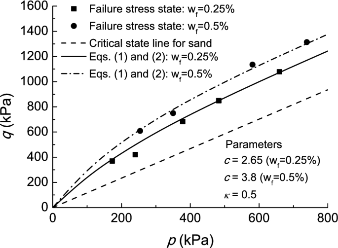

  

  Parameters $c$ and $\kappa$ for polypropylene-fiber-reinforced Hostun sand

• (b) $\mu$: Once $c$ and $\kappa$ are determined, a preliminary value for $\mu$ can be obtained by best fitting the $\varepsilon_{{\rm q}}-q$ relationship of FRS with $x = 0$. This is because the $\varepsilon_{{\rm q}}-q$ relationship is mainly affected by $\mu$ with fixed $c$ and $\kappa$, and the $\varepsilon_{{\rm q}}-\varepsilon_{{\rm v}}$ relationship is less sensitive to $\mu$ (Fig. 6).

  Fig. 6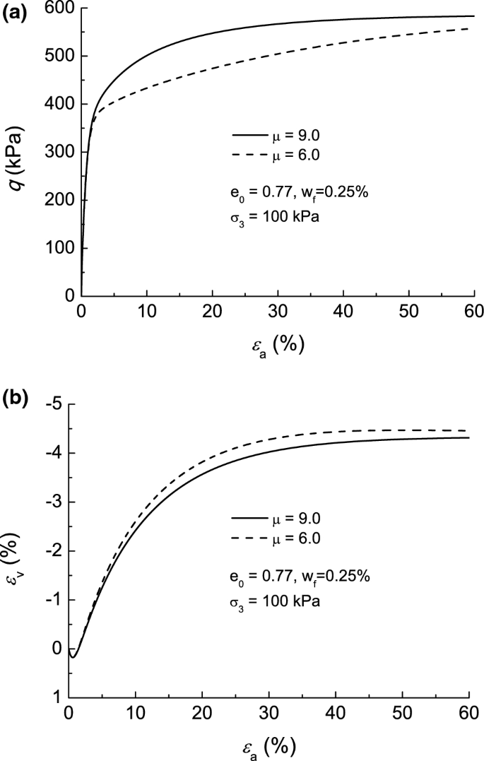

  

  Effect of the parameter $\mu$ on the simulated stress–strain relationship for FRS in a drained triaxial compression test: a the $\varepsilon_{{\rm a}}-q$ relationship, b the $\varepsilon_{{\rm a}}-\varepsilon_{{\rm v}}$ relationship

• (c) $x$: Finally, $x$ can be determined through best fitting the $\varepsilon_{{\rm q}} \left( {\varepsilon_{{\rm a}} } \right) - \varepsilon_{{\rm v}}$ relationship of FRS. Note that the preliminary $\mu$ may have to be tuned to get the best model simulations, as $x$ has influence on the $\varepsilon_{{\rm q}} \left( {\varepsilon_{{\rm a}} } \right) - q$ relationship as well (Fig. 3). Only a small adjustment to $\mu$ is need if $\left| x \right|$ is close to 1, which can be seen in the simulations shown in Fig. 3. It is recommended that two tests for FRS should be used for determining $\mu$ and $x$.

The test results for four fiber-reinforced sands are used in the model validation, including polypropylene-fiber-reinforced Hostun sand, polypropylene-fiber-reinforced Osorio sand [5, 33], a coarse, poorly graded sand (called JH sand to facilitate the discussion in this paper) reinforced by steel fibers [24, 27] and polypropylene-fiber-reinforced Hostun RF (S28) sand [7]. The model parameters for these sands are listed in Table 1. The test results which are used for the parameter determination will be given in the discussion on each soil below.

4.2 Polypropylene-fiber-reinforced Hostun sand

Several drained triaxial compression tests have been carried out on fiber-reinforced Hostun sand at the University of Glasgow. Hostun sand is a fine-grained and uniformly graded sand with sub-angular to angular particles. The mean particle diameter D₅₀ is 0.33 mm, and the uniformity coefficient C_u is 1.4. The specific gravity G_s is 2.64. The maximum and minimum void ratios, e_max and e_min, are 1.0 and 0.66, respectively [2]. Polypropylene fibers with a specific gravity G_f = 0.91 are used. The length $l$ and diameter of the fibers $D_{{\rm f}}$ are 35 mm and 0.088 mm, respectively. FRS with $w_{{\rm f}} = 0.25\%$ and $w_{{\rm f}} = 0.5\%$ was tested. Enlarged and lubricated end platens with a diameter of 50 mm were used. The sample diameter and height were 40 mm and 80 mm, respectively. The samples were prepared by moist tamping. Because of the magnitude of the strain reached, natural (true) strains $\varepsilon_{{\rm n}}$ calculated from the measured linear strains $\varepsilon_{{\rm l}}$ are used for both the axial strain $\varepsilon_{{\rm a}}$ and volumetric strain $\varepsilon_{{\rm v}}$.

The parameters $c$ and $\kappa$ are determined using all the test data (Fig. 5), while $\mu$ and $x$ are determined based on the test results with $\sigma_{3} = 300 {{\rm kPa}}$ (Fig. 7). Figures 7, 8 and 9 show the model predictions (curves) for the test data (dots) with $\sigma_{3}$ = 300 kPa, 200 kPa and 100 kPa, respectively. The parameter $x$ is found to be positive for this soil, indicating that the FRS ‘feels’ that its effective skeleton void ratio $e^{{\rm s}}$ is greater than $e$. This is because the FRS samples are prepared to have similar void ratio with that of pure sand. Generally, the model gives satisfactory prediction for the $\varepsilon_{{\rm a}} - q$ and $\varepsilon_{{\rm a}} - \varepsilon_{{\rm v}}$ relationships. But the strain softening toward the end of the tests with $w_{{\rm f}} = 0.25\%$ has not been captured. It is found that the sudden decrease in $q$ in these tests is caused by the development of clear shear bands in the samples. Were the deformation to have remained uniform in the sample, there would not be such sudden decrease in $q$. It is worth mentioning that in almost all fiber-reinforced sands such a strain softening response is not observed when $w_{{\rm f}} \ge 0.3\%$ [24]. It could thus be concluded that, to avoid localized soil failure, the optimum $w_{{\rm f}}$ for FRS should be at least 0.3% for practical applications [32].

Fig. 7

Model predictions for the stress–strain relationship of polypropylene-fiber-reinforced Hostun sand in drained triaxial compression tests with $\sigma_{3}$ = 300 kPa: a the $\varepsilon_{{\rm a}} - q$ relationship, b the $\varepsilon_{{\rm a}} - \varepsilon_{{\rm v}}$ relationship

Fig. 8

Model predictions for the stress–strain relationship of polypropylene-fiber-reinforced Hostun sand in drained triaxial compression tests with $\sigma_{3}$ = 200 kPa: a the $\varepsilon_{{\rm a}} - q$ relationship, b the $\varepsilon_{{\rm a}} - \varepsilon_{{\rm v}}$ relationship

Fig. 9

Model predictions for the stress–strain relationship of polypropylene-fiber-reinforced Hostun sand in drained triaxial compression tests with $\sigma_{3}$ = 100 kPa: a the $\varepsilon_{{\rm a}} - q$ relationship, b the $\varepsilon_{{\rm a}} - \varepsilon_{{\rm v}}$ relationship

4.3 Steel-fiber-reinforced JH sand

Drained triaxial compression tests on JH sand (D₅₀ = 0.89 mm, C_u = 1.52, G_s = 2.65, e_min = 0.56, e_max = 0.89) reinforced by steel fibers (G_f = 7.85, $D_{{\rm f}}$ = 0.64 mm, aspect ratio $a_{{\rm r}} = l /D_{{\rm f}}$ = 40) have been reported [24, 27]. The sample preparation method is discussed in [27]. All the samples have an initial void ratio $e_{0} = 0.66$. There are insufficient data for getting the location of the critical state line of JH sand in the $e - p$ plane, and therefore, $\lambda_{{\rm c}}$ and $\xi$ are estimated based on the parameters for Hostun sand, which are found to be very similar for various sands [13]. Since all the pure sand samples still show volumetric expansion toward the end of the test, the parameter $e_{\Gamma }$ is estimated to be close to the e_max of this sand, which is similar to the case for Hostun sand. The parameters of $c$ and $\kappa$ are determined based on the failure stress states reported in [24]. The rest of the model parameters are determined using the test results shown in Fig. 10 based on the procedure given at the beginning of this section.

Fig. 10

Comparison between the drained triaxial compression test results and model predictions for steel-fiber-reinforced JH sand with $w_{{\rm f}} = 6.0 \%$ and $a_{{\rm r}}$ = 40 (data from [27]): a the $\varepsilon_{{\rm a}} - q$ relationship, b the $\varepsilon_{{\rm a}} - \varepsilon_{{\rm v}}$ relationship

Comparison between the model predictions (curves) and test data (dots) is shown in Figs. 10 and 11. The predicted $\varepsilon_{{\rm a}} - q$ relationships are in excellent agreement with the test data. Satisfactory prediction for the $\varepsilon_{{\rm a}} - \varepsilon_{{\rm v}}$ relationships is also achieved, with the model mainly overestimating the volumetric expansion for the test with $\sigma_{3}$ = 400 kPa and $w_{{\rm f}}$ = 2.0% (Fig. 11).

Fig. 11

Comparison between the drained triaxial compression test results and model predictions for steel-fiber-reinforced JH sand with $w_{{\rm f}}$ = 2.0% and $a_{{\rm r}}$ = 40 (data from [24]): a the $\varepsilon_{{\rm a}} - q$ relationship, b the $\varepsilon_{{\rm a}} - \varepsilon_{{\rm v}}$ relationship

4.4 Polypropylene-reinforced Osorio sand

A series of drained triaxial compression tests on Osorio sand (D₅₀ = 0.16 mm, C_u = 2.1, G_s = 2.62, e_min = 0.6, e_max = 0.9) reinforced by polypropylene fibers (G_f = 0.91, $D_{{\rm f}}$ = 0.023 mm, $l$ = 24 mm) have been reported [5, 33]. The samples were prepared by moist tamping. The parameters $c$ and $\kappa$ are obtained based on the failure points [5, 33]. The test data in Fig. 12 are used to determine all the remaining parameters. Two drained triaxial tests with different stress paths are shown in Fig. 13, one with constant $\sigma_{3}$ (= 20 kPa) and the other with ${{\rm d}}q = - 3{{\rm d}}p$ and initial confining pressure $\sigma_{3i}$ of 200 kPa [5]. In contrast to the previous two sands, this sand has a negative $x$, which is similar to the tests reported in [9].

Fig. 12

Model predictions for the stress–strain relationship of polypropylene-fiber-reinforced Osorio sand in drained triaxial compression tests with $\sigma_{3}$ = 100 kPa (data from [33]): a the $\varepsilon_{{\rm a}} - q$ relationship, b the $\varepsilon_{{\rm a}} - \varepsilon_{{\rm v}}$ relationship

Fig. 13

Model predictions for the stress–strain relationship of polypropylene-fiber-reinforced Osorio sand in drained triaxial compression tests with different stress paths (data from [5]): a the $\varepsilon_{{\rm a}} - q$ relationship, b the $\varepsilon_{{\rm a}} - \varepsilon_{{\rm v}}$ relationship

The model prediction is in good agreement with the test data in Fig. 12. But it is evident that there is obvious discrepancy between the test data and model prediction on soil dilatancy in Fig. 13b. This could be because the model itself needs to be improved to get better predictions, such as the evolution of $p_{{\rm f}}$ and expression for $e^{{\rm s}}$. Meanwhile, it is noticed that the tests in Figs. 12 and 13 were done by different researchers. Though they followed the same test procedure, their samples might have slightly different internal structure which had influence on the mechanical behavior. Indeed, it is found by Ibraim et al. [18] that the internal structure of FRS, particularly the distribution of fibers, has profound effect on the soil dilatancy ($\varepsilon_{{\rm a}} - \varepsilon_{{\rm v}}$ relationship). Therefore, better model predictions could be achieved by accounting for the effect of fiber distribution in FRS [23, 28, 34].

4.5 Polypropylene-reinforced Hostun RF (S28) sand

Both drained and undrained triaxial compression tests on Hostun RF (S28) sand (D₅₀ = 0.38 mm, C_u = 1.9, G_s = 2.65, e_min = 0.648, e_max = 1.041) reinforced by Loksand™ fibers (G_f = 0.91, $D_{{\rm f}}$ = 0.1 mm, $l$ = 35 mm) have been reported in [7]. The parameters for pure sand are determined using all the test results on sand (Figs. 14, 15, 16, 17 and 18). The fiber-reinforced samples are found to show strain hardening even at the end of the test with large axial strain level and no failure is observed, making it difficult to get $c$ and $\kappa$ for this soil from the test data directly. Therefore, an alternative method has been used in determining the model parameters associated with fibers. $\kappa = 1.0$ is assumed first. Compared to the other three FRS samples, the maximum fiber reinforcement for this FRS is expected to be reached at a much higher axial strain level ($\varepsilon_{{\rm a}} > 40\%$), a smaller $\mu \left( { = 6.0} \right)$ is assumed. Because smaller $\mu$ makes the evolution rate of $p_{{\rm f}}$ lower and the maximum fiber reinforcement to be reached at a higher shear strain level. $c$ is then determined by best fitting the $\varepsilon_{{\rm a}} - q$ relationship in Figs. 14 (drained tests) and 17 (undrained triaxial compression tests). Finally, $x$ is determined based on the $\varepsilon_{{\rm a}} - \varepsilon_{{\rm v}}$ relationship in Fig. 14.

Fig. 14

Comparison between model prediction and test data on polypropylene-fiber-reinforced Hostun RF (S28) sand (loose sand) in drained triaxial compression (data from [7]): a the $\varepsilon_{{\rm a}} - q$ relationship, b the $\varepsilon_{{\rm a}} - \varepsilon_{{\rm v}}$ relationship

Fig. 15

Comparison between model prediction and test data on polypropylene-fiber-reinforced Hostun RF (S28) sand (medium dense sand) in drained triaxial compression (data from [7]): a the $\varepsilon_{{\rm a}} - q$ relationship, b the $\varepsilon_{{\rm a}} - \varepsilon_{{\rm v}}$ relationship

Fig. 16

Comparison between model prediction and test data on polypropylene-fiber-reinforced Hostun RF (S28) sand (dense sand) in drained triaxial compression (data from [7]): a the $\varepsilon_{{\rm a}} - q$ relationship, b the $\varepsilon_{{\rm a}} - \varepsilon_{{\rm v}}$ relationship

Fig. 17

Comparison between model prediction and test data on polypropylene-fiber-reinforced Hostun RF (S28) sand in undrained triaxial compression with $\sigma_{3}$ = 200 kPa (data from [17]): a the $\varepsilon_{{\rm a}} - q$ relationship, b the effective stress path

Fig. 18

Comparison between model prediction and test data on polypropylene-fiber-reinforced Hostun RF (S28) sand in undrained triaxial compression with $\sigma_{3}$ = 100 kPa (data from [17]): a the $\varepsilon_{{\rm a}} - q$ relationship, b the effective stress path

The model predictions (curves) for the tests (dots) are shown in Figs. 14, 15, 16, 17 and 18, which include tests with different initial void ration and confining pressure. In general, the model prediction gives reasonable prediction of the soil response, but it can be further improved in the following aspects. First, the model does not give a good prediction for the bilinear shape of the $\varepsilon_{{\rm a}} - q$ relationship in drained tests on loose and medium dense samples (Figs. 14 and 15). For the dense sand case (Fig. 16), the predicted $\varepsilon_{{\rm a}} - q$ relationship is in better agreement with the test results, as its shape is not bilinear but closer to that for the other fiber-reinforced sands. This could be due to that the development of fiber reinforcement, which is described by the evolution of $p_{{\rm f}}$ of the model [Eq. (6)], does not work very well for the tests in Figs. 14 and 15. Improved model predictions can be achieved by using a different evolution law for $p_{{\rm f}}$. Secondly, the model does not capture the $\varepsilon_{{\rm a}} - \varepsilon_{{\rm v}}$ relationship well in Fig. 16. This is partly due to that the model prediction for pure sand is not satisfactory, as the parameters for pure sand are obtained to get the optimum prediction for all the tests rather than a single one.

In proposing a better formulation for the evolution of $p_{{\rm f}}$, it is crucial to consider the effect of induced anisotropy (or increased anisotropy in fiber orientation), particularly when the fiber content is relatively large [26]. This is because of the substantial rotation of the fibers at large strain, which makes the fibers less and less inclined to the horizontal direction. The induced anisotropy can cause an inflection point in the measured $\varepsilon_{{\rm a}} - \varepsilon_{{\rm v}}$ curve (Figs. 14, 15). Detailed discussion on this issue can be found in Michalowski and Čermák [26].

5 Conclusion

A new method for constitutive modeling of FRS is developed. It is based on the assumption that the strain of FRS is dependent on the deformation of the sand skeleton, while the effective skeleton stress and effective skeleton void ratio, which should be used in modeling the dilatancy relation, plastic hardening and elastic stress–strain relationship of FRS, are affected by fiber inclusion. The effective skeleton stress evolves with the shear strain, and the effective skeleton void ratio is dependent on the fiber content and sample preparation method.

A critical state model for FRS in the triaxial stress space is proposed using the concept of effective skeleton stress and void ratio. Four new parameters are introduced to characterize the fiber inclusion on the mechanical behavior of sand. All of them can be easily determined based on the triaxial test data on FRS, without measuring the stress–strain relationship of individual fibers. The model has been used to predict the stress–strain relationship of four fiber-reinforced sands (35 tests in total) in triaxial compression tests under different stress paths. Satisfactory agreement between the test data and model prediction has been observed.

The major objective of this work is to study how to model the mechanical behavior of FRS using the concept of effective skeleton stress and void ratio, rather than to develop a fully fledged constitutive model. Future work will be done to make more improvements to the constitutive model:

• (a) The parameter $c$ has to be specified for FRS with different fiber contents. Micromechanical analysis can be done to give a general expression for $c$, which can account for the property of fibers and sand [26, 27].

• (b) The evolution law for $p_{{\rm f}}$ needs to be improved for some FRS (e.g., the fiber-reinforced Hostun RF (S28) sand in this study) through considering the induced anisotropy associated with fiber rotation [26].

• (c) It is important to realize that the fiber orientation in FRS is highly anisotropic, which makes the mechanical behavior of FRS dependent on the loading (or strain increment) direction [24,25,26]. Such effect is not accounted for in the present model. But the model can be readily extended to account for multi-axial loading and fiber orientation anisotropy [11].

References

Ahmad F, Bateni F, Azmi M (2010) Performance evaluation of silty sand reinforced with fibres. Geotext Geomembr 28(1):93–99
Azeiteiro RJ, Coelho PA, Taborda DM, Grazina JC (2017) Critical state-based interpretation of the monotonic behaviour of Hostun Sand. J Geotech Geoenviron Eng 143(5):04017004
Babu GS, Vasudevan AK, Haldar S (2008) Numerical simulation of fiber-reinforced sand behavior. Geotext Geomem 26(2):181–188
Been K, Jefferies MG (1985) A state parameter for sands. Géotechnique 35(2):99–112
Consoli NC, Heineck KS, Casagrande MDT, Coop MR (2007) Shear strength behavior of fiber-reinforced sand considering triaxial tests under distinct stress paths. J Geotech Geoenviron Eng 133(11):1466–1469
di Prisco C, Nova R (1993) A constitutive model for soil reinforced by continuous threads. Geotext Geomembr 12(2):161–178
Diambra A (2010) Fibre reinforced sands: experiments and constitutive modelling. Ph.D. thesis, University of Bristol
Diambra A, Ibraim E, Muir Wood D, Russell AR (2010) Fibre reinforced sands: experiments and modelling. Geotext Geomembr 28(3):238–250
Diambra A, Ibraim E, Russell AR, Wood DM (2013) Fibre reinforced sands: from experiments to modelling and beyond. Int J Numer Anal Methods Geomech 37(15):2427–2455
Ding D, Hargrove S (2006) Nonlinear stress-strain relationship of soil reinforced with flexible geofibers. J Geotech Geoenviron Eng 132(6):791–794
Gao ZW, Diambra A (2020) A multiaxial constitutive model for fibre-reinforced sand. Geotechnique. https://doi.org/10.1680/jgeot.19.P.250
Gao ZW, Zhao JD (2013) Evaluation on failure of fibre-reinforced sand. J Geotech Geoenviron Eng 139(1):95–106
Gao ZW, Zhao JD, Li XS, Dafalias YF (2014) A critical state sand plasticity model accounting for fabric evolution. Int J Numer Anal Methods Geomech 38(4):370–390
Gao ZW, Hong Y, Wang L (2020) Constitutive modelling of fine-grained gassy soil: a composite approach. Int J Numer Anal Methods Geomech. https://doi.org/10.1002/nag.3065
Hong Y, Wang L, Zhang J, Gao Z (2019) 3D elastoplastic model for fine–grained gassy soil considering the gas–dependent yield surface shape and stress–dilatancy. J Eng Mech 146(5):04020037
Ibraim E, Maeda K (2007) Numerical analysis of fibre-reinforced granular soils. In: Otani J, Miyata Y, Mukunoki T (eds) New horizons in earth reinforcement, Proceedings of 5th international symposium on earth reinforcement, IS Kyushu’07. Balkema, Rotterdam, pp 387–393
Ibraim E, Diambra A, Muir Wood D, Russell AR (2010) Static liquefaction of fibre reinforced sand under monotonic loading. Geotext Geomembr 28(4):374–385
Ibraim E, Diambra A, Russell AR, Muir Wood D (2012) Assessment of laboratory sample preparation for fibre reinforced sands. Geotext Geomembr 34:69–79
Kong Y, Zhou A, Shen F, Yao Y (2019) Stress–dilatancy relationship for fiber-reinforced sand and its modeling. Acta Geotech 14:1871–1881
Li XS, Dafalias YF (2000) Dilatancy for cohesionless soils. Géotechnique 50(4):449–460
Li XS, Dafalias YF (2002) Constitutive modeling of inherently anisotropic sand behavior. J Geotech Geoenviron Eng 128(10):868–880
Li XS, Wang Y (1998) Linear representation of steady-state line for sand. J Geotech Geoenviron Engng 124(12):1215–1217
Mandolini A, Diambra A, Ibraim E (2019) Strength anisotropy of fibre-reinforced sands under multiaxial loading. Géotechnique 69(3):203–216
Michalowski RL (1996) Micromechanics-based failure model of granular/particulate medium with reinforcing fibers. Technical Report, Air Force office of Scientific Research, USA
Michalowski RL (2008) Limit analysis with anisotropic fiber-reinforced soil. Geotechnique 58(6):489–501
Michalowski RL, Čermák J (2002) Strength anisotropy of fiber-reinforced sand. Comput Geotech 29(4):279–299
Michalowski RL, Zhao A (1996) Failure of fiber-reinforced granular soils. J Geotech Eng 122(3):226–234
Muir Wood D, Diambra A, Ibraim E (2016) Fibres and soils: a route towards modelling of root–soil systems. Soils Found 56(5):765–778
Richart FE, Hall JR Jr, Woods RD (1970) Vibrations of soils and foundations. Prentice-Hall, Englewood Cliffs
Santoni RL, Webster SL (2001) Airfields and road construction using fiber stabilization of sands. J Transp Eng 127(2):96–104
Senetakis K, Li H (2017) Influence of stress anisotropy on small-strain stiffness of reinforced sand with polypropylene fibres. Soils Found 57(6):1076–1082
Shukla SK (2017) Fundamentals of fibre-reinforced soil engineering. Springer, Singapore
Silva Dos Santos AP, Consoli NC, Baudet BA (2010) The mechanics of fibre-reinforced sand. Géotechnique 61(10):791–799
Soriano I, Ibraim E, Andò E, Diambra A, Laurencin T, Moro P, Viggiani G (2017) 3D fibre architecture of fibre-reinforced sand. Granul Matter 19(4):75
Wu TH, Mckinnel WP III, Swanston DN (1979) Strength of tree roots and landslides on Prince of Wales Island, Alaska. Can Geotech J 16(1):19–33
Zornberg J (2002) Discrete framework for equilibrium analysis of fibre reinforced soil. Géotechnique 52(8):593–604
Acknowledgements
The authors would like to acknowledge Dr. Andrea Diambra at University of Bristol for sharing his data on fiber-reinforced Hostun RF (S28) sand. The authors also would like to acknowledge the contribution of Dr. Thomas Shire at University of Glasgow, who helped to improve the writing of the paper.
Author information
Authors and Affiliations
Corresponding author
Additional information
Publisher's Note
Springer Nature remains neutral with regard to jurisdictional claims in published maps and institutional affiliations.
Rights and permissions
Open Access This article is licensed under a Creative Commons Attribution 4.0 International License, which permits use, sharing, adaptation, distribution and reproduction in any medium or format, as long as you give appropriate credit to the original author(s) and the source, provide a link to the Creative Commons licence, and indicate if changes were made. The images or other third party material in this article are included in the article's Creative Commons licence, unless indicated otherwise in a credit line to the material. If material is not included in the article's Creative Commons licence and your intended use is not permitted by statutory regulation or exceeds the permitted use, you will need to obtain permission directly from the copyright holder. To view a copy of this licence, visit http://creativecommons.org/licenses/by/4.0/.
About this article
Cite this article
Gao, Z., Lu, D. & Huang, M. Effective skeleton stress and void ratio for constitutive modeling of fiber-reinforced sand. Acta Geotech. 15, 2797–2811 (2020). https://doi.org/10.1007/s11440-020-00986-w
Received:
Accepted:
Published:
Issue Date:
DOI: https://doi.org/10.1007/s11440-020-00986-w