
Abstract
For complex scalar waves, a convenient measure of the local oscillations and ('faster than Fourier') superoscillations is the phase gradient vector: the local wavevector, or weak value of the momentum operator. This vanishes for standing waves, described by real functions ψ(r); for such waves, an alternative descriptor of oscillations is the local weak value of the square of one of the momentum components, i.e.  , here called the 'weak curvature'. Superoscillations correspond to places where K2 lies outside the interval 0 ⩽ K2 ⩽ 1. Two illustrations are given. First is an explicit family of real waves in dimension d = 2, with arbitrarily strong superoscillations; this could represent Neumann standing modes in a strip waveguide. Second is an exact calculation of the probability distribution of K2 for Gaussian random real waves in d dimensions. This decays as
  , as a consequence of the codimension 1 of nodes (e.g. nodal lines for d = 2). The superoscillation probability varies from 0.3918 (d = 2) to 0.3041 (d = ∞).
Export citation and abstract BibTeX RIS

Content from this work may be used under the terms of the Creative Commons Attribution 4.0 licence. Any further distribution of this work must maintain attribution to the author(s) and the title of the work, journal citation and DOI.
1. Introduction
A distinctive feature of waves is their pattern of oscillations, in particular the rate at which wavefunctions vary. For monochromatic waves, the smallest scale was conventionally regarded as determined by the wavelength. But it is now recognised that although such waves are bandlimited, they can vary locally on sub-wavelength scales: arbitrarily faster than their fastest Fourier component—they can superoscillate [1]. In its modern form, the subject originated in quantum measurement theory [2, 3], but has expanded into many areas, for example mathematics [4, 5], signal and image processing [6–11], and optics [12–14]. The underlying 'faster than Fourier' idea was anticipated in radar theory [15], optics [16–18], and the fine structure near wave singularities [19, 20].
In previous work, superoscillations were described as fast variations of the local phase.This applies to waves that can be represented as complex functions of position. It is not immediately obvious how to describe superoscillations for the real wavefunctions that represent standing waves. My aim here is to explore one such way. First, I explain the problem in more detail.
For complex scalar functions ψ(
r) of position
r
= (x1, x2, ...xd
) in d dimensions, there is a natural and familiar way to describe the oscillations: by the gradient of phase, i.e. the local wavevector
k
(
r
). This can be defined in several alternative ways in terms of the momentum operator  [21]:
[21]:
In particular, the second equality represents
k
(
r
) as the 'weak value' of  in the preselected state ψ, with position
r
postselected. This term originated in quantum measurement theory [2, 3], but is convenient here because it is applicable to fast-varying complex functions of all kinds,in particular waves.
in the preselected state ψ, with position
r
postselected. This term originated in quantum measurement theory [2, 3], but is convenient here because it is applicable to fast-varying complex functions of all kinds,in particular waves.
For monochromatic waves, ψ( r ) is a band-limited function, expressible as a superposition of plane waves, all with the same wavenumber k0, travelling in different directions. For some positions r , the length | k ( r )| exceeds k0: this corresponds to the superoscillations [1, 4, 5]. As is clear from the denominators in (1.1), superoscillations are concentrated near the zeros of ψ, i.e. the nodes—points in 2D, lines in 3D, alternatively described as phase singularities, wave vortices or wave dislocations [19, 20, 22, 23].
This convenient picture fails for the real waves to be studied here, because, according to the definition (1.1), k ( r ) vanishes. An easy fix is available for travelling time-dependent real waves that can be written in the form

At each point, such waves oscillate sinusoidally, with the phase of the oscillations depending on position; the complex function ψ is the 'analytic signal' [24] representing the real wave Ψ. For this case, k ( r ) as defined in (1.1) can be reconstructed by measuring the real wave atany two times in quadrature:

But this fails for standing waves, for example cavity modes and quantum eigenfunctions of systems with time-reversal symmetry. Then ψ is real and the oscillations of the real function Ψ are in phase simultaneously everywhere:

In the plane-wave superposition representing ψ, each component wavevector k n is accompanied by its opposite − k n , so k ( r ) = 0. This is the case to be studied here, for real waves satisfying

in which for convenience the monochromatic wavenumber is chosen as k0 = 1 (i.e. the wavelength is λ = 2π). How can the oscillations of ψ( r ) be conveniently represented? One possibility is create a complex function from the real ψ by choosing (by analogy with the analytic signal) one of each pair ± k n ; but the ambiguity in the choice makes the resulting complexfunction, and the associated local wavevector k ( r ), non-unique, so this strategy fails.
Although the weak value of  vanishes for real ψ, the weak value of the square of the momentum,

does not. But the solutions of (1.5) are eigenstates of  and its weak value is trivially unity everywhere, so it gives no interesting information about the wave's oscillations. But this isnot true for the squares of individual momentum components, e.g. the x component. Therefore I propose describing the local oscillations of real standing waves by the weak value

I call this the weak curvature. Of course the y (or any other) derivative could equally be chosen, but for the important case d = 2 this gives no further information because thecorresponding weak curvature is 1—the curvature defined by the x derivative. In principle, the weak curvature could be obtained from measurements of the intensity (energy density)  , using

The eigenstates of  are individual plane waves exp(ikx
x), in which for solutions of (1.5) the spectrum of
are individual plane waves exp(ikx
x), in which for solutions of (1.5) the spectrum of  is
is  ; positions where K2(
r
) is outside this interval correspond to superoscillations. It is clear that, as with the wavevectors
k
(
r
) for complex waves, the superoscillations are concentrated near the nodes. For these real waves, the nodes arecodimension 1 singularities of K2, i.e. lines for d = 2 and surfaces for d = 3. We anticipate that these nodes will have a stronger effect on the superoscillations, i.e. on K2, than the effect on
k
(
r
) of the zeros of complex scalar waves, which are codimension 2 singularities: points for d = 2 and lines for d = 3. (The opposite case, discussed recently [25], is complex vector waves, such as the electric field
E
or the magnetic field
B
representing generally polarised travelling optical fields. Then, the singularities of the suitably defined wavevectors are codimension 6, so the superoscillations are much weaker; and for the six-vector (
E
,
B
) the singularities are codimension 12, so the superoscillations are weaker still.)
; positions where K2(
r
) is outside this interval correspond to superoscillations. It is clear that, as with the wavevectors
k
(
r
) for complex waves, the superoscillations are concentrated near the nodes. For these real waves, the nodes arecodimension 1 singularities of K2, i.e. lines for d = 2 and surfaces for d = 3. We anticipate that these nodes will have a stronger effect on the superoscillations, i.e. on K2, than the effect on
k
(
r
) of the zeros of complex scalar waves, which are codimension 2 singularities: points for d = 2 and lines for d = 3. (The opposite case, discussed recently [25], is complex vector waves, such as the electric field
E
or the magnetic field
B
representing generally polarised travelling optical fields. Then, the singularities of the suitably defined wavevectors are codimension 6, so the superoscillations are much weaker; and for the six-vector (
E
,
B
) the singularities are codimension 12, so the superoscillations are weaker still.)
In section 2 we construct explicit families of real waves for d = 2, possessing tunable superoscillations of arbitrary strength. Contrasting this are the superoscillations that occur naturally in random real waves. These are discussed in section 3 for arbitrary dimension d. The probability distribution of K2, and in particular the superoscillation probability, that is, the probability that K2 lies outside the interval 0 ⩽ K2 ⩽ 1, is calculated by following the pioneering calculation for random complex waves for d = 2 [26], and its generalisation [27] for arbitrary d.At the end of section 3 is a brief discussion of possible superoscillations for evanescent waves.
2. Superoscillatory real waveguide modes
The construction of superoscillatory waves ψ( r ) in the plane r = (x, y) starts with the x axis, where we define the wave in terms of the canonical and well-understood superoscillatory function [2, 4, 28]:
This is band-limited, with wavevectors 1 ⩽ km ⩽ 1; we consider a > 1, and N ⩾ 1 an even integer. The function ψ(x, 0) is periodic, with period Nπ. Near x = 0 (mod(Nπ), ψ(x, 0)is superoscillatory, with the parameter a representing the degree of superoscillation:

Thus the parameter N controls the interval over which ψ(x,0) superoscillates. Figure 1(a) illustrates the function ψ(x, 0), plotted logarithmically to indicate the large range, andfor comparison 1 + log10 |cos x|, which oscillates according to the highest Fourier component.

Figure 1. Superoscillatory wave (2.1) on the x axis, for a = 6, N = 8. (a) Full red curve: the function (2.1), dashed curve: 1 + log10 |cos x|. (b) The corresponding weak curvature K2(x, 0).
Download figure:
Standard image High-resolution imageThe weak curvature K2(x, 0), illustrated in figure 1(b), shows the expected divergences at the nodes of ψ. At x = 0, the value is

This is outside the spectral range, reflecting the superoscillatory behaviour of ψ at the origin.
To extend ψ(x, 0) away from the x axis to solutions ψ(x, y) of (1.5), we introduce y components

for each of the Fourier components in (2.3). There are different possibilities, depending on the choice of signs; three natural choices are

All are x periodic and could represent superoscillatory standing-wave modes of a strip waveguide −Nπ/2 ⩽ x⩽ Nπ/2, −∞ < y < +∞. ψ1(x, y) has Neumann boundary conditions at the edges; all three could alternatively represent modes on the surface of a cylinder.
Figure 2 shows the nodal domains of the three modes. In (a) and (d), the small separation of nodal lines near the origin indicates the superoscillatory nature of the wave ψ1, in whichthe component waves are separable in x and y, For ψ2 and ψ3, whose components are not separable, the superoscillations are invisible in (b) and (c), and revealed only under high y magnification in (e) and (f), as rapid undulations of the nodal lines.

Figure 2. Nodal domains of strip waveguide standing modes (2.5), for a = 6, N = 8. (a–d): ψ1; (b–e): ψ2; (c–f): ψ3. In (a–c) the region shown is a square of side Nπ, i.e. one period in x. In (d–f) the x interval shown is one 'wavelength' period 2π, corresponding to the highest Fourier component, and in (e, f) the y magnifications show the superoscillatory variation of the nodal lines.
Download figure:
Standard image High-resolution image3. Random real superoscillations
We can understand the typical oscillations of real functions ψ(
r
) by calculating the probability distribution of the weak curvature K2 for an ensemble of solutions of (1.5). From thedefinition (1.7), and with  denoting ensemble averages, this is

Here  is the joint probability distribution of ψ and
  ; these quantities are correlated because (1.5) implies that
  is usually negative/positive where ψ is positive/negative.
We can easily find the large |K2| behaviour of the distribution without detailed calculation, using two facts: large K2 comes from the neighbourhood of the nodes, and nodes are hypersurfaces of codimension 1 (lines for d = 2, surfaces for d = 3, etc). Symbolically, againusing (1.7),

For a more precise calculation, we give the details for d = 2 and then state the generalisation to arbitrary d. It is necessary to define the ensemble. The natural choice is an isotropic random superposition of real plane waves with random phases and wavevector directions:

From the central limit theorem, the statistics of ψ and its derivatives are Gaussian.
Figure 3 shows a sample wave. Figure 4 illustrates the associated weak curvature. It is clear from figure 4(a) that the weak curvature on the x axis is dominated by the intersections of the nodal lines with the axis. Crossings of nodal lines would be stronger singularities but do not occur generically (they have codimension 3); avoided crossings do occur, and figure 4(b) illustrates the weak curvature near one of them (in the square in figure 3(b)).
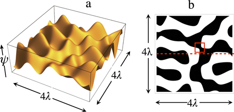
Figure 3. A sample real wave ψ(x,y) from the ensemble (3.3), displayed as (a) the height ψ of a surface, (b) signψ, showing the nodal lines. In (b) the red dashed line and the box refer to figure 4.
Download figure:
Standard image High-resolution image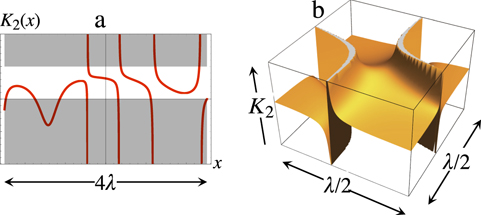
Figure 4. Weak curvature for the wave shown in figure 3(a) along the x axis (red dashed line in figure 3(b), with the superoscillatory region (K2 < 0, K2 > 1) shaded; (b) near the avoided crossing of two nodal lines (red box in figure 3(b)).
Download figure:
Standard image High-resolution imageTo find  , we need the following averages, which are simple consequences of (3.1):

These averages determine the required joint distribution:

The integrals in (3.1) are elementary when evaluated in the order ψ'', t, ψ, leading to the weak curvature distribution

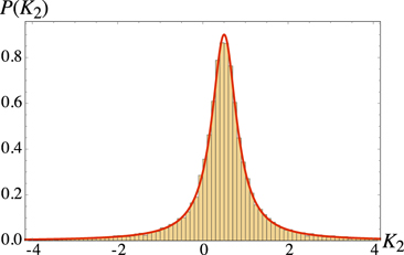
This is a Cauchy (Lorentzian) distribution. Figure 5 shows its graph, together with a histogram calculated numerically from the ensemble (3.3).
Figure 5. Weak curvature distribution (3.6) for d = 2 (red curve), compared with a simulation using 20 000 sample waves from the ensemble (3.3), each with N = 20 plane waves (histogram).
Download figure:
Standard image High-resolution image
For large K2, P(K2) has the inverse-square asymptotics (3.2) anticipated from thecodimension argument. The superoscillation probability, that the weak curvature at a random position in a wave from the ensemble lies outside the spectrum of the operator  is,
is,

This is larger than the superoscillation probability 1/3 for complex Gaussian random waves in the plane [26], because the dominating singularities for real waves—nodal lines—have smaller codimension than the wave vortex singularities for complex waves.
Generalisation to arbitrary dimension d is straightforward. The ensemble consists of superpositions of the form (3.3), but where the wavevectors k n are real vectors whose directions are randomly distributed on the surface of the unit sphere in d dimensions. The necessary Gaussian statistics are

The first equality is a definition, the second follows from isotropy, and the third is calculated using hyperspherical polar coordinates for the wavevectors k on the unit sphere in d dimensions. Instead of (3.6) the weak curvature distribution is

Thus the Cauchy distribution—again with the anticipated inverse-square decay—emerges as a universal scaling function for the weak curvature probability. The constants A and B vanish as d → ∞, so for high-dimensional waves the distribution condenses onto a δ-function at K2 = 0. The constants A and B also vanish for d = 1; this is because monochromatic waves in one dimension are sinusoids, for which K2 = 1 everywhere, so the distribution is a δ-function at K2 = 1. (For real Gaussian random functions of a single variable that are not monochromatic (i.e. which do not satisfy (1.5)), the distribution P(K2) also the Cauchy form (3.9).)
The superoscillation probability for arbitrary d, generalising (3.7), is

The first few values, and the large d limiting value, are

The value Psuper(1) = 0.5 can be understood as the monochromatic limit of a non-monochromatic band-limited real Gaussian random function of a single variable, as was discussed for complex waves in section 3 of [27].
A referee has suggested studying superoscillations for evanescent waves [29]. The simplest model real solution of (1.5) is the counterpart of the superposition (3.3) for d = 2:

Such waves are anisotropic: they oscillate in x but not y. The x oscillations are sub-wavelength (remember that the free-space wavenumber is k0 = 1), but these are not superoscillations per se, because the fast oscillations with wavenumbers q in the interval  are contained in the band-limited spectrum in (3.12). But it is possible that for particular y (e.g. y = 0) the sum is a superoscillatory function of x, so there would be 'sub-sub-wavelength' variations, with effective wavenumbers greater than
  . For this case, P(K2) would still have the universal Cauchy form.
4. Concluding remarks
The analysis presented here has explored the weak curvature K2 (equation (1.7)) as a quantitative measure of the effect of nodes on the local fluctuations of real monochromatic scalar waves. K2 is singular on the nodes, whose codimension implies a characteristic inverse-square decay in its probability distribution. As with other superoscillations, the dominance by the neighbourhood of nodes reflects the almost-perfect destructive interference of the plane-wave Fourier components in the superpositions (in this case real) constituting the waves.
Extensions can be envisaged.
- The superoscillatory strip/cylinder waveguide modes of section 2 could be modified to describe three-dimensional real modes in waveguides with rectangular cross section.
- The Gaussian random waves of section 3 could be made anisotropic by using a superposition with a direction-dependent distribution of wavevectors; the relatively large value 0.5 for d = 1 in (3.11) suggests that anisotropy might increase Psuper(d) for d > 1.
- The recent study of wavevectors in random complex vector waves [25] could be adapted for real waves; vector waves typically have no nodes, so the tail of P(K2) would decay faster.
More generally, the effect of nodes on statistics is a new example in the class of phenomena involving power-law tails dependent on the codimension of singularities (and distinct from the power-laws associated with fractals). Previous examples of such 'singularity-dominated strong fluctuations' include twinkling starlight [30, 31], crystal densities of states (van Hove singularities) [32], energy-level statistics involving bifurcations [33], negative moments of spectral determinants and zeta functions [34, 35], and the chaotically advected 'odour plume' that leads a male moth to his mate [36].
Acknowledgments
I thank Professor John Hannay for helpful conversations, and Professor Pragya Shukla and two referees for several suggestions.