Laurent series expansions of multiple zeta-functions of Euler–Zagier type at integer points

Abstract

We give explicit expressions (or at least an algorithm to obtain such expressions) of the coefficients of the Laurent series expansions of the Euler–Zagier multiple zeta-functions at any integer points. The main tools are the Mellin–Barnes integral formula and the harmonic product formulas. The Mellin–Barnes integral formula is used in the induction process on the number of variables, and the harmonic product formula is used to show that the Laurent series expansion outside the domain of convergence can be obtained from that inside the domain of convergence.

Appendix

The second-named author [11] studied limit values of $\zeta _r({\mathbf {s}})$ at the points ${\mathbf {m}}\in ({\mathbb {Z}}_{\le 0})^r$, and he gave a result on the limit values. In this appendix we give an alternative proof of his result by using the method of the present paper. To state the result of [11], we prepare some symbols and functions. For ${\mathbf {m}}\in {\mathbb {Z}}^r$ and ${\mathbf {s}}\in {\mathbb {C}}^r$, we put $\varepsilon _1=s_1-m_1,\ldots ,\varepsilon _r=s_r-m_r$ and $\varepsilon =\max \{|\varepsilon _1|,\ldots ,|\varepsilon _r|\}$. We also define

$$\begin{aligned} R_j({\mathbf {s}}):=\frac{s_j+\cdots +s_r-m_j-\cdots -m_r}{s_{j-1}+\cdots +s_r-m_{j-1}-\cdots -m_r} \end{aligned}$$

for $2\le j\le r$. When the denominator of $R_j(s)$ is 0 (that is the case $\varepsilon _1+\cdots +\varepsilon _r=0$), ${\mathbf {s}}$ is located on a singular locus in most cases. In what follows, we exclude such situation from our consideration.

Theorem

[11, Theorem 2] Let ${\mathbf {m}}\in ({\mathbb {Z}}_{\le 0})^r$ and ${\mathbf {s}}\in {\mathbb {C}}^r$. When all $R_j({\mathbf {s}})$ have limit values as $\varepsilon \rightarrow 0$, $\zeta _r({\mathbf {s}})$ converges to the value which is represented by the limit values of $R_j({\mathbf {s}})$ and the Bernoulli numbers, that is, we have

$$\begin{aligned} \zeta _r({\mathbf {s}})=\sum _{0\le h\le r-1}\sum _{2\le j_1<j_2<\cdots <j_h\le r} \left( C_{j_1j_2\cdots j_h}+O(\varepsilon )\right) R_{j_1}({\mathbf {s}})R_{j_2}({\mathbf {s}})\cdots R_{j_h}({\mathbf {s}}) \end{aligned}$$

(5.10)

where the constants $C_{j_1j_2\cdots j_h}$ are given by the Bernoulli numbers.

Remark

In the above theorem, when $h=0$, we define $(j_1,j_2,\ldots ,j_h)$ as empty set $\phi$, and we understand $R_{\phi }({\mathbf {s}})=1$.

Note that the constants $C_{j_1j_2\cdots j_h}$ are given explicitly in [11, Theorem 2] and depend on ${\mathbf {m}}$.

Here we reconsider this theorem from the viewpoint of our method. From Theorem 1.5, we can also give the limit value of $\zeta _r({\mathbf {s}})$ at ${\mathbf {m}}\in ({\mathbb {Z}}_{\le 0})^r$, but this limit value contains some integrals, so this limit value is more complicated than (5.10). Corollary 5.2 gives limit values with easy expressions. However this corollary holds only for $r=2$.

If we add the same condition as the above theorem, that is, if all $R_j({\mathbf {s}})$ have limit values as $\varepsilon \rightarrow 0$, we can also prove the above theorem from our method by induction. Hereafter we prove it.

Remark

We prove the above theorem by induction. We do not give the values of the constants $C_{j_1j_2\cdots j_h}$ explicitly. However checking the induction process carefully, it is possible to give the constants explicitly.

Proof of the Theorem

First, we define some symbols. If $|s-m|$ is small for a complex variable s and an integer m, we write $s\sim m$. If $m\le 0$ and $s\sim m$, we write $s\lessapprox 0$. The symbol $s > rapprox 1$ means $m\ge 1$ and $s\sim m$.

To prove the theorem, we apply (5.1) and use induction. In the induction, we need to estimate $\zeta _t(s_1,\ldots ,s_{t-1},s_t+s_{t+1}+\cdots +s_r+k)\ (k\in {\mathbb {Z}})$. We divide $\zeta _t(s_1,\ldots ,s_{t-1},s_t+s_{t+1}+\cdots +s_r+k)$ into 2 types;

• Type 1 $s_1,\ldots ,s_{t-1},s_t+s_{t+1}+\cdots +s_r+k\lessapprox 0$,

• Type 2 $s_1,\ldots ,s_{t-1}\lessapprox 0$ and $s_t+s_{t+1}+\cdots +s_r+k > rapprox 1$.

The above theorem is the special case $(A_t),\ t=r$, $k=0$ of the following corollary of (5.1).

Corollary

Let ${\mathbf {m}}\in ({\mathbb {Z}}_{\le 0})^r$, $k\in {\mathbb {Z}}$, and $1\le t\le r$ be positive integers. The statements ($A_t$) and ($B_t$) are valid:

($A_t$):

If $\zeta _t(s_1,\ldots ,s_{t-1},s_t+\cdots +s_r+k)$ is type 1, we have

($B_t$):

If $\zeta _t(s_1,\ldots ,s_{t-1},s_t+\cdots +s_r+k)$ is type 2, we have

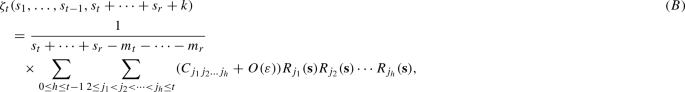
where the constants $C_{j_1j_2\ldots j_h}$ depend only on the main terms of (5.1) and do not depend on the last term of (5.1).

Proof of the Corollary

We use induction on t. We first prove the case $t=1$. $\square$

(Proof of ($A_1$).) Since $s_1+\cdots +s_r+k\lessapprox 0$ by type 1, we have $\zeta (s_1+\cdots +s_r+k)=\zeta (m_1+\cdots +m_r+k)+O(\varepsilon )=(C_{\phi }+O(\varepsilon ))R_{\phi }({\mathbf {s}})$ with $C_{\phi }= \zeta (m_1+\cdots +m_r+k)$. Hence ($A_1$) holds.

(Proof of ($B_1$).) When $s_1+\cdots +s_r+k\sim 1$, we have $k-1=-m_1-\cdots -m_r$, and so

$$\begin{aligned} \zeta (s_1+\cdots +s_r+k)&=\frac{1}{s_1+\cdots +s_r+k-1}+\gamma +O(\varepsilon )\\&=\frac{1+(\gamma +O(\varepsilon ))(\varepsilon _1+\cdots +\varepsilon _r)}{s_1+\cdots +s_r-m_1-\cdots -m_r}\\&=\frac{1}{s_1+\cdots +s_r-m_1-\cdots -m_r}(C_{\phi }+O(\varepsilon ))R_{\phi }({\mathbf {s}}) \end{aligned}$$

with $C_{\phi }=1$. When $s_1+\cdots +s_r+k > rapprox 2$, we have

$$\begin{aligned}&\zeta (s_1+\cdots +s_r+k)\\&\quad =\zeta (m_1+\cdots +m_r+k)+O(\varepsilon )\\&\quad =\frac{1}{s_1+\cdots +s_r-m_1-\cdots -m_r}(\varepsilon _1+\cdots +\varepsilon _r) (\zeta (m_1+\cdots +m_r+k)+O(\varepsilon ))\\&\quad =\frac{1}{s_1+\cdots +s_r-m_1-\cdots -m_r}(0+O(\varepsilon ))R_{\phi }({\mathbf {s}}). \end{aligned}$$

Hence $(B_1)$ holds.

Next, for $2\le t\le r$, we assume that ($A_{t-1}$) and ($B_{t-1}$) hold, and we prove ($A_t$) and ($B_t$).

For ${\mathbf {m}}\in ({\mathbb {Z}}_{\le 0})^r$ and $k\in {\mathbb {Z}}$, we take an integer M satisfying $k\le M-1$ and $M\ge M_r({\mathbf {m}})+1$. Then by (5.1), or rather (2.1), we have

$$\begin{aligned}&\zeta _t(s_1,\ldots ,s_{t-1},s_t+\cdots +s_r+k)\nonumber \\&\quad =\frac{1}{s_t+\cdots +s_r+k-1}\zeta _{t-1}(s_1,\ldots ,s_{t-2}, s_{t-1}+s_t+\cdots +s_r+k-1)\nonumber \\&\qquad +\sum _{k'=0}^{M-k-1}\left( {\begin{array}{c}-(s_t+\cdots +s_r+k)\\ k'\end{array}}\right) \zeta _{t-1}(s_1,\ldots ,s_{t-2},s_{t-1}+\cdots +s_r+k+k')\zeta (-k')\nonumber \\&\qquad +\frac{1}{\Gamma (s_t+\cdots +s_r+k)}I(s_1,\ldots ,s_{t-1}, s_t+\cdots +s_r+k;M-k-\eta )\nonumber \\&\quad =Z_1+Z_2+Z_3, \end{aligned}$$

(5.11)

say. Let us check that the integral included in $Z_3$ is convergent. It is enough to prove the inequality $M-k\ge M_t(m_1,\ldots ,m_{t-1},m_t+\cdots +m_r+k)+1$. In fact,

$$\begin{aligned}&M_t(m_1,\ldots ,m_{t-1},m_t+\cdots +m_r+k)+1\\&\quad =\max _{1\le j\le t}\{t-j-m_j-\cdots -m_{t-1}-(m_t+\cdots +m_r+k)\}+1\\&\quad =\max _{1\le j\le t}\{r-j-m_j-\cdots -m_r\}+t-r-k+1\\&\quad =\max _{1\le j\le r}\{r-j-m_j-\cdots -m_r\}+t-r-k+1 \end{aligned}$$

(where the last equality is because the quantity in the curly parentheses is monotonically decreasing with respect to j), and hence the right-hand side is

$$\begin{aligned} =M_r({\mathbf {m}})+t-r-k+1\le M-k. \end{aligned}$$

We further divide $Z_2$ into two parts as

$$\begin{aligned} Z_2&=\sum _{\begin{array}{c} 0\le k'\le M-k-1 \\ s_{t-1}+\cdots +s_r+k+k'\lessapprox 0 \end{array}} \left( {\begin{array}{c}-(s_t+\cdots +s_r+k)\\ k'\end{array}}\right) \nonumber \\&\quad \times \zeta _{t-1}(s_1,\ldots ,s_{t-2},s_{t-1} +\cdots +s_r+k+k')\zeta (-k')\nonumber \\&\quad +\sum _{\begin{array}{c} 0\le k'\le M-k-1 \\ s_{t-1}+\cdots +s_r+k+k' > rapprox 1 \end{array}} \left( {\begin{array}{c}-(s_t+\cdots +s_r+k)\\ k'\end{array}}\right) \nonumber \\&\quad \times \zeta _{t-1}(s_1,\ldots ,s_{t-2},s_{t-1}+\cdots +s_r+k+k') \zeta (-k')\nonumber \\&=Z_{21}+Z_{22}, \end{aligned}$$

(5.12)

say. The first part $Z_{21}$ corresponds to type 1 and the second part $Z_{22}$ corresponds to type 2.

(Proof of ($A_t$).) We prove that $Z_1,Z_{21},Z_{22}$, and $Z_3$ have the expression of the right-hand side of (A). Since we consider the case of type 1, $s_t+\cdots +s_r+k-1\lessapprox -1$ holds, so $Z_1$ has the expression of (A) by the induction hypothesis. The term $Z_{21}$ also has the expression of (A) since variables of all $\zeta _{t-1}$ are of type 1. The variables in $Z_{22}$ are of type 2. Hence $\zeta _{t-1}$ has the factor $(s_{t-1}+\cdots +s_r-m_{t-1}-\cdots -m_r)^{-1}$ by the assumption. On the other hand, the binomial coefficient

$$\begin{aligned}&\displaystyle \left( {\begin{array}{c}-(s_t+\cdots +s_r+k)\\ k'\end{array}}\right) \\&\quad \displaystyle =\frac{(-(s_t+\cdots +s_r+k)) \cdots (-(s_t+\cdots +s_r+k)-k'+1)}{k'!} \end{aligned}$$

has the factor $(s_{t}+\cdots +s_r-m_{t}-\cdots -m_r)\sim 0$ since the numerator is the product of factors from $-(s_t+\cdots +s_r+k) > rapprox 0$ to

$$\begin{aligned} -(s_t+\cdots +s_r+k)-k'+1=s_{t-1}-(s_{t-1}+s_t +\cdots +s_r+k+k'-1)\lessapprox 0. \end{aligned}$$

Therefore $Z_{22}$ has a factor

$$\begin{aligned} \frac{s_t+\cdots +s_r-m_t-\cdots -m_r}{s_{t-1}+\cdots +s_r-m_{t-1} -\cdots -m_r}=R_t({\mathbf {s}}), \end{aligned}$$

and so $Z_{22}$ has the expression of (A) by the assumption. The term $Z_3$ can be written as $(0+O(\varepsilon ))R_{\phi }({\mathbf {s}})$ since the gamma function has a pole at $m_t+\cdots +m_r+k$.

(Proof of ($B_t$).) Under the condition $m_t+\cdots +m_r+k\ge 1$, we prove that $Z_1$, $Z_{21}$, $Z_{22}$, and $Z_3$ has the expression of the right-hand side of (B). When $m_t+\cdots +m_r+k=1$, $Z_1$ is

$$\begin{aligned} \frac{1}{s_t+\cdots +s_r-m_t-\cdots -m_r}\zeta _{t-1}(s_1, \ldots ,s_{t-2},s_{t-1}+s_t+\cdots +s_r+k-1). \end{aligned}$$

Since $s_{t-1}+s_t+\cdots +s_r+k-1\lessapprox 0$, $\zeta _{t-1}$ has the expression of (A), so $Z_1$ can be written in the form (B) in this case. When $m_t+\cdots +m_r+k\ge 2$ and $s_{t-1}+s_t+\cdots +s_r+k-1\lessapprox 0$, $\zeta _{t-1}$ has the expression (A) by ($A_{t-1}$) and $Z_1$ is represented as

$$\begin{aligned}&\frac{1}{s_t+\cdots +s_r-m_t-\cdots -m_r} \frac{s_t+\cdots +s_r-m_t-\cdots -m_r}{s_t+\cdots +s_r+k-1}\\&\quad \times \zeta _{t-1}(s_1,\ldots ,s_{t-2},s_{t-1}+s_t+\cdots +s_r+k-1). \end{aligned}$$

Hence in this case, $Z_1$ can be written in the form (B). When $m_t+\cdots +m_r+k\ge 2$ and $s_{t-1}+s_t+\cdots +s_r+k-1 > rapprox 1$, $Z_1$ is represented as

$$\begin{aligned}&\frac{1}{s_t+\cdots +s_r-m_t-\cdots -m_r}\frac{1}{s_t+\cdots +s_r+k-1}\\&\quad \times \frac{s_t+\cdots +s_r-m_t-\cdots -m_r}{s_{t-1} +\cdots +s_r-m_{t-1}-\cdots -m_r} (s_{t-1}+\cdots +s_r-m_{t-1}-\cdots -m_r)\\&\quad \times \zeta _{t-1}(s_1,\ldots ,s_{t-2},s_{t-1}+s_t+\cdots +s_r+k-1). \end{aligned}$$

The denominator $s_t+\cdots +s_r+k-1$ is $\not \sim 0$ and the factor

$$\begin{aligned} (s_t+\cdots +s_r-m_t-\cdots -m_r)/(s_{t-1}+\cdots +s_r-m_{t-1}-\cdots -m_r) \end{aligned}$$

is $R_t({\mathbf {s}})$. Moreover

$$\begin{aligned} (s_{t-1}+\cdots +s_r-m_{t-1}-\cdots -m_r)\zeta _{t-1}(s_1,\ldots ,s_{t-2}, s_{t-1}+s_t+\cdots +s_r+k-1) \end{aligned}$$

can be written in the form (A) even though $\zeta _{t-1}$ has the expression (B) by ($B_{t-1}$). Therefore also in this case, $Z_1$ can be written in the form (B).

Since $Z_{21}$ has the expression of (A), multiplying by the factors

$$\begin{aligned} \frac{1}{s_t+\cdots +s_r-m_t-\cdots -m_r}\cdot (s_t+\cdots +s_r-m_t-\cdots -m_r), \end{aligned}$$

(5.13)

we see that $Z_{21}$ can be represented by the form (B). The term $Z_{22}$ has the factor $1/(s_{t-1}+\cdots +s_r-m_{t-1}-\cdots -m_r)$ since $\zeta _{t-1}$ satisfies ($B_{t-1}$). Multiplying by (5.13), we obtain the factor $1/(s_t+\cdots +s_r-m_t-\cdots -m_r)R_t({\mathbf {s}})$, so $Z_{22}$ can also be represented by the form (B).

Finally we estimate $Z_3$. By multiplying it by (5.13), we have

$$\begin{aligned} Z_3=\frac{1}{s_t+\cdots +s_r-m_t-\cdots -m_r}(0+O(\varepsilon )) R_{\phi }({\mathbf {s}}), \end{aligned}$$

hence this term has the expression (B). $\square$

References

Akiyama, S., Egami, S., Tanigawa, Y.: Analytic continuation of multiple zeta-functions and their values at non-positive integers. Acta Arith. 98, 107–116 (2001)
Akiyama, S., Tanigawa, Y.: Multiple zeta values at non-positive integers. Ramanujan J. 5, 327–351 (2001)
Berndt, B.C.: Ramanujan’s Notebooks, Part I. Springer, New York (1985)
Fuks, B.A.: Theory of Analytic Functions of Several Complex Variables, Transl. Math. Monographs, vol. 8. Amer. Math. Soc., Providence (originally written in Russian, Moscow) (1963)
Hoffman, M.E.: Multiple harmonic series. Pac. J. Math. 152, 275–290 (1992)
Komori, Y.: An integral representation of multiple Hurwitz-Lerch zeta functions and generalized multiple Bernoulli numbers. Q. J. Math. (Oxf.) 61, 437–496 (2010)
Matsumoto, K.: On the analytic continuation of various multiple zeta-functions. In: Bennett, M.A., Peters, A.K., Natick et al. (eds.) Number Theory for the Millennium II, Proc. Millennial Conf. on Number Theory, pp. 417–440. A K Peters, (2002)
Matsumoto, K.: Asymptotic expansions of double zeta-functions of Barnes, of Shintani, and Eisenstein series. Nagoya Math. J. 172, 59–102 (2003)
Matsumoto, K.: The analytic continuation and the asymptotic behaviour of certain multiple zeta-functions I. J. Number Theory 101, 223–243 (2003)
Matsumoto, K., Tsumura, H.: Mean value theorems for the double zeta-function. J. Math. Soc. Jpn. 67, 383–406 (2015)
Onozuka, T.: Analytic continuation of multiple zeta-functions and the asymptotic behavior at non-positive integers. Funct. Approx. Comment. Math. 49, 331–348 (2013)
Osgood, W.F.: Lehrbuch der Funktionentheorie, Zweiter Band, Erste Lieferung. Teubner, Leibzig, 1929, Reprint: Chelsea (1965)
Sasaki, Y.: Multiple zeta values for coordinatewise limits at non-positive integers. Acta Arith. 136, 299–317 (2009)
Sasaki, Y.: Some formulas of multiple zeta values for coordinate-wise limits at non-positive integers. In: R. Steuding and J. Steuding (eds.) New Directions in Value-Distribution Theory of Zeta and \(L\)-Functions, Proc. Würzburg Conf., Shaker, Aachen, pp. 317–325 (2009)
Zagier, D.: Values of zeta functions and their applications. In: Joseph, A. et al. (eds.) First European Congress of Mathematics, vol. II, Progr. Math., vol. 120, Birkhäuser, Basel, pp. 497–512 (1994)
Zhao, J.: Analytic continuation of multiple zeta functions. Proc. Am. Math. Soc. 128, 1275–1283 (2000)
Author information
Authors and Affiliations
Corresponding author
Additional information
Publisher's Note
Springer Nature remains neutral with regard to jurisdictional claims in published maps and institutional affiliations.
This research was partially supported by Grants-in-Aid for Scientific Research, Grant numbers 25287002 (for the first-named author) and 13J00312 (for the second-named author), JSPS.