1. Introduction
Developing efficient, cost competitive and survivable wave energy converters (WECs), has proven, in the last years, to be a challenging task [
1,
2,
3]. Fluid dynamic analyses are fundamental at every design stage to evaluate the behaviour of the WEC [
4], so different methods for simulating the fluid forces and the interaction between waves and semi-submerged bodies have been developed, with increasing levels of fidelity and associated computational cost. Solving the complete set of Navier–Stokes Equations (NSE) for offshore engineering applications is expensive and not advised because the computational cost is too high compared to the accuracy desired [
5]. Therefore, the NSE are simplified to obtain a linear equivalent potential flow theory (PF), where the solution is obtained through linearization, thanks to assumptions of inviscid fluid and irrotational, incompressible flow. In this way, one of the most complex set of equations is transformed into a Laplace problem. Under such hypotheses, the Boundary Element Method (BEM) can be implemented, which is a numerical approach for the solution of linear partial differential equations, expressed as integral equations. BEM represents a valid alternative to Reynolds Average Navier–Stokes (RANS) simulation: Being three (or more) orders of magnitude faster [
6], BEM is used in many industrial and research applications, especially when computational resources are limited and accuracy is not of primary importance. Linear approaches produce satisfactory results when modelling linear waves and the WEC is moving around the operative point. In fact, non linearities of fluid forces are less important when oscillations are small and smooth. The success of linear models is justified by their many perks, which include, but not limited to, extreme simplicity, compliance with the superposition principle and great flexibility that makes them compatible with a vast array of mathematical tools. The linearization is always referred to the operating point. In many applications this is a reasonable assumption, since the working condition is not far respect a specific setpoint; in contrast, in the case of wave energy conversion, the objective is to drive the system as far away from equilibrium as possible, in order to maximize the produced energy. This is likely to excite nonlinear dynamics, resulting in non-representative linear models, which usually underestimate energy losses and overestimate the productivity of the WEC [
7].
Two main assumptions must be satisfied when using BEMs:
The better these hypotheses are met, the higher the accuracy of the results obtained with the linear model [
8]. Although linear PF methods have been used successfully in many offshore engineering applications, the linearizing assumptions are often challenged by realistic WEC behaviour, where large amplitude motions result in viscous drag, flow separation, vortex shedding and other nonlinear hydrodynamic effects [
5]. In order to improve the linear time domain model of a WEC, described by the Cummins’ equation [
9], it is possible to include a viscous damping term as an external force, without significantly increment the computational time required to run the model. In this paper, a notional un-coupled linear and quadratic dependence of the viscous force on the velocity is assumed, hence considering two additive terms. It follows that two viscous drag coefficients should be identified, one for the linear contribution and one for the quadratic contribution. The addition of such non-linear damping force is necessary to avoid divergence in simulations under certain conditions: for example, the model of a forced, undamped system, is likely to explode into very large, non-realistic motion close to resonance conditions. Diverging behaviour can happen without a proper extinction coefficient and is not possible to model some of the conditions the WEC will face at sea [
10].
A way to determine damping coefficients is to conduct an experimental campaign, analysing the free decay motion of the WEC [
11,
12]. For each degree of freedom (DOF), the WEC is released from a set of initial conditions in order to highlight when non-linearities become important; this test is usually performed to identify the roll damping for ships [
13]. In order to consider only the significant kinematics of the free decay, the analysed time trace usually covers a few oscillations before the transient elapses; for different starting conditions, the resulting angular acceleration, velocity and rotation angle are post-processed to estimate damping parameters. However, experimental campaigns [
14] are expensive and usually not affordable in the early design stage of a WEC. Such a critical obstacle can be overcome by using the use of a CFD Numerical Wave Tank (CNWT). CFD is a Hi-Fi approach to the problem that makes the inclusion of all non-linearities possible. However, CFD is so computationally expensive that it cannot be used for extensive analysis or study of operative conditions: Its most common use is when large non-linearities are expected (survivability, large motion) or for tuning and validating lower-fidelity models, or investigating behaviour of related devices such as tuning tanks [
15]. Furthermore, turbulence is a critical feature to handle. There are mainly three techniques to deal with it: Direct Numerical Simulations (DNS), in such simulations, all of the motions contained in the flow are resolved, Large Eddy Simulations (LES) in which NSEs are filtered over the space, finally RANS in which flow quantities are split into the mean value and the perturbation. The resulting equations of LES and RANS are essentially identical, the difference is that in LES most of the turbulence energy is resolved [
16]. The URANS approach is chosen because it is the best cost-efficient method considering accuracy and solver time (which could increase easily by several orders of magnitude from RANS to LES and DNS).
The aim of this paper is to define a CFD setup able to emulate a real tank experiment and to describe a methodology to identify the viscous damping coefficients along the two rotational DOFs of a WEC, namely pitch and roll. In particular, the WEC is a prismatic pitching platform that extracts energy from the pitching motion. On the one hand, viscous losses in pitch are detrimental for power extraction, since they increase the dissipation in the DOF exploited to harvest energy; on the other hand, roll response to oblique or short-crested waves is also detrimental, since it absorbs part of the incoming energy, hence decreasing the energy available to the pitch DOF. Therefore, it is important to obtain a reliable prediction of both pitch and roll responses. The goal of this paper is to increase the fidelity of models based on the potential flow theory by adding the effect of viscous non-linearities. It is worthwhile to remark that most of the literature in the wave energy field is concerned with the identification of viscous losses in the DOF used for energy extraction only (usually a smooth surfaces), while ancillary DOFs are often neglected (with sharp edges in the case study herein considered). Hence, this paper also purports to discuss specific challenges and intrinsic differences between different DOFs, despite using the same test-case and identification technique. Results carried out from simulations are consistent with expectations based on the shape of the hull: the linear term of the damping force prevails in the pitch free decay analysis while the quadratic term, that models the viscous non-linearities, is predominant in the roll DOF.
This paper is organized as follows. After a brief presentation of the device considered in
Section 2, the mathematical model of the methodology presented in this paper is discussed in
Section 3. The CFD simulation and its setup is explained in
Section 4 with emphasis on damping techniques to avoid wave reflections and overset mesh. In the final part of CFD section the mesh convergence study is presented and discussed. Results of simulations are shown in
Section 5, firstly as regards CFD scenes, then kinematics and finally the application of methodology discussed in the mathematical section. Ultimately the conclusions of
Section 6 involve the analysis of the previously shown outcomes and a last post-processing phase by solving the equation of motion in the time domain, including the non-linear damping effect and the optimization of coefficient identification through the goodness of fit.
3. Mathematical Model and Identification Method
The time domain linear model of a floating WEC is based on the Cummins’ equation [
9].
where the terms of Equation (
1) are:
is the matrix of added mass at infinite frequency
M is the mass matrix
is the external force
K is the stiffness matrix
is the radiation impulse response function
The convolution term represents, along with , the effect of wave radiation in an ideal fluid and it is often referred to as fluid memory effect, because it considers the energy of the radiated waves due to the past motion of the body.
The hydrodynamic parameters in Equation (
1) are computed via BEM-based software (e.g., NEMOH [
17] and ANSYS Aqwa [
18]). It is worth noting that in Equation (
1) there are no linearity limitations on the external forces, hence the model is potentially capable to deal with non-linear contributions. Viscous effects are modelled via the addition of a nonlinear term to the right-hand side of Equation (
1), divided into linear and quadratic dependence on the pitching velocity
.
The identification of such damping parameter is conducted using the logarithmic-decrement decay method [
11,
12,
19], which considers the rate of decay of oscillation starting from a non-equilibrium position. During a free decay test, the system oscillates, for each DOF, at its single natural frequency, thus it is possible to determine both the natural period and the hydrodynamic damping. The non-linear equation for free decay pitch motion is:
where the subscript 55 refers to the pitching DOF,
is the pitch angle and the frequency-dependent added mass
A is calculated at the natural frequency of the system (
).
is the nonlinear viscous force, defined as
where
is the coefficient for linear dissipation, and
is the coefficient for quadratic dissipation. Note that
accounts for both linear viscous damping and radiation damping. Equation (
3) can be directly included in a non-linear time domain model, with the coefficients
and
identified as the ones that minimize the error between a fidelity-benchmark (CFD, for instance) and the time-domain model. However, it is often crucial to preserve the linear structure of the lower-fidelity model, for example to retain the ability to simulate the model in the frequency domain. Therefore, it is useful to linearize Equation (
3), while preserving the ability to discriminate between linear and quadratic contributions. According to [
20], it is possible to assume that for each half-cycle, the oscillation is reasonably sinusoidal. Under such an assumption, the non-linear (quadratic) term of Equation (
3) can be linearized using the Fourier series expansion:
where
and
are the amplitude and the frequency of oscillation of the
i-th oscillation cycle, respectively. Consequently, the linearized damping force can be defined as:
With the inclusion of
and dividing Equation (
2) by the equivalent inertia
, it is possible to obtain the non-dimensional linear equation of motion in the canonical form:
where
with
and
. Equation (
6) describes a linear underdamped system, for which the envelope curve of a decay starting from
is defined as:
Applying Equation (
8) for two consecutive peaks
i and
of the decay curve, it is possible to calculate the logarithmic decay:
Thus, identifying the equivalent linear extinction coefficient:
where
and the damped natural pitch frequency can be calculated as:
This method allows to calculate the extinction curve of the
as a function of the mean amplitude
for each cycle. To exploit all the available experimental data and obtain a more accurate estimation, it is possible to calculate
and
for each oscillation cycle, considering both maxima and minima peaks and grouping the informations of all the decay tests for the specific DOF. The linear regression fit is then performed on the calculated points, with respect to the curve expression:
which allows to identify the linear and quadratic extinction coefficients:
4. CFD Model
The analysis has been carried out on the commercial software Star-CCM+ from Siemens [
21] and a Unsteady Reynold Average Navier–Stokes (URANS) approach has been used. Particular attention should be paid to the setup of the CFD simulation environment, since different fluid interfaces, fluid-structure interaction and large solid body motion present numerical problems of challenging resolution. Under such conditions, reliable results can only be achieved by an appropriate and comprehensive model definition. The following subsections detail the most relevant aspects to take under consideration when performing pitch and roll free decay tests of a floating pitching platform as the one considered in this paper.
4.1. Domain, Boundary Conditions and Damping Length
Due to its oscillation, the floater generates radiated waves that propagate towards the boundaries of the domain, effectively dissipating energy. In order to correctly represent the amount of energy that is subtracted from the floater due to wave generation, it is crucial to capture the wave pattern generated by the hull during the oscillations. In this regard, the domain needs to be large enough to contain the most energetic part of the wave pattern, freely propagating in each direction. Considering and , respectively length and width of the hull, domain overall length is and its width . Since the wave are generated by the hull of length , depth of domain is set to in order to respect the deep water approximation .
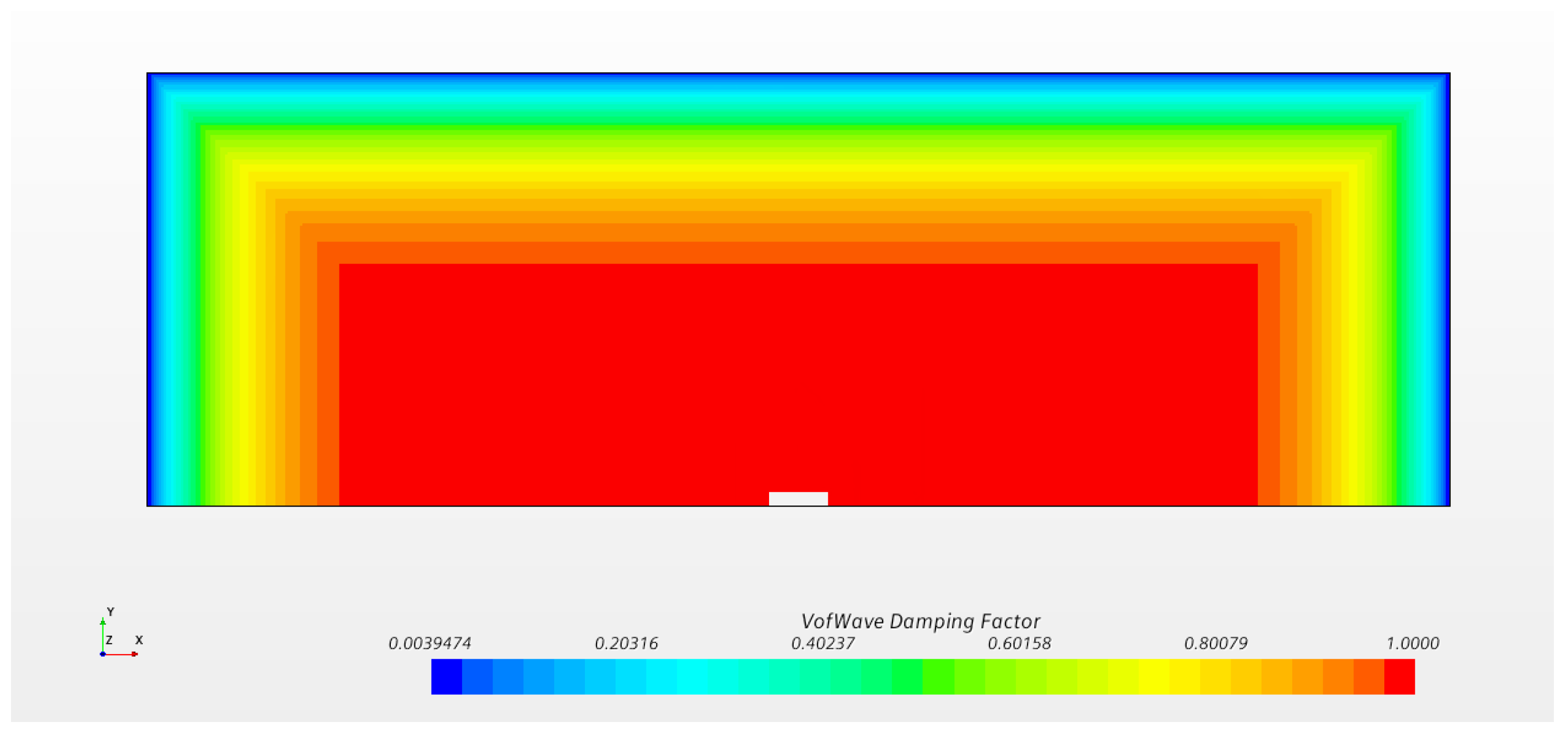
The choice of the dimensions of the domain also depends on wave reflection phenomena, which are a critical problem in both real and numerical tanks. In fact, reflected waves modify the wave field and ultimately affect the dynamics of the floater; Furthermore, it is difficult, if not impossible, to accurately separate the contribution of radiated and reflected waves, leading to improper measures, in case of real experiments, and to numerical noise and simulation crash, in case of numerical tanks. A possible solution consists in adding a damping zone at the boundaries of the domain in order to decrement the energy and the height of waves before they reach the frontier of the domain. Therefore, damping zones hinder the generation of reflected waves, leaving fluid domain perturbed mainly by the radiated waves for the whole duration of the significant decay.
The damping zone should have an appropriate length (at least twice the wavelength [
21]) and intensity of the damping [
22]. Damping waves is possible by introducing an additional resistance term
as a source into the momentum equation relative to the vertical motion
w, according to [
22]:
where:
is the starting point for wave damping (along x-axis direction)
is the end point (i.e., the boundary)
is the water density
w is the vertical velocity component
,
and
n are parameters of the damping model of Choi et al. [
22].
In this particular case, considering a wavelength (
) comparable to the hull’s length, considering the results of Peric et al. [
23] and after a trial-and-error evaluation stage, based on estimation of the simulation’s residuals, the following values have been imposed:
Bearing this in mind, the waves reflection phenomenon has been addressed imposing a damping factor
k in Equation (
17) within a distance of 20 m from the boundaries as shown in
Figure 2, that represents a top-view of the sea surface of the simulation.
The boundaries conditions are shown in
Figure 3. With respect to the boundaries named
top and
bottom, they are set as
velocity inlet, because a unique phase, air and water, respectively, with zero-velocity is imposed. At
side,
right and
left, the boundary conditions are set as
pressure outlet, and the pressure is forced to be the atmospheric one for the air section and the hydrostatic one for the water part.
Being the domain a function of wavelength, a parametric approach has been used: For the different free decay tests and different initial conditions the wave produced are quite various and so the domain and mesh refinements, to maximize efficiency of the simulation.
4.2. Mesh Generation
In CFD there are two ways to deal with moving bodies: Mesh morphing/remeshing techniques are best when the movement of the body is very small, while they are too computationally expensive and potentially unstable with large displacements of the floater, since the mesh morphing task becomes a significant portion of the overall computational burden. Alternatively, when large motions are expected, overset methods should be preferred [
24,
25]. Thus the overset approach has been chosen for this study and the domain is split in two different overlapped parts: background and overset. The overset is the one moving with the body, while the background is fixed. With the overset approach, no remesh operation is needed because the mesh never deforms nor its quality decreases, since it moves with the body and remains unaltered. The overset and background separate regions exchange information due to an overlapping area consisting of some cells, called donor and acceptor, where the solution is interpolated trough Chimera Interpolation techniques according to [
26,
27]. Equations are solved separately in these different areas and bound together only at the interface between the two zones.
While the dimensions of the background are function of the wavelength, the dimensions of the overset region are constant for all the tests because they are referred to the hull and not to the wave pattern. Another important volumetric refinement is the one around the overset which ensures that, in the zone where information are exchanged, cells belonging to overset and background have the same volume, in order to reduce discretization and interpolation errors. When dealing with trimmed block mesh, it is is important to bear in mind that cells can increase their size only by double.
4.2.1. Tank
A trimmed mesh has been chosen due to the possibility to create anisotropic cells which provide a predominantly hexahedral mesh with minimal cell skewness, it results as the best discretization at the interface between the two fluids. It is worthwhile to remark that wave reflection can occur also when the mesh size suddenly changes. To avoid this problem, usually three different volumetric sea surface refinements are used in order to gradually coarsen the mesh, as shown from a prospective-side view in
Figure 4 and side-view in
Figure 5.
The wave damping should start before the coarsest grid level is reached since such a change in cell size is a potential source of reflection that should be included in the damping zone [
28].
4.2.2. Overset Region
Two main factors influence the overset’s dimensions:
Overset does not have to be too large, otherwise the extremities will move too much when it rotates, generating interpolation errors and requiring a lower time step
Neither too small, because cells need space to grow from the wall to the interfaces; Moreover this guarantees that the strongest gradients are solved within the overset and not in the zone where information is exchanged.
For the overset sea refinement, we used the shape displayed in
Figure 6 and isotropic cells because, otherwise, when the region rotates, the anisotropic sea refinement at the water line will rotate along with the hull.
4.3. Volume of Fluid
The Volume of Fluid (VOF) Multiphase model is an Eulerian numerical model suited to simulate flows of several immiscible fluids on numerical grids, capable of resolving the interface between the different phases [
29]. The spatial distribution of each phase at a given time is defined in terms of a variable that is called the volume fraction. A method of calculating such distributions is to solve a transport equation for the phase volume fraction. The method uses the STAR-CCM+ Segregated Flow model which solves each of the momentum equations in turn. The VOF Multiphase model is the standard model to deal with marine environment and wave generation in a RANS simulation [
21].
4.4. Turbulence, Wall Treatment, Y+
K-Epsilon is a two-equations model that solves transport equations for the turbulent kinetic energy and the turbulent dissipation rate in order to determine the turbulent eddy viscosity. Such model provides a good compromise between robustness, computational cost and accuracy and are well suited for external flows and when gradients at wall are not too strong [
30,
31]. In our case a Realizable Two layer K-Epsilon Model is used [
32]. This model contains a new transport equation for the turbulent dissipation rate with respect to standard K-Epsilon. In addition, the turbulent viscosity is expressed as a function of mean flow and turbulence properties, rather than assumed to be constant as in the standard model. A two-layer wall treatment is adopted: this method solves for but prescribes and turbulent viscosity algebraically with distance from the wall in the viscosity-dominated near-wall flow regions. In this approach, the boundary layer is divided into two layers. The values specified in the near-wall layer are blended smoothly with the values computed from solving the transport equation far from the wall. The equation for the turbulent kinetic energy is solved across the entire flow domain. The two-layer approach, which resolves correctly for both low and high
, using respectively standard wall function and blended wall function according to Reichardt’s law [
33], fits perfectly with the free decay problem: after few oscillations the velocities are smaller and
value decreases during the numerical experiment. Based on such considerations, a target value of
has been chosen, since the aim of this work is to define damping coefficient accounting for non-linear effects, thus it is important to describe properly the boundary layer zone where viscous stress, separation or vortex shedding that occur. The value of
is obtained considering the flat-plate boundary layer theory [
34], obtaining a first cell height of
, considering a reasonable total thickness of
and using a number of 10 layers, which guarantee a smooth grow rate of the cells.
4.5. Time Step
In Star-CCM+ the multiphase VOF model requires the use of an implicit unsteady approach. A second order time-marching discretization has been chosen since the first order is numerically dissipative and the property of the wave may not be transported correctly. First order time discretization is the only model unconditionally stable, but it has a drawback: the leading term of the truncation error of convective flux resembles a diffusive flux. This numerical, or artificial, diffusion that is introduced in the solution is magnified in multidimensional problems if the flow is oblique to the grid. A very fine grid would be necessary to obtain accurate solutions. On the other hand, since a second order approach does not require such a refined mesh-discretization, it is faster and more accurate than a first-order time-discretization. Time step is limited by two different conditions:
The courant number at the interface between the two fluids has to be at least less than 1 (required by the VOF model), although it is suggested to keep it less than 0.5 in order to have a clean separation of the two fluids.
The movement of the overset cells at the interface between the two regions must be less than half the minimum cell size, when using a second order temporal scheme, in order to prevent overset mesh problems due to the exchange of information.
The more severe limitation on the time step comes from the latter condition; therefore, it is convenient to change the time step according to the different initial conditions: since the oscillation period is always the same, the further away from equilibrium is the initial displacement, the smaller the time step needs to be in order to maintain the same courant number.
4.6. Mesh Convergence Study
In order to support the goodness of the numerical scheme created, a grid independence analysis has been carried out. This process proves the stability of the numerical method and ensures that solution does not change when refining the mesh. This convergence study is based on the number of cells used to discretize the wave height that is generated by the oscillations of the hull. In the wave pattern there is the energy lost by the device during the free decay and it is fundamental to capture it accurately. Moreover, prism layer properties are base size independent and computed as absolute values, thus base size has little influence in the overall mesh. The number of layers that are necessary to discretize the wave is very dependent on wave steepness; according to [
5], at least 10 layers are suggested and even more for a sharp interface between fluids. Not using enough cells some information may be lost and wave transport and generation may be inaccurate, resulting in overly-damped or magnified waves. Cells count is very dependent on the number of layers of sea refinement because most of the cells come from this mesh control and from the overset zone, as confirmed by results presented in
Figure 7.
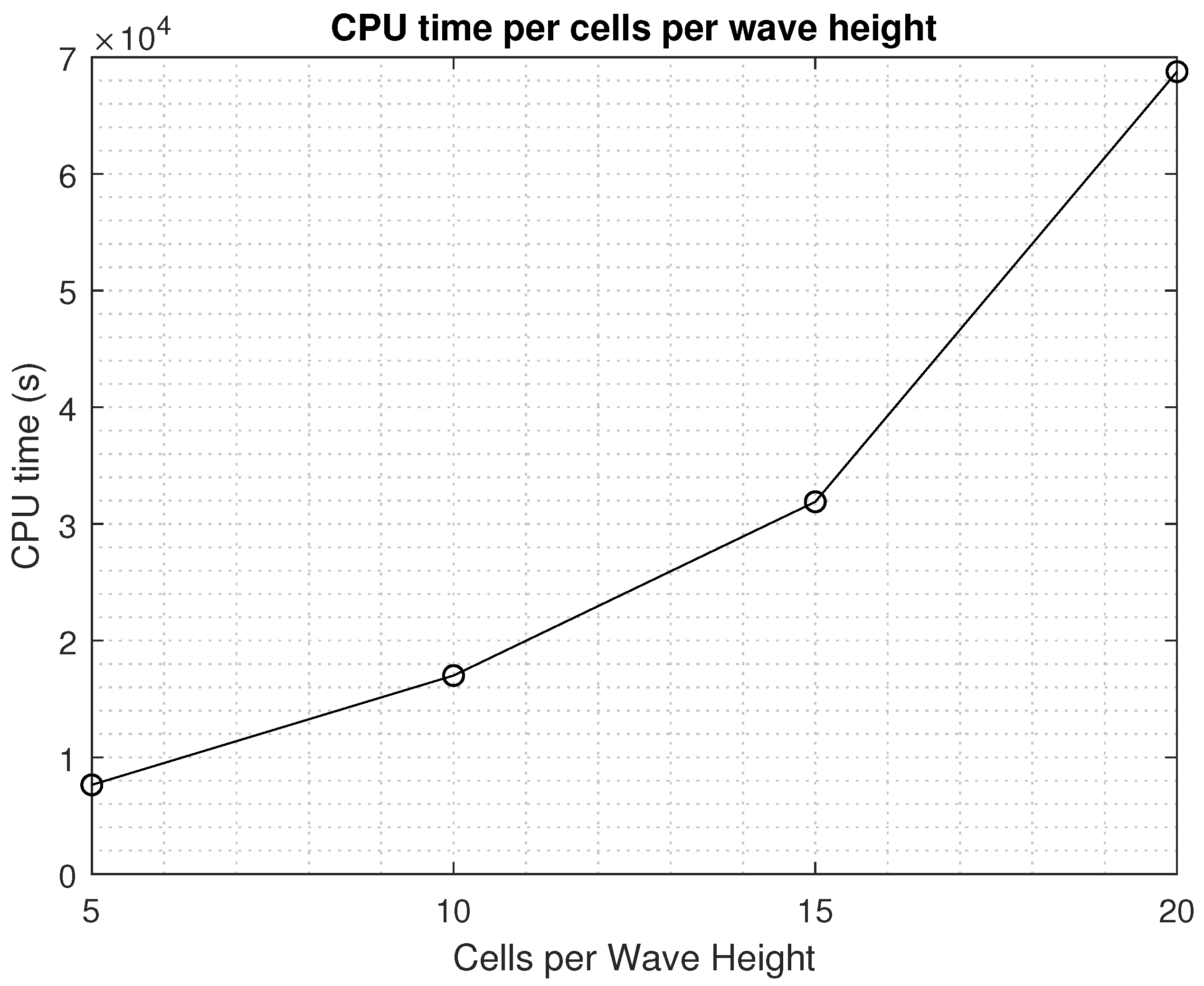
In order to choose the appropriate mesh sizes CPU time is considered, as shown in
Figure 8: passing from 15 cells to 20 means an increase of about 115%. So the configuration of 20 cells per wave height has been excluded because of the prohibitive computational time.
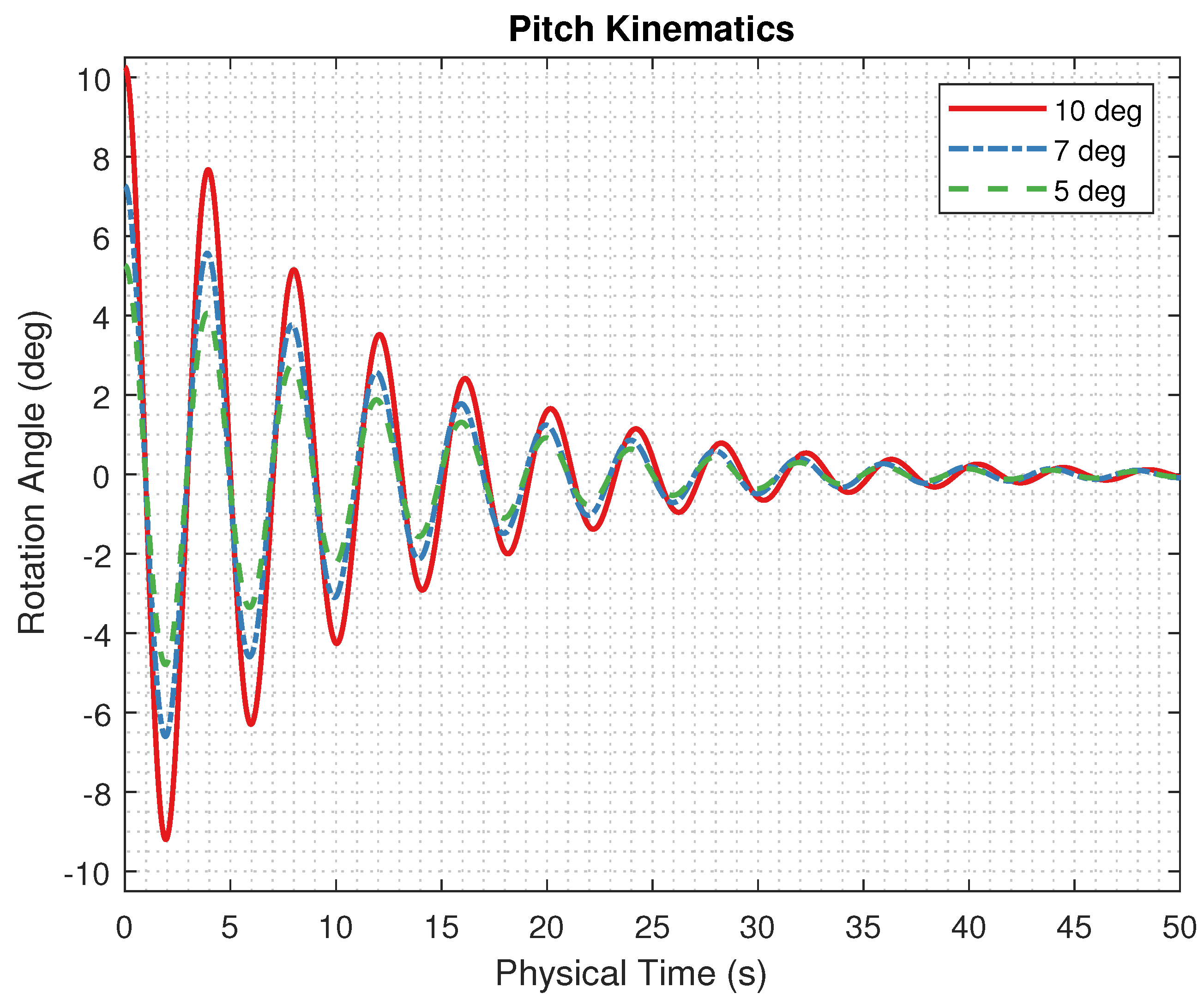
The cells count of the overset is related with the size of the sea refinement, because cells at the interface between background and overset must have same volume, especially at sea surface. Convergence study is done on the kinematics of the free decay with respect to
Figure 9, which is also the data used for the post-processing and evaluation of damping coefficients.
The wave height with several probes has also been monitored in order to understand the impact of mesh resolution in areas far from the floater.
The coarsest mesh setups have been compared to the finest ones corresponding to 20 cells in terms of relative errors and the associated root-mean-square as shown in
Figure 10 and
Figure 11.
Finally, 15 cells per wave height have been chosen, in order to ensure a good compromise between wave capturing and computational cost specially considering the trend of errors in
Figure 10, the low related rms (
Figure 11) and its computational cost in terms of time (
Figure 8).

 ,
, 


