On the edge of the stable range

Abstract

We prove a general homological stability theorem for certain families of groups equipped with product maps, followed by two theorems of a new kind that give information about the last two homology groups outside the stable range. (These last two unstable groups are the ‘edge’ in our title.) Applying our results to automorphism groups of free groups yields a new proof of homological stability with an improved stable range, a description of the last unstable group up to a single ambiguity, and a lower bound on the rank of the penultimate unstable group. We give similar applications to the general linear groups of the integers and of the field of order 2, this time recovering the known stability range. The results can also be applied to general linear groups of arbitrary principal ideal domains, symmetric groups, and braid groups. Our methods require us to use field coefficients throughout.

1 Introduction

A sequence of groups and inclusions $G_1\hookrightarrow G_1\hookrightarrow G_3\hookrightarrow \cdots$ is said to satisfy homological stability if in each degree d there is an integer $n_d$ such that the induced map $H_d(G_{n-1})\rightarrow H_d(G_n)$ is an isomorphism for $n> n_d$. Homological stability is known to hold for many families of groups, including symmetric groups [21], general linear groups [4, 22, 29], mapping class groups of surfaces and 3-manifolds [14, 18, 25, 30], diffeomorphism groups of highly connected manifolds [12], and automorphism groups of free groups [16, 17]. Homological stability statements often also specify that the last map outside the range $n> n_d$ is a surjection, so that the situation can be pictured as follows.

$$\begin{aligned} \cdots \rightarrow H_d(G_{n_d-3}) \rightarrow \underbrace{ H_d(G_{n_d-2}) \rightarrow H_d(G_{n_d-1}) }_{\text {edge of the stable range}} \twoheadrightarrow \underbrace{ {H_d(G_{n_d})} \xrightarrow {\cong } {H_d(G_{n_d+1})} \xrightarrow {\cong } \cdots }_{\text {stable range}} \end{aligned}$$

The groups $H_d(G_{n_d}), H_d(G_{n_d+1}),\ldots$, which are all isomorphic, are said to form the stable range. This paper studies what happens at the edge of the stable range, by which we mean the last two unstable groups $H_d(G_{n_d-2})$ and $H_d(G_{n_d-1})$. We prove a new and rather general homological stability result that gives exactly the picture above with $n_d=2d+1$. Then we prove two theorems of an entirely new kind. The first describes the kernel of the surjection $H_d(G_{n_d-1})\twoheadrightarrow H_d(G_{n_d})$, and the second explains how to make the map $H_d(G_{n_d-2})\rightarrow H_d(G_{n_d-1})$ into a surjection by adding a new summand to its domain. These general results hold for homology with coefficients in an arbitrary field.

We apply our general results to general linear groups of principal ideal domains (PIDs) and automorphism groups of free groups. In both cases we obtain new proofs of homological stability, recovering the known stable range for the general linear groups, and improving upon the known stable range for $\mathrm {Aut}(F_n)$. We also obtain new information on the last two unstable homology groups for $\mathrm {Aut}(F_n)$, $GL _n(\mathbb {Z})$ and $GL _n(\mathbb {F}_2)$, in each case identifying the last unstable group up to a single ambiguity.

Our proofs follow an overall pattern that is familiar in homological stability. We define a sequence of complexes acted on by the groups in our family, and we assume that they satisfy a connectivity condition. Then we use an algebraic argument, based on spectral sequences obtained from the actions on the complexes, to deduce the result. The connectivity condition has to be verified separately for each example, but it turns out that in our examples the proof is already in the literature, or can be deduced from it. The real novelty in our paper is the algebraic argument. To the best of our knowledge it has not been used before, either in the present generality or in any specific instances. Even in the case of general linear groups of PIDs, where our complexes are exactly the ones used by Charney in the original proof of homological stability [4] for Dedekind domains, we are able to improve the stable range obtained, matching the best known.

1.1 General results

Let us state our main results, after first establishing some necessary terminology. From this point onwards homology is to be taken with coefficients in an arbitrary field $\mathbb {F}$, unless stated otherwise.

A family of groups with multiplication$(G_p)_{p\geqslant 0}$ consists of a sequence of groups $G_0,G_1,G_2,\ldots$ equipped with product maps $G_p\times G_q\rightarrow G_{p+q}$ for $p,q\geqslant 0$, subject to some simple axioms. See Sect. 2 for the precise definition. The axioms imply in particular that $\bigoplus _{p\geqslant 0}H_*(G_p)$ is a graded commutative ring. Examples include the symmetric groups, braid groups, the general linear groups of a PID, and automorphism groups of free groups.

To each family of groups with multiplication $(G_p)_{p\geqslant 0}$ we associate the splitting posets$SP _n$ for $n\geqslant 2$. If we think of $G_n$ as the group of symmetries of an ‘object of size n’, then an element of $SP _n$ is a splitting of that object into two ordered nontrivial pieces. See Sect. 3 for the precise definition. The stabilisation map$s_*:H_*(G_{n-1})\rightarrow H_*(G_n)$ is the map induced by the homomorphism $G_{n-1}\rightarrow G_n$ that takes the product on the left with the neutral element of $G_1$. Our first main result is the following homological stability theorem.

Theorem A

Let $(G_p)_{p\geqslant 0}$ be a family of groups with multiplication, and assume that $| SP _n|$ is $(n-3)$-connected for all $n\geqslant 2$. Then the stabilisation map

$$\begin{aligned} s_*:H_*(G_{n-1})\longrightarrow H_*(G_n) \end{aligned}$$

is an isomorphism for $*\leqslant \frac{n-2}{2}$ and a surjection for $*\leqslant \frac{n-1}{2}$. Here homology is taken with coefficients in an arbitrary field.

We do not know whether a stronger connectivity assumption on $| SP _n|$ would lead to a stronger result, but we expect this not to be the case without further input, as is typical in homological stability. For example, Theorem A of Randal-Williams and Wahl’s paper [26] proves a homological stability result based on connectivity of a certain semi-simplicial set: an assumption of $\frac{n-2}{k}$-connectedness leads to homological stability in a stable range $i\leqslant \frac{n}{k}-r$, so long as $k\geqslant 2$, but improving the connectivity assumption to the case $k=1$, or even to contractibility, does not improve the stable range (see after Lemma 5.21 of [26]).

In a given degree m, Theorem A gives us the surjection and isomorphisms in the following sequence.

$$\begin{aligned} \cdots \rightarrow H_m(G_{2m-2}) \rightarrow \underbrace{ H_m(G_{2m-1}) \rightarrow H_m(G_{2m}) }_{\text {edge of the stable range}} \twoheadrightarrow \underbrace{ {H_m(G_{2m+1})} \xrightarrow {\cong } {H_m(G_{2m+2})} \xrightarrow {\cong } \cdots }_{\text {stable range}} \end{aligned}$$

Our next two theorems extend into the edge of the stable range.

Theorem B

Let $(G_p)_{p\geqslant 0}$ be a family of groups with multiplication, and assume that $| SP _n|$ is $(n-3)$-connected for all $n\geqslant 2$. Then the kernel of the map

$$\begin{aligned} s_*:H_m(G_{2m})\twoheadrightarrow H_m(G_{2m+1}) \end{aligned}$$

is the image of the product map

$$\begin{aligned} H_{1}(G_{2})^{\otimes {m-1}} \otimes \ker [H_1(G_2)\xrightarrow {s_*} H_1(G_3)] \longrightarrow H_{m}(G_{2m}). \end{aligned}$$

Here homology is taken with coefficients in an arbitrary field.

Theorem C

Let $(G_p)_{p\geqslant 0}$ be a family of groups with multiplication, and assume that $| SP _n|$ is $(n-3)$-connected for all $n\geqslant 2$. Then there is a surjection

$$\begin{aligned} H_m(G_{2m-1})\oplus H_1(G_2)^{\otimes m} \twoheadrightarrow H_m(G_{2m}). \end{aligned}$$

On the summand $H_m(G_{2m-1})$ this map is the stabilisation map. And on the summand $H_1(G_2)^{\otimes m}$ it is defined to be the composite of the cross product $H_1(G_2)^{\otimes m} \rightarrow H_m(G_2^{m})$ with the map $H_m(G_2^{m})\rightarrow H_m(G_{2m})$ induced by the iterated product map $G_2^{m}\rightarrow G_{2m}$. Homology is taken with coefficients in an arbitrary field.

Homological stability results like Theorem A are often combined with theorems computing the stable homology $\lim _{n\rightarrow \infty }H_*(G_n)$ to deduce the value of $H_*(G_n)$ in the stable range. In a similar vein, Theorems B and C allow us to bound the last two unstable groups $H_m(G_{2m})$ and $H_m(G_{2m-1})$ in terms of $\lim _{n\rightarrow \infty }H_*(G_n)$. In the following subsections we will see how this works for automorphism groups of free groups and general linear groups of PIDs. Note that our results do not rule out the possibility of a larger stable range than the one provided by Theorem A. Nevertheless, in what follows we will refer to $H_m(G_{2m})$ and $H_m(G_{2m-1})$ as the ‘last two unstable groups’.

Remark 1.1

(On field coefficients) The restriction to field coefficients in Theorems A, B and C is a necessary consequence of the methods we use to prove them. One of the main tools we use is that we study the algebra $\bigoplus _{p\geqslant 0}H_*(G_p)$ using a bar construction that we denote . The terms in are all tensor products of the form $H_*(G_{i_0})\times \cdots \times H_*(G_{i_r})$ over the ground field. We study algebraically by equipping it with a novel filtration. And we relate it to topology by showing that it is the $E^1$-term of a spectral sequence obtained from the product maps $BG_p\times BG_q\rightarrow BG_{p+q}$ and their iterates. In order for the passage to topology to apply, we use the Künneth isomorphism to identify terms $H_*(G_{i_0})\times \cdots \times H_*(G_{i_r})$ with $H_*(G_{i_0}\times \cdots \times G_{i_r})$, and this of course requires field coefficients. On the other hand, we could attempt to use arbitrary coefficients if we built from terms of the form $H_*(G_{i_0}\times \cdots \times G_{i_r})$, but then we do not know whether our algebraic techniques for studying would go through after the change.

Remark 1.2

(On discrete groups) We have restricted to the case of discrete groups, rather than topological groups, because our applications all fit into this setting. It seems very likely that our rather simple framework of families of groups with multiplication would not be able to accommodate many interesting families of topological groups, but that a weak or operadic version would be necessary.

1.2 Connection to the work of Galatius, Kupers and Randal-Williams

Since this paper was first posted on the arXiv, work of Galatius, Kupers and Randal-Williams (GKRW) has appeared that is related to what we do here. Currently, this consists of the papers [9,10,11], though we expect more to follow. The work of GKRW approaches stability through a theory of cellular$E_k$-algebras. The general framework is expounded in [10], and there is a useful overview in Section 2 of [11]. These general techniques are applied to mapping class groups in [11] and to general linear groups of finite fields in [9].

One specific area of overlap with our work is that our Theorem A is clearly very similar to the first part of Theorem 18.1 of [10]. (Differences include: the two results take place in different general settings; Theorem 18.1 does not require field coefficients; and Theorem A demonstrates that the maps $H_d(G_{2d-1})\rightarrow H_d(G_{2d})$ are isomorphisms in every case, while Theorem 18.1 does not).

A second specific overlap is that GKRW make extensive use of splitting complexes. These come in various forms, and in particular an $E_k$-algebra of the appropriate sort has an $E_n$-splitting complex for each $n\leqslant k$. The splitting posets and splitting complexes that appear in our paper correspond to the $E_1$-splitting complexes, and the same basic assumption of $(n-3)$-connectedness appears more than once in the work of GKRW.

While the work of GKRW contains no direct counterpart to our Theorems B and C, their results, both general and specific, frequently produce information that lies further outside the (previously known) stable range than we are able to give.

The key to our work is a novel filtration of a certain bar complex associated to the algebra $\bigoplus _{p\geqslant 0}H_*(G_p)$. We do not believe that this filtration appears in, or has an analogue in, the work of GKRW.

1.3 Applications to automorphism groups of free groups

The automorphism groups of free groups form a family of groups with multiplication $(\mathrm {Aut}(F_n))_{n\geqslant 0}$. In this case the splitting poset $SP _n$ consists of pairs (A, B) of proper subgroups of $F_n$ satisfying $A*B = F_n$. By relating the splitting poset to the poset of free factorisations studied by Hatcher and Vogtmann in [15], we are able to show that $| SP _n|$ is $(n-3)$-connected, so that Theorems A, B and C can be applied. Our first new result is obtained using Theorem A in arbitrary characteristic, and Theorems A, B and C in characteristic other than 2.

Theorem D

Let $\mathbb {F}$ be a field. Then the stabilisation map

$$\begin{aligned} s_*:H_*(\mathrm {Aut}(F_{n-1});\mathbb {F}) \longrightarrow H_*(\mathrm {Aut}(F_n);\mathbb {F}) \end{aligned}$$

is an isomorphism for $*\leqslant \frac{n-2}{2}$ and a surjection for $*\leqslant \frac{n-1}{2}$. Moreover, if $\mathrm {char}(\mathbb {F})\ne 2$, then $s_*$ is an isomorphism for $*\leqslant \frac{n-1}{2}$ and a surjection for $*\leqslant \frac{n}{2}$.

Hatcher and Vogtmann showed in [17] that $s_*:H_*(\mathrm {Aut}(F_{n-1}))\rightarrow H_*(\mathrm {Aut}(F_n))$ is an isomorphism for $*\leqslant \frac{n-3}{2}$ and a surjection for $*\leqslant \frac{n-2}{2}$, where homology is taken with arbitrary coefficients. Theorem D increases this stable range one step to the left in each degree when coefficients are taken in a field, and two steps to the left in each degree when coefficients are taken in a field of characteristic other than 2. (In characteristic 0 this falls far short of the best known result [16].) In particular we learn for the first time that the groups $H_m(\mathrm {Aut}(F_{2m+1});\mathbb {F})$ are stable.

By applying Theorems B and C when $\mathbb {F}=\mathbb {F}_2$, we are able to learn the following about the last two unstable groups $H_m(\mathrm {Aut}(F_{2m});\mathbb {F}_2)$ and $H_m(\mathrm {Aut}(F_{2m-1});\mathbb {F}_2)$.

Theorem E

Let $t\in H_1(\mathrm {Aut}(F_2);\mathbb {F}_2)$ denote the element determined by the transformation $x_1\mapsto x_1$, $x_2\mapsto x_1x_2$, and let $m\geqslant 1$. Then the kernel of the stabilisation map

$$\begin{aligned} s_*:H_m(\mathrm {Aut}(F_{2m});\mathbb {F}_2)\twoheadrightarrow H_m(\mathrm {Aut}(F_{2m+1});\mathbb {F}_2) \end{aligned}$$

is the span of $t^m$, and the map

$$\begin{aligned} H_m(\mathrm {Aut}(F_{2m-1});\mathbb {F}_2)\oplus \mathbb {F}_2\rightarrow H_m(\mathrm {Aut}(F_{2m});\mathbb {F}_2), \qquad (x,y)\mapsto s_*(x)+y\cdot t^m \end{aligned}$$

is surjective.

This theorem shows that the last unstable group $H_m(\mathrm {Aut}(F_{2m});\mathbb {F}_2)$ is either isomorphic to the stable homology $\lim _{n\rightarrow \infty } H_m(\mathrm {Aut}(F_n);\mathbb {F}_2)$, or is an extension of it by a copy of $\mathbb {F}_2$ generated by $t^m$. It does not state which possibility holds. Galatius [8] identified the stable homology $\lim _{n\rightarrow \infty }H_*(\mathrm {Aut}(F_n))$ with $H_*(\Omega ^\infty _0 S^\infty )$, where $\Omega _0^\infty S^\infty$ denotes a path-component of $\Omega ^\infty S^\infty = {{\,\mathrm{colim}\,}}_{n\rightarrow \infty } \Omega ^n S^n$. Thus we are able to place the following bounds on the dimensions of the last two unstable groups for $m\geqslant 1$, where $\epsilon$ is either 0 or 1.

$$\begin{aligned} \dim (H_m(\mathrm {Aut}(F_{2m});\mathbb {F}_2))= & {} \dim (H_m(\Omega _0^\infty S^\infty ;\mathbb {F}_2))+\epsilon \\ \dim (H_m(\mathrm {Aut}(F_{2m-1});\mathbb {F}_2))\geqslant & {} \dim (H_m(\Omega _0^\infty S^\infty ;\mathbb {F}_2)) \end{aligned}$$

1.4 Applications to general linear groups of PIDs

The general linear groups of a commutative ring R form a family of groups with multiplication $( GL _n(R))_{n\geqslant 0}$. When R is a PID, the realisation $| SP _n|$ of the splitting poset is precisely the split building$[R^n]$ studied by Charney, who showed that it is $(n-3)$-connected [4]. Theorems A, B and C can therefore be applied in this setting.

Theorem A shows that $H_*( GL _{n-1}(R))\rightarrow H_*( GL _n(R))$ is onto for $*\leqslant \frac{n-1}{2}$ and an isomorphism for $*\leqslant \frac{n-2}{2}$, where homology is taken with field coefficients. This exactly recovers homological stability with the range due to van der Kallen [29], but only with field coefficients. Theorems B and C then allow us to learn about the last two unstable groups $H_{m}( GL _{2m-1}(R))$ and $H_m( GL _{2m}(R))$, where little seems to be known in general. In order to illustrate this we specialise to the cases $R=\mathbb {Z}$ and $R=\mathbb {F}_2$ and take coefficients in $\mathbb {F}_2$; this is the content of our next two subsections.

1.5 Applications to the general linear groups of $\mathbb {Z}$

We now specialise to the groups $GL _n(\mathbb {Z})$ and take coefficients in $\mathbb {F}_2$. Theorems B and C give us the following information about the final two unstable groups $H_m( GL _{2m}(\mathbb {Z});\mathbb {F}_2)$ and $H_m( GL _{2m-1}(\mathbb {Z});\mathbb {F}_2)$.

Theorem F

Let t denote the element of $H_1( GL _2(\mathbb {Z});\mathbb {F}_2)$ determined by the matrix $\left( {\begin{matrix} 1 &{} 1 \\ 0 &{} 1\end{matrix}}\right)$ and let $m\geqslant 1$. Then the kernel of the stabilisation map

$$\begin{aligned} s_*:H_m( GL _{2m}(\mathbb {Z});\mathbb {F}_2)\twoheadrightarrow H_m( GL _{2m+1}(\mathbb {Z});\mathbb {F}_2) \end{aligned}$$

is the span of $t^m$, and the map

$$\begin{aligned} H_m( GL _{2m-1}(\mathbb {Z});\mathbb {F}_2)\oplus \mathbb {F}_2\rightarrow H_m( GL _{2m}(\mathbb {Z});\mathbb {F}_2), \qquad (x,y)\mapsto s_*(x)+y\cdot t^m \end{aligned}$$

is surjective.

This theorem shows that the last unstable group $H_m( GL _{2m}(\mathbb {Z});\mathbb {F}_2)$ is either isomorphic to the stable homology $\lim _{n\rightarrow \infty } H_m( GL _n(\mathbb {Z});\mathbb {F}_2)$, or is an extension of it by a copy of $\mathbb {F}_2$ generated by $t^m$. It does not guarantee that $t^m\ne 0$, and so does not specify which possibility occurs. The theorem also gives us the following lower bounds on the dimensions of the last two unstable groups in terms of $\dim (\lim _{n\rightarrow \infty } H_m( GL _n(\mathbb {Z});\mathbb {F}_2))$, and in particular shows that they are highly nontrivial.

$$\begin{aligned} \dim (H_m( GL _{2m}(\mathbb {Z});\mathbb {F}_2))= & {} \dim \left( \lim _{n\rightarrow \infty }H_m( GL _n(\mathbb {Z});\mathbb {F}_2)\right) +\epsilon \\ \dim (H_m( GL _{2m-1}(\mathbb {Z});\mathbb {F}_2))\geqslant & {} \dim \left( \lim _{n\rightarrow \infty } H_m( GL _n(\mathbb {Z});\mathbb {F}_2)\right) \end{aligned}$$

Here $\epsilon$ is either 0 or 1.

1.6 Applications to the general linear groups of $\mathbb {F}_2$

Now let us specialise to the groups $GL _n(\mathbb {F}_2)$. Quillen showed that in this case the stable homology $\lim _{n\rightarrow \infty }H_*( GL _n(\mathbb {F}_2);\mathbb {F}_2)$ vanishes [22, Section 11]. Combining this with Maazen’s stability result shows that $H_m( GL _n(\mathbb {F}_2);\mathbb {F}_2)=0$ for $n\geqslant 2m+1$. It is natural to ask for a description of the final unstable homology groups $H_m( GL _{2m}(\mathbb {F}_2);\mathbb {F}_2)$. These have long been known to be nontrivial for $m=1$ and $m=2$, the latter case being due to Milgram and Priddy (Example 2.6 and Theorem 6.5 of [20]), but to the best of our knowledge nothing further was known at the time of first writing of the present paper, though Szymik’s recent paper [28] confirms nontriviality in the case $m=3$. By applying Theorem B we obtain the following result, which determines each of the groups $H_m( GL _{2m}(\mathbb {F}_2);\mathbb {F}_2)$ up to a single ambiguity.

Theorem G

Let t denote the element of $H_1( GL _2(\mathbb {F}_2);\mathbb {F}_2)$ determined by the matrix $\left( {\begin{matrix} 1 &{} 1 \\ 0 &{} 1\end{matrix}}\right)$. Then $H_m( GL _{2m}(\mathbb {F}_2);\mathbb {F}_2)$ is either trivial, or is a copy of $\mathbb {F}_2$ generated by the class $t^m$.

Since this paper first appeared on the arXiv, Galatius, Kupers and Randal-Williams posted their paper [9]. It proves a much improved stable range for the groups $H_*( GL _n(\mathbb {F}_2);\mathbb {F}_2)$, and this new range shows in particular that $H_m( GL _{2m}(\mathbb {F}_2);\mathbb {F}_2)=0$ for $m>3$. They also show that $H_3( GL _6(\mathbb {F}_2);\mathbb {F}_2)\ne 0$. This resolves the questions about the groups $H^m( GL _{2m}(\mathbb {F}_2);\mathbb {F}_2)$ raised by Milgram and Priddy in [20, p.301], and posed explicitly by Priddy in [3, section 5].

1.7 Connection to the work of Randal-Williams and Wahl

The paper [26] of Randal-Williams and Wahl gives a very general framework for proving homological stability results, including with twisted coefficients, and applies it in many existing and new cases.

The general setup is to take a monoidal category and objects A and X of , and then prove homological stability for the sequence of groups $\mathrm {Aut}(A\oplus X^{\oplus n})$. Thus one is studying the automorphism groups of a sequence of objects that begins with A and grows by X each time. These objects are subject to a variety of different axioms that ensure that the ensuing constructions go through.

The main general result of [26] is its Theorem A, which states that the groups $\mathrm {Aut}(A\oplus X^{\oplus n})$ satisfy homological stability, with coefficients if desired, and with specified stable ranges, so long as several assumptions are satisfied, the main assumption being that a certain space $|W_n(A,X)_\bullet |$ is at least $\frac{n-2}{k}$-connected. (Here $k\geqslant 2$, and different choices of k lead to different stable ranges.) In the case of constant coefficients [26] has a slightly stronger result, Theorem 3.1, which requires the same connectivity assumption on $|W_n(A,X)_\bullet |$. We are interested in the cases $A=0$ and $A=X$, which are related by the fact that $|W_{n-1}(X,X)_\bullet |$ is a truncation of $|W_n(0,X)_\bullet |$, so that if $|W_n(0,X)_\bullet |$ is $\frac{n-3}{k}$-connected then $|W_n(X,X)_\bullet |$ is $\frac{n-1}{k}$-connected.

In Sect. 13 we will show (using an argument explained to us by Nathalie Wahl) that by making an appropriate choice of X above, then the groups $G_n=\mathrm {Aut}(X^{\oplus n})$ form a family of groups with multiplication (Proposition 13.1). We then show that if the realisations $| SP _n|$ of the associated splitting posets are $(n-3)$-connected for all $n\geqslant 2$, then the spaces $|W_n(0,X)_\bullet |$ are $\frac{n-3}{2}$-connected (Theorem 13.2), so that the spaces $|W_n(X,X)_\bullet |$ are $\frac{n-2}{2}$-connected and Theorem A and Theorem 3.1 of [26] apply.

Suppose now that we have a family of groups with multiplication $(G_p)_{p\geqslant 0}$ obtained from a homogeneous category as described above, and that the associated spaces $| SP _n|$ are all $(n-3)$-connected. Then our Theorem A applies, as does Theorem 3.1 of Randal-Williams and Wahl. So how do they compare? Under the assumption that $W_n(X,X)$ is $\frac{n-1}{2}$-connected, Theorem 3.1 of [26] states that the stabilisation map $H_*(G_{n-1})\rightarrow H_*(G_n)$ is an isomorphism for $*\leqslant \frac{n-3}{2}$ and an epimorphism for $*\leqslant \frac{n-2}{2}$, with arbitrary constant coefficients. Thus Theorem A gives an improved stable range when one uses field coefficients. And indeed, Theorem A implies that, with arbitrary constant coefficients, $H_*(G_{n-1})\rightarrow H_*(G_n)$ is an isomorphism for $*\leqslant \frac{n-3}{2}$ and an epimorphism for $*\leqslant \frac{n-1}{2}$. So even with arbitrary coefficients, Theorem A offers a mild improvement.

Nevertheless, it may happen that we are in a situation where our Theorem A and Theorem 3.1 of [26] both apply, but where our result that $|W_n(0,X)_\bullet |$ is $\frac{n-3}{2}$-connected is not optimal. Indeed, in the case of symmetric groups, $|W_n(0,X)_\bullet |$ is $(n-2)$-connected. However, in the case of automorphism groups of free groups the connectivity result we obtain from Theorem 13.2 matches the that found in [26, Proposition 5.3], and for general linear groups of PIDs it matches or improves the the result in [26, Lemma 5.10].

1.8 Decomposability beyond the stable range

Let $(G_p)_{p\geqslant 0}$ be a family of groups with multiplication, and consider the bigraded commutative ring $A=\bigoplus _{p\geqslant 0}H_*(G_p)$. Homological stability tells us that any element of $H_*(G_p)$ that lies in the stable range decomposes as a product of elements in the augmentation ideal of A. (In fact it tells us that such an element decomposes as a product with the generator of $H_0(G_1)$.) We believe that connectivity bounds on the splitting complex can yield decomposability results far beyond the stable range. The following conjecture was formulated after studying explicit computations for symmetric groups and braid groups [5], in which cases it holds.

Conjecture H

Let $(G_p)_{p\geqslant 0}$ be a family of groups with multiplication. Suppose that $| SP _n|$ is $(n-3)$-connected for all $n\geqslant 2$. Then the map

$$\begin{aligned} \mu :\bigoplus _{\begin{array}{c} p+q=n\\ p,q\geqslant 1 \end{array}} H_*(G_p)\otimes H_*(G_{q}) \longrightarrow H_*(G_n) \end{aligned}$$

is surjective in degrees $*\leqslant (n-2)$, and its kernel is the image of

$$\begin{aligned} \alpha :\bigoplus _{\begin{array}{c} p+q+r=n\\ p,q,r\geqslant 1 \end{array}} H_*(G_p)\otimes H_*(G_q)\otimes H_*(G_r) \longrightarrow \bigoplus _{\begin{array}{c} p+q=n\\ p,q\geqslant 1 \end{array}} H_*(G_p)\otimes H_*(G_{q}) \end{aligned}$$

in degrees $*\leqslant (n-3)$. Here $\mu$ and $\alpha$ are defined by $\mu (x\otimes y) = x\cdot y$ and $\alpha (x\otimes y\otimes z) = (x\cdot y)\otimes z - x\otimes (y\cdot z)$.

We are able to prove the surjectivity statement in degrees $*\leqslant \frac{n}{2}$ and the injectivity statement in degrees $*\leqslant \frac{n-1}{2}$, both of which are half a degree better than the stable range (Lemmas 11.3 and 11.4), and Theorems B and C are the ‘practical’ versions of these facts. We hope that in future work we will be able to obtain information further beyond the stable range.

1.9 Organisation of the paper

In the first half of the paper we introduce the concepts required to understand the statements of Theorems A, B and C and then, assuming these theorems for the time being, we give the proofs of the applications stated earlier in this introduction. Section 2 introduces families of groups with multiplication, and introduces four main examples: the symmetric groups, general linear groups of PIDs, automorphism groups of free groups, and braid groups. Section 3 introduces the splitting posets $SP _n$ associated to a family of groups with multiplication, and identifies them in the four examples. In Sect. 4 we show that for these four examples, the realisation $| SP _n|$ of the splitting poset is $(n-3)$-connected. Finally, in Sect. 5 we give the proofs of Theorems F, G, D and E.

In the second half of the paper we give the proofs of our three general results, Theorems A, B and C. Section 6 introduces the splitting complex, an alternative to the splitting poset that features in the rest of the argument. Section 7 introduces a graded chain complex obtained from a family of groups with multiplication. In Sect. 8 we show that, under the hypotheses of Theorems A, B and C there is a spectral sequence with $E^1$-term and converging to 0 in total degrees $\leqslant (n-2)$. Section 9 introduces and studies a filtration on . The filtration allows us to understand the homology of inductively within a range of degrees. Then Sects. 10, 11 and 12 give the proofs of the three theorems.

Finally, Sect. 13 gives an account of the connection to the work of Randal-Williams and Wahl described in Sect. 1.7.

2 Families of groups with multiplication

In this section we define the families of groups with multiplication to which our methods will apply, and we provide a series of examples.

Definition 2.1

A family of groups with multiplication$(G_p)_{p\geqslant 0}$ is a sequence of discrete groups $G_0,G_1,G_2,\ldots$ equipped with a multiplication map

$$\begin{aligned} G_p\times G_q\longrightarrow G_{p+q}, \qquad (g,h)\longmapsto g\oplus h \end{aligned}$$

for each $p,q\geqslant 0$. We assume that the following axioms hold:

• (1) Unit: The group $G_0$ is the trivial group, and its unique element $e_0$ acts as a unit for left and right multiplication. In other words $e_0\oplus g = g = g\oplus e_0$ for all $p\geqslant 0$ and all $g\in G_p$.

• (2) Associativity: The associative law

  $$\begin{aligned} (g\oplus h)\oplus k = g\oplus (h\oplus k). \end{aligned}$$

  holds for all $p,q,r\geqslant 0$ and all $g\in G_p$, $h\in G_q$ and $k\in G_r$. Consequently, for any sequence $p_1,\ldots ,p_r\geqslant 0$ there is a well-defined iterated multiplication map

  $$\begin{aligned} G_{p_1}\times \cdots \times G_{p_r}\longrightarrow G_{p_1+\cdots +p_r}. \end{aligned}$$

• (3) Commutativity: The product maps are commutative up to conjugation, in the sense that there exists an element $\tau _{pq}\in G_{p+q}$ such that the squares

  

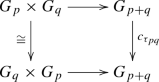
  commute, where $c_{\tau _{pq}}$ denotes conjugation by $\tau _{pq}$. (We do not impose any further conditions upon the $\tau _{pq}$.)

• (4) Injectivity: The multiplication maps are all injective. It follows that the iterated multiplication maps are also injective. Using this, we henceforth regard $G_{p_1}\times \cdots \times G_{p_r}$ as a subgroup of $G_{p_1+\cdots +p_r}$ for each $p_1,\ldots ,p_r\geqslant 0$.

• (5) Intersection: We have

  $$\begin{aligned} (G_{p+q}\times G_r)\cap (G_p\times G_{q+r}) = G_p\times G_q\times G_r, \end{aligned}$$

  for all $p,q,r\geqslant 0$, where $G_{p+q}\times G_r$, $G_p\times G_{q+r}$ and $G_p\times G_q\times G_r$ are all regarded as subgroups of $G_{p+q+r}$.

We denote the neutral element of $G_p$ by $e_p$.

Remark 2.2

We could delete the intersection axiom from Definition 2.1, at the expense of working with the splitting complex of Sect. 6 instead of the splitting poset. See Remark 6.5 for further discussion.

Example 2.3

(Symmetric groups) For $p\geqslant 0$ we let $\Sigma _p$ denote the symmetric group on n letters. Then we may form the family of groups with multiplication $(\Sigma _p)_{p\geqslant 0}$, equipped with the product maps

$$\begin{aligned} \Sigma _p\times \Sigma _q\rightarrow \Sigma _{p+q}, \qquad (f,g)\mapsto f\sqcup g \end{aligned}$$

where $f\sqcup g$ is the automorphism of $\{1,\ldots ,p+q\}\cong \{1,\ldots ,p\}\sqcup \{1,\ldots ,q\}$ given by f on the first summand and by g on the second. Then the axioms of a multiplicative family are all immediately verified. In the case of commutativity, the element $\tau _{pq}$ is the permutation that interchanges the first p and last q letters while preserving their ordering.

Example 2.4

(General linear groups of PIDs) Let R be a PID. For $n\geqslant 0$, let $GL _n(R)$ denote the general linear group of $n\times n$ invertible matrices over R. Then we may form the family of groups with multiplication $( GL _p(R))_{p\geqslant 0}$, equipped with the product maps

$$\begin{aligned} GL _p(R)\times GL _q(R)\rightarrow GL _{p+q}(R), \qquad (A,B)\mapsto \begin{pmatrix} A &{} 0 \\ 0 &{} B \end{pmatrix} \end{aligned}$$

given by the block sum of matrices. The unit, associativity, commutativity, injectivity and intersection axioms all hold by inspection. In the case of commutativity, the element $\tau _{pq}$ is the permutation matrix $=\left( {\begin{matrix} 0 &{} I_q \\ I_p &{} 0 \end{matrix}}\right)$. (It would have been enough to assume that R is an arbitrary ring here. However, as we will see later, we will only be able to apply our results when R is a PID. Indeed, in Proposition 3.4 we will identify the realisation of the splitting poset with Charney’s split building, and this is only possible when R is a PID.)

Example 2.5

(Automorphism groups of free groups) For $p\geqslant 0$ we let $F_p$ denote the free group on p letters, and we let $\mathrm {Aut}(F_p)$ denote the group of automorphisms of $F_p$. Then we may form the family of groups with multiplication $(\mathrm {Aut}(F_p))_{p\geqslant 0}$, equipped with the product maps

$$\begin{aligned} \mathrm {Aut}(F_p)\times \mathrm {Aut}(F_q) \rightarrow \mathrm {Aut}(F_{p+q}), \qquad (f,g)\mapsto f*g. \end{aligned}$$

Here $f*g$ is the automorphism of $F_{p+q}\cong F_p*F_q$ given by f on the first free factor and by g on the second. Then the unit, associativity and commutativity axioms all hold by inspection. In the case of commutativity, the element $\tau _{pq}$ is the automorphism that interchanges the first p generators with the last q generators. The injectivity axiom is also clear. We prove the intersection axiom as follows. Suppose that $f_p*f_{q+r} = f_{p+q}*f_r$ where each $f_\alpha$ lies in $\mathrm {Aut}(F_\alpha )$. We would like to show that $f_{q+r} = f_q*f_r$ for some $f_q\in \mathrm {Aut}(F_q)$. Let $x_i$ be one of the middle q generators. Then $f_{q+r}$ sends $x_i$ to a reduced word in the first $p+q$ generators and to a reduced word in the last $q+r$ generators. Since an element of a free group has a unique reduced expression, it follows that $x_i$ is sent to a word in the middle q generators. Thus $f_{q+r} = f_q*f_r$ for some $f_q:F_q\rightarrow F_q$. By inverting the original equation we see that in fact $f_q\in \mathrm {Aut}(F_q)$.

Example 2.6

(Braid groups) Given $p\geqslant 0$, let $B_p$ denote the braid group on p strands. This is defined to be the group of diffeomorphisms of the disk $D^2$ that preserve the boundary pointwise and that preserve (not necessarily pointwise) a set $X_p\subset D^2$ of p points in the interior of $D^2$, arranged from left to right, all taken modulo isotopies relative to $\partial D^2$ and $X_p$.

The product maps are

$$\begin{aligned} B_p\times B_q\rightarrow B_{p+q}, \qquad (\beta ,\gamma )\mapsto \beta \sqcup \gamma \end{aligned}$$

where $\beta \sqcup \gamma$ denotes the braid obtained by juxtaposing $\beta$ and $\gamma$. More precisely, we choose an embedding $D^2\sqcup D^2\hookrightarrow D^2$ that embeds two copies of $D^2$ ‘side by side’ in $D^2$, in such a way that $X_p\sqcup X_q$ is sent into $X_{p+q}$ preserving the left-to-right order.

Then $\beta \sqcup \gamma$ is defined to be the map given by $\beta$ and $\gamma$ on the respective embedded punctured discs, and by the identity elsewhere. Then the unit, associativity and injectivity axioms are immediate. The commutativity axiom holds when we take $\tau _{pq}$ to be the class of a diffeomorphism that interchanges the two embedded discs, passing the left one above the right. The intersection axiom follows from the fact that we may identify the subgroup $B_p\times B_{q+r}\subseteq B_{p+q+r}$ with the set of isotopy classes of diffeomorphisms that fix an arc that cuts the disc in two, separating the first p punctures from the last $q+r$ punctures, and similarly for $B_{p+q}\times B_r$ and $B_p\times B_q\times B_r$.

Example 2.7

(Mapping class groups) Here we will briefly discuss without proofs one further example that will not be investigated in the present paper.

Let $\Sigma _{g,1}$ denote a surface of genus g with a single boundary component. Let $\Gamma _{g,1}$ denote the mapping class group of diffeomorphisms of $\Sigma _{g,1}$ that fix a neighbourhood of the boundary pointwise, modulo isotopies relative to the boundary. The boundary connect sum operation gives $\Sigma _{g,1}\#_\partial \Sigma _{g',1}\cong \Sigma _{g+g',1}$, and a resulting map $\Gamma _{g,1}\times \Gamma _{g',1}\rightarrow \Gamma _{g+g',1}$. This makes the $\Gamma _{g,1}$ into a family of groups with multiplication.

This family of groups is studied, not as a family with multiplication but as an $E_2$-algebra, by Galatius, Kupers and Randal-Williams in [11]. The associated splitting poset and splitting complex are studied there in detail. See Remarks 3.7 and 4.13.

3 The splitting poset

In this section we define the splitting posets associated to a family of groups with multiplication, and identify them in the case of symmetric groups, braid groups, general linear groups of PIDs, and automorphism groups of free groups. Conditions on the connectivity of these posets are the key assumptions in all of our main theorems.

Definition 3.1

(The splitting poset) Let $(G_p)_{p\geqslant 1}$ be a family of groups with multiplication. Then for $n\geqslant 2$, the nth splitting poset$SP _n$ of $(G_p)_{p\geqslant 1}$ is defined to be the set

$$\begin{aligned} SP _n= \frac{G_n}{G_1\times G_{n-1}} \sqcup \frac{G_n}{G_2\times G_{n-2}} \sqcup \cdots \sqcup \frac{G_n}{G_{n-2}\times G_{2}} \sqcup \frac{G_n}{G_{n-1}\times G_{1}} \end{aligned}$$

equipped with the partial ordering $\leqslant$ with respect to which

$$\begin{aligned} g(G_{p}\times G_{n-p}) \leqslant h(G_q\times G_{n-q}) \end{aligned}$$

if and only if $p\leqslant q$ and there is $k\in G_n$ such that

$$\begin{aligned} g(G_p\times G_{n-p})=k(G_p\times G_{n-p}) \ \text { and }\ h(G_q\times G_{n-q})=k(G_q\times G_{n-q}). \end{aligned}$$

Lemma 3.2 verifies that the relation $\leqslant$ is transitive.

Lemma 3.2

Given an arbitrary chain

$$\begin{aligned} g_0(G_{p_0}\times G_{n-p_0}) \leqslant g_1(G_{p_1}\times G_{n-p_1}) \leqslant \cdots \leqslant g_r(G_{p_r}\times G_{n-p_r}) \end{aligned}$$

(1)

in $SP _n$ we may assume, after possibly choosing new coset representatives, that $g_0=\cdots =g_r$. It follows that $g_i(G_{p_i}\times G_{n-p_i})\leqslant g_j(G_{p_j}\times G_{n-p_j})$ for any $i\leqslant j$.

Proof

We prove by induction on $s=1,2,\ldots ,r$ that given an arbitrary chain (1) we may assume, after choosing new coset representatives, that $g_0=\cdots =g_s=g$ for some $g\in G_n$, the case $s=r$ being our desired result.

When $s=1$, the claim is immediate from the definition of $\leqslant$.

For the induction step, suppose that the claim holds for s. Take an arbitrary chain (1) and use the induction hypothesis to choose new coset representatives so that $g_0=\cdots =g_s=g$. Since $g(G_{p_s}\times G_{n-p_s})\leqslant g_{s+1}(G_{p_{s+1}}\times G_{n-p_{s+1}})$ we may assume, after replacing $g_{s+1}$ if necessary, that $g (G_{p_s}\times G_{n-p_s})=g_{s+1}(G_{p_s}\times G_{n-p_s})$. Then there are $\gamma \in G_{p_s}$ and $\delta \in G_{n-p_s}$ such that $g^{-1}g_{s+1}=\gamma \oplus \delta$. Since $e_{p_s}\oplus \delta$ lies in $G_{p_t}\times G_{n-p_t}$ for $t\leqslant s$, we may replace g with $g(e_{p_s}\oplus \delta )$. And since $\gamma \oplus e_{n-p_s}$ lies in $G_{p_{s+1}}\times G_{n-p_{s+1}}$, we may replace $g_{s+1}$ with $g_{s+1}(\gamma ^{-1}\oplus e_{n-p_s})$. But then $g_{s+1}=g$. So $g_0=\cdots =g_{s+1}$ as required. $\square$

Now we will identify the splitting posets associated to the symmetric groups, general linear groups of PIDs, automorphism groups of free groups, and braid groups.

Proposition 3.3

(Splitting posets for symmetric groups) For the family of groups with multiplication $(\Sigma _p)_{p\geqslant 0}$, the nth splitting poset $SP _n$ is isomorphic to the poset of proper subsets of $\{1,\ldots ,n\}$ under inclusion.

Proof

We define a bijection $\phi$ from $SP _n$ to the poset of proper subsets of $\{1,\ldots ,n\}$ by the rule

$$\begin{aligned} \phi \left( g(\Sigma _p\times \Sigma _{n-p}) \right) = \{g(1),\ldots ,g(p)\}. \end{aligned}$$

This $\phi$ is a well-defined bijection, and we must show that

$$\begin{aligned} g(\Sigma _p\times \Sigma _{n-p})\leqslant h(\Sigma _q\times \Sigma _{n-q}) \iff \{g(1),\ldots ,g(p)\}\subseteq \{h(1),\ldots ,h(q)\}. \end{aligned}$$

If the first condition holds then $p\leqslant q$ and we may assume that $g=h$, so that the second condition follows immediately. If the second condition holds then $p\leqslant q$ and, replacing h by $h\circ (k\times \mathrm {Id})$ and g by $g\circ (\mathrm {Id}\times l)$ for an appropriate $k\in \Sigma _q$ and $l\in \Sigma _{n-p}$, we may assume that $g=h$, so that the first condition holds. $\square$

Let R be a PID. To identify the splitting posets associated to the family $( GL _p(R))_{p\geqslant 0}$, recall that Charney in [4] defined $S_R(R^n)$ to be the poset of ordered pairs (P, Q) of proper submodules of $R^n$ satisfying $P\oplus Q=R^n$, equipped with the partial order $\leqslant$ defined by

$$\begin{aligned} (P,Q)\leqslant (P',Q') \iff P\subseteq P'\text { and }Q\supseteq Q'. \end{aligned}$$

Charney then defined the split building of $R^n$, denoted by $[R^n]$, to be the realisation $|S_R(R^n)|$. (Note that Charney worked with arbitrary Dedekind domains. We work with PIDs only in order to relate the splitting poset with the split building. We do not know what happens to the connectivity of $| SP _n|$ in the case that R is not a PID.)

Proposition 3.4

(Splitting posets for general linear groups of PIDs) Let R be a PID. For the family of groups with multiplication $( GL _n(R))_{n\geqslant 0}$, the splitting poset $SP _n$ is isomorphic to $S_R(R^n)$, so that $| SP _n|$ is isomorphic to the split building $[R^n]$.

Proof

Define $s_1,\ldots ,s_{n-1}\in SP _n$ and $t_1,\ldots ,t_{n-1}\in S_R(R^n)$ by

$$\begin{aligned} s_p=e_n( GL _p(R)\times GL _{n-p}(R)), \qquad t_p=(\mathrm {span}(x_1,\ldots ,x_p),\mathrm {span}(x_{p+1},\ldots ,x_n)), \end{aligned}$$

where $e_n\in GL _n(R)$ denotes the identity element and $x_1,\ldots ,x_n$ is the standard basis of $R^n$. Then the following three properties hold for the elements $s_i\in SP _n$, and their analogues hold for the $t_i\in S_R(R^n)$.

• (1) $s_1,\ldots ,s_{n-1}$ are a complete set of orbit representatives for the $GL _n(R)$ action on $SP _n$.

• (2) The stabiliser of $s_p$ is $GL _p(R)\times GL _{n-p}(R)$.

• (3) $x\leqslant y$ if and only if there is $g\in GL _n(R)$ such that $x=g\cdot s_p$ and $y=g\cdot s_q$ where $p\leqslant q$.

It follows immediately that there is a unique isomorphism of posets $SP _n\rightarrow S_R(R^n)$ satisfying $s_i\mapsto t_i$ for all i.

The three properties hold for $s_i\in SP _n$ by definition. We prove them for $t_i\in S_R(R^n)$ as follows. For (1), the fact that R is a PID guarantees that if $(P,Q)\in S_R(R^n)$ then P and Q are free, of ranks p and q say, such that $p+q=n$. If we choose bases of P and Q and concatenate them to form an element $A\in GL _n(R)$, then $A\cdot t_p = (P,Q)$ as required. Property (2) is immediate. For (3), suppose that $(P,Q)\leqslant (P',Q')$ and let $p=\mathrm {rank}(P)$ and $p'=\mathrm {rank}(P')$, so that $p\leqslant p'$. Then

$$\begin{aligned} R^n = P\oplus (P'\cap Q)\oplus Q', \qquad P\oplus (P'\cap Q) = P', \qquad (P'\cap Q)\oplus Q' = Q. \end{aligned}$$

Let g denote the element of $GL _n(R)$ whose columns are given by a basis of P, followed by a basis of $(P'\cap Q)$, followed by a basis of $Q'$. Again this is possible since R is a PID. Then $(P,Q)=g\cdot t_p$ and $(P',Q')=g\cdot t_{p'}$ where $p\leqslant p'$, as required. $\square$

Let us now identify the splitting posets for automorphism groups of free groups. The situation is closely analogous to that for general linear groups. Define $S(F_n)$, for each $n\geqslant 2$, to be the poset of ordered pairs (P, Q) of proper subgroups of $F_n$ satisfying $P*Q = F_n$. It is equipped with the partial order under which $(P,Q)\leqslant (P',Q')$ if and only if $(P,Q)=(J_0,J_1*J_2)$ and $(P',Q')=(J_0*J_1,J_2)$ for some proper subgroups $J_0,J_1,J_2$ of $F_n$ satisfying $J_0*J_1*J_2 = F_n$. (Note that the condition in the definition of $\leqslant$ is stronger than assuming that $P\subseteq P'$ and $Q'\supseteq Q$). The proof of the following proposition is similar to that of Proposition 3.4, and we leave the details to the reader.

Proposition 3.5

(Splitting posets for automorphism groups of free groups) For the family of groups with multiplication $(\mathrm {Aut}(F_n))_{n\geqslant 0}$, the splitting poset $SP _n$ is isomorphic to $S(F_n)$.

Let us now identify the splitting posets associated to the family $(B_p)_{p\geqslant 0}$ of braid groups. See Example 2.6 for the relevant notation. Given $n\geqslant 2$, let us define a poset as follows. The elements of are the arcs embedded in $D^2{\setminus } X_n$, starting at the ‘north pole’ of the disc and ending at the ‘south pole’, such that $X_n$ meets both components of their complement, all taken modulo isotopies in $D^2{\setminus } X_n$ that preserve the endpoints.

Given , we say that $\alpha \leqslant \beta$ if $\alpha$ and $\beta$ have representatives a and b that meet only at their endpoints, and such that a lies ‘to the left’ of b. (More precisely, a and b must meet the north pole in anticlockwise order and the south pole in clockwise order).

Again, the proof of the following is similar to that of Proposition 3.4, and we leave the details to the reader.

Proposition 3.6

(Splitting posets for braid groups) For the family of groups with multiplication $(B_p)_{p\geqslant 0}$, we have .

Remark 3.7

(Mapping class groups) As mentioned in Example 2.7, Galatius, Kupers and Randal-Williams [11] have studied the mapping class groups $\Gamma _{g,1}$ of isotopy classes of diffeomorphisms of $\Sigma _{g,1}$ that fix the boundary pointwise using the techniques discussed in Sect. 1.2. They identify the resulting splitting poset with a poset of arcs travelling between distinct marked points on the boundary of $\Sigma$, much as we have done in Proposition 3.6. See Sections 3 and 4 of [11], especially Definition 3.3, Proposition 4.4 and Definition 4.5.

4 Examples of connectivity of $| SP _n|$

Our Theorems A, B and C apply to a family of groups with multiplication only when the associated splitting posets satisfy the connectivity condition that each $| SP _n|$ is $(n-3)$-connected. In this section we verify this condition for our main examples: symmetric groups, where the result is elementary; general linear groups of PIDs, where the result was proved by Charney in [4]; automorphism groups of free groups, where we make use of Hatcher and Vogtmann’s result on the connectivity of the poset of free factorisations of$F_n$ in [15]; and for braid groups, where the claim is a variant of known results on arc complexes.

Let us fix our definitions and notation for realisations of posets. If P is a poset, then its order complex (or flag complex or derived complex) $\Delta (P)$ is the abstract simplicial complex whose vertices are the elements of P, and in which vertices $p_0,\ldots ,p_r$ span an r-simplex if they form a chain $p_0<\cdots <p_r$ after possibly reordering. The realisation |P| of P is then defined to be the realisation $|\Delta (P)|$ of $\Delta (P)$. We will usually not distinguish between a simplicial complex and its realisation. So if P is a poset, then the simplicial complex $\Delta (P)$ and topological space $|\Delta (P)|$ will both be denoted by |P|. When we discuss topological properties of a poset or of a simplicial complex, we are referring to the topological properties of its realisation as a topological space.

4.1 Symmetric groups

The result for symmetric groups is elementary.

Proposition 4.1

(Connectivity of $| SP _n|$ for symmetric groups) For the family of groups with multiplication $(\Sigma _p)_{p\geqslant 0}$ we have $| SP _n|\cong S^{n-2}$, and in particular $| SP _n|$ is $(n-3)$-connected.

Proof

Let $\partial \Delta ^{n-1}$ denote the simplicial complex given by the boundary of the simplex with vertices $1,\ldots ,n$. Then the face poset of $\partial \Delta ^{n-1}$ is exactly the poset of proper subsets of $\{1,\ldots ,n\}$ ordered by inclusion. But we saw in Proposition 3.3 that the latter is isomorphic to $SP _n$. Thus as required.

4.2 General linear groups of PIDs

Let R be a PID. In Proposition 3.4 we saw that for the family of groups with multiplication $( GL _p(R))_{p\geqslant 0}$ there is an isomorphism $SP _n\cong S_R(R^n)$, where $S_R(R^n)$ is the poset whose realisation is the split building $[R^n]$. Since R is in particular a Dedekind domain, Theorem 1.1 of [4] shows that $[R^n]$ has the homotopy type of a wedge of $(n-2)$-spheres. So we immediately obtain the following.

Proposition 4.2

(Connectivity of $| SP _n|$ for general linear groups of PIDs) Let R be a PID. For the family of groups with multiplication $( GL _p(R))_{p\geqslant 0}$, and for any $n\geqslant 2$, $| SP _n|$ has the homotopy type of a wedge of $(n-2)$-spheres, and in particular is $(n-3)$-connected.

4.3 Automorphism groups of free groups

Now we give the proof of the connectivity condition on the splitting posets for automorphism groups of free groups. This is the most involved of our connectivity proofs.

Definition 4.3

Let F be a free group of finite rank. Define P(F) to be the poset of ordered tuples $H=(H_0,\ldots ,H_r)$ of proper subgroups of F such that $r\geqslant 1$ and $H_0*\cdots *H_r=F$. It is equipped with the partial order in which $H\geqslant K$ if K can be obtained by repeatedly amalgamating adjacent entries of H.

Theorem 4.4

If F has rank n, then |P(F)| has the homotopy type of a wedge of $(n-2)$-spheres.

Corollary 4.5

(Connectivity of $| SP _n|$ for automorphism groups of free groups) For the family of groups with multiplication $(\mathrm {Aut}(F_p))_{p\geqslant 0}$, the splitting poset $| SP _n|$ has the homotopy type of a wedge of $(n-2)$-spheres, and in particular is $(n-3)$-connected.

This result has been obtained independently, and with the same proof, as part of work in progress by Kupers, Galatius and Randal-Williams.

Proof of Corollary 4.5

If P is a poset then we denote by $P'$ the derived poset of chains $p_0<\cdots <p_r$ in P ordered by inclusion. This is the same thing as the face poset of $\Delta (P)$, and its realisation satisfies $|P'|\cong |P|$.

Recall from Proposition 3.5 that $SP _n$ is isomorphic to the poset $S(F_n)$ defined there. So it will suffice to show that $P(F_n)$ is isomorphic to $S(F_n)'$, for then $| SP _n|\cong |S(F_n)|\cong |S(F_n)'|\cong |P(F_n)|$ and the result follows from Theorem 4.4. Consider the maps

$$\begin{aligned} \lambda :P(F_n)\rightarrow S(F_n)', \qquad \mu :S(F_n)'\rightarrow P(F_n) \end{aligned}$$

defined by

$$\begin{aligned} \lambda \Bigl (H_0,\ldots ,H_{r+1}\Bigr )= \Bigl [ (H_0,H_1*\cdots *H_{r+1})<\cdots < (H_0*\cdots *H_{r},H_{r+1})\Bigr ] \end{aligned}$$

and

$$\begin{aligned} \mu \Bigl [ (A_0,B_0)<\cdots < (A_r,B_r)\Bigr ] = \Bigl (A_0,A_1\cap B_0,A_2\cap B_1, \ldots ,A_r\cap B_{r-1},B_r\Bigr ). \end{aligned}$$

Then one can verify that $\lambda$ and $\mu$ are mutually inverse maps of posets. The verification requires one to use the fact that if $(X_1,Y_1)<(X_2,Y_2)<(X_3,Y_3)$, then $X_{1}*(X_2\cap Y_{1})=X_2$, $Y_{2}*(Y_1\cap X_{2})=Y_1$ and $(X_2\cap Y_{1})*(X_{3}\cap Y_2)=X_{3}\cap Y_{1}$, which follow from the definition of the partial ordering on $S(F_n)$. $\square$

We now move towards the proof of Theorem 4.4. In order to do so we require another definition.

Definition 4.6

Let F be a free group of finite rank. Define Q(F) to be the poset of unordered tuples $H=\{H_0,\ldots ,H_r\}$ of proper subgroups of F such that $r\geqslant 1$ and $H_0*\cdots *H_r=F$. Give it the partial order in which $H\geqslant K$ if K can be obtained by repeatedly amalgamating entries of H, adjacent or otherwise. Let $f:P(F)\rightarrow Q(F)$ denote the map that sends an ordered tuple to the same tuple, now unordered.

The poset $Q(F_n)$ is exactly the opposite of the poset of free factorisations of$F_n$. This poset was introduced and studied by Hatcher and Vogtmann in Section 6 of [15], where it was shown that its realisation has the homotopy type of a wedge of $(n-2)$-spheres. It follows that if F is a free group of rank n then |Q(F)| has the homotopy type of a wedge of $(n-2)$-spheres.

We will now prove Theorem 4.4 by deducing the connectivity of |P(F)| from the known connectivity of |Q(F)|. In order to do this we will use a poset fibre theorem due to Björner, Wachs and Welker [2]. Let us recall some necessary notation. Given a poset P and an element $p\in P$, we define $P_{<p}$ to be the poset $\{q\in P\mid q<p\}$. We define $P_{\leqslant p}$, $P_{>p}$ and $P_{\geqslant p}$ similarly. The length$\ell (P)$ of a poset P is defined to be the maximum $\ell$ such that there is a chain $p_0<p_1<\cdots <p_\ell$ in P, and is defined to be $\infty$ otherwise. The length of the empty poset is defined to be $-1$. We let $*$ denote the join of topological spaces.

Theorem 4.7

(Bjorner–Wachs–Welker [2]) Let P and Q be posets where $\ell (Q_{\leqslant q})<\infty$ for all $q\in Q$. Let $f:P\rightarrow Q$ be a map of posets such that for all $q\in Q$ the fibre $|f^{-1}(Q_{\leqslant q})|$ is $\ell (f^{-1}(Q_{<q}))$-connected. Then so long as |Q| is connected, we have

$$\begin{aligned} |P|\simeq |Q|\vee \bigvee _{q\in Q} |f^{-1}(Q_{\leqslant q})|*|Q_{>q}|. \end{aligned}$$

This result appears as Theorem 1.1 of [2], under the additional assumption that P and Q are finite. However, the same proof applies to give the more general statement where P is arbitrary and $\ell (Q_{\leqslant q})<\infty$ for all $q\in Q$, so long as one chases the references far enough to see that the stronger assumptions are not required. Let us explain in detail. The proof of [2, Theorem 1.1] requires the use of [2, Theorem 2.5], but does not require any finiteness assumptions beyond that. So it is enough to explain why [2, Theorem 2.5], which is only stated for P and Q finite, in fact applies to arbitrary P and to Q with $\ell (Q)<\infty$. The proof of [2, Theorem 2.5] requires the finiteness assumptions only in the following places:

• The proof relies on the notion of arrangement of subspaces and the associated result [2, Corollary 2.4]. Such an arrangement is defined to be a finite collection of subspaces, and [2, Corollary 2.4] is only stated under that assumption. However, one may instead define an arrangement of subspaces to be a possibly-infinite collection that forms a poset satisfying for all . Then one may re-prove [2, Corollary 2.4] in this generality by referring not to [2, Lemma 2.3] but instead to [1, Proposition 6.9]. The latter is again only stated for finite posets, but [1, Remark 6.10] explains that it also holds for posets of finite length.

• The arrangement of subspaces appearing in the proof is indexed by Q, so with the generalisation in the above bullet point, this aspect of the proof holds under the assumption that $\ell (Q_{\leqslant q})<\infty$ for all $q\in Q$.

• The proof also relies on [2, Lemma 2.2], which is only stated for finite posets. But that is a restatement of [31, Lemma 4.9], which is in fact stated for arbitrary posets.

• Finally, the proof uses [2, Lemma 2.1], which is a restatement of [31, Lemma 4.6], which is stated for arbitrary posets.

In conclusion, Theorem 4.7 holds in the stated generality.

Proof of Theorem 4.4

The proof is by induction on the rank of F. When ${{\,\mathrm{rank}\,}}(F)=2$ we need only observe that P(F) is an infinite set with trivial partial order, so that |P(F)| is an infinite discrete set, and in particular is a wedge of 0-spheres. Suppose now that ${{\,\mathrm{rank}\,}}(F)\geqslant 3$ and that the claim holds for all free groups of smaller rank than F. We consider the map $f:P(F)\rightarrow Q(F)$ that forgets the ordering of tuples. Since ${{\,\mathrm{rank}\,}}(F)\geqslant 3$, |Q(F)| is connected. Suppose that $H=\{H_0,\ldots ,H_{r}\}\in Q(F)$. Then Lemmas 4.8, 4.9, 4.10 and 4.11 tell us the following.

• $\ell (f^{-1}(Q(F)_{<H}))=r-2$

• $|f^{-1}(Q(F)_{\leqslant H})|\cong S^{r-1}$

• $|Q(F)_{>H}|\simeq \bigvee S^{n-r-2}$

Since $S^{r-1}$ is $(r-2)$-connected, and since $\ell (Q(F)_{\leqslant \{H_0,\ldots ,H_{r}\}})=(r-1)<\infty$ for all $\{H_0,\ldots ,H_{r}\}\in Q(F)$, we may apply apply Theorem 4.7, which tells us that

$$\begin{aligned} |P(F)|&\simeq |Q(F)|\vee \bigvee _{H\in Q(F)} \bigl (|f^{-1}(Q(F)_{\leqslant H})|*|Q(F)_{>H}|\bigr ).\\&\simeq \bigvee S^{n-2} \vee \bigvee _{H\in Q(F)} \left( \left( \bigvee S^{n-r-2}\right) *S^{r-1}\right) \\&\simeq \bigvee S^{n-2} \vee \bigvee _{H\in Q(F)}\bigvee \left( S^{n-r-2}*S^{r-1}\right) \\&\simeq \bigvee S^{n-2}\vee \bigvee _{H\in Q(F)}\bigvee S^{n-2}\\&\simeq \bigvee S^{n-2} \end{aligned}$$

as required. $\square$

Lemma 4.8

Let F be a free group of finite rank and let $H=\{H_0,\ldots ,H_r\}\in Q(F)$. Then $\ell (f^{-1}(Q(F)_{<H}))=r-2$.

Proof

After fixing an ordering of the tuple H, one can amalgamate $(r-1)$ adjacent entries before obtaining a 2-tuple. This shows that $\ell (f^{-1}(Q(F)_{\leqslant H}))=r-1$. Since any maximal chain must include H itself (with some ordering) it follows that $\ell (f^{-1}(Q(F)_{<H}))=r-2$. $\square$

Lemma 4.9

Let F be a free group of finite rank and let $H=\{H_0,\ldots ,H_r\}\in Q(F)$. Then $|f^{-1}(Q(F)_{\leqslant H})|\cong S^{r-1}$.

Proof

The poset $f^{-1}(Q(F)_{\leqslant H})$ is the subposet of P(F) consisting of tuples $K=(K_0,\ldots ,K_s)$ where each $K_j$ is an amalgamation of some of the $H_i$. It is isomorphic to the poset $X_r$ of sequences $F=(F_0\subset F_1\subset \cdots \subset F_{s-1})$ of proper subsets of $\{0,\ldots , r\}$, where $F'\leqslant F$ if $F'$ can be obtained from F by forgetting terms of the sequence. The isomorphism

$$\begin{aligned} X_r\xrightarrow {\ \cong \ }f^{-1}(Q(F)_{\leqslant H}) \end{aligned}$$

sends $F=(F_0\subset \cdots \subset F_{s-1})$ to $K=(K_0,\ldots , K_s)$ where for $i\leqslant s-1$, $K_j$ is the subgroup generated by the $H_i$ for $i\in F_j{\setminus } F_{j-1}$, and where $K_s$ is the subgroup generated by the $H_j$ for $j\not \in F_{s-1}$. Now $X_n$ is isomorphic to the poset of faces of the barycentric subdivision of $\partial \Delta ^r$, as we see by identifying $F_0\subset \cdots \subset F_{s-1}$ with the face whose vertices are the barycentres of the simplices spanned by the $F_i$. So $|X_n|\cong \partial \Delta ^r\cong S^{r-1}$ as claimed. $\square$

Lemma 4.10

Let F be a free group of finite rank and let $H=\{H_0,\ldots ,H_r\}\in Q(F)$. Then

$$\begin{aligned} |Q(F)_{> H}| \cong |Q(H_0)|*\cdots *|Q(H_r)|. \end{aligned}$$

Proof

Given a poset P, let CP denote the poset obtained by adding a new minimal element 0. There is an isomorphism

$$\begin{aligned} Q(F)_{\geqslant H} \cong CQ(H_0)\times \cdots \times CQ(H_r). \end{aligned}$$

It simply takes a tuple $K=\{K_0,\ldots ,K_s\}$ and sends it to the element of $CQ(H_0)\times \cdots \times CQ(H_r)$ whose $CQ(H_i)$-component is the tuple consisting of those $K_j$ which are contained in $H_i$ if there are more than one such, and which is 0 otherwise, in which case $H_i$ itself appears as one of the $K_j$. This isomorphism identifies H itself with the tuple $(0,\ldots ,0)$, so that we obtain a restricted isomorphism

$$\begin{aligned} Q(F)_{> H} \cong CQ(H_0)\times \cdots \times CQ(H_r){\setminus }(0,\ldots ,0). \end{aligned}$$

Now the realisation of the right hand side is exactly $|Q(H_0)|*\cdots *|Q(H_r)|$ (see Proposition 1.9 of [23] for instance), and so the result follows. $\square$

Lemma 4.11

Let F be a free group of finite rank and let $H=(H_0,\ldots ,H_r)\in Q(F)$. Then $|Q(H_0)|*\cdots *|Q(H_r)|$ has the homotopy type of a wedge of $(n-r-2)$-spheres.

Proof

Write $s_i$ for the rank of $H_i$, so that $|Q(H_i)|$ has the homotopy type of a wedge of $(s_i-2)$-spheres. Since wedge sums commute with joins up to homotopy equivalence, it follows that $|Q(H_0)|*\cdots *|Q(H_r)|$ has the homotopy type of a wedge of copies of $S^{s_0-2}*\cdots *S^{s_r-2}$. But then

$$\begin{aligned} S^{s_0-2}*\cdots *S^{s_r-2} \cong S^{(s_0-2)+\cdots +(s_r-2)+r} =S^{(s_0+\cdots +s_r)-2(r+1) +r} =S^{n -r-2} \end{aligned}$$

as required. $\square$

4.4 Braid groups

Now we investige the connectivity of the realisations of the splitting posets for braid groups. In this case we will appeal to well-known connectivity results for complexes of arcs.

Proposition 4.12

(Connectivity of $| SP _n|$ for braid groups) For the family of groups with multiplication $(B_p)_{p\geqslant 0}$, and for any $n\geqslant 2$, $| SP _n|$ has the homotopy type of a wedge of $(n-2)$-spheres, and in particular is $(n-3)$-connected.

Proof

Recall from Proposition 3.5 that we identified $SP _n$ with the poset of arcs defined there. Thus is (the realisation of) the simplicial complex with vertices the elements of , in which vertices $\alpha _0,\ldots ,\alpha _r$ span a simplex if and only if, after possibly reordering, $\alpha _0<\cdots < \alpha _r$. Now $\alpha _0<\cdots < \alpha _r$ holds if and only if the $\alpha _i$ have representatives $a_i$ that are disjoint except at their endpoints, and such that $a_0,\ldots ,a_r$ meet the north pole in anticlockwise order. Thus is the realisation of the simplicial complex whose vertices are isotopy classes of nontrivial (they do not separate a disc from the remainder of the surface) arcs in $D^2{\setminus } X_n$ from the north pole to the south, where a collection of vertices form a simplex if they have representing arcs that can be embedded disjointly except at their endpoints. In the notation of Section 4 of [30], this is exactly the complex where $S=D^2{\setminus } X_n$, $\Delta _0\subset \partial D^2$ is the set containing just the north pole, and $\Delta _1\subset \partial D^2$ is the set containing just the south pole. Now, replacing S with the complement of n open discs in $D^2$ does not change the isomorphism type of the complex. But in that case, Lemma 4.7 of [30] applies to show that has connectivity $(n-2)$ greater than that of , which is $(-1)$-connected since it is a simply a nonempty set. $\square$

Remark 4.13

(Mapping class groups) In Example 2.7 and Remark 3.7 we mentioned that in [11], Galatius, Kupers and Randal-Williams introduce a splitting poset (and splitting complex) for the mapping class groups $\Gamma _{g,1}$. Theorem 3.4 of their paper shows that it is $(n-3)$-connected, as with the complexes appearing here. Comparing that result, which holds for surfaces with arbitrary genus and no marked points, with Proposition 4.12, which holds for surfaces of genus 0 with arbitrarily many marked points, we expect that these results generalise to the case of surfaces with marked points and arbitrary genus.

5 Proofs of the applications

In this section we will assume that Theorems A, B and C hold, and we will prove the remaining theorems stated in the introduction. We begin with three closely analogous lemmas about the groups $GL _n(\mathbb {Z})$, $GL _n(\mathbb {F}_2)$ and $\mathrm {Aut}(F_n)$.

Lemma 5.1

Define elements of $GL _n(\mathbb {Z})$, $n=1,2,3$ as follows

$$\begin{aligned} s_1=\begin{pmatrix} -1 \end{pmatrix}, \qquad s_2=\begin{pmatrix} -1 &{} \\ &{} 1 \end{pmatrix}, \qquad s_3=\begin{pmatrix} -1 &{} &{} \\ &{} 1 &{} \\ &{} &{} 1\end{pmatrix}, \qquad t=\begin{pmatrix} 1 &{} 1 \\ 0 &{} 1\end{pmatrix}. \end{aligned}$$

Use the same symbols to denote the corresponding elements of $H_1( GL _n(\mathbb {Z});\mathbb {Z}) = GL _n(\mathbb {Z})_\mathrm {ab}$. Then $H_1( GL _1(\mathbb {Z});\mathbb {Z})$, $H_1( GL _2(\mathbb {Z});\mathbb {Z})$ and $H_1( GL _3(\mathbb {Z});\mathbb {Z})$ are elementary abelian 2-groups with generators $s_1\in H_1( GL _1(\mathbb {Z});\mathbb {Z})$, $s_2,t\in H_1( GL _2(\mathbb {Z});\mathbb {Z})$ and $s_3\in H_1( GL _3(\mathbb {Z});\mathbb {Z})$. The stabilisation maps have the following effect.

Proof

There are split extensions

$$\begin{aligned} SL _n(\mathbb {Z})\longrightarrow GL _n(\mathbb {Z})\xrightarrow {\det }\{\pm 1\} \end{aligned}$$

with section determined by $-1\mapsto s_n$, so that we have isomorphisms

$$\begin{aligned} H_1( GL _n(\mathbb {Z});\mathbb {Z})\cong H_1( SL _n(\mathbb {Z});\mathbb {Z})_{\{\pm 1\}}\oplus \mathbb {Z}/2\mathbb {Z}, \end{aligned}$$

where $\mathbb {Z}/2\mathbb {Z}$ is generated by the class of $s_n$. This isomorphism respects the stabilisation maps. Now $H_1( SL _1(\mathbb {Z});\mathbb {Z})$ obviously vanishes, and $H_1( SL _3(\mathbb {Z});\mathbb {Z})$ vanishes since $SL _n(\mathbb {Z})$ is perfect for $n\geqslant 3$. So it suffices to show that $H_1( SL _2(\mathbb {Z});\mathbb {Z})_{\{\pm 1\}}$ is a group of order 2 generated by t.

Let us write

$$\begin{aligned} u=\begin{pmatrix} 0 &{} -1 \\ 1 &{} 1 \end{pmatrix}, \qquad v=\begin{pmatrix} 0 &{} 1 \\ -1 &{} 0\end{pmatrix}. \end{aligned}$$

Then $H_1( SL _2(\mathbb {Z});\mathbb {Z})\cong \mathbb {Z}/12\mathbb {Z}$, where $v\leftrightarrow 3$ and $u\leftrightarrow 2$ [19, p.91]. One can verify that $s_2vs_2^{-1}=v^{-1}$ and $s_2us_2^{-1}=v^{-1}u^{-1}v$, so that $\{\pm 1\}$ acts on $H_1( SL _2(\mathbb {Z}))$ by negation. Consequently $H_1( SL _2(\mathbb {Z});\mathbb {Z})_{\{\pm 1\}}=(\mathbb {Z}/12\mathbb {Z})_{\{\pm 1\}}$ has order 2 with generator $t=vu$ as required. $\square$

Lemma 5.2

$H_1( GL _n(\mathbb {F}_2)) = GL _n(\mathbb {F}_2)_\mathrm {ab}$ is trivial for $n=1,3$, and is generated by the element t determined by the matrix $\left( {\begin{matrix} 1 &{} 1 \\ 0 &{} 1\end{matrix}}\right)$ for $n=2$.

Proof

For $n=1$ this is trivial, and for $n=3$ it follows from the fact that $GL _3(\mathbb {F}_2)= SL _3(\mathbb {F}_2)$ is perfect. For $n=2$, we simply observe that $GL _2(\mathbb {F}_2)$ is a dihedral group of order 6 generated by the involutions

$$\begin{aligned} \begin{pmatrix} 1 &{} 1 \\ 0 &{} 1\end{pmatrix} \quad \text {and}\quad \begin{pmatrix} 0 &{} 1 \\ 1 &{} 0\end{pmatrix}, \end{aligned}$$

so that the abelianization is a group of order 2 generated by either of the involutions. $\square$

Lemma 5.3

Define elements of $\mathrm {Aut}(F_n)$, $n=1,2,3$ as follows. For $n=1,2,3$ let $s_i$ denote the transformation that inverts the first letter and fixes the others. And let $t\in \mathrm {Aut}(F_2)$ denote the transformation $x_1\mapsto x_1$, $x_2\mapsto x_1x_2$. Use the same symbols to denote the corresponding elements of $H_1(\mathrm {Aut}(F_n);\mathbb {Z}) = Aut(F_n)_\mathrm {ab}$. Then $H_1(\mathrm {Aut}(F_1);\mathbb {Z})$, $H_1(\mathrm {Aut}(F_2);\mathbb {Z})$ and $H_1(\mathrm {Aut}(F_3);\mathbb {Z})$ are elementary abelian 2-groups with generators $s_1\in H_1(\mathrm {Aut}(F_1);\mathbb {Z})$, $s_2,t\in H_1(\mathrm {Aut}(F_2);\mathbb {Z})$ and $s_3\in H_1(\mathrm {Aut}(F_3);\mathbb {Z})$. The stabilisation maps have the following effect.

Proof

We claim that the linearisation map $\mathrm {Aut}(F_n)\rightarrow GL _n(\mathbb {Z})$ is an isomorphism on abelianisations for all n. Since the linearisation map sends the generators $s_1,s_2,s_3,t$ listed here to the corresponding generators from Lemma 5.1, the result then follows from Lemma 5.1. It remains to prove the claim.

In the case $n=1$ the claim holds because the linearisation map map itself is an isomorphism.

In the case $n=2$ the claim holds because the map $\mathrm {Out}(F_2)\rightarrow GL _2(\mathbb {Z})$ is an isomorphism (see Theorem 2.3.4 of [6] and the references there) so there is an extension $F_2\rightarrow \mathrm {Aut}(F_2)\rightarrow GL _2(\mathbb {Z})$ of groups, and a corresponding exact sequence

$$\begin{aligned} ((F_2)_\mathrm {ab})_{ GL _2(\mathbb {Z})} \rightarrow \mathrm {Aut}(F_2)_\mathrm {ab} \rightarrow GL _2(\mathbb {Z})_\mathrm {ab} \rightarrow 0 \end{aligned}$$

where $((F_2)_\mathrm {ab})_{ GL _2(\mathbb {Z})}$ denotes the coinvariants of $(F_2)_\mathrm {ab}$ with respect to the $GL _2(\mathbb {Z})$-action. (The existence of this exact sequence follows for example from the Lyndon–Hochschild–Serre spectral sequence.) Now the action of $GL _2(\mathbb {Z})$ on $(F_2)_\mathrm {ab}=\mathbb {Z}^2$ is the tautological one, so that the coinvariants $((F_2)_\mathrm {ab})_{ GL _2(\mathbb {Z})}$ vanish, and the claim follows in this case.

For $n\geqslant 3$ the claim holds because $SL _n(\mathbb {Z})$ is perfect, as is the subgroup $SA_n$ of $\mathrm {Aut}(F_n)$ consisting of automorphisms with determinant one. (For the last claim we refer to the presentation of $SA_n$ given in Theorem 2.8 of [13]).

Proof of Theorem F

Let $\mathbb {F}$ be a field of characteristic 2. We will use the Künneth isomorphism $H_1(-;\mathbb {F})\cong H_1(-;\mathbb {Z})\otimes \mathbb {F}$ without further mention, and in this proof all homology groups will be taken with coefficients in $\mathbb {F}$. We will use the fact that the stabilisation map $s_*$ is induced by multiplication with the neutral element of $GL _1(\mathbb {Z})$. Thus, if we let $\sigma \in H_0( GL _1(\mathbb {Z}))$ be the class of a point, then $s_*(y) = \sigma \cdot y$ for any $y\in GL _n(\mathbb {Z})$.

Theorem B states that the kernel of the map

$$\begin{aligned} s_*:H_m( GL _{2m}(\mathbb {Z})) \twoheadrightarrow H_m( GL _{2m+1}(\mathbb {Z})) \end{aligned}$$

(2)

is the image of the product map

$$\begin{aligned} H_{1}( GL _{2}(\mathbb {Z}))^{\otimes {m-1}} \otimes \ker [H_1( GL _2(\mathbb {Z}))\xrightarrow {s_*} H_1( GL _3(\mathbb {Z}))] \longrightarrow H_{m}( GL _{2m}(\mathbb {Z})). \end{aligned}$$

(3)

By Lemma 5.1, $H_1( GL _2(\mathbb {Z}))$ is spanned by the classes $s_2$ and t, and the kernel of $s_*:H_1( GL _2(\mathbb {Z}))\rightarrow H_1( GL _3(\mathbb {Z}))$ is spanned by t, so that (3) becomes

$$\begin{aligned} \mathrm {span}\{s_2,t\}^{\otimes m-1}\otimes \mathrm {span}\{t\} \longrightarrow H_{m}( GL _{2m}(\mathbb {Z})). \end{aligned}$$

However, any product involving both $s_2$ and t vanishes, since

$$\begin{aligned} s_2\cdot t = s_*(s_1)\cdot t = (\sigma \cdot s_1)\cdot t = s_1\cdot (\sigma \cdot t) = s_1\cdot s_*(t) = s_1\cdot 0 = 0. \end{aligned}$$

Here we have used associativity and commutativity of the product. So it follows that the image of the product map (3) is precisely the span of $t^m$, which gives us the claimed description of of kernel of (2).

Next, Theorem C states that the map

$$\begin{aligned} H_m( GL _{2m-1}(\mathbb {Z}))\oplus H_1( GL _2(\mathbb {Z}))^{\otimes m} \twoheadrightarrow H_m( GL _{2m}(\mathbb {Z})) \end{aligned}$$

is surjective. The second summand of the domain is $\mathrm {span}\{s_2,t\}^{\otimes m}$. However, any word involving $s_2$ lies in $s_*(H_m( GL _{2m-1}(\mathbb {Z})))$, since

$$\begin{aligned} s_2\cdot s_2^\alpha \cdot t^\beta = s_*(s_1)\cdot s_2^\alpha \cdot t^\beta = (\sigma \cdot s_1)\cdot s_2^\alpha \cdot t^\beta = \sigma \cdot (s_1\cdot s_2^\alpha \cdot t^\beta ) = s_*(s_1\cdot s_2^\alpha \cdot t^\beta ). \end{aligned}$$

Thus the image of the given map is in fact spanned by the image of $H_m( GL _{2m-1}(\mathbb {Z}))$ and of $t^m$, as required. $\square$

Proof of Theorem G

Since $H_m( GL _{2m+1}(\mathbb {F}_2);\mathbb {F}_2)$ vanishes, Theorem B shows that $H_m( GL _{2m}(\mathbb {F}_2);\mathbb {F}_2)$ is spanned by the image of

$$\begin{aligned} H_1( GL _2(\mathbb {F}_2);\mathbb {F}_2)^{\otimes (m-1)}\otimes \ker [s_*:H_1( GL _2(\mathbb {F}_2);\mathbb {F}_2)\rightarrow H_1( GL _3(\mathbb {F}_2);\mathbb {F}_2)]. \end{aligned}$$

But by Lemma 5.2, this image is precisely the span of $t^m$. $\square$

Proof of Theorem D

The first claim is immediate from Theorem A. For the second claim, when $\mathrm {char}(\mathbb {F})\ne 2$ we have $H_1(\mathrm {Aut}(F_2);\mathbb {F})=0$ by Lemma 5.3, so that Theorem B shows that $s_*:H_*(G_{n-1})\rightarrow H_*(G_n)$ is injective for $*=\frac{n-1}{2}$, and Theorem C shows that $s_*:H_*(G_{n-1})\rightarrow H_*(G_n)$ is surjective for $*=\frac{n}{2}$. $\square$

Proof of Theorem E

This is entirely analogous to the proof of Theorem F, this time making use of Lemma 5.3. $\square$

6 The splitting complex

In this section we identify the realisation of the splitting poset $SP _n$ with the realisation of a semisimplicial set that we call the ‘splitting complex’. It is the splitting complex, rather than the splitting poset, that will feature in our arguments from this section onwards. In this section we will make use of semisimplicial sets; see Section 2 of [24] for a general discussion of semisimplicial sets (and spaces) and their realisations.

We have borrowed the name ‘splitting complex’ from the work of of Galatius, Kupers and Randal-Williams (see Sect. 1.2).

Definition 6.1

(The splitting complex) Let $n\geqslant 2$. The nth splitting complex of a family of groups with multiplication $(G_p)_{p\geqslant 0}$ is the semisimplicial set $SC _n$ defined as follows. Its set of r-simplices is

$$\begin{aligned} ( SC _n)_r = \bigsqcup _{\begin{array}{c} q_0+\cdots +q_{r+1}=n\\ q_0,\ldots ,q_{r+1}\geqslant 1 \end{array}} \frac{G_n}{G_{q_0}\times \cdots \times G_{q_{r+1}}} \end{aligned}$$

if $r\leqslant n-2$, and is empty otherwise. And the ith face map

$$\begin{aligned} d_i:( SC _n)_r\longrightarrow ( SC _n)_{r-1}, \end{aligned}$$

is defined by

$$\begin{aligned} d_i(g (G_{q_0}\times \cdots \times G_{q_{r+1}})) =g (G_{q_0}\times \cdots \times G_{q_i+q_{i+1}} \times \cdots \times G_{q_{r+1}}) \end{aligned}$$

for $g\in G_n$.

Fig. 1

The splitting complex $SC _4$

Example 6.2

Figure 1 illustrates the splitting complex $SC _4$. Taking the disjoint union of the terms in each column gives the 0-, 1- and 2-simplices. And the arrows leaving each term represent the face maps on that term, ordered from top to bottom.

Remark 6.3

In the expression $G_{q_0}\times \cdots \times G_{q_{r+1}}$ appearing in Definition 6.1, we can imagine the symbols $\times$ as being labelled from $0,\ldots ,r$, so that the ith face map $d_i$ simply ‘erases the ith $\times$’.

Let P be a poset. The semisimplicial nerveNP of P is defined to be the semisimplicial set whose r-simplices are the chains $p_0<\cdots <p_r$ of length $(r+1)$ in P, and whose face maps are defined by $d_i(p_0<\cdots<p_r) = p_0<\cdots \widehat{p_i}\cdots <p_r$. The realisation $\Vert NP\Vert$ of the semisimplicial nerve is naturally homeomorphic to the realisation |P| of the poset.

Proposition 6.4

Let $(G_p)_{p\geqslant 0}$ be a family of groups with multiplication and let $n\geqslant 2$. Then $SC _n\cong N( SP _n)$. In particular $| SP _n|\cong \Vert SC _n\Vert$.

Proof

Let $\phi : SC _n\rightarrow N( SP _n)$ denote the map that sends an r-simplex $g(G_{q_0}\times \cdots \times G_{q_{r+1}})$ of $SC _n$ to the r-simplex

$$\begin{aligned} g(G_{q_0}\times G_{q_1+\cdots +q_{r+1}})< g(G_{q_0+q_1}\times G_{q_2+\cdots +q_{r+1}})< \cdots < g(G_{q_0+\cdots +q_r}\times G_{q_{r+1}}) \end{aligned}$$

of $N( SP _n)$. One can verify that $\phi$ is indeed a semi-simplicial map. Surjectivity follows from Lemma 3.2. Let us prove injectivity. Suppose that

$$\begin{aligned} \phi (g(G_{q_0}\times \cdots \times G_{q_{r+1}})) = \phi (g'(G_{q'_0}\times \cdots \times G_{q'_{r+1}})) \end{aligned}$$

so that

$$\begin{aligned} g(G_{q_0}\times G_{q_1+\cdots +q_{r+1}})&= g'(G_{q'_0}\times G_{q'_1+\cdots +q'_{r+1}})\\ g(G_{q_0+q_1}\times G_{q_2+\cdots +q_{r+1}})&= g'(G_{q'_0+q'_1}\times G_{q'_2+\cdots +q'_{r+1}})\\&\vdots \\ g(G_{q_0+\cdots +q_r}\times G_{q_{r+1}})&= g'(G_{q'_0+\cdots +q'_r}\times G_{q'_{r+1}}) \end{aligned}$$

in $SP _n$. Then $q'_i=q_i$ for all i, and $g^{-1}g'\in G_{q_0+\cdots + q_i}\times G_{q_{i+1}+\cdots +q_{r+1}}$ for all i. Thus

$$\begin{aligned} g^{-1}g' \in \bigcap _{i=0}^r G_{q_0+\cdots +q_i}\times G_{q_{i+1}+\cdots +q_{r+1}}. \end{aligned}$$

But it follows by induction from the intersection axiom that

$$\begin{aligned} \bigcap _{i=0}^r G_{q_0+\cdots +q_i}\times G_{q_{i+1}+\cdots +q_{r+1}} = G_{q_0}\times \cdots \times G_{q_{r+1}}, \end{aligned}$$

so that $g(G_{q_0}\times \cdots \times G_{q_{r+1}}) = g'(G_{q_0}\times \cdots \times G_{q_{r+1}})$ as required. $\square$

Remark 6.5

(Splitting posets or splitting complexes?) The results of this section show that if we wish we could replace $| SP _n|$ with $\Vert SC _n\Vert$ in the statements of Theorems A, B and C. In doing so, we could jettison the intersection axiom from Definition 2.1, possibly admitting more examples in the process. However, it is arguably simpler to work with the splitting poset, and that was certainly the case in Sects. 3 and 4 where we studied specific examples. Moreover, the examples of interest to us here all satisfy the intersection axiom. We therefore decided to write our paper with splitting posets at the forefront.

7 A bar construction

In this section we introduce a variant of the bar construction which takes as its input an algebra like $\bigoplus _{p\geqslant 0} H_*(G_p)$ and produces a graded chain complex (that is, a chain complex of graded vector spaces) called . We will see in the next section that is the $E^1$-term of the spectral sequence around which all of our proofs revolve.

For the purposes of this section we fix a field $\mathbb {F}$ and a commutative graded $\mathbb {F}$-algebra A equipped with an additional grading that we call the charge. Thus

$$\begin{aligned} A=\bigoplus _{p\geqslant 0} A_p \end{aligned}$$

where $A_p$ is the part of A with chargep. We will call the natural grading of A the topological grading, and we will suppress it from the notation wherever possible. We require that the multiplication on A respects the charge grading, and that each charge-graded piece $A_p$ is concentrated in non-negative topological degrees. We further require that $A_0$ is a copy of $\mathbb {F}$ concentrated in topological degree 0 and (necessarily) generated by the unit element 1. In particular, A is augmented. Finally we assume that $(A_1)_0$, the part of A of charge 1 and topological degree 0, is a copy of $\mathbb {F}$ generated by an element $\sigma$.

Throughout this section, all tensor products will be taken over $\mathbb {F}$.

Example 7.1

Our only examples of such algebras will be

$$\begin{aligned} A=\bigoplus _{p\geqslant 0} H_*(G_p) \end{aligned}$$

where $(G_p)_{p\geqslant 0}$ is a family of groups with multiplication. Here the topological grading is the grading of homology, and the charge grading is obtained from the multiplicative family. The element $\sigma \in (A_1)_0 = H_0(G_1)$ is defined to be the standard generator.

Definition 7.2

(The chain complex) Let A be an $\mathbb {F}$-algebra as described at the start of the section. For $n\geqslant 1$ we define to be the chain complex of graded $\mathbb {F}$-vector spaces whose bth term is

and whose differential is defined by

$$\begin{aligned} d_ bar (x_0\otimes \cdots \otimes x_b) = \sum _{i=0}^{b-1} (-1)^i x_0\otimes \cdots \otimes x_i\cdot x_{i+1} \otimes \cdots \otimes x_b. \end{aligned}$$

For $n=0$ we define by letting all groups vanish except for , which consists of a single copy of $\mathbb {F}$.

Note that is bigraded. Its homological grading is the grading that is explicit in the definition, and which is reduced by the differential $d_ bar$. Its topological grading is the grading obtained from the topological grading of A, and is preserved by the differential $d_ bar$. We say that the part of with homological grading b and topological grading d lies in bidegree (b, d), and we write it as . We write for the part of that lies in homological degree b.

Remark 7.3

( and the bar complex) Recall that A is augmented via the projection map $A\rightarrow (A_0)_0 = \mathbb {F}$. This allows us to regard $\mathbb {F}$ as a left and right A-module, and to form the augmentation ideal $\bar{A}$ of A. We may now form the two-sided normalised bar complex $B(\mathbb {F},\bar{A},\mathbb {F})$

$$\begin{aligned} \mathbb {F}\otimes \mathbb {F}\longleftarrow \mathbb {F}\otimes \bar{A}\otimes \mathbb {F}\longleftarrow \mathbb {F}\otimes \bar{A}\otimes \bar{A}\otimes \mathbb {F}\longleftarrow \mathbb {F}\otimes \bar{A}\otimes \bar{A}\otimes \bar{A}\otimes \mathbb {F}\cdots \end{aligned}$$

or, more simply,

$$\begin{aligned} \mathbb {F}\longleftarrow \bar{A} \longleftarrow \bar{A}\otimes \bar{A} \longleftarrow \bar{A}\otimes \bar{A}\otimes \bar{A} \longleftarrow \cdots \end{aligned}$$

where all tensor products are over $\mathbb {F}$. This is naturally trigraded: there is the homological grading explicit in the expressions above, together with charge and topological gradings inherited from A. Writing $[B(\mathbb {F},\bar{A},\mathbb {F})]_{\mathrm {charge}=n}$ for the homogeneous piece with charge grading n inherited from A, then we have the following:

See Remark 8.2 for further discussion.

Example 7.4

Here is a diagram of .

The first column of the diagram represents , the direct sum of the terms in the next column represent , and so on. The effect of the differential $d_ bar$ on an element of one of the summands is the alternating sum (taken from top to bottom) of its images under the arrows exiting that summand. The arrows are all constructed using the product of A in the evident way.

Remark 7.5

(Field coefficients) The use of field coefficients throughout will allow us to identify the terms of in the case $A=\bigoplus _{p\geqslant 0} H_*(G_p)$ using the Künneth isomorphism:

$$\begin{aligned} A_{q_0}\times \cdots \times A_{q_b} = H_*(G_{q_0})\otimes \cdots \otimes H_*(G_{q_b}) \cong H_*(G_{q_0}\times \cdots \times G_{q_b}) \end{aligned}$$

This will be important in the next section.

8 The spectral sequence

The complex is our main tool in proving the theorems stated in the introduction. The aim of the present section is to prove the following result, which demonstrates the connection between and the splitting poset. Throughout this section we fix a family of groups with multiplication $(G_p)_{p\geqslant 0}$ and the algebra $A=\bigoplus H_*(G_p)$, which is of the kind described at the start of Sect. 7. Throughout this section homology is to be taken with coefficients in an arbitrary field $\mathbb {F}$.

Theorem 8.1

Let $(G_p)_{p\geqslant 0}$ be a family of groups with multiplication such that $| SP _n|$ is $(n-3)$-connected for all $n\geqslant 2$. Let $A=\bigoplus _{p\geqslant 0} H_*(G_p)$. Then there is a first quadrant spectral sequence with $E^1$-term

(so that and $d^1:E^1_{b,d}\rightarrow E^1_{b-1,d}$ coincides with ), and whose $E^\infty$-term vanishes in bidegrees (b, d) satisfying $b+d\leqslant (n-2)$.

Remark 8.2

(The spectral sequence and ${{\,\mathrm{Tor}\,}}$) In Remark 7.3, we identified in terms of a two-sided bar complex. It follows that we may therefore identify the $E^2$-term of the above spectral sequence in terms of a ${{\,\mathrm{Tor}\,}}$ group:

$$\begin{aligned} E^2_{i,j}= {{\,\mathrm{Tor}\,}}^A_{i+1}(\mathbb {F},\mathbb {F})_ {\begin{array}{c} \mathrm {charge}=n\\ \mathrm {topological}=j \end{array}} \end{aligned}$$

This observation offers the potential to use the machinery of derived functors to understand the $E^2$-term of our spectral sequence, although that is not what we do in the present paper.

The rest of the section is devoted to the proof of Theorem 8.1, which follows directly from Propositions 8.5 and 8.6. To begin, we introduce a topological analogue of . Observe that the multiplication map $G_a\times G_b\rightarrow G_{a+b}$ induces a map of classifying spaces $BG_a\times BG_b\rightarrow BG_{a+b}$. We call it the product map on classifying spaces and denote it by $(x,y)\mapsto x\cdot y$. We will use the product maps on classifying spaces to create an augmented semisimplicial space from which we can recover . See Section 2 of [24] for conventions about semisimplicial spaces, augmented semisimplicial spaces, and their realisations. We introduce the following notation. Given an augmented semisimplicial space X consisting of a semisimplicial space $X_\bullet$ and an augmentation $\epsilon :X_0\rightarrow X_{-1}$, we obtain the induced map $\Vert \epsilon \Vert :\Vert X\Vert \rightarrow X_{-1}$ as in section 2.3 of [24], and we write $\Vert X\Vert _\mathrm {aug}$ for the mapping cone of $\Vert \epsilon \Vert$,

$$\begin{aligned} \Vert X\Vert _\mathrm {aug}= \mathrm {cone}(\Vert X_\bullet \Vert \xrightarrow {\Vert \epsilon \Vert } X_{-1}). \end{aligned}$$

Definition 8.3

(The augmented semisimplicial space) Given a family of groups with multiplication $(G_p)_{p\geqslant 0}$, and given $n\geqslant 2$, we let denote the augmented semisimplicial space whose r-simplices are

for $r=-1,\ldots ,(n-2)$, and which is empty otherwise. The face map is defined by

$$\begin{aligned} d_i(x_0,\ldots ,x_{r+1}) = (x_0,\ldots ,x_i\cdot x_{i+1},\ldots ,x_{r+1}), \end{aligned}$$

where $\cdot$ denotes the product map on classifying spaces.

Example 8.4

Here is a diagram of .

The four columns correspond to the r-simplices of for $r=-1,0,1,2$ respectively, the disjoint union of the terms in a column being the space of simplices of the relevant dimension.

The next proposition shows the sense in which is a topological analogue of $\mathcal {B}_n$. This is the only place in our paper where the use of field coefficients is essential, though we believe it would take a good deal of work to avoid the assumption. See Remark 1.1.

Proposition 8.5

(From to ) There is a spectral sequence with $E_1$-term

and converging to .

Proof

We apply the spectral sequence (AsSS) of Section 2.3 of [24] to the augmented semisimplicial space and shift the horizontal grading by $+1$. The result is a spectral sequence, converging to , and whose $E^1$-term is given by

with $d^1$ given by the alternating sum of the maps induced by the face maps of . Writing each as a disjoint union of products of spaces and applying the Künneth isomorphism (which applies because homology is taken with coefficients in the field $\mathbb {F}$) we see that this is isomorphic to equipped with the differential $d_ bar$. $\square$

Proposition 8.6

Suppose that the realisation of the nth splitting poset $SP _n$ is $(n-3)$-connected. Then the realisation is $(n-2)$-connected.

Proof

In order to give this proof, we must be precise about our construction of classifying spaces. Given a group G, we define EG to be the realisation of the category obtained from the action of G on itself by right multiplication. (So it is $B\overline{G}$ in the notation of [27].) Then we define $BG=EG/G$. The map $EG\rightarrow BG$ is a locally trivial principal G-fibration, and EG is itself contractible. The assignment $G\rightarrow EG$ is functorial, and respects products in the sense that if G and H are groups then the map $E(G\times H)\rightarrow EG\times EH$ obtained from the projections is an isomorphism. We can therefore construct a homotopy equivalence as follows.

$$\begin{aligned} BG_{q_0}\times \cdots \times BG_{q_{r+1}}&= \frac{EG_{q_0}}{G_{q_0}}\times \cdots \times \frac{EG_{q_{r+1}}}{G_{q_{r+1}}}\\&\cong \frac{EG_{q_0}\times \cdots \times EG_{q_{r+1}}}{G_{q_0}\times \cdots \times G_{q_{r+1}}}\\&\xrightarrow {\cong } \frac{E(G_{q_0}\times \cdots \times G_{q_{r+1}})}{G_{q_0}\times \cdots \times G_{q_{r+1}}}\\&\xrightarrow {\simeq } \frac{EG_n}{G_{q_0}\times \cdots \times G_{q_{r+1}}} \end{aligned}$$

Here the homeomorphism on the third line comes from the compatibility with products. And the map on the fourth line comes from from the iterated product map $G_{q_0}\times \cdots \times G_{q_{r+1}}\rightarrow G_n$, and it is a homotopy equivalence because it lifts to a map of principal $(G_{q_0}\times \cdots \times G_{q_{r+1}})$-bundles whose total spaces are both contractible. There is an isomorphism

$$\begin{aligned} \frac{EG_n}{G_{q_0}\times \cdots \times G_{q_{r+1}}} \xrightarrow {\ \cong \ } EG_n\times _{G_n}\left( \frac{G_n}{G_{q_0}\times \cdots \times G_{q_{r+1}}} \right) \end{aligned}$$

sending the orbit of an element x to the orbit of $(x,e_n(G_{q_0}\times \cdots \times G_{q_{r+1}}))$. Combining the two maps just constructed gives us a homotopy equivalence:

$$\begin{aligned} BG_{q_0}\times \cdots \times BG_{q_{r+1}} \xrightarrow {\ \simeq \ } EG_n\times _{G_n}\left( \frac{G_n}{G_{q_0}\times \cdots \times G_{q_{r+1}}} \right) \end{aligned}$$

(4)

Recall the splitting complex $SC _n$ from Definition 6.1. Let $SC _n^+$ denote the augmented semisimplicial set obtained from $SC _n$ by adding a single point as a $-1$-simplex. The maps (4) then form the components of a homotopy equivalence

These equivalences in turn assemble to a levelwise homotopy equivalence

and consequently induce a weak homotopy equivalence

(See Theorem 2.2 of Ebert and Randal-Williams’ paper [7] for the fact that a levelwise weak homotopy equivalence of semisemisimplicial spaces induces a weak homotopy equivalence of realisations.) Next, we have

$$\begin{aligned} \Vert EG_n\times _{G_n} SC _n^+\Vert _\mathrm {aug}&= \mathrm {cone}(\Vert EG_n\times _{G_n} SC _n\Vert \rightarrow EG_n\times _{G_n}*)\\&\cong \mathrm {cone}(EG_n\times _{G_n}\Vert SC _n\Vert \rightarrow EG_n\times _{G_n}*)\\&\cong \frac{ EG_n\times _{G_n}\mathrm {cone}(\Vert SC _n\Vert \rightarrow *) }{ EG_n\times _{G_n}*}\\&= \frac{ EG_n\times _{G_n}\Vert SC _n\Vert _\mathrm {aug}}{ EG_n\times _{G_n}*}. \end{aligned}$$

Combining the last two results gives a weak homotopy equivalence

By assumption, $| SP _n|$ is $(n-3)$-connected, so that $\Vert SC _n\Vert$ (to which it is isomorphic by Proposition 6.4) is also $(n-3)$-connected. Consequently $\Vert SC _n^+\Vert _\mathrm {aug}$, which is just the suspension of $\Vert SC _n\Vert$, is $(n-2)$-connected. Equivalently, the inclusion of the basepoint $*\hookrightarrow \Vert SC _n^+\Vert _\mathrm {aug}$ is an $(n-2)$-equivalence. It follows that the map $EG_n\times _{G_n}*\rightarrow EG_n\times _{G_n}\Vert SC _n^+\Vert _\mathrm {aug}$ is also an $(n-2)$-equivalence, so that the quotient

$$\begin{aligned} \frac{EG_n\times _{G_n}\Vert SC _n^+\Vert _\mathrm {aug}}{EG_n\times _{G_n}*} \end{aligned}$$

is $(n-2)$-connected. But then is also $(n-2)$-connected as required. $\square$

9 Relating to the stabilisation maps

Let A be an $\mathbb {F}$-algebra of the kind described at the start of Sect. 7. Thus A has a topological grading with respect to which it is graded-commutative, it has an additional charge grading $A=\bigoplus _{p\geqslant 0}A_p$, $A_0$ consists of a single copy of $\mathbb {F}$ in topological degree 0, $(A_1)_0$ is a copy of $\mathbb {F}$ generated by an element $\sigma$, and each piece $A_p$ is concentrated in non-negative topological degrees.

Definition 9.1

(The stabilisation map) The stabilisation map$s:A_{n-1}\rightarrow A_n$ is defined by $s(a)= \sigma \cdot a$.

Example 9.2

In the case $A=\bigoplus _{p\geqslant 0} H_*(G_p)$ where $(G_p)_{p\geqslant 0}$ is a family of groups with multiplication, we take $\sigma$ to be the standard generator of $(A_1)_0=H_0(G_1)$, and then $s:A_{n-1}\rightarrow A_n$ is nothing other than the stabilisation map $s_*:H_*(G_{n-1})\rightarrow H_*(G_n)$ defined in the introduction.

The aim of this section is to relate the complex to the stabilisation maps. In order to do so, we introduce complexes whose homology quantifies the injectivity and surjectivity of the stabilisation maps.

Definition 9.3

(The complex) For $n\geqslant 1$, let denote the graded chain complex defined as follows. If $n\geqslant 2$, then is the complex.

concentrated in homological degrees 0 and 1. And for $n=1$, is the complex concentrated in homological degree 0, where it is given by the part of $A_1$ lying in positive topological degrees, which we denote by $(A_1)_{>0}$.

In the case where $A = \bigoplus _{p\geqslant 0}H_*(G_p)$ comes from a family of groups with multiplication $(G_n)_{n\geqslant 0}$, the complex for $n\geqslant 2$ is simply

$$\begin{aligned} H_*(G_n)\xleftarrow {\ \quad s_*\quad \ } H_*(G_{n-1}), \end{aligned}$$

so that injectivity and surjectivity of the stabilisation map $s_*$ in certain ranges of degrees can be expressed as the vanishing of the homology of in certain ranges of bidegrees. All of our results on the stabilisation map are proved from this point of view.

Our aim now is to relate the stabilisation maps, via the complexes , to the complex . We do this using the following filtration.

Definition 9.4

Given $n\geqslant 2$, define a filtration

of by defining , and by defining $F_r$ for $r\leqslant (n-2)$ to be the subcomplex of spanned by summands of the form $A_{n-s}\otimes -$ and $(A_1)_0\otimes A_{n-s-1}\otimes -$ for $s\leqslant r$. Note that $(A_1)_0$ denotes the part of A lying in charge 1 and topological degree 0. Here it is considered as a graded submodule of $A_1$.

Example 9.5

Let us illustrate the above definition in the case $n=3$, i.e. for the filtration .

Example 9.6

In the case $n=4$, we can depict as follows.

Then we can depict the filtration

symbolically in the form

where a bullet $\bullet$ indicates that the relevant summand of is included in that term of the filtration, a circle $\circ$ indicates a summand $A_1\otimes -$ of that has been replaced by $(A_1)_0\otimes -$, and a dot $\cdot$ indicates an omitted summand.

The next proposition will describe the filtration quotients of the filtration we have just defined. In order to state it we need the following definition.

Definition 9.7

Let be a chain complex of graded $\mathbb {F}$-vector spaces (such as or ). The homological suspension of , denoted , is defined to be the chain complex of graded $\mathbb {F}$-vector spaces obtained by increasing the homological grading of each term by 1. In other words

for $b,d\geqslant 0$. The differential of is obtained directly from that of , so that the differential

is precisely .

Proposition 9.8

For $r\geqslant 1$ there is an isomorphism

while

Example 9.9

Let us illustrate the result of of Proposition 9.8 in the case $n=4$ and $r=2$. Following on from Example 9.6, we see that $F_2/F_1$ can be depicted like this:

The signs on the arrows indicate whether the arrow is the one obtained from the obvious multiplication map, or is the negative of that map. Observing now that

and that

where the unmarked arrows are obtained from multiplication maps, we see that $F_2/F_1$ is isomorphic to the complex depicted as follows.

The signs on the arrows now indicate whether the arrow is equal to the tensor product of a differential from or with an identity map, or to the negative of such. On the other hand, is exactly the same, but where now the signs are governed by the Koszul sign convention.

The last two complexes are isomorphic via the identity map on the summands and , and via the negative of the identity map on the summands and , as claimed in Proposition 9.8.

Proof of Proposition 9.8

For the purposes of the proof, for $m\geqslant 1$ we define a chain complex of graded $\mathbb {F}$-modules as follows. For $m\geqslant 2$, is

concentrated in homological degrees 0 and 1. For $m=1$, we define to be the graded submodule $(A_1)_{\geqslant 1}$ of $A_1$ consisting of the terms in positive degree. Observe that is isomorphic to via the identity map $A_m\rightarrow A_m$ in homological degree 0, and via the isomorphism

$$\begin{aligned} (A_1)_0\otimes A_{m-1}\xrightarrow {\cong } A_{m-1},\qquad \sigma \otimes x\mapsto x \end{aligned}$$

in homological degree 1. We will prove the result with in place of .

We begin with the case $r\leqslant n-2$. By definition, $(F_r/F_{r-1})_b$ is the direct sum of the terms

$$\begin{aligned} A_{q_0}\otimes \cdots \otimes A_{q_b} \end{aligned}$$

where $q_0+\cdots +q_b=n$, $q_1,\ldots ,q_b\geqslant 1$, $q_0=n-r$, together with the terms

$$\begin{aligned} (A_1)_0\otimes A_{q_1}\otimes \cdots \otimes A_{q_b} \end{aligned}$$

where $1+q_1+\cdots +q_b=n$, $q_1,\ldots ,q_b\geqslant 1$, and $q_1=n-r-1$. In other words, $(F_r/F_{r-1})_b$ is the direct sum of the terms

$$\begin{aligned} A_{n-r}\otimes [A_{q_0}\otimes \cdots \otimes A_{q_{b-1}}] \end{aligned}$$

where $q_0+\cdots +q_{b-1}=r$, $q_0,\ldots ,q_{b-1}\geqslant 1$, which is exactly , together with the direct sum of the terms

$$\begin{aligned}{}[(A_1)_0\otimes A_{n-r-1}] \otimes [A_{q_0}\otimes \cdots \otimes A_{q_{b-2}}] \end{aligned}$$

where $q_0+\cdots +q_{b-2}=r$, $q_0,\ldots ,q_{b-2}\geqslant 1$, which is exactly . But that is exactly . Thus we may construct a degree-wise isomorphism between $F_r/F_{r-1}$ and by simply identifying corresponding direct summands. However, the map constructed this way respects the differential only up to sign. To correct this, we map from to $F_r/F_{r-1}$ by taking $(-1)^{b_2}$ times the identity map on the summands coming from . One can now check that this gives the required isomorphism of chain complexes.

The proof in the case $r=n-1$ is similar, and the details are left to the reader. $\square$

10 Proof of Theorem A

Recall the statement of Theorem A:

Theorem A

Let $(G_p)_{p\geqslant 0}$ be a family of groups with multiplication, and assume that $| SP _n|$ is $(n-3)$-connected for all $n\geqslant 2$. Then the stabilisation map

$$\begin{aligned} s_*:H_*(G_{n-1})\longrightarrow H_*(G_n) \end{aligned}$$

is an isomorphism for $*\leqslant \frac{n-2}{2}$ and a surjection for $*\leqslant \frac{n-1}{2}$. Here homology is taken with coefficients in an arbitrary field.

For the purposes of this section, we let $(G_p)_{p\geqslant 0}$ be a family of groups with multiplication satisfying the hypotheses of this theorem, and we define $A=\bigoplus _{n\geqslant 0}H_*(G_n)$. In this section we will prove the following.

Theorem 10.1

The complexes for $n\geqslant 1$, and for $n\geqslant 2$, are acyclic in the range $b\leqslant n-2d-1$.

Here and in what follows, the phrase “in the range” should be understood to mean “in the range of bidegrees (b, d) for which”. So for example, the theorem states that for $n\geqslant 2$ the complexes and are acyclic in all bidegrees (b, d) for which $b\leqslant n-2d-1$.

The theorem implies that the homology of vanishes in bidegrees (0, d) for $d\leqslant \frac{n-1}{2}$, and in bidegrees (1, d) for $d\leqslant \frac{n-2}{2}$. Unwinding the definition of and A, we see that this states that $s_*:H_*(G_{n-1})\rightarrow H_*(G_n)$ is surjective in degrees $*\leqslant \frac{n-1}{2}$, and injective in degrees $*\leqslant \frac{n-2}{2}$. In other words, it exactly recovers the statement of Theorem A.

Our proof of Theorem 10.1 will be by strong induction on n. The case $n=1$ simply states that the homology of is concentrated in positive degrees, which holds by definition. The case $n=2$ is immediately verified since it states that the maps $s_*:H_*(G_1)\rightarrow H_*(G_2)$ and $H_*(G_1)\otimes H_*(G_1)\rightarrow H_*(G_2)$ are isomorphisms in degree $*=0$. For the rest of the section we will assume that Theorem 10.1 holds for all integers smaller than n, and will will prove that it holds for n.

Lemma 10.2

Assume that Theorem 10.1 holds for all integers smaller than n. Then the composite

is a surjection on homology in the range $b\leqslant n-2d$ and an isomorphism in the range $b\leqslant n-2d-1$.

Proof

For r in the range $n-1\geqslant r\geqslant 2$, the inductive hypothesis tells us that and are acyclic in the ranges $b\leqslant (n-r)-2d-1$ and $b\leqslant r-2d-1$ respectively. Consequently is acyclic in the range $b\leqslant n-2d-1$, so that is acyclic in the range $b\leqslant n-2d$. It follows that $F_{r-1}\rightarrow F_r$ is a surjection on homology in the range $b\leqslant n-2d$ and an isomorphism in the range $b\leqslant n-2d-1$.

(The estimate for the acyclic range of is seen as follows. The Künneth Theorem tells us that the homology of is the tensor product of the homologies of and . Nonzero elements x and y of these respective homologies must lie in bidegrees $(b_1,d_1)$ and $(b_2,d_2)$ satisfying $b_1\geqslant (n-r)-2d_1$ and $b_2\geqslant r-2d_2$, so that $x\otimes y$ lies in bidegree $(b_1+b_2,d_1+d_2)$ satisfying $(b_1+b_2)\geqslant n -2(d_1+d_2)$, so that is acyclic in the range $b\leqslant n-2d-1$, as claimed.) $\square$

Lemma 10.3

Assume that Theorem 10.1 holds for all integers smaller than n. Then the inclusion $F_0\hookrightarrow F_1$ is an isomorphism in homology in the range $b\leqslant n-2d-1$.

Proof

Recall that $F_1$ and $F_0$ are given by the subcomplexes

of respectively. Consider now the chain complex corresponding to the square

in which the arrows are induced by the multiplication maps of A. This is a subcomplex of , and indeed of $F_1$, and moreover . Thus we have a commutative diagram with short exact rows:

The right-hand vertical map is an injection with cokernel

Since is acyclic in the range $b\leqslant (n-1)-2d-1$, this cokernel is acyclic in the range $b\leqslant [(n-1)-2(d-1)-1]+1=n-2d+1$, so that the right-hand map in the diagram is a surjection in homology in the same range.

The connecting homomorphism for the top row is zero, as we now explain. The complex is isomorphic to the chain complex obtained from the square

in which each map is multiplication by $\sigma \in (A_1)_0$. To work out the connecting homomorphism we may therefore write out the short exact sequence

explicitly as follows.

Here each column corresponds to one of the chain complexes in the short exact sequence, with the rows corresponding to degrees 0, 1 and 2. The vertical arrows are the boundary maps of the complexes. The horizontal arrows are the components of the chain maps between these complexes. Terms coming from the columns of a square are written with the term from the top of a column on the left, and from the bottom of a column on the right. Then the connecting homomorphisms of the corresponding long exact sequence are maps

$$\begin{aligned} \ker (A_{n-2}\xrightarrow {s} A_{n-1}) \rightarrow \ker (A_{n-1}\xrightarrow {s} A_n) \end{aligned}$$

and

$$\begin{aligned} \mathrm {coker}(A_{n-2}\xrightarrow {s} A_{n-1}) \rightarrow \mathrm {coker}(A_{n-1}\xrightarrow {s} A_n). \end{aligned}$$

By unwinding the definitions, one sees immediately that the first of these vanishes, while the second is induced by $s:A_{n-1}\rightarrow A_{n}$, so that it too vanishes after passing to the cokernel.

The connecting homomorphism for the bottom sequence is therefore zero in the range (of bidegrees for its domain) $b\leqslant n-2d+1$. It follows that in the range $b\leqslant n-2d$ we have short exact sequences

$$\begin{aligned} 0\rightarrow H_*(F_0)\rightarrow H_*(F_1)\rightarrow H_*(F_1/F_0)\rightarrow 0. \end{aligned}$$

Now , and by the induction hypothesis is acyclic in the range $b\leqslant (n-1)-2d-1$, so that $F_1/F_0$ is acyclic in the range $b\leqslant n-2d-1$. Therefore the third term of the short exact sequence above vanishes in the smaller range $b\leqslant n-2d-1$, so that $H_*(F_0)\rightarrow H_*(F_1)$ is an isomorphism in this range, as claimed.

We can now complete the proof of Theorem 10.1. It follows from the last two lemmas that in the range $b\leqslant n-2d-1$ the inclusion is an isomorphism in homology. The homology of is concentrated in the range $b\leqslant 1$, so that the homology of vanishes in the range $2\leqslant b\leqslant n-2d-1$. It remains to prove that in the range where $b\leqslant n-2d-1$ and $b\leqslant 1$ both hold.

In order to proceed we use the spectral sequence of Theorem 8.1, which has . No nonzero differentials $d^r$, $r\geqslant 2$, of the spectral sequence affect terms in the range $b\leqslant n-2d-1$, $b\leqslant 1$. This is because any differential with source in this range has target outside the first quadrant. And any differential $d^r$ with target in this range has source $E^r_{b+r,d-r+1}$, where

$$\begin{aligned} b+r\leqslant n-2d-1+r \leqslant n-2(d-r+1)-1, \end{aligned}$$

so that $E^r_{b+r,d-r+1}=0$. Thus in the range $b\leqslant n-2d-1$, $b\leqslant 1$. Recall that $E^\infty _{*,*}=0$ in the range $d\leqslant n-2-b$. Now for $n\geqslant 3$ and $b=0,1$ we have

$$\begin{aligned} d\leqslant \frac{n-b-1}{2}\implies d\leqslant n-2-b. \end{aligned}$$

(The case $d\geqslant 1$ must be treated separately from the case $d=0$, which is vacuous.) Thus as required.

11 Proof of Theorem C

Recall the statement of Theorem C:

Theorem B

Let $(G_p)_{p\geqslant 0}$ be a family of groups with multiplication, and assume that $| SP _n|$ is $(n-3)$-connected for all $n\geqslant 2$. Then there is a surjection

$$\begin{aligned} H_m(G_{2m-1})\oplus H_1(G_2)^{\otimes m} \twoheadrightarrow H_m(G_{2m}). \end{aligned}$$

On the summand $H_m(G_{2m-1})$ this map is the stabilisation map. And on the summand $H_1(G_2)^{\otimes m}$ it is defined to be the composite of the cross product $H_1(G_2)^{\otimes m} \rightarrow H_m(G_2^{m})$ with the map $H_m(G_2^{m})\rightarrow H_m(G_{2m})$ induced by the iterated product map $G_2^{m}\rightarrow G_{2m}$. Homology is taken with coefficients in an arbitrary field.

For the purposes of this section, we let $(G_p)_{p\geqslant 0}$ be a family of groups with multiplication satisfying the hypotheses of Theorem C, and we define $A=\bigoplus _{n\geqslant 0}H_*(G_n)$. In this section we will prove Theorem C, essentially by extracting a little extra data from the proof of Theorem A, and then exploiting a cheap trick (Lemma 11.4).

Lemma 11.1

For $m\geqslant 1$, the graded chain complex is acyclic in the range $3\leqslant b\leqslant (2m+1)-2d$.

Proof

Lemma 10.2 shows that the inclusion is a surjection on homology in the range $b\leqslant n-2d$. However, $F_1$ is concentrated in homological degrees $b=0,1,2$, and so is acyclic in the range $b\geqslant 3$. Combining the two facts gives the result. $\square$

Lemma 11.2

In the spectral sequence of Theorem 8.1, for $n=2m+1$, there are no differentials affecting the term in bidegree (1, m) from the $E^2$ page onwards.

Proof

Certainly there are no such differentials with source in this bidegree, since the spectral sequence is concentrated in the first quadrant. Since , Lemma 11.1 shows that $E^2$ vanishes in the range

$$\begin{aligned} 3\leqslant b\leqslant (2m+1)-2d. \end{aligned}$$

If $r\geqslant 2$, then any differential $d^r$ with target in bidegree (1, m) has source in bidegree $(b,d)=(1+r,m-r+1)$, so that

$$\begin{aligned} b=(2m+1)-2d - (r-2) \leqslant (2m+1)-2d, \end{aligned}$$

and consequently the source term vanishes. (One sees that $b=(2m+1)-2d - (r-2)$ by substituting $d=m-r+1$ into the right hand side, which then simplifies to $1+r$, which is b.) $\square$

Lemma 11.3

Let $m\geqslant 2$. Then the complex is acyclic in bidegree (1, m).

Proof

Theorem 8.1, in the case $n=2m+1$, gives us a spectral sequence $(E^r,d^r)$ in which , and whose $E^\infty$ term vanishes in the range $b+d\leqslant (2m+1)-2$. We know that $E^2_{1,m}=E^\infty _{1,m}$ by Lemma 11.2, and that $E^\infty _{1,m}=0$ since $m\geqslant 2$ guarantees that $1+m\leqslant (2m+1)-2$. So $E^2_{1,m}=0$, but this is simply the homology of in bidegree (1, m). $\square$

Lemma 11.4

Let $m\geqslant 2$. Then is acyclic in bidegree (0, m).

Proof

Consider the following composite.

Here $\theta$ is the map that sends $x\in A_{2m}$ to the element . To check that $\theta$ is a chain map, we need only check that the differential vanishes on its image, which holds because

$$\begin{aligned} d(x\otimes \sigma - \sigma \otimes x)= x\cdot \sigma - \sigma \cdot x =0. \end{aligned}$$

Next, can be identified with the submodule of consisting of summands of the form $-\otimes A_1$, and $\phi$ is the projection onto these summands. It is a chain map. Finally, $\psi$ is the map that projects onto its degree 0 part $(A_1)_0\cong \mathbb {F}$. In homology in bidegree (1, m) the composite above is zero since it factors through the homology of , which vanishes in that bidegree. On the other hand, the composite is simply the suspension of the map , which is a surjection in homological degree $b=0$. It follows that the target of this map, which is the homology of in bidegree (0, m), is zero.

Proof of Theorem C

We have seen that is acyclic in bidegree (0, m). This means that the map

$$\begin{aligned} \bigoplus _{\begin{array}{c} p+q=2m \\ p,q\geqslant 1 \end{array}} \bigoplus _{\begin{array}{c} p'+q'=m \\ p',q'\geqslant 0 \end{array}} (A_p)_{p'}\otimes (A_q)_{q'} \longrightarrow (A_{2m})_m \end{aligned}$$

is surjective. Now, suppose that $p,q,p',q'$ are as in the summation above, with $p'\leqslant \frac{p-1}{2}$. Then we have the commutative diagram

in which the left-hand map is surjective by Theorem A, so that the image of $(A_p)_{p'}\otimes (A_q)_{q'}$ is contained in the image of s. Similarly, if $q'\leqslant \frac{q-1}{2}$, then the image of $(A_p)_{p'}\otimes (A_q)_{q'}$ is contained in the image of s. The only summands to which these observations do not apply are those indexed by $p,q,p',q'$ as in the summation, satisfying also that

$$\begin{aligned} p'>\frac{p-1}{2},\qquad q'>\frac{q-1}{2}. \end{aligned}$$

Adding these inequalities shows that we have

$$\begin{aligned} m=p'+q'>m-1. \end{aligned}$$

Thus the only possibility is that $p'$ is greater than $\frac{p-1}{2}$ by exactly 1/2, and similarly for $q'$. In other words, we must have $p=2p'$ and $q=2q'$. So we have shown that the map

$$\begin{aligned} (A_{2m-1})_m\oplus \bigoplus _{\begin{array}{c} p'+q'=m \\ p',q'\geqslant 1 \end{array}} (A_{2p'})_{p'}\otimes (A_{2q'})_{q'} \longrightarrow (A_{2m})_{m} \end{aligned}$$

is surjective. In the case $m=2$ this proves the claim. For $m>2$ the claim now follows by induction. For example, when $m=3$ we have that the map

$$\begin{aligned} (A_5)_3 \oplus [(A_4)_2 \otimes (A_2)_1] \oplus [(A_2)_1 \otimes (A_4)_2] \rightarrow (A_6)_3 \end{aligned}$$

is a surjection. Applying the case $m=2$ to the terms $(A_4)_2$ gives us a surjection

$$\begin{aligned} (A_5)_3 \oplus \bigl [[(A_3)_2 \oplus (A_2)_1\otimes (A_2)_1] \otimes (A_2)_1\bigr ] \oplus [(A_2)_1 \otimes [(A_3)_2 \oplus (A_2)_1\otimes (A_2)_1]] \rightarrow (A_6)_3. \end{aligned}$$

The domain of this map is a sum of terms of the form

$$\begin{aligned} (A_5)_3, \qquad (A_3)_2\otimes (A_2)_1, \qquad (A_2)_1\otimes (A_3)_2, \qquad (A_2)_1\otimes (A_2)_1\otimes (A_2)_1 \end{aligned}$$

and on each term it is given by the appropriate combination of product and stabilisation maps. If the terms $(A_3)_2\otimes (A_2)_1$ and $(A_2)_1\otimes (A_3)_2$ were absent from the domain, then the result would follow for $m=3$. However, the composite

$$\begin{aligned} (A_3)_2\otimes (A_2)_1 \rightarrow (A_4)_2\otimes (A_2)_1 \rightarrow (A_6)_3 \end{aligned}$$

factors through the stabilisation map $(A_5)_3\rightarrow (A_6)_3$, and so removing it from the domain will not change the image of the map. Similarly for the term $(A_2)_1\otimes (A_3)_2$, and the result follows for $m=3$.

We now leave it to the reader to fill in the details of the induction in general. $\square$

12 Proof of Theorem B

Recall the statement of Theorem B:

Theorem C

Let $(G_p)_{p\geqslant 0}$ be a family of groups with multiplication, and assume that $| SP _n|$ is $(n-3)$-connected for all $n\geqslant 2$. Then the kernel of the map

$$\begin{aligned} s_*:H_m(G_{2m})\twoheadrightarrow H_m(G_{2m+1}) \end{aligned}$$

is the image of the product map

$$\begin{aligned} H_{1}(G_{2})^{\otimes {m-1}} \otimes \ker [H_1(G_2)\xrightarrow {s_*} H_1(G_3)] \longrightarrow H_{m}(G_{2m}). \end{aligned}$$

Here homology is taken with coefficients in an arbitrary field.

For the purposes of this section, we let $(G_p)_{p\geqslant 0}$ be a family of groups with multiplication satisfying the hypotheses of Theorem B, and we define $A=\bigoplus _{n\geqslant 0}H_*(G_n)$. The aim of this section is to prove Theorem 12.1 below, and to show how Theorem B follows from it.

Theorem 12.1

Let $m\geqslant 1$. Then the images of the maps

$$\begin{aligned}&\ker \Bigl [s_*:H_{m-1}(G_{2m-2})\rightarrow H_{m-1}(G_{2m-1})\Bigr ] \otimes H_1(G_2)\nonumber \\&\quad \longrightarrow \ker \Bigl [s_*:H_{m}(G_{2m})\rightarrow H_m(G_{2m+1})\Bigr ] \end{aligned}$$

(5)

$$\begin{aligned}&H_{m-1}(G_{2m-2}) \otimes \ker \Bigl [s_*:H_1(G_2)\rightarrow H_1(G_3)\Bigr ]\nonumber \\&\quad \longrightarrow \ker \Bigl [s_*:H_{m}(G_{2m})\rightarrow H_m(G_{2m+1})\Bigr ] \end{aligned}$$

(6)

together span $\ker \left[ s_*:H_{m}(G_{2m})\rightarrow H_m(G_{2m+1})\right]$.

Proof of Theorem B

We prove the result by induction on m, the initial case $m=1$ being trivial. So suppose that Theorem B holds for all integers smaller than m. We will show that the images of the maps (5) and (6) are both spanned by the image of the map

$$\begin{aligned} H_1(G_2)^{\otimes m-1}\otimes \ker \left[ s_*:H_1(G_2)\rightarrow H_1(G_3)\right] \rightarrow H_m(G_m), \end{aligned}$$

(7)

and this will prove the result.

First we consider (5). By the induction hypothesis, the image of this map is the image of the composite

$$\begin{aligned}&\ker \Bigl [H_{1}(G_{2})\xrightarrow {s_*} H_{1}(G_{3})\Bigr ] \otimes H_1(G_2)^{\otimes (m-2)} \otimes H_1(G_2)\\&\quad \twoheadrightarrow \ker \Bigl [H_{m-1}(G_{2m-2})\xrightarrow {s_*} H_{m-1}(G_{2m-1})\Bigr ] \otimes H_1(G_2)\\&\quad \rightarrow \ker \Bigl [H_{m}(G_{2m})\xrightarrow {s_*} H_m(G_{2m+1})\Bigr ], \end{aligned}$$

which is

$$\begin{aligned} \ker \Bigl [H_{1}(G_{2})\xrightarrow {s_*} H_{1}(G_{3})\Bigr ] \otimes H_1(G_2)^{\otimes (m-1)} \rightarrow \ker \Bigl [H_{m}(G_{2m})\xrightarrow {s_*} H_m(G_{2m+1})\Bigr ], \end{aligned}$$

and after rearranging the tensor factors this is exactly the map (7).

Now we consider the map (6). By Theorem C, the image of (6) is spanned by the images of the composites

$$\begin{aligned}&H_1(G_2)^{\otimes m-1} \otimes \ker \Bigl [H_1(G_2)\xrightarrow {s_*}H_1(G_3)\Bigr ] \\&\quad \longrightarrow H_{m-1}(G_{2m-2}) \otimes \ker \Bigl [H_1(G_2)\xrightarrow {s_*}H_1(G_3)\Bigr ]\\&\quad \longrightarrow \ker \Bigl [H_{m}(G_{2m})\xrightarrow {s_*} H_m(G_{2m+1})\Bigr ] \end{aligned}$$

and

$$\begin{aligned}&H_{m-1}(G_{2m-3}) \otimes \ker \Bigl [H_1(G_2)\xrightarrow {s_*}H_1(G_3)\Bigr ]\\&\quad \xrightarrow {s_*\otimes 1} H_{m-1}(G_{2m-2}) \otimes \ker \Bigl [H_1(G_2)\xrightarrow {s_*}H_1(G_3)\Bigr ]\\&\quad \longrightarrow \ker \Bigl [H_{m}(G_{2m})\xrightarrow {s_*} H_m(G_{2m+1})\Bigr ]. \end{aligned}$$

Now the first composite is exactly (7). The second composite vanishes since that it sends $x\otimes y$ with $x\in H_{m-1}(G_{2m-3})$ and $y\in \ker \left[ H_1(G_2)\xrightarrow {s_*}H_1(G_3)\right]$ to $s_*(x)\cdot y = (\sigma \cdot x)\cdot y = x\cdot (\sigma \cdot y) = x\cdot s_*(y) = 0$. This completes the proof. $\square$

The rest of the section will deal with complexes like which have a homological and topological grading. Given such a complex , we will write for the part of that lies in topological grading j, in other words .

The main ingredient in the proof of Theorem 12.1 is Lemma 11.3, which states that for $m\geqslant 1$, and of which it is an entirely algebraic consequence. However our argument is significantly more unpleasant than we would like. Here is the general outline: Theorem 12.1 is a statement about , which is by definition the kernel $\ker \left[ s_*:H_{m}(G_{2m})\rightarrow H_m(G_{2m+1})\right]$. We will use the filtration

from Definition 9.4 to get from what we know about to what we need to know about . We will do this by using the spectral sequence arising from the filtration in topological degree m.

The point is to identify the differentials affecting the term with the maps (5) and (6).

Let us begin the proof in detail. We are interested in the values of $H_{r,m}(F_i/F_{i-1})$ in the cases $r=0,1,2$. Recall from Proposition 9.8 that for $i\geqslant 1$ we have

so that

We have the following.

Lemma 12.2

For $r=0,1,2$ and $i=0,\ldots ,2m$, the only nonzero groups $H_{r,m}(F_i/F_{i-1})$ are as follows.

Proof

Case$i=0$. In this case we have , and by Theorem 10.1 this is nonzero only for $r\geqslant 1$.

Case$i=1$. In this case we have

since is concentrated in homological degree $b=0$. Now by Theorem 10.1 the term vanishes for $m_1\leqslant m-r/2$. So for $r=0$ we require $m_1>m$, which is impossible, and for $r=1,2$ the only possibility is $m_1=m$, $m_2=0$. So the possible terms are

and

Case$2\leqslant i\leqslant 2m$. In this case we have

Now from Theorem 10.1 we know that for $r_2\leqslant i-2m_2-1$ while for $r_1\leqslant 2m+1-i-2m_1-1$. Thus a nonzero group appearing in the direct sum above must have

$$\begin{aligned} r_1=2m-i-2m_1+\delta \text { and } r_2=i-2m_2-1+\epsilon \end{aligned}$$

for $\delta ,\epsilon >0$. Then the constraints $r_1+r_2=r-1$ and $m_1+m_2=m$ give us $r=\delta +\epsilon$. Thus, to find a nonzero group when $i\geqslant 2$ and $r=0,1,2$, the only possibility is that $r=2$ and $\delta =\epsilon =1$. But then $(r_1,r_2)=(1,0)$ or $(r_1,r_2)=(0,1)$, in which case we have two possible summands, only one of which is possible at a given time, namely

However, Lemmas 11.3 and 11.4 guarantee that the second factors vanish for $i\geqslant 4$. Thus the only contributing factors are

and

This completes the proof. $\square$

Thus the spectral sequence associated to the filtration $F_0\subseteq \cdots \subseteq F_{2m}$ described on page 48 is as follows.

We will now investigate the differentials affecting . This splits into three cases depending on the domain of the differentials.

Lemma 12.3

The differential $d^1:E^1_{1,1}\rightarrow E^1_{0,1}$, which has the form

vanishes.

Proof

An element l of the domain can be represented by a cycle $l_1=x\otimes \sigma$ in , where $x\in \ker [s:(A_{2m})_m\rightarrow (A_{2m+1})_m]$ and $\sigma \in (A_1)_0$ is the stabilising element. Then under the isomorphism of Proposition 9.8, $l_1$ corresponds to the element $l_2=\sigma \otimes x\otimes \sigma$ of $F_1/F_0$. We lift this to the element $l_3=\sigma \otimes x \otimes \sigma$ of $F_1$. Then $d(l_3) = \sigma \cdot x \otimes \sigma - \sigma \otimes x\cdot \sigma =0$. Thus all differentials $d^r$ vanish on l. (In fact there is only one possibility, $d^1$.) $\square$

Lemma 12.4

The differential $d^1:E^1_{2,0}\rightarrow E^1_{1,0}$, which has form

vanishes, and consequently $E^2_{2,0}=E^1_{2,0}$. The image of the differential $d^2:E^2_{2,0}\rightarrow E^2_{0,1}$, which has form

is precisely the image of (5).

Proof

An element l of the domain can be represented by a linear combination of cycles of the form $x\otimes y$ in , where $x\in \ker [s:(A_{2m})_{m-1}\rightarrow (A_{2m-1})_{m-1}]$ and $y\in (A_2)_1$. Let us assume without loss that l is in fact represented by $l_1=x\otimes y$. Then under the isomorphism of Proposition 9.8, $l_1$ corresponds to the element $l_2=\sigma \otimes x\otimes y$ of $F_2/F_1$, which we lift to the element $l_3=\sigma \otimes x\otimes y$ of $F_2$. Now $d(l_3) = \sigma \cdot x\otimes y - \sigma \otimes x\cdot y =-\sigma \otimes x\cdot y$, which lies in $F_0$. Thus $d^1(l)=0$, while $d^2(l)$ is the class represented by $-\sigma \otimes x\cdot y$, which under the isomorphism of Proposition 9.8 corresponds to the element $-x\cdot y$ of $(A_{2m})_m = H_m(G_{2m})$. This is precisely the image of $-x\cdot y$ under the map (5) above. Thus the image of $d^2$ is precisely the image of (5). $\square$

Before tackling the final set of differentials, we need the following preliminary lemma.

Lemma 12.5

An arbitrary element of has a representative of the form

$$\begin{aligned} (x\otimes \sigma - \sigma \otimes x) + q\otimes \sigma \end{aligned}$$

where $x\in (A_2)_1$ and $q\in \ker [s:(A_2)_1\rightarrow (A_3)_1]$, and $\sigma \in (A_1)_0$ is the stabilising element.

Proof

$A_1$ and $A_2$ are concentrated in non-negative degrees, and in degree 0 they are spanned by $\sigma$ and $\sigma ^2$ respectively. Thus an arbitrary cycle of in bidegree (1, 1) has form $j\otimes \sigma + k\otimes \sigma ^2 + \sigma \otimes l +\sigma ^2\otimes m$ for $j,l\in (A_2)_1$ and $k,m\in (A_1)_1$. By adding $d(k\otimes \sigma \otimes \sigma -\sigma \otimes \sigma \otimes m)$, we may assume that $k=m=0$, so that our cycle has the form $j\otimes \sigma +\sigma \otimes l$. This can be rewritten in the required form with $x=-l$ and $q=j+l$. $\square$

Lemma 12.6

The differential $d^3:E^3_{3,-1}\rightarrow E^3_{0,1}$ has the following properties:

• Its range is the quotient of

  

  by the image of the map (5).

• Its image is the same as the image of the composite of the map (6) with the epimorphism $\ker [s:H_m(G_{2m}) \rightarrow H_m(G_{2m+1})] \rightarrow E^3_{0,1}$.

Proof

By Lemma 12.5, an element l of $E^1_{3,-1}$ has a representative of the form

$$\begin{aligned} l_1=\sum _\alpha x_\alpha \otimes (y_\alpha \otimes \sigma -\sigma \otimes y_\alpha ) +\sum _\beta p_\beta \otimes (q_\beta \otimes \sigma ) \end{aligned}$$

where $x_\alpha ,p_\beta \in (A_{2m-2})_{m-1}$, $y_\alpha \in (A_2)_1$ and $q_\beta \in \ker [s:(A_2)_1\rightarrow (A_3)_1]$. Under the isomorphism of Proposition 9.8, $l_1$ corresponds to the element

$$\begin{aligned} l_2=\sum _\alpha ( x_\alpha \otimes y_\alpha \otimes \sigma - x_\alpha \otimes \sigma \otimes y_\alpha ) +\sum _\beta p_\beta \otimes q_\beta \otimes \sigma \end{aligned}$$

of $F_3/F_2$. We lift this to the element

$$\begin{aligned} l_3=\sum _\alpha ( x_\alpha \otimes y_\alpha \otimes \sigma - x_\alpha \otimes \sigma \otimes y_\alpha +\sigma \otimes x_\alpha \otimes y_\alpha ) +\sum _\beta p_\beta \otimes q_\beta \otimes \sigma \end{aligned}$$

of $F_3$. (The apparently new terms lie in $F_2$.) Then

$$\begin{aligned} d(l_3)=\sum _\alpha ( x_\alpha \cdot y_\alpha \otimes \sigma - \sigma \otimes x_\alpha \cdot y_\alpha ) +\sum _\beta p_\beta \cdot q_\beta \otimes \sigma . \end{aligned}$$

This lies in $F_1$, so that $d^1(l)=0$, and its image in $F_1/F_0$ is

$$\begin{aligned} \sum _\alpha x_\alpha \cdot y_\alpha \otimes \sigma +\sum _\beta p_\beta \cdot q_\beta \otimes \sigma \end{aligned}$$

so that applying the isomorphism of Proposition 9.8 shows that

Thus l lies in the kernel of $d^2$ if and only if

$$\begin{aligned} \left[ \sum _\alpha x_\alpha \cdot y_\alpha + \sum _\beta p_\beta \cdot q_\beta \right] \end{aligned}$$

is zero in , or in other words if and only if there is $w\in (A_{2m-1})_m$ such that $\sum _\alpha x_\alpha \cdot y_\alpha + \sum _\beta p_\beta \cdot q_\beta = \sigma \cdot w$. In this case, we may again represent l by $l_1$, which again corresponds to the element $l_2$ of $F_3/F_2$, but which we now lift to the element $l_3-\sigma \otimes w\otimes \sigma$ of $F_3$. (The additional term lies in $F_1$.)

By now we have shown that an arbitrary element of $E^3_{3,-1}$ is represented by an element of the form $l_3-\sigma \otimes w\otimes \sigma$. But then $d(l_3-\sigma \otimes w\otimes \sigma )$ is precisely the element

$$\begin{aligned} \sum _\beta \sigma \otimes p_\beta \cdot q_\beta \end{aligned}$$

of $F_0$. Applying the isomorphism of Proposition 9.8, we find that

This term lies in the image of the map (6), as required. To show that all elements of the image of (5) occur in this way, we simply choose $p_\beta$ and $q_\beta$ arbitrarily, take the indexing set for $\alpha$ to be the same as for $\beta$, and take $x_\beta =-p_\beta$ and $y_\beta =q_\beta$ for all $\beta$.

$\square$

We may now complete the proof. Since , it follows that the infinity-page of the spectral sequence must vanish in total degree 1. So then in particular we must have $E^\infty _{1,0}=0$. But we have shown that $E^\infty _{1,0}$ is the quotient of by the images of the maps (5) and (6). It follows that the images of these two maps must span. This completes the proof of Theorem 12.1.

13 Connections with the work of Randal-Williams and Wahl

In this section we will explain a connection between the theory established in this paper, and the work of Randal-Williams and Wahl in [26], previewed in Sect. 1.7. Throughout this section we let be a (strict) monoidal category, which is furthermore symmetric, and we let X be an object of , and we assume that is locally homogeneous and locally standard at (0, X), in the sense of Definitions 1.2 and 2.5 of [26]. These conditions amount to the locally homogeneous and locally standard axioms LH1, LH2, LS1 and LS2, to which we will refer often.

Define $G_n = \mathrm {Aut}(X^{\oplus n})$ and let $G_m\times G_n\rightarrow G_{m+n}$ be the map induced by functoriality of the monoidal structure $\oplus$. We assume without loss of generality that is generated by X in the sense that every object of is isomorphic to $X^{\oplus i}$ for some choice of $i\geqslant 0$. If A is an object of then we say that A has ranki, and write ${{\,\mathrm{rank}\,}}(A)=i$, if $A\cong X^{\oplus i}$. We assume that ${{\,\mathrm{rank}\,}}(A)$ is well-defined, and that a morphism $A\rightarrow B$ exists only when ${{\,\mathrm{rank}\,}}(A)\leqslant {{\,\mathrm{rank}\,}}(B)$. (We expect these assumptions to follow from the locally homogeneous and locally standard properties, but have not been able to find a proof.)

The assumptions of the previous paragraph are easily seen to hold in several cases of interest, such as the case of the symmetric groups (where is the category $FI$, see Section 5.1 of [26]), general linear groups over PID (where is the category of free R-modules and split injections, see Section 5.3 of [26]), and automorphisms of free groups (where is the category of free groups and injections with (chosen) free complement, see Section 5.2.1 of [26]).

In what follows we will give references to [26], though some familiarity with homogeneous categories may be helpful.

Proposition 13.1

$(G_p)_{p\geqslant 0}$ is a family of groups with multiplication.

We are grateful to Nathalie Wahl for explaining the main steps in the proof of this proposition.

Proof

The unit axiom, stating that $G_0$ is the trivial group, holds because local homogeneity includes the assumption that 0 is initial. The associativity axiom holds because is a strict monoidal category. Commutativity follows from the fact that is symmetric monoidal: the braiding isomorphism $X^{\oplus p+q}=X^{\oplus p}\oplus X^{\oplus q} \cong X^{\oplus q}\oplus X^{\oplus p}=X^{\oplus q+p}$ is an element of $G_{p+q}$ satisfying the required condition.

We now prove the injectivity axiom. Suppose that $(a,b)\in G_p\times G_q$ maps to the identity element of $G_{p+q}$. Then $(X^{\oplus p}\oplus \iota _{X^{\oplus q}}) = (a\oplus b) \circ (X^{\oplus p}\oplus \iota _{X^{\oplus q}})) = (a\oplus (b\circ \iota _{X^{\oplus q}})) = (a\oplus \iota _{X^{\oplus q}})$. But by local standardness axiom LS2, the map $a\mapsto a\oplus \iota _{X^{\oplus q}}$ is injective. So a is the identity element. Axiom LH2 guarantees that the map $G_p\rightarrow G_{p+q}$ is injective, and by commutativity the same holds for the map $G_q\rightarrow G_{p+q}$. Thus b is also the identity element.

Now we prove the intersection axiom. Suppose that $(a,b)\in G_p\times G_{q+r}$ and $(c,d)\in G_{p+q}\times G_r$ map to the same element of $G_{p+q+r}$. Then by precomposing with $X^{\oplus p}\oplus \iota _{X^{\oplus q}}\oplus \iota _{X^{\oplus r}}$ we see that $(c\circ (X^{\oplus p}\oplus \iota _{X^{\oplus q}})) \oplus \iota _{X^{\oplus q}} = (a\oplus \iota _{X^{\oplus q}}) \oplus \iota _{X^{\oplus q}}$. By axiom LS2 we have $c\circ (X^{\oplus p}\oplus \iota _{X^{\oplus q}}) = a\oplus \iota _{X^{\oplus q}}$ or equivalently $((a^{-1}\oplus X^{\oplus q})\circ c) \circ (X^{\oplus p}\oplus \iota _{X^{\oplus q}}) = X^{\oplus p}\oplus \iota _{X^{\oplus q}}$. Thus by axiom LH2 (or rather its analogue with the left and right hand sides of the $\oplus$ interchanged, which holds thanks to symmetric monoidality) we find that $(a^{-1}\oplus X^{\oplus q})\circ c$ must be in the image of the map $G_q\rightarrow G_{p+q}$, or in other words that there is $f\in G_q$ such that $c = a\oplus f$. Then $c\in G_p\times G_q$, and consequently $(c,d)\in G_p\times G_q\times G_r$, as required. $\square$

For the rest of this section we take $(G_p)_{p\geqslant 0}$ to be the family of groups with multiplication obtained above, and we let $SP _n$ and $SC _n$ denote its splitting poset and splitting complex.

The main theorems of [26] rely on a hypothesis LH3, which holds with slope k if a certain space $|W_n(A,X)_\bullet |$ is $\left\lfloor \frac{n-2}{k}\right\rfloor$-connected. In the case where the monoidal category is symmetric, Theorem 2.10 of [26] shows that this connectivity assumption holds if and only if a certain simplicial complex $S_n(A,X)$ is $\left\lfloor \frac{n-2}{k}\right\rfloor$-connected for all n.

Here we will show that if $| SP _n|$ is $(n-3)$-connected for all n, then $|W_n(0,X)|$ is $\left\lfloor \frac{n-3}{2}\right\rfloor$-connected, which implies that $|W_n(X,X)_\bullet |$ is $\frac{n-2}{3}$-connected, so that LH3 holds for (X, X) and the results of [26] can then be applied in the present setting.

For the rest of the section we will assume that the reader is familiar with the definitions of $W_n(A,X)_\bullet$ and $S_n(A,X)$, which are Definitions 2.1 and 2.8 of [26].

Theorem 13.2

Let $SP _n$, $n\geqslant 2$ denote the splitting posets of the family of groups with multiplication $(G_p)_{p\geqslant 0}$ obtained from the object X of as above. If $| SP _n|$ is $(n-3)$ connected for all n, then the simplicial complex $S_n(0,X)$ is $\left\lfloor \frac{n-3}{2}\right\rfloor$-connected for all n, and consequently the same holds for $|W_n(0,X)|$. Thus axiom LH3 holds at (X, X) with slope 2.

We will for the rest of the section assume that the hypothesis of this theorem holds, and we will work towards the proof. Before proceeding we establish some facts that will be crucial for what follows.

Lemma 13.3

Let $A_0,\ldots ,A_r$ be objects of and suppose that each is equipped with a morphism $a_i:A_i\rightarrow B$, for some fixed choice of B. Then there is at most one morphism $A_0\oplus \cdots \oplus A_r\rightarrow B$ whose restriction to each summand $A_i$ is $a_i$.

The proof of this lemma is essentially the implication (i) $\implies$ (iii) of Lemma 2.7 of [26]. In that proof, each $A_i$ is taken to be X, but the proof goes through unchanged in the present generality.

Lemma 13.4

Let $A\rightarrow C$ be a morphism of . Then there is an object B of and an isomorphism $A\oplus B\xrightarrow {\cong } C$ whose restriction to A is the original morphism $A\rightarrow C$. If $A\oplus B'\rightarrow C$ is any other such complement, then there is an isomorphism $B\xrightarrow {\cong } B'$ making the triangle

commute.

Proof

For the first claim we may without loss assume that $A=X^{\oplus a}$ and $C=X^{\oplus c}$, with $a\geqslant c$. Then by LH1 there is an automorphism of C taking $A\rightarrow C$ to the inclusion $\iota _a\oplus X^{\oplus c-a}$, so we may assume that $A\rightarrow C$ is $\iota _a\oplus X^{\oplus c-a}$. The first claim follows by taking $B=X^{\oplus c-a}$.

For the second claim, suppose that $\alpha :A\oplus B\xrightarrow {\cong } C$ and $\alpha ':A\oplus B'\xrightarrow {\cong }C$ are two isomorphisms restricting to the same morphism $A\rightarrow C$. Without loss we may assume that $A= X^{\oplus a}$, $B=B'= X^{\oplus b}$ and $C=X^{\oplus (a+b)}$, and our aim is to show that $\alpha$ and $\alpha '$ differ by an automorphism of B. But $\alpha ^{-1}\circ \alpha '$ is an automorphism of $X^{\oplus (a+b)}$ restricting to the identity on $X^{\oplus a}$. In other words, composing with $(\alpha ^{-1}\circ \alpha ')$ fixes the morphism $X^{\oplus a}\circ \iota _{X^{\oplus b}}$, and therefore by LH2 $\alpha ^{-1}\circ \alpha ' = X^{\oplus a}\oplus \phi$ for some automorphism $\phi$ of $X^{\oplus b}$. The second claim follows. $\square$

Definition 13.5

(Splitting complexes in homogeneous categories) Given an object , we let $SC (A)$ denote the poset whose objects are ordered tuples $(A_0,\ldots ,A_r)$ of objects of , each equipped with a morphism $A_i\rightarrow C$, compatible in the sense that there is an isomorphism $A_0\oplus \cdots \oplus A_r\rightarrow A$ restricting to the respective morphisms $A_i\rightarrow C$. We assume furthermore that $r\geqslant 1$ and that $A_i\ne 0$ for each i. We will usually not make the morphisms $A_i\rightarrow C$ explicit in our notation. Two such tuples $(A_0,\ldots ,A_r)$ and $(A'_0,\ldots ,A'_r)$ are considered equivalent if there are isomorphisms $A_i\cong A'_i$ for $i=0,\ldots , r$ intertwining the maps $A_i\rightarrow A$ and $A'_i\rightarrow A$. We denote the equivalence class of such a tuple by $[A_0,\ldots , A_r]$. Given such a tuple $[A_0,\ldots , A_r]$ with $r\geqslant 2$ we can amalgamate adjacent entries $A_i,A_{i+1}$ to obtain a new tuple $[A_0,\ldots , A_i\oplus A_{i+1},\ldots , A_r]$. The poset structure of $SC (A)$ is defined by saying that $[A_0,\ldots , A_r]\geqslant [B_0,\ldots , B_s]$ if we can obtain the latter by repeatedly amalgamating adjacent entries of the former.

The poset $SC _{\mathrm {un}}(A)$ is defined analogously, this time using unordered tuples $\{A_0,\ldots ,A_r\}$ and $\{A'_0,\ldots ,A'_r\}$ that are considered equivalent if they are equivalent in the previous sense after possibly reordering their entries. (Note that the question of whether the $A_i\rightarrow A$ can be assembled into a map $A_0\oplus \cdots \oplus A_r\rightarrow A$ is, thanks to the symmetry of the monoidal structure, independent of the choice of ordering.) The equivalence class of $\{A_0,\ldots ,A_r\}$ is then denoted $[A_0,\ldots , A_r]_{\mathrm {un}}$. The poset structure is defined as before, but allowing arbitrary entries to be amalgamated, not just adjacent ones.

Lemma 13.6

For any n, the face poset of $SC _n$ is isomorphic to $SC (X^{\oplus n})$, and therefore its realisation is $(n-3)$ connected. Consequently, $SC (A)$ is $(n-3)$-connected for any object A of .

Proof

Let $SC '_n$ denote the face poset of $SC _n$. Define

$$\begin{aligned} f: SC '_n\rightarrow SC (X^{\oplus n}) \end{aligned}$$

to be the map sending $g(G_{q_0}\times \cdots \times G_{q_{r+1}})$ to the tuple $[X^{\oplus q_0},\ldots ,X^{\oplus q_{r+1}}]$ where $X^{\oplus q_i}$ is equipped with the morphism

$$\begin{aligned} X^{\oplus q_i} \xrightarrow {\iota _{X^{\oplus q_0+\cdots q_{i-1}}} \oplus X^{\oplus q_i}\oplus \iota _{X^{\oplus q_{i+1}+\cdots +q_r}}} X^{\oplus n} \xrightarrow {g} X^{\oplus n}. \end{aligned}$$

Observe that $[X^{\oplus q_0},\ldots ,X^{\oplus q_{r+1}}]$ does not depend on the choice of coset representative g. It is surjective, as we see by taking an arbitrary tuple $[A_0,\ldots ,A_r]$ and choosing isomorphisms $A_i\cong X^{q_i}$. And it is injective, for the isomorphisms witnessing an equivalence of tuples demonstrate that the two original elements of $G_n$ determine the same coset of $G_{q_0}\times \cdots \times G_{q_r}$. Finally, f respects the poset structures: amalgamating the i and $(i+1)$ entries of f(x) produces $f(d_i(x))$. $\square$

Proposition 13.7

Let ${{\,\mathrm{rank}\,}}(A)\geqslant 2$. Then $SC _{\mathrm {un}}(A)$ is $({{\,\mathrm{rank}\,}}(A)-3)$-connected.

Proof

We prove this by induction on ${{\,\mathrm{rank}\,}}(A)$, the initial case ${{\,\mathrm{rank}\,}}(A)=2$ being clear since $SC _{\mathrm {un}}(A)$ is non-empty. So now let ${{\,\mathrm{rank}\,}}(A)\geqslant 3$ and assume that the claim holds for all objects of smaller rank at least two.

Let $f: SC (A)\rightarrow SC _{\mathrm {un}}(A)$ denote the evident surjection. An adaptation of Lemmas 4.8 and 4.9 shows that, if $[A_0,\ldots ,A_r]_{\mathrm {un}}$ is an element of $SC _{\mathrm {un}}(A)$, then $f^{-1}({ SC _{\mathrm {un}}(A)}_{\leqslant [A_0,\ldots ,A_r]_{\mathrm {un}}})$ is $\ell (f^{-1}({ SC _{\mathrm {un}}(A)}_{< [A_0,\ldots ,A_r]_{\mathrm {un}})})$-connected. Then the hypotheses of Theorem 4.7 hold, and show that up to homotopy equivalence $SC _{\mathrm {un}}(A)$ is a wedge summand of $SC (A)$, which is $({{\,\mathrm{rank}\,}}(A)-3)$-connected. The same therefore holds for $SC _{\mathrm {un}}(A)$. $\square$

Definition 13.8

Let A be an object of . Let $SC _1(A)$ denote the subposet of $SC _{\mathrm {un}}(A)$ consisting of tuples $[A_0,\ldots ,A_r]$ in which at least one of the entries has rank 1.

Lemma 13.9

Let A be an object of with ${{\,\mathrm{rank}\,}}(A)\geqslant 2$. The inclusion map $\mathrm {inc}: SC _1(A)\rightarrow SC _{\mathrm {un}}(A)$ is $\left\lfloor \frac{{{\,\mathrm{rank}\,}}(A)-3}{2}\right\rfloor$-connected. Consequently $SC _1(A)$ is $\left\lfloor \frac{{{\,\mathrm{rank}\,}}(A)-3}{2}\right\rfloor$-connected.

Proof

Given an integer a, we will write $\theta (a) = \lfloor \frac{a-3}{2}\rfloor$, and we will write $\alpha (a)$ for the remainder of $(a-3)$ after division by 2. Note the following:

• (1) $\theta (a) = \frac{a-3}{2}-\frac{\alpha (a)}{2}$ for any a.

• (2) If $a \geqslant 2$ then $(a-3)\geqslant \theta (a)$.

• (3) $\alpha (a)+\alpha (b)\leqslant \alpha (a+b)+1$ for any a and b.

We will prove the claim by induction on ${{\,\mathrm{rank}\,}}(A)\geqslant 2$. In the initial case ${{\,\mathrm{rank}\,}}(A)=2$ we have $SC _1(A) = SC _{\mathrm {un}}(A)$, which is $({{\,\mathrm{rank}\,}}(A)-3)$-connected, and therefore $\theta ({{\,\mathrm{rank}\,}}(A))$-connected by the second point above. So the claim holds in this case.

Now suppose that ${{\,\mathrm{rank}\,}}(A)>2$ and that the claim holds for all objects of smaller rank at least 2. We will show below that $\mathrm {inc}^{-1}({ SC (A)_{\mathrm {un}}}_{\geqslant \{A_0,\ldots ,A_r\}})$ is $\theta ({{\,\mathrm{rank}\,}}(A))$-connected for each $\{A_0,\ldots ,A_r\}\in SC _{\mathrm {un}}(A)$. Then the map of realisations induced by $\mathrm {inc}$ is a $\theta ({{\,\mathrm{rank}\,}}(A))$-equivalence by a result of Quillen [23, Proposition 7.6].

If one of the $A_i$ has rank 1, then $\mathrm {inc}^{-1}({ SC (A)_{\mathrm {un}}}_{\geqslant \{A_0,\ldots ,A_r\}})$ is contractible and there is nothing to prove. Otherwise, all of the $A_i$ have rank at least 2, and the inductive hypothesis applies so that each $SC _1(A_i)$ is $\theta ({{\,\mathrm{rank}\,}}(A_i))$-connected.

Observe that $\mathrm {inc}^{-1}({ SC (A)_{\mathrm {un}}}_{\geqslant \{A_0,\ldots ,A_r\}})$ is isomorphic to the subposet P of the product $C SC _{\mathrm {un}}(A_0)\times \cdots \times C SC _{\mathrm {un}}(A_r)$ consisting of elements for which at least one of the factors, say the ith, lies in $SC _1(A_i)\subseteq SC _{\mathrm {un}}(A_i)\subseteq C SC _{\mathrm {un}}(A_i)$. There are maps

$$\begin{aligned} \lambda :P \rightarrow SC _1(A_0)*\cdots * SC _1(A_r), \quad \mu : SC _1(A_0)*\cdots * SC _1(A_r) \rightarrow P, \end{aligned}$$

where $\mu$ is the inclusion and the effect of $\lambda$ is to preserve the ith entry if it lies in $SC _1(A_i)$, and to send it to the minimum element 0 if not. Observe that $\lambda \circ \mu$ is the identity map, while $\mu \circ \lambda$ satisfies $\mu (\lambda (x))\leqslant x$ for all x. It follows that $\lambda$ and $\mu$ determine inverse homotopy equivalences on realisations, so that P and therefore $\mathrm {inc}^{-1}({ SC (A)_{\mathrm {un}}}_{\geqslant \{A_0,\ldots ,A_r\}})$ have the same connectivity as $SC _1(A_0)*\cdots * SC _1(A_r)$.

It remains to show that if the $A_i$ all have ${{\,\mathrm{rank}\,}}(A_i)\geqslant 2$, then $SC _1(A_0)*\cdots * SC _1(A_r)$ is $\theta ({{\,\mathrm{rank}\,}}(A))$-connected. By hypothesis each $SC _1(A_i)$ is $\theta ({{\,\mathrm{rank}\,}}(A_i))$-connected, so that $SC _1(A_0)*\cdots * SC _1(A_r)$ is

$$\begin{aligned} \theta ({{\,\mathrm{rank}\,}}(A_0))+\cdots +\theta ({{\,\mathrm{rank}\,}}(A_r))+2r \end{aligned}$$

connected. Using the first point above, the latter quantity is equal to

$$\begin{aligned} \theta (A) + \frac{r+\alpha ({{\,\mathrm{rank}\,}}(A)) - (\alpha ({{\,\mathrm{rank}\,}}(A_0))+\cdots +\alpha ({{\,\mathrm{rank}\,}}(A_r))}{2}. \end{aligned}$$

Repeated application of the third point above shows that $(\alpha ({{\,\mathrm{rank}\,}}(A_0))+\cdots +\alpha ({{\,\mathrm{rank}\,}}(A_s))\leqslant \alpha ({{\,\mathrm{rank}\,}}(A))+r$, so that the quantity above is at least $\theta ({{\,\mathrm{rank}\,}}(A))$, as required. $\square$

Definition 13.10

Let $S'_n$ denote the poset in which an element is an equivalence class of unordered tuples $\{L_0,\ldots ,L_r\}$ where each $L_i$ has rank 1 and is equipped with a map $L_i\rightarrow X^{\oplus n}$, and where these maps assemble to a map $L_0\oplus \cdots \oplus L_r \rightarrow X^{\oplus n}$. Two such tuples $\{L_0,\ldots ,L_r\}$ and $\{L'_0,\ldots ,L'_r\}$ are equivalent if there are isomorphisms $L_i\cong L'_i$ intertwining the maps $L_i\rightarrow X^{\oplus n}$ and $L'_i\rightarrow X^{\oplus n}$. The equivalence class of $\{L_0,\ldots ,L_r\}$ is denoted by $[[ L_0,\ldots , L_r]]$. This is equipped with the poset structure generated by the relations

$$\begin{aligned}{}[[L_0,\ldots ,L_r]] \geqslant [[L_0,\ldots ,\widehat{L_i},\ldots ,L_r]]. \end{aligned}$$

Lemma 13.11

There is a map of posets $p:S'_n\rightarrow SC _1(X^{\oplus n})$ inducing a homotopy equivalence on realisations. Consequently, $S'_n$ is $\left\lfloor \frac{n-3}{2}\right\rfloor$-connected.

Proof

Define $\phi : SC _1(X^{\oplus n})\rightarrow S'_n$ by sending a tuple $[A_0,\ldots ,A_r]_{\mathrm {un}}$ to the tuple $[[A_{i_0},\ldots ,A_{i_s}]]$ consisting of all $A_i$ with rank 1. And define $\psi :S'_n\rightarrow SC _1(X^{\oplus n})$ by $\psi [[L_0,\ldots ,L_r]]=[L_0,\ldots ,L_r,Y]_{\mathrm {un}}$ where $Y\rightarrow X^{\oplus n}$ is the complement obtained as in Lemma 13.4, unless $Y=0$ in which case $\psi [[L_0,\ldots ,L_r]]=[L_0,\ldots ,L_r]_{\mathrm {un}}$. Then $(\psi \circ \phi )(x)\leqslant x$ for all x. And $(\phi \circ \psi )(y)\geqslant y$ for all y. It follows that $\psi$ and $\phi$ induce inverse homotopy equivalences on realisations, and the claim follows. $\square$

The next lemma completes the proof of Theorem 13.2.

Lemma 13.12

The realisation of $S_n(0,X)$ is $\left\lfloor \frac{n-3}{2}\right\rfloor$-connected. Indeed, it is weakly Cohen–Macaulay of dimension $\left\lfloor \frac{n-1}{2}\right\rfloor$.

Proof

The first part of this argument is similar to the account of $S_n(A,X)$ in [26]. We refer especially to Definition 2.8, Theorem 2.10, Proposition 2.12 and Corollary 2.13 of that paper. Observe that $S'_n$ is evidently the face poset of a simplicial complex $S''_n$ defined analogously to $S_n(0,X)$, but with vertices given not by morphisms $X\rightarrow X^{\oplus n}$, but by equivalence classes of morphisms $L\rightarrow X^{\oplus n}$ with ${{\,\mathrm{rank}\,}}(L)=1$. As with $S_n(0,X)$, the link of a p-simplex of $S''_n$ is isomorphic to $S''_{n-p-1}$, so that $S''_n$ is in fact weakly Cohen–Macaulay of dimension $\left\lfloor \frac{n-1}{2}\right\rfloor$.

The next part of this argument uses the notion of complete join—see Definition 3.2 and Proposition 3.5 of [18]. There is an evident surjection $p:S_n(0,X)\rightarrow S''_n$, making $S_n(0,X)$ into a complete join complex over $S''_n$, so that $S''_n$ is also weakly Cohen–Macaulay of dimension $\left\lfloor \frac{n-1}{2}\right\rfloor$, and this completes the proof. (Compare with the proof of Proposition 5.3 of [26].) $\square$

References

Balteanu, C., Fiedorowicz, Z., Schwänzl, R., Vogt, R.: Iterated monoidal categories. Adv. Math. 176(2), 277–349 (2003)
Björner, A., Wachs, M.L., Welker, V.: Poset fiber theorems. Trans. Am. Math. Soc. 357(5), 1877–1899 (2005)
Broto, C., Hu’ng Nguyen, H.V., Kuhn, N.J., Palmieri, J.H., Priddy, S., Yagita, N.: The problem session. In: Proceedings of the School and Conference in Algebraic Topology, vol. 11. Geometry & Topology Monographs, pp. 435–441. Geometry & Topology Publishing, Coventry (2007)
Charney, R.M.: Homology stability for \({\rm GL}_{n}\) of a Dedekind domain. Invent. Math. 56(1), 1–17 (1980)
Cohen, F.R., Lada, T.J., Peter May, J.: The homology of iterated loop spaces. In: Lecture Notes in Mathematics, vol. 533. Springer, Berlin (1976)
Collins, D.J., Zieschang, H.: Combinatorial group theory and fundamental groups. In: Algebra, VII, vol. 58. Encyclopaedia of Mathematical Sciences, pp. 1–166, 233–240. Springer, Berlin (1993)
Ebert, J., Randal-Williams, O.: Semisimplicial spaces. Algebr. Geom. Topol. 19(4), 2099–2150 (2019)
Galatius, S.: Stable homology of automorphism groups of free groups. Ann. Math. (2) 173(2), 705–768 (2011)
Galatius, S., Kupers, A., Randal-Williams, O.: \({E}_\infty \)-cells and general linear groups of finite fields
Galatius, S., Kupers, A., Randal-Williams, O.: Cellular \({E}_k\)-algebras. arXiv:1805.07184v1 (2018)
Galatius, S., Kupers, A., Randal-Williams, O.: \(E_2\)-cells and mapping class groups. Publ. Math. Inst. Hautes Études Sci. (in press)
Galatius, S., Randal-Williams, O.: Homological stability for moduli spaces of high dimensional manifolds I. J. Am. Math. Soc. 31(1), 215–264 (2018)
Gersten, S.M.: A presentation for the special automorphism group of a free group. J. Pure Appl. Algebra 33(3), 269–279 (1984)
Harer, J.L.: Stability of the homology of the mapping class groups of orientable surfaces. Ann. Math. (2) 121(2), 215–249 (1985)
Hatcher, A., Vogtmann, K.: Cerf theory for graphs. J. Lond. Math. Soc. (2) 58(3), 633–655 (1998)
Hatcher, A., Vogtmann, K.: Rational homology of \({\rm Aut}(F_n)\). Math. Res. Lett. 5(6), 759–780 (1998)
Hatcher, A., Vogtmann, K.: Homology stability for outer automorphism groups of free groups. Algebr. Geom. Topol. 4, 1253–1272 (2004)
Hatcher, A., Wahl, N.: Stabilization for mapping class groups of 3-manifolds. Duke Math. J. 155(2), 205–269 (2010)
Knudson, K.P.: Progress in Mathematics. Homology of linear groups, vol. 193. Birkhäuser, Basel (2001)
Milgram, R.J., Priddy, S.B.: Invariant theory and \(H^\ast ({\rm GL}_n({\bf F}_p); {\bf F}_p)\). In: Proceedings of the Northwestern conference on cohomology of groups (Evanston, Ill., 1985), vol. 44, pp. 291–302 (1987)
Nakaoka, M.: Decomposition theorem for homology groups of symmetric groups. Ann. Math. 2(71), 16–42 (1960)
Quillen, D.: Finite generation of the groups \(K_{i}\) of rings of algebraic integers. In: Algebraic \(K\)-theory, I: higher \(K\)-theories (Proc. Conf., Battelle Memorial Inst., Seattle, Wash., 1972), pp. 179–198. Lecture Notes in Mathematics, vol. 341. Springer, Berlin (1973)
Quillen, D.: Homotopy properties of the poset of nontrivial \(p\)-subgroups of a group. Adv. Math. 28(2), 101–128 (1978)
Randal-Williams, O.: Homological stability for unordered configuration spaces. Q. J. Math. 64(1), 303–326 (2013)
Randal-Williams, O.: Resolutions of moduli spaces and homological stability. J. Eur. Math. Soc. (JEMS) 18(1), 1–81 (2016)
Randal-Williams, O., Wahl, N.: Homological stability for automorphism groups. Adv. Math. 318, 534–626 (2017)
Segal, G.: Classifying spaces and spectral sequences. Inst. Hautes Études Sci. Publ. Math. 34, 105–112 (1968)
Szymik, M.: The third Milgram-Priddy class lifts (2019). arXiv:1909.05064
van der Kallen, W.: Homology stability for linear groups. Invent. Math. 60(3), 269–295 (1980)
Wahl, N.: Homological stability for mapping class groups of surfaces. In: Handbook of moduli, vol. III. Advanced Lectures in Mathematics (ALM), vol. 26, pp. 547–583. International Press, Somerville (2013)
Welker, V., Ziegler, G.M., Živaljević, R.T.: Homotopy colimits—comparison lemmas for combinatorial applications. J. Reine Angew. Math. 509, 117–149 (1999)
Acknowledgements
My thanks to Rachael Boyd, Anssi Lahtinen, Martin Palmer, Oscar Randal-Williams, David Sprehn and Nathalie Wahl for useful discussions, and especially to Nathalie Wahl for explaining the main steps in the proof of Proposition 13.1.
Author information
Authors and Affiliations
Corresponding author
Additional information
Communicated by Thomas Schick.
Publisher's Note
Springer Nature remains neutral with regard to jurisdictional claims in published maps and institutional affiliations.
Rights and permissions
Open Access This article is licensed under a Creative Commons Attribution 4.0 International License, which permits use, sharing, adaptation, distribution and reproduction in any medium or format, as long as you give appropriate credit to the original author(s) and the source, provide a link to the Creative Commons licence, and indicate if changes were made. The images or other third party material in this article are included in the article’s Creative Commons licence, unless indicated otherwise in a credit line to the material. If material is not included in the article’s Creative Commons licence and your intended use is not permitted by statutory regulation or exceeds the permitted use, you will need to obtain permission directly from the copyright holder. To view a copy of this licence, visit http://creativecommons.org/licenses/by/4.0/.
About this article
Cite this article
Hepworth, R. On the edge of the stable range. Math. Ann. 377, 123–181 (2020). https://doi.org/10.1007/s00208-020-01955-0
Received:
Revised:
Published:
Issue Date:
DOI: https://doi.org/10.1007/s00208-020-01955-0