


Introduction
Ice-penetrating radar (IPR) is a proven tool in glaciology, traditionally used for mapping ice thickness (e.g. Steenson, Reference Steenson1951; Evans, Reference Evans1963; Robin and others, Reference Robin1970; Clarke and Goodman, Reference Clarke and Goodman1975). Dielectric contrasts between materials such as ice, water, rock and impurities allow for additional analyses such as the detection of internal stratigraphy and imaging of structures (e.g. Vaughan and others, Reference Vaughan, Corr, Doake and Waddington1999; Nereson and others, Reference Nereson, Raymond, Jacobel and Waddington2000; Bell and others, Reference Bell2014; MacGregor and others, Reference MacGregor2015; King and others, Reference King, De Rydt and Gudmundsson2018), as well as characterization of englacial and subglacial properties (e.g. Arcone and others, Reference Arcone, Lawson and Delaney1995; Björnsson and others, Reference Björnsson1996; Bingham and Siegert, Reference Bingham and Siegert2007; Jacobel and others, Reference Jacobel, Welch, Osterhouse, Pettersson and MacGregor2009; Langley and others, Reference Langley2011; Schroeder and others, Reference Schroeder, Blankenship, Raney and Grima2014; Wilson and others, Reference Wilson, Flowers and Mingo2014; Miège and others, Reference Miège2016). The vast majority of radioglaciological studies to date focus on spatial surveys from land-based, airborne or satellite instrument platforms. There are comparatively fewer examples of fixed-position IPR studies where the emphasis is on examining temporal variations in englacial or subglacial properties (c.f. Goodman, Reference Goodman1973; Gades and others, Reference Gades, Raymond and Conway2012). However, the increasing availability of phase-sensitive radars (pRES) has resulted in a recent uptick in stationary radar deployments (e.g. Corr and others, Reference Corr, Jenkins, Nicholls and Doake2002; Jenkins and others, Reference Jenkins, Corr, Nicholls, Stewart and Doake2006; Gillet-Chaulet and others, Reference Gillet-Chaulet, Hindmarsh, Corr, King and Jenkins2011; Kingslake and others, Reference Kingslake2014; Nicholls and others, Reference Nicholls2015; Vaňková and others, Reference Vaňková2018; Young and others, Reference Young2018).
Temporal radar studies date back to the early 1970s. Goodman (Reference Goodman1973) surveyed a transect across the Athabasca Glacier in the Rocky Mountains of Canada twice within a month, and observed changes hypothesized to be the result of englacial hydrological processes. Englacial properties and processes were the subjects of much of the related work that followed. During a three-week deployment of a 3 MHz impulse IPR system on the surging Variegated Glacier (Alaska, USA), Jacobel and Raymond (Reference Jacobel and Raymond1984) found evidence of englacial water movement. Evolution of englacial and subglacial reflections was examined over a three-day deployment of a 10 MHz IPR with a 20-minute sampling interval on Trapridge Glacier, Yukon, Canada (Jones, Reference Jones1987). Gades (Reference Gades1998) and Gades and others (Reference Gades, Raymond and Conway2012) focused on bed reflectivity and the presence of basal water at another surge-type glacier, Black Rapids (Alaska, USA), with a 3–5 MHz stationary radar system operating automatically for a 6 to 7 week period, but still requiring daily on-site visits for data download and other adjustments. Rapid changes in englacial and subglacial reflectivity associated with the daily cycle of melt-driven sliding have also been documented with the use of a 50 MHz impulse radar deployed over a 10 h period on Grubengletscher in the Swiss Alps (Kulessa and others, Reference Kulessa, Booth, Hobbs and Hubbard2008). These studies illustrate the applicability of radar to the detection and attribution of temporal variations in glacier hydrology and dynamics. They also highlight technological limitations (e.g. power consumption, computing power and digital electronic capabilities) of the systems that inhibited long autonomous deployments or required non-trivial user intervention.
Phase-sensitive radio-echo sounding techniques are now increasingly used in time-dependent studies (e.g. Kingslake and others, Reference Kingslake2014). For example, Corr and others (Reference Corr, Jenkins, Nicholls and Doake2002) made precise measurements of changes in ice-shelf thickness based on the theoretical work of Nye and others (Reference Nye, Berry and Walford1972) and the initial field implementation of a phase-sensitive radar by Walford and others (Reference Walford, Holdorf and Oakberg1977). This approach was improved with the implementation of a frequency modulated continuous wave (FMCW) radar producing a chirp signal (Brennan and others, Reference Brennan, Lok, Nicholls and Corr2014), thus superseding the use of a stepped frequency generator. The system was later reduced in size and ruggedized to permit autonomous operation (Nicholls and others, Reference Nicholls2015) for the purpose of determining ice-shelf basal melt rates and vertical strain rates. The pRES studies above emphasize instrumental considerations such as phase noise, and tight synchronization between the analog-to-digital converter (ADC) and the chirp waveform, as critical for achieving high-precision differential measurements (e.g. ice-shelf melt rates of millimetre precision). Most pRES studies to date have been undertaken in cold polar environments where electromagnetic signal attenuation can be as low as 15–20 dB km−1.
The system described here is intended for applications in both cold and temperate environments, with an emphasis on long-term autonomous operation. Unlike glaciers in cold environments, temperate glaciers contain englacial water inclusions, which result in a greater overall signal attenuation primarily from scattering losses (e.g. 100 dB km−1). As a result, lower operating frequencies (e.g. 5–20 MHz) are used to achieve adequate penetration. This requirement results in a significant reduction in available bandwidth to no more than at least a few tens of MHz, limiting the achievable spatial resolution. The low-frequency system presented here is less vulnerable to the complications presented by a melting surface, such as changes in coupling due to differential melt, but well suited to capturing the rapid englacial changes found in temperate glacier settings. Below we describe the transmitting and receiving units, the controlling software and the results of deployments in two distinct environments: Kaskawulsh Glacier in the sub-Arctic St. Elias Mountains of Yukon, and Petermann Ice Island in the Canadian Arctic.
System Description
The sIPR comprises transmitting and receiving units (Fig. 1), each connected to identical sets of resistively-loaded dipole antennas. The antenna separation is typically about one wavelength, ~17 m in ice for 10 MHz centre-frequency antennas.
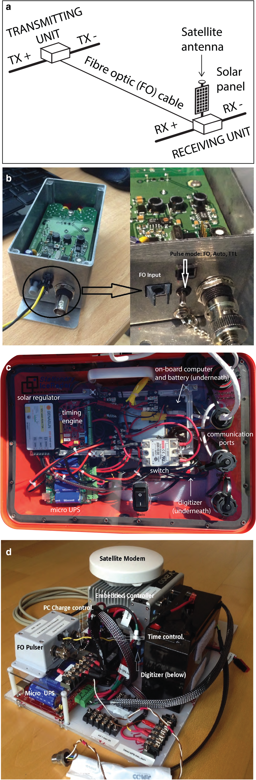
Fig. 1. Typical sIPR configuration and components. (a) Diagram of typical field deployment. (b) Redesigned transmitter with auto, TTL and FO pulse modes. (c) Receiver deployed on Kaskawulsh Glacier in 2017 mounted in a protective case (lid open view) with components visible through the polycarbonate operator panel. (d) Receiver (during construction) deployed on Petermann Ice Island in 2015.
Transmitting unit
We use an impulse transmitter (Fig. 1b) that produces a ±600 V pulse with a 2 ns rise time. The transmitter design (Bennest Enterprises Ltd.) is based on that of Narod and Clarke (Reference Narod and Clarke1994), but has an adjustable pulse repetition frequency (PRF, e.g. 64, 128, 256 and 512 Hz). It can operate in one of three modes: (1) auto, where pulses are produced continuously at a prescribed PRF, (2) TTL (transistor–transistor logic), where an external square wave of amplitude 3.3–5.0 V triggers the transmitter at a rate prescribed by the square wave frequency and (3) fibre optic (FO), where an optical pulse of a given frequency is used to trigger the transmitter. The sIPR deployments described here use the FO, permitting the transmitter to sleep in the absence of an optical pulse. In sleep mode, transmitter current consumption is about 1.7 mA (at 12 V DC), compared to ~150 mA (at 12 V DC) while pulsing (for 512 Hz PRF). The duration of a radar acquisition is a few seconds, so the transmitting unit largely remains in sleep mode. The optical pulser draws a current of 0.3 mA when operating and none while asleep.
Receiving unit
The sIPR receiver (Figs 1c and d) comprises a 12-bit digitizing electronics board (Pico 4227) and a computing board (Moxa) that controls the radar acquisitions, an optical pulse generator to drive the transmitter via the FO link (set to 128 Hz PRF) and a micro-UPS (uninterruptible power supply). The ice-island deployment (Fig. 1d) also included an on-board GPS unit (Garmin 18x OEM) and a low-power satellite communication module (Iridium 9602). The system's duty cycle is managed by a timing module and a solid-state switch that controls the on–off system states. We tested several variations of the timing module, from simple digital timing circuitry to micro-controller-based timing (Atmega328P) paired with a real-time clock (RTC). We found the latter to be the most flexible, with time settings adjustable via firmware, and to require the least power (<1 mA during sleep). The micro-UPS (Linear Computing Inc.) was introduced to minimize the risk of a power brown-out, which would lead to uncontrolled system shutdown. In case of failure of the power supply, the micro-UPS can sustain the radar operation for around one minute, leaving enough time to complete operations underway and execute an orderly shutdown. GPS and satellite communication boards are also interfaced with the main on-board computer. All components are operated by purpose-built software.
Once the system is deployed, the timing module wakes up at regular intervals (e.g. minutes or hours, depending on the settings) and checks if it is time to power up the radar for a measurement (e.g. every few hours) based on the RTC time. When a measurement is indicated, the timing module turns on a solid-state switching circuit that delivers power to the micro-UPS, which in turn powers-up all the other components. The FO pulser begins pulsing through the FO link and drives the transmitter. With all of the above components running, the system is ready to acquire and waits for an incoming trigger that can either be the direct wave, or a FO-synchronized TTL pulse (depending on system set-up). Once the required number of stacks is obtained, the data are locally saved and may be transferred via the satellite link. Prior to stacking, the noise floor of the system is ~−67 dBm, with thermal noise being the largest contributor.
Software
The sIPR software was developed based on the platform designed to control a similar radar system used for common-offset surveys (Mingo and Flowers, Reference Mingo and Flowers2010). Software modules were added to address the functionality of the new components and enable autonomous operation of the system. For example, the micro-UPS is interfaced via its serial port to the main computer so that power usage and state information is retrieved continuously while the radar tasks are running. See Appendix A for a description of the software control of satellite communications.
Special consideration was given to triggering for unattended long-term deployments during which changing environmental conditions (e.g. melting snow/ice surfaces) or changes in system power (e.g. due to limited recharging capability of the transmitter) may alter the amplitude of the direct wave. The software includes an adaptive trigger-level scheme in which multiple trigger levels can be prescribed. During each acquisition, the system steps through these trigger levels in decreasing order until it successfully acquires a predefined fraction of the requested number of triggers for a given stack, typically 256, 512 or 1024. The direct-wave amplitudes are generally consistent on timescales of days, but surface coupling of any system can change over deployment periods of weeks to months, particularly from the onset of melting to the completion of snow melt. Such changes must be considered if performing amplitude analysis. The adaptive triggering scheme merely increases the probability that the expected waveform is captured even in the presence of a declining direct-wave amplitude as measured by the receiver. See Appendix B for a description of software provision for dual-channel capture of the full amplitude of the direct wave.
Field Deployments and Results
Different implementations of the sIPR system described above were deployed in two remote locations in sub-Arctic and Arctic environments in northern Canada from 2014–2017. Below we describe the study-area locations and instrument configurations, along with deployment results and preliminary data analysis to illustrate applications of the sIPR. Our focus here is a proof of concept of the instrument, rather than a comprehensive description of the scientific problems being addressed.
Kaskawulsh Glacier, Yukon, Canada
Study area description
The Kaskawulsh Glacier is a major outlet draining the icefields of the St. Elias Mountains (Fig. 2), which straddle the Canada–US border and have >25,000 km2 of ice cover (Kienholz and others, Reference Kienholz2015). The glacier is ~70 km long, from its divide with the Hubbard Glacier to its terminus at ~830 m asl, with an estimated catchment area of 1095 km2 (Foy and others, Reference Foy, Copland, Zdanowicz, Demuth and Hopkinson2011). Its thermal regime has not been explicitly studied, but has been described as both polythermal and temperate in the accumulation area (see Holdsworth, Reference Holdsworth1965). The glacier is also one of few large outlets in the region that is not known to surge (Clarke and others, Reference Clarke, Schmok, Ommanney and Collins1986). Approximately 35 km upglacier from its terminus, on the north side just below the confluence of the north and central tributary arms, the Kaskawulsh Glacier dams an ice-marginal lake (60°46′ N, 139°07′ W) that is observed to fill and drain annually (e.g. Kasper, Reference Kasper1989; Kasper and Johnson, Reference Kasper and Johnson1991; Bigelow and others, Reference Bigelowin press). In the vicinity of the lake, ice-surface elevations are 1600–1650 m asl, and measured ice thicknesses exceed ~650 m 1 km from the ice front (Bigelow and others, Reference Bigelowin press). Time-lapse photographs (unpublished data, C. Schoof and C. Rada) reveal pronounced changes in lake-proximal ice-surface elevation associated with lake filling and drainage, indicative of a floating ice shelf and a subglacial component to the lake. We identified the study area as a location that might furnish temporally varying englacial/subglacial properties observable with the sIPR.
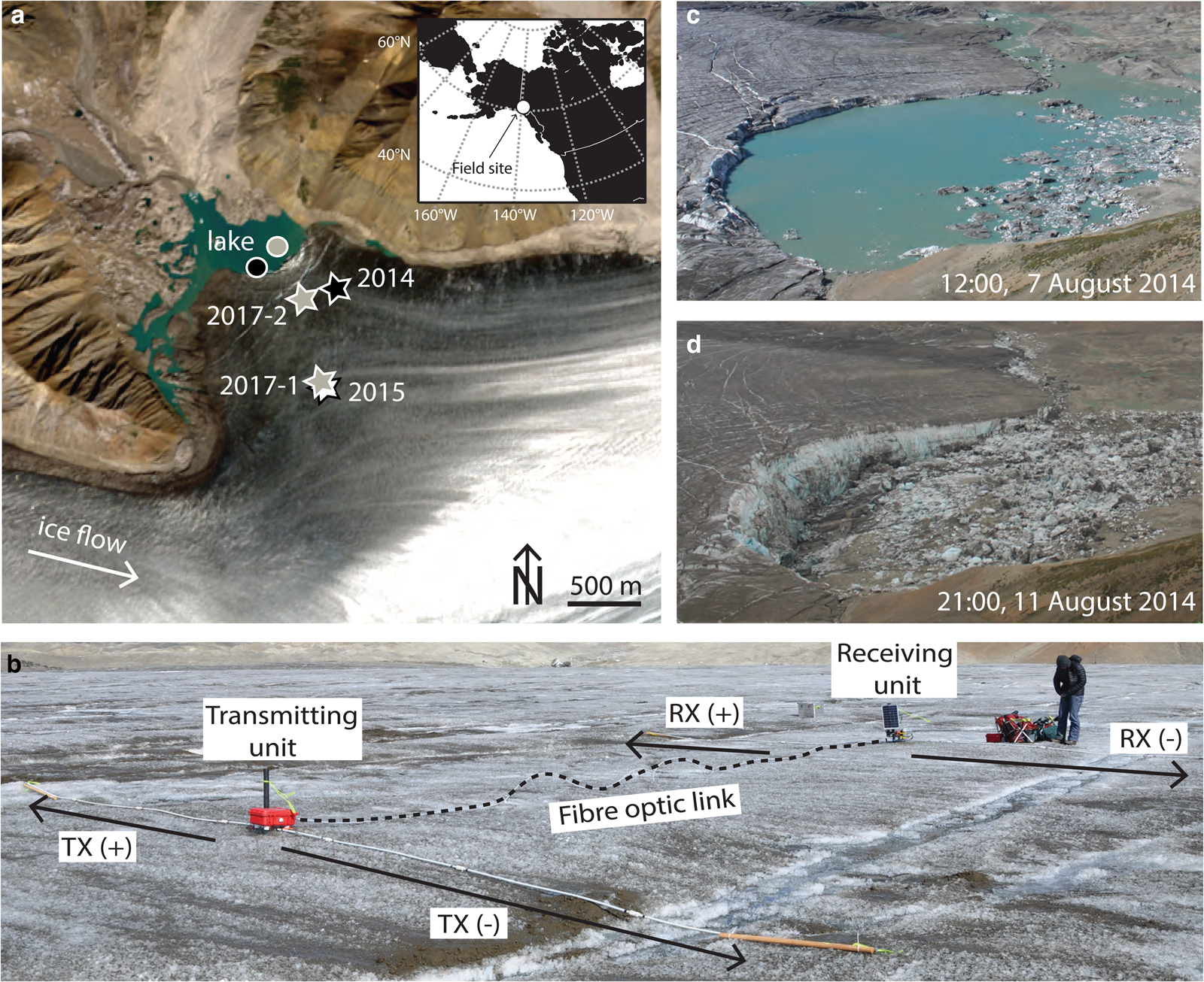
Fig. 2. Deployment locations and configuration of sIPR near an ice-dammed lake on the Kaskawulsh Glacier, St. Elias Mountains. (a) Kaskawulsh Glacier and adjacent ice-dammed lake with sIPR deployment locations for 2014 (black star), 2015 (white star) and 2017 (grey stars). 2015 and 2017-1 sIPRs are co-located where the ice thickness is ~380–390 m. Ice thickness is ~210–220 m in the vicinity of 2017-2 and 2014. Approximate locations of pressure sensors are shown as circles for 2014 (black) and 2017 (grey). Imagery from Sentinel-2 (8 August 2017, Copernicus Sentinel data 2017, processed by ESA). The inset shows study area in southwest Yukon, Canada. (b) Annotated photograph of 2015 sIPR deployment with transmitting (TX) and receiving (RX) antennas (credit: A. Pulwicki). View toward lake. (c) Lake near maximum stage, 12:00 on 7 August 2014. (d) Lake empty, 21:00 on 11 August 2014. Time-lapse photographs in (c) and (d) courtesy of C. Schoof and C. Rada.
Instrument deployment
Four sIPR devices were deployed on the Kaskawulsh Glacier, within 1 km of the ice-dammed lake, in three separate campaigns: 26 July–7 Sept 2014, 15 July–27 August 2015 and 15 June–11 September 2017 (Fig. 2). sIPR deployments in 2014 and 2015 were intended as proof-of-concept, while the 2017 deployments were part of a larger project to study the lake filling and drainage cycle involving other geophysical and hydrometeorological instrumentation (Bigelow, Reference Bigelow2019; Bigelow and others, Reference Bigelowin press). The 2014 and 2017 deployment periods spanned the annual lake drainage event, while the 2015 deployment occurred after lake drainage.
In all years, transmitting and receiving units were housed in waterproof cases, separated by 12–15 m and tethered to poles drilled several metres into the ice (Fig. 2b). The tether design permitted the cases to remain in contact with the melting ice surface. Antennas of 10 MHz centre frequency were housed in polyethylene tubing or garden hose, oriented parallel to one another, and weighted or tethered at the ends to minimize motion. The systems were oriented with antennas roughly perpendicular to both the dominant direction of crevasses and the lake–ice interface. In 2014 and 2015, the transmitting unit was powered by a 12 V, 6.6 Ah battery, while the receiving unit was powered by a 12 V, 7 Ah battery and a 10 W solar panel. In 2017, 7 and 10 Ah batteries were used for transmitting and receiving units, respectively, each with 10 W solar panels. The timing module wake-up interval was set to 4 h in 2014 and 3 h in 2015 and 2017. In order to minimize potential cross-talk between the two 2017 systems, the system timers were offset by 15 min. No satellite communication was used at this site.
In 2014 a pressure transducer (U20-001-03 Onset Hobo Water Level Logger, 0–76 m range) was deployed on a dyneema cable in the lake adjacent to the ice cliff, and tethered to a pole drilled into the ice. In 2017, water pressure was measured with a Geokon 4500-HD 7.5 Megapascal (MPa) sensor deployed at the lake bed and connected to a data logger on shore. Water-pressure measurements were converted to relative lake level, after correction for atmospheric pressure, using a water density of 1000 kg m−3. The 2014 data represent water level relative to the ice surface, while the 2017 data represent water level relative to a datum that is presumed fixed.
Results and preliminary analysis
The sIPR system operated autonomously for 36 and 44 days in 2014 and 2015, respectively. In 2017, the systems operated autonomously for 68 and 77 days. Over 4 m of surface melt, combined with tethering poles that were too flexible, led to the rotation of the solar panels toward the ice surface in 2017 (Bigelow, Reference Bigelow2019). Consequently, the systems lost power ~1 month after the solar panels became obscured. Here we focus on the 2014 and 2017 results, as marked temporal changes in the radargrams before, during and after lake drainage are visually apparent (Fig. 3). Furthermore, the 2017 deployment was complemented by numerous other instruments, including shallow borehole water-pressure sensors, GPS stations and time-lapse cameras, all of which provide data to corroborate our interpretations (Bigelow and others, Reference Bigelowin press).
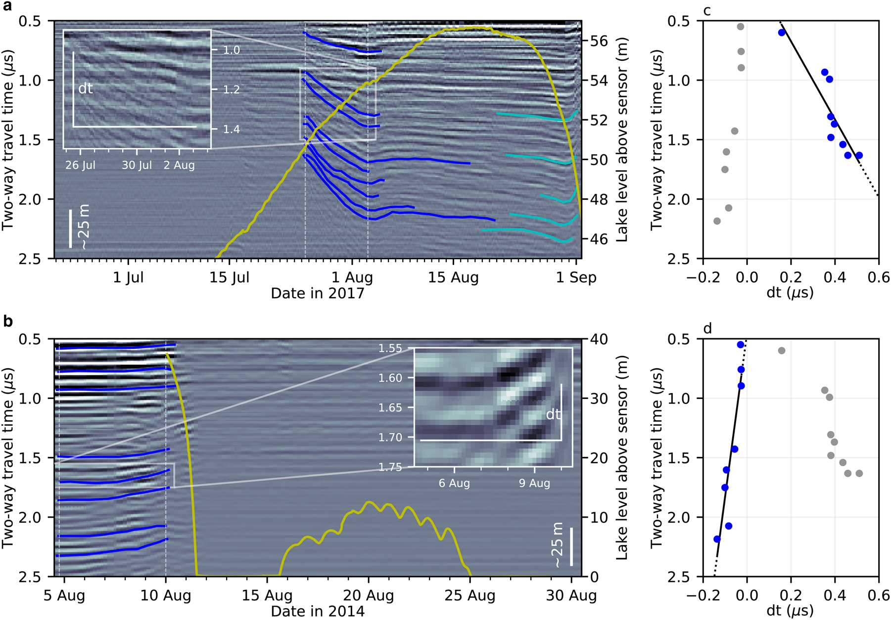
Fig. 3. Selected results of sIPR deployments on the Kaskawulsh Glacier during various stages of lake filling and drainage. (a) Seventy-four of the 77 days of record from sIPR 2017-2 (nearest the ice front; Fig. 2). Record spans lake filling and the onset of lake drainage. The lake level above the pressure sensor shown in yellow (right axis). Radar data have been dewowed and smoothed using a 7 × 7-point moving-average filter. Both flat and dipping reflectors can be identified in the data. Dipping reflectors are digitized during the period of rapid filling (blue) and during lake drainage (cyan). Vertical white dashed lines indicate the period over which dt in (c) is calculated. The scale bar shows approximate ice depth assuming a radar velocity of 1.68 × 10⁸ m s−1. Inset: enlarged view of dipping reflectors with dt defined. (b) As in (a) but for 26 of the 36 days of record in 2014. Record spans the lake drainage. Several prominent rising reflectors are digitized (blue). Lake-level record (yellow line, right axis) begins after the onset of lake drainage. The flat line corresponds to atmospheric pressure, thus lake level below sensor position. (c) Linear regression of dt (blue dots) on mean travel time for 2017 data. dt is the change in the two-way travel time for digitized reflectors (blue) in (a) between 25 July and 3 August 2017 (vertical white dashed lines). The dashed line in (c) is extrapolation of regression (solid line). Grey dots represent 2014 data. (d) As in (c) but for reflectors in (b) between 4 and 10 August 2014. Grey dots represent 2017 data.
Lake filling and the onset of drainage were captured in 2017 (Fig. 3a), while only drainage was captured in 2014 (Fig. 3b). Lake-full and lake-empty conditions correspond to high and low radar internal reflection power, respectively, while periods of active filling or drainage are associated with downward or upward deflections of clearly identifiable reflectors. Much of the 2017 record prior to mid-July is characterized by low reflection power (Fig. 3a). Abrupt changes in reflection power at various depths occurred on 16 and 26 July 2017, which, based on borehole water-pressure data, measured ice-surface displacements and time-lapse imagery, we interpret as changes in englacial storage associated with fracturing events (Bigelow and others, Reference Bigelowin press). Significant downward deflection of reflectors commenced on 27 July 2017. A temporary reversal of this downward deflection occurred on 3 August 2017, commensurate with a brief drop in lake level (inflection in the lake-level curve, yellow line, Fig. 3a). Downward deflection then continued, but at a lower rate than prior to 3 August 2017, until another sharp reversal occurred on 30 August 2017 during rapid lake drainage. The dipping reflectors overprint flat reflectors that appeared unaffected by lake filling and drainage. Given the broad lobes of the antenna radiation pattern, it is not surprising that the sIPR samples an ice volume that does not respond uniformly to these perturbations.
In 2014, internal radar reflection power dropped sharply between 9 and 11 August (Fig. 3b) while the lake was draining, and stabilized at lower values once the lake was empty. Upward dipping reflectors are clearly visible prior to 10 August. The onset of the 2014 lake drainage was estimated from time-lapse images to have commenced by mid-day on 7 August (Fig. 2d). After lake drainage, the lake-level record shows a period of partial refilling characterized by diurnal variations (yellow line, Fig. 3b). There is no obvious response in the radiostratigraphy, presumably due to the lack of hydraulic communication between the lake at these levels and the englacial volume sampled by the sIPR.
The strong association between temporally varying radiostratigraphy and pronounced lake-level changes in both 2014 and 2017 argues for a common explanation. We hypothesize that changes in englacial storage, associated with lake filling and drainage, produce changes in the depth-averaged radar velocity (e.g. Macheret and others, Reference Macheret, Moskalevsky and Vasilenko1993) that are expressed as upward or downward deflections of reflectors fixed in space (Figs 3a and b). Near-surface reflectors exhibit almost no deflection (Figs 3a and b) compared to reflectors at depth, consistent with the hypothesized change in depth-averaged radar velocity. Evaluated over a common time interval (between vertical dashed white lines in Figs 3a and b), the magnitude of the deflection (dt) of individual reflectors is linearly related to the travel time, as expected (Figs 3c and d).
If we assume the reflectors are indeed spatially fixed and their deflection is caused by a change in depth-averaged radar velocity associated with a change in englacial water content, we can estimate the change in porosity ϕ of the ice column as (Looyenga, Reference Looyenga1965):
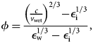
with c = 3.0 × 10⁸ m s−1 the speed of light, v wet the radar velocity of wet ice, εi = 3.2 the dielectric constant of ice and εw = 81 the dielectric constant of water. Here we assume that water is injected into the ice by hydrofracture and that the resulting fracture network closes when drained, such that we can omit any treatment of air-filled voids. A more comprehensive treatment would allow some persistence of air-filled voids at shallower depths. Under these assumptions, we calculate v wet as
where v 0 is the velocity at two-way travel time t 0, and dt is estimated as illustrated in Figures 3a and b. For an individual reflector in the 2017 dataset, t 0 is the two-way travel time corresponding to the initial position (depth) of the reflector prior to deflection, where we assume a depth-averaged radar velocity v 0 = 1.68 × 10⁸ m s−1. In the 2014 dataset, t 0 is the two-way travel time corresponding to the final position (depth) of the reflector after deflection, where we make the same velocity assumption as above. The calculation in Eqn (2) is approximate, intended as an illustration of the analysis that could be pursued with these datasets.
Using the digitized reflectors in Figure 3b, Eqn (1) yields a decrease in porosity (i.e. water content) of 1.6 ± 0.4% (mean ± standard deviation) from 18:00 on 4 August to 00:00 on 10 August 2014 associated with the lake drainage. Similarly, the digitized reflectors in 2017 (Fig. 3a) yield an increase in water content of 9.9 ± 1.3% (mean ± standard deviation) from 12:00 on 25 July to 04:00 on 3 August 2017. These standard deviations represent only the variability of the result between individual traced reflectors; they do not include systematic uncertainties associated with the method.
We speculate that ϕ continues to increase until the deflection changes sign during lake drainage (cyan lines, Fig. 3a), but it is difficult to unambiguously trace individual reflectors across the whole month of August. A few percent water content is typical of values reported in the literature (e.g. Moore and others, Reference Moore1999; Bradford and others, Reference Bradford, Nichols, Mikesell and Harper2009; Endres and others, Reference Endres, Murray, Booth and West2009), while values approaching 10% are not unprecedented (e.g. Macheret and Glazovsky, Reference Macheret and Glazovsky2000; Hart and others, Reference Hart, Rose and Martinez2011) and are supported by independent estimates made from water-balance calculations of the lake catchment (Bigelow, Reference Bigelow2019). Bigelow and others (Reference Bigelowin press) pursue a much more extensive analysis of the role of englacial storage in the 2017 lake filling and drainage cycle using additional data from shallow borehole pressure sensors, GPS stations, time-lapse imagery and repeat common-offset radar surveys.
Petermann Ice Island-A-1-f, Nunavut, Canada
Study area description
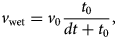
Petermann Ice Island (PII)-A-1-f was a fragment of the ~136 km2 tabular iceberg that calved from the Petermann Glacier in northwest Greenland (80°45′ N, 60°45′ W, Fig. 4a) in July 2012 (Crawford and others, Reference Crawford, Mueller, Desjardins and Myers2018) with a reported average thickness of 182 ± 16 m (Münchow and others, Reference Münchow, Padman and Fricker2014). PII-A-1-f was first observed on 10 September 2013 after PII-A-1, the largest fragment persisting after the Petermann Glacier calving event, fractured in Nares Strait (personal communication, L. Desjardins). The ice island followed the common route of previous ice islands sourced from northwest Greenland's floating ice tongues, drifting south through Nares Strait and then being directed through the western sector of Baffin Bay by the southerly Baffin Current (Newell, Reference Newell1993; Crawford and others, Reference Crawford2016, Reference Crawford, Mueller, Desjardins and Myers2018). The 14 km2 PII-A-1-f became grounded in October 2014 off the east coast of Baffin Island at ~67°23′ N, 63°18′ W, where it was first accessed in October 2015 (Fig. 4a and b) (personal communication, S. Tremblay-Therrien). The ice island deteriorated to ~9 km2 over the duration of the sIPR data collection period, while pivoting and slowly translating along the underwater ridge on which it was lodged (Crawford, Reference Crawford2018).
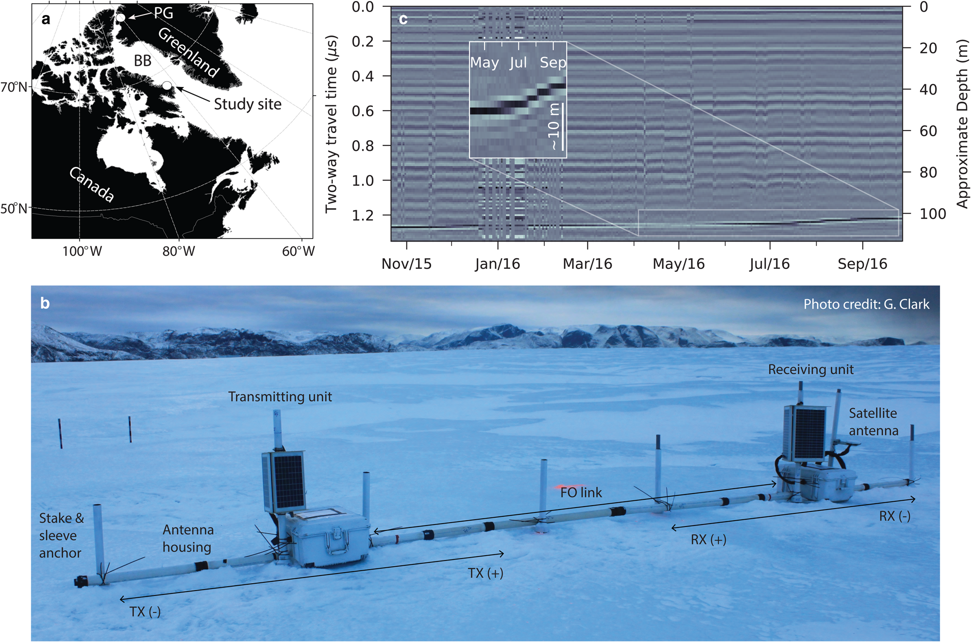
Fig. 4. Deployment location, configuration and results of sIPR on Petermann Ice Island (PII)-A-1-f. (a) Location of the grounded ice island in Baffin Bay (BB) and its Peterman Glacier (PG) origin. (b) Annotated photograph of PII-A-1-f sIPR deployment in 2015. (c) sIPR data collected from November 2015–September 2016. Some received data from Jan–Feb 2016 were corrupted. A change in the ringing pattern in May is attributed to attempts to change system grounding during a site visit.
Instrument deployment
The PII-A-1-f sIPR deployment site was reached on 20 October 2015 by helicopter from the Canadian Coast Guard Ship (CCGS) Amundsen icebreaker during Leg 4 of ArcticNet's annual scientific research cruise. The sIPR was installed on a ridge toward the centre of the ice island and was anchored to a series of vertical PVC sleeves that slide over ~ 3 m × 2.5 cm PVC stakes drilled into the ice (Fig. 4b). As in the Kaskawulsh Glacier deployments, this design allowed the system to remain in contact with the melting ice surface. A Campbell Scientific digital camera (CC5MPX) and a Garmin GPS (16X-HVS) were deployed on a nearby weather station to monitor the position of the sIPR and the movement of the ice island over time (Crawford, Reference Crawford2018).
The waterproof cases containing the transmitting and receiving units were installed in-line with ~4.8 m separation and connected by a 5 cm diameter PVC tube that housed the 40 MHz antennas (Fig. 4b). A centre frequency of 40 MHz was chosen by considering the intended penetration depth, the desired depth resolution, the anticipated surface conditions in both winter and summer (including the potential for surface water), the receiver sampling rate (125 MS s−1), the amount of data produced at this rate and the data transmission via satellite. One 12 V, 55 Ah battery and three 10 W solar panels powered the transmitter, while two 12 V, 35 Ah batteries and three 20 W solar panels powered the receiver. These battery capacities were chosen based on the system's power budget and the ~4 month duration of low light conditions in the region. Each set of solar panels was arranged with a triangular base to ensure power generation regardless of the orientation of the ice island relative to incoming solar radiation (Fig. 4b). The system's timer switch initiated daily data acquisition and remote transmission via a RockBLOCK+ satellite modem over the Iridium satellite network. Daily data collection continued until September 2016.
Results and preliminary analysis
The 344-day data set obtained on PII-A-1-f spans all seasons including the polar winter (Fig. 4c). Daily radar acquisition and data transmission were uninterrupted with few exceptions, the longest being a period in January–February 2016 during which some corrupted data were received. Satellite communication failure due to power shortages is suspected in the transmission interruptions. Regular data transmission was reestablished after this period when battery power capacity was restored through the solar panels. Radar data during this transmission outage were recorded to the sIPR on-board storage.
The sIPR radargram exhibits a prominent and persistent reflector that indicates ice thickness was initially ~106 m. Our interpretation of the ice–ocean interface was corroborated by roving surveys with a mobile IPR system and multi-beam sonar scans acquired by the CCGS Amundsen. Changes in ice-column thickness are visually detectable beginning in November 2015 as this reflector is deflected slightly upward. Few changes in radiostratigraphy are evident in the sIPR record from PII-A-1-f, but ice-island thinning of 4.7 m over 11 months was documented and has been analysed in detail by Crawford (Reference Crawford2018). While the digitizer sampling rate limits the vertical resolution of ice-depth soundings with the sIPR, further analysis can be used to extract information from the bed return.
The sampling rate was constrained by the need to transmit data by the satellite link (Appendix A) and the simultaneous dual-channel input scheme (see Appendix B). A sampling rate of 125 MS s−1 corresponds to a Nyquist frequency of 62.5 MHz, which while above the 40 MHz centre frequency of the ice-island system, is not sufficient to adequately render the higher frequency content of the signal (~10–20 MHz sideband above the peak) (Fig. 4c). A sampling frequency of at least four times the high frequency content is preferred in practice. Assuming a radar velocity of 1.68 × 10⁸ m s−1, the 8 ns sampling interval (two-way travel time for a sampling rate of 125 MS s−1) corresponds to an ice thickness of 0.67 m.
We suggest that the effective resolution of measured ice-thickness changes can be reduced below 0.67 m by exploiting amplitude variations in the bed return as measured by the system's ADC. To illustrate how this might work, we compute the signal power around the bed (effectively an uncorrected bed reflection power) for synthetic radargrams in which ice thickness is changing at a constant (Fig. 5a) or variable (Fig. 5b) rate. In both cases, the bed reflector is synthesised using a Ricker wavelet centred at 40 MHz and sampled at 125 MS s−1. The variable rate of the ice-thickness change imprints itself on the reflection-power time series as horizontal stretching and compression compared to the constant rate case. When applied to the real data (Fig. 5c), this analysis yields results that bear some qualitative resemblance to the variable-rate case above, suggesting that information about the rate of the ice-thickness change is indeed encoded in the quasi-periodic variations of bed reflection power. A transfer function would be required to estimate the actual rates. Similar periodic amplitude variations are not found in the direct wave nor in calculated internal reflection power, implying that these variations are dominated by the transition from one ADC level to the next.
Fig. 5. Bed reflection power (BRP) characteristics during sIPR-detected changes in ice-island thickness. (a) Synthetic data with a constant rate of the ice-thickness change. The inset shows Ricker wavelet sampled at 125 MS s−1. (b) As in (a) but for the variable rate of the ice-thickness change. (c) Real data from PII-A-1-f ice island. The inset shows sample wavelet. The solid white line on radargram indicates a plausible series of bed picks. The solid line in lower panel shows smoothed BRP (dots).
Summary and Outlook
We have described the design and deployment of an impulse-type stationary ice-penetrating radar (sIPR) system suitable for use in a variety of environments, from temperate glaciers to cold ice shelves. Particular consideration was given to low-power operation suitable for high-latitude winter conditions, reliable autonomous performance for deployment periods approaching a year and the ability to transmit data via satellite. The Arctic ice-island deployment represents the longest test of the sIPR system to date. Its success demonstrates the system's suitability for cold polar environments, in addition to more temperate environments characterized by high melt rates.
The Kaskawulsh Glacier sIPR deployments from 2014–2017 revealed time-variable radiostratigraphy in the vicinity of an ice-dammed lake that we hypothesize arises from changes in englacial water storage. Time-variable changes in internal reflection power have been used in combination with other datasets to understand the 2017 lake filling and drainage cycle (Bigelow, Reference Bigelow2019; Bigelow and others, Reference Bigelowin press). Devising mounting structures that can cope with 4–5 m of melt while the sIPR systems were unattended proved to be the greatest challenge in this environment. The PII-A-1-f sIPR deployment holds promise for future data collection from drifting ice islands that are not readily and regularly accessible. Multiple ice islands have since calved from floating ice shelves in the Arctic and Antarctic, including from Petermann Glacier where another large calving event is expected. The generation of these tabular icebergs presents new opportunities to monitor their deterioration with in-situ instrumentation such as the sIPR system described here.
Two-way telemetry would be a useful addition to future systems to allow remote adjustment of control settings, and some debugging capability in the case of unexpected system behaviour. Installation of an array of receivers or transmitters (e.g. Young and others, Reference Young2018), rather than just a single pair, would provide a richer dataset that may be particularly useful for studies like that of the ice-dammed lake, where spatial anisotropy and heterogeneity of the time-variable signal may be expected.
Acknowledgments
L. Mingo acknowledges the SR&ED Tax Incentive Program of the CRA for offsetting some R&D costs of the sIPR. G. Flowers and D. Bigelow are grateful to NSERC, CFI, CSA, NSTP, PCSP and SFU for funding, Kluane First Nation, Yukon Government and Parks Canada for access to Yukon field sites and S. Williams, L. Goodwin, A. Pulwicki, J. Crompton, F. Beaud and Canadian astronaut D. Saint-Jacques for support and field assistance. C. Schoof and C. Rada provided time-lapse imagery and 2017 water-pressure data. A. Crawford and D. Mueller acknowledge funding from NSERC, Transport Canada, PKC/NSTP and the Garfield Weston Foundation, as well as support from ArcticNet, the CCGS Amundsen crew and pilots O. Talbot, A. Roy and G Carpentier. The following people are thanked for their laboratory and field assistance: G. Clark, J. Moesesie, J. Gagnon, T. Desmeules, L. Copland, A. Dalton, J. Rajewicz, H. Jacques, L. Candlish, N. Therieault, A. Cook, A. Burt, C. Bernard-Grand'Maison, L. Braithwaite, A. Garbo, I. Burnett and Canadian astronaut and Governor-General J. Payette. Thanks to two anonymous reviewers for their helpful feedback.
Appendix A. Software Control of Satellite Communications
Data transmission by the satellite link was used in the ice-island deployment, under the assumption that the system might be unrecoverable. The satellite communication task requires several steps to successfully and efficiently transmit the radar data. The Iridium modem used in the Petermann Ice Island deployment operates with the Short Burst Data (SBD) service, which can only transmit up to 340 bytes per message, in part due to its low power requirements. It was also important to minimize the volume of transmitted data in order to reduce transmission time and cost. The data comprising a single radargram usually exceed this payload, depending on the sampling rate, record length (set based on expected ice thickness) and accompanying meta-data. Data compression is therefore used to reduce the size of the raw data. For example, with a sampling rate of 125 MS s−1 and a listening time of 1.6 μs (sufficient to sound ice ~130 m thick), the uncompressed data are coded over ~2100 bytes, which are compressed to ~600 bytes; the actual compression performance also depends on the data. The compressed data are then split into subsets that are transmitted separately. In this example, the uncompressed data would require seven SBD messages, compared to two messages for the compressed data. This step requires the addition of protocol fields (e.g. unique identification and numbering) to each data subset in order to enable the reconstruction of the full dataset. Protocol fields increase the message overhead but are necessary, because there is no guarantee that messages will be received in the order sent. A message queue is also implemented in the software to save messages locally and allow for future transmission attempts, should the data acquisition or satellite communication tasks be interrupted (e.g. due to the radar system reaching its maximum allowable wake time or the lack of satellites in view at transmit time).
Appendix B. Dual-channel acquisition for direct-wave amplitude preservation
For some analyses of englacial/subglacial properties from sIPR data, it is desirable to capture the full amplitude of the direct wave without compromising the detection and characterization of low-amplitude reflectors. The software therefore includes an alternative acquisition mode in which two channels that differ only in their preset input ranges are used as dual inputs. Typically, the first channel would be set to a greater range intended to capture the full amplitude of the direct wave, while the second channel would have the lowest available input range intended to improve the resolution of low-amplitude reflectors; the direct wave would therefore appear clipped in the second channel. A typical setting for the lowest range would be ±50 mV distributed over 12 bits, leading to 212 = 4096 discrete levels. With 256 stacks, the calculated improvement in resolution due to stacking is 4 bits (22n = 256), leading to a total of 12+4=16 bits of effective resolution, or 65,536 discrete levels.
With the specific acquisition hardware we used, simultaneously sampling on two input channels reduces the maximum sampling rate from 250 to 125 MS s−1. An alternative approach implemented with the latest deployment (in the field at the time of writing) is to perform two consecutive acquisition sessions instead of one, just a few seconds apart. One session is set with a large input range to capture the full amplitude of the direct wave (i.e. 100–200 mV), while the other is set with a small input range (i.e. 50 mV) for best resolution. This approach takes advantage of the maximum allowable sampling rate, in this case 250 MS s−1, and assumes that no change occurs over the brief interval between sessions.


 Open access