
Abstract
We report a quantum Monte Carlo study of the phase transition between antiferromagnetic and valence-bond solid ground states in the square-lattice S = 1/2 J–Q model. The critical correlation function of the Q terms gives a scaling dimension corresponding to the value ν = 0.455 ± 0.002 of the correlation-length exponent. This value agrees with previous (less precise) results from conventional methods, e.g., finite-size scaling of the near-critical order parameters. We also study the Q-derivatives of the Binder cumulants of the order parameters for L2 lattices with L up to 448. The slope grows as L1/ν with a value of ν consistent with the scaling dimension of the Q term. There are no indications of runaway flow to a first-order phase transition. The mutually consistent estimates of ν provide compelling support for a continuous deconfined quantum-critical point.
Export citation and abstract BibTeX RIS
Among the many proposed exotic quantum states and quantum phase transitions beyond the Landau–Ginzburg–Wilson (LGW) paradigm in two dimensions,[1–3] the deconfined quantum critical point (DQCP)[4] is special because it has concrete lattice realizations in sign-free "designer models" accessible to quantum Monte Carlo (QMC) simulations.[5] Indeed, the first hints of an LGW-forbidden continuous transition between antiferromagnetic (AFM) and spontaneously dimerized valence-bond solid (VBS) ground states came from QMC simulations,[6] and following the DQCP concept (which builds on previous works on VBS phases and topological defects[7–13]) numerous additional studies have been reported. The most compelling results for DQCP physics have been obtained with J–Q models,[14–27] which are Heisenberg antiferromagnets in which the exchange of strength J is supplemented by multi-spin couplings of strength Q that induce singlet correlations and eventually cause spontaneous dimerization. The space-time loop structure employed in QMC simulations[28–30] can also be used to formulate analogous classical three-dimensional loop models, which exhibit behaviors very similar to the J–Q models.[31,32]
Even though very large lattices have been studied, with linear size L up to 256 for the J–Q model[18,26] and twice as large for the loop model,[32] it has not yet been possible to draw definite conclusions on the nature of the AFM–VBS transition. While no explicit signs of a first-order transition have been detected in the best DQCP candidate models (in contrast to intriguing discontinuous transitions with emergent symmetry in related models[33–35]), some observables exhibit scaling behaviors incompatible with conventional quantum criticality. Such behaviors have been interpreted as runaway flows toward what would eventually become a first-order transition on lattices even larger than those studied so far.[16,22,36] Another proposal is that the DQCP is even more exotic than initially anticipated, with novel relationships between critical exponents originating from the presence of two divergent length scales[26]—in addition to the standard correlation length ξ, there is a larger scale ξ' associated with a "dangerously irrelevant" perturbation and emergent U(1) symmetry of the near-critical VBS fluctuations in the DQCP scenario.[4,37] The weak first-order scenario has attracted attention in the context of non-unitary conformal field theories (CFTs), which have critical points in the complex plane.[38–41] In this scenario, the AFM–VBS transition is a "walking" first-order transition,[42,43] where the renormalization-group flow (which is also manifested in finite-size scaling) is affected by the inaccessible nearby critical point and only slowly "walks" to a first-order instability.
In support of the weak first-order scenario, the J–Q and loop models are often invoked as supporting evidence, though there are no concrete predictions that have been compared with the numerical results. In the absence of any quantitative tests or clear signs of discontinuities or coexistence state in the lattice models, the walking scenario should not be accepted as the final word on the fate of the DQCP. Here we will show that the cited[39–41] large scaling corrections affecting estimates of the correlation length exponent ν[21,26,32] are not precursors to a first-order transition. We reach this conclusion by extracting ν from the scaling dimension of the relevant field of the model. The corresponding correlation function exhibits only small scaling corrections and delivers an exponent compatible with results based on Binder cumulants; ν = 0.455(2). Given the well behaved estimators of ν, a continuous transition is the most likely scenario.
To set the stage, we briefly summarize some standard facts on critical scaling. Consider a Hamiltonian Hc tuned to a quantum critical point to which a perturbation is added that maintains all the symmetries of Hc;
where r denotes the lattice coordinates and D(r) are local operators. Normally H is written in a form with some tunable parameter g such that, for some critical value g = gc, H(gc) = Hc and δ = g – gc. We assume that the system develops long-range order when δ > 0, with an order parameter m(r) such that 〈m〉 = 〈m(r)〉 ∝ δβ for small δ > 0 and m = 0 for δ < 0. The critical exponent β depends on the universality class of Hc in the thermodynamic limit. On either side of the phase transition, the exponential decay of the correlation function Cm(r) = 〈m(0)m(r)〉 – 〈m〉2 defines the divergent correlation length, ξ ∝ |δ|−ν. At δ = 0, the correlation function takes the critical form Cm(r) ∝ r−2Δm, where Δm = β/ν is the scaling dimension of the operator m.
In QMC calculations ν is typically extracted using finite-size scaling of some dimensionless quantity, such as the Binder ratio R = 〈M4〉/〈M2〉2, where M = ∑r m(r). Neglecting scaling corrections, in the neighborhood of the critical point we have R(δ,L) = R(δL1/ν), by which ν (and the critical point gc if it is not known) can be obtained from data for different values of δ and L. A less common method is to use the relation 1/ν = d – ΔD, where d is the space-time dimensionality (here d = 3) and ΔD is the scaling dimension of the perturbing operator D in Eq. (1). The scaling dimension can be obtained from the power-law decay CD(r) ∝ r−2ΔD of the correlation function CD(r) = 〈D(0)D(r)〉 – 〈D〉2 at gc.
It is not clear to us why ν is not commonly extracted from CD(r), but there are two potential drawbacks: (i) Often ΔD is rather large, e.g., in the case of the O(3) universality class (of which we will show an example below) ΔD ≈ 1.6, so that the correlation function decays rapidly and is difficult to compute precisely (with small relative statistical errors) at large r. (ii) The operator D is often off-diagonal and may appear to be technically difficult to compute. However, although the latter issue is absent in simulations of classical systems, the scaling dimension ΔD is still normally not computed.
Here we will take advantage of the fact that existing estimates of ν at the DQCP (ν ≈ 0.45 in both the J–Q[26] and loop[32] models) correspond to a rather small value of the scaling dimension, ΔD ≈ 0.8, and therefore it may be possible to compute it reliably in this case (as was done recently for the transverse-field Ising chain, where, in the notation used here, ΔD = 1[44]). Furthermore, we point out that off-diagonal correlation functions of operators that are terms of the Hamiltonian have very simple estimators within the Stochastic Series Expansion (SSE) QMC method.[29,30,45,46] The quantum fluctuations are here represented by a string of length n of terms Hi of H, with mean length 〈n〉 = |〈H〉|/T, where T is the temperature. A connected correlation function of any two terms is given by[46]
where na is the number of operators Ha in the string and nab is the number of times that Ha and Hb appear adjacent to each other. This expression can be easily applied to all location pairs (a,b) in a single scan of the operator string, and translational invariance can be exploited at no additional cost to improve the statistics.
As a demonstration of the method, we first consider the S = 1/2 bilayer Heisenberg Hamiltonian
where 〈ij〉 denotes nearest neighbors on a square periodic lattice with N = L2 sites and a is the layer index. This system has an AFM ground state for g ≡ J2/J1 < gc and is a quantum paramagnet dominated by inter-layer singlet formation for g > gc. The O(3) quantum phase transition has been investigated in many previous works. Here we take gc = 2.52205 for the critical point[47,48] and study a correlation function corresponding to the perturbation D in Eq. (1). Since both the J1 and J2 interactions drive the system away from the critical point, we can study correlations between either type of terms (i.e., they have the same scaling dimension). We use the J2 terms, which form a simple square lattice, and define

where rij denotes the separation of the sites i and j.
Investigating the decay of the correlations, we can either study large lattices and focus on r ≪ L to eliminate finite-size effects or take r of order L and study the size dependence. Here we opt for the latter method with r = (L/2 – 1,0), for which there are more equivalent points for averaging than for the high-symmetry points (L/2,0) and (L/2,L/2). For the expected O(3) universality class in 2+1 dimensions ν ≈ 0.71,[49] corresponding to a scaling dimension Δ2 ≈ 1.594 of the J2 interaction. As shown in because of the rapid decay we can access only rather modest distances, but the results still show a remarkably good agreement with the expected form C2(r) ∝ r−2Δ2 starting from r = 4 (L = 10). In the SSE simulations we have used T = c/L (in units with J1 = 1), reflecting the emergent Lorentz invariance of the system (i.e., the dynamic exponent z = 1), with two different proportionality factors; c = 2 and 1/8. Apart from the different amplitudes of the correlations, both data sets exhibit the same decay.
Turning now to the J–Q model, we express the AFM Heisenberg interaction as a singlet projector, –Pij, on S = 1/2 spins; Pij = 1/4 – Si ⋅ Sj. To simplify the notation, we use a bond index b to implicitly refer to two nearest-neighbor spins 〈i,j〉b; Pb ≡ Pij. We also use an index p to refer to a 2 × 2 plaquette with sites in the arrangement  and define Qp ≡ Pij Pkl + Pik Pjl. With these definitions the J–Q Hamiltonian is[14]
We define the coupling ratio g ≡ J/Q and use the SSE method to compute the z component of the staggered magnetization (the AFM order parameter)
and the two-component dimer (VBS) order parameter, also defined with the z spin components,
where α stands for the x or y lattice direction. We scale the temperature in units of Q as T = c/L, with c = 2.38 being the estimated critical velocity of excitations[25] (i.e., the system is in the "cubic" scaling regime,[48,50] as in the case 1/T = L/2 for the bilayer model in Fig. 1).

Fig. 1. Dimer correlation function, Eq. (4), in the critical Heisenberg bilayer at separation r = (x,0) with x = L/2–1. Results are shown for two different values of LT. The lines have slope –2Δ2 = –3.188, corresponding to the O(3) value of ν.
Download figure:
Standard imageEarly QMC studies placed the VBS–AFM transition at gc ≈ 0.040,[14–16] while more recent works show a somewhat larger value, gc ≈ 0.045,[18,25,26,30] as a consequence of significant finite-size corrections. We now have data for system sizes up to L = 512 and present the Binder cumulants Uz and Ud defined in the standard way such that Ux → 1 with increasing system sizes if there is order of type x and Ux → 0 otherwise;
Results for several system sizes are shown in Fig. 2(a).

Fig. 2. (a) Binder cumulants of the AFM (red points) and VBS (blue points) order parameters vs the coupling ratio for system sizes L = 64, 128, 256, and 512. The slopes increase with L and the L = 512 data are shown with solid symbols. (b) Inverse-size dependence of interpolated crossing points between the two cumulants for given L and for the same cumulant on L and L/2 lattices. The curves show fits to two power laws for each data set with a common gc = g*(L → ∞) value, resulting in the critical point estimate gc = 0.04510(2).
Download figure:
Standard imageTo improve the gc estimate, we analyze crossing points g = g*, where Uz(g*,L)=Ud(g*,L) and also where (for different g*) Ux(g*,L/2) = Ux(g*,L) with x = z or x = d. As shown in Fig. 2(b), these crossing points flow to gc = 0.04510(2) as L → ∞. The extrapolation is based on a fit to two power laws for each data set, with a common gc. Unconstrained fits also result in consistent gc values. We have excluded small systems until a statistically sound fit is obtained, with L ≥ 64 included in the final analysis. From now on we fix the coupling ratio to g = 0.0451 ≈ gc.
We here examine the correlation function of the Q-terms in the Hamiltonian (5),

which is less noisy than the J-energy correlator. As shown in Fig. 3(a), the correlations exhibit strong even-odd oscillations, with amplitude decaying with the distance. The reason for the oscillating behavior is that the columnar VBS correlations are also detected by the plaquette correlation function CQ(r) (for a detailed general discussion of this, see Ref. [35]). In a columnar state with x-oriented dimers, CQ(0,y) will be small while CQ(x,0) will have signs (–1)x due to the dimerization. In an ergodic QMC simulation, CQ(x,y) will reflect averaging over states with x- and y-oriented dimers. The contributions from the VBS order parameter then cancel in CQ(x,0) for odd x, while CQ(x,x) retains the VBS contributions with (–1)x signs. These behaviors are seen in Fig. 3(a), where the amplitude decay is due to the system being a critical VBS. Since the system has emergent U(1) symmetry of the order parameter,[14,16] we should consider CQ(r) as averaged over an angle ϕ ∈ [0,2π) corresponding to a circular-symmetric distribution P(dx,dy). The above-mentioned behaviors of CQ(r) along the lines r = (x,0) and r = (x,x) will also hold in this case.

Fig. 3. Correlation function, Eq. (9), of the Q terms in the critical J–Q model (g = 0.0451). In (a) results at r=(x,0) and (x,x) are shown for L = 48. In (b) results at r = (x,0) are shown only for odd values of x, with blue points at x = L/2 – 1 for different system sizes L and red points for fixed L = 256. The lines in (b) have slope –2ΔQ = –1.60.
Download figure:
Standard imageIn addition to the large contributions to CQ(r) from the VBS order parameter, there should be a uniform component reflecting the scaling dimension of the full Q operator. Since the VBS contributions are absent at (x,0) with odd x, examining the correlations at these distances is a good way to access the uniform component. In Fig. 3(a), small rapidly decaying values are indeed seen, and in Fig. 3(b) the functional form is analyzed on a log–log plot. We use a large system, L = 256, with x ≪ L, as well as x = L/2 – 1 for smaller sizes. In both cases we observe the same algebraic asymptotic decay, and a power-law fit to the x = L/2 – 1 data for x > 12 gives ΔQ = 0.800(4). This scaling dimension corresponds to 1/ν = 2.200(4), in good agreement with the previous (less precise) results for the J–Q[26] and loop[32] models.
Next we consider the cumulant slopes Sx ≡ dUx/dQ, x = d,z, computed with direct SSE estimators as previously carried out for Sz with L ≤ 160 in Ref.[26]. Here we present the results for L up to L = 448 (our L = 512 results are too noisy). The slopes should scale asymptotically as L1/ν. In order to account for the leading correction we also include a second power-law term with smaller exponent, and exclude small systems until good fits are obtained. The results are shown in Fig. 4. The inset shows the same data sets and fits converted into 1/ν* ≡ ln[S(L)/S(L/2)]ln−1(2), which flows to 1/ν as L → ∞. We note that: (i) 1/ν = 2.23(2) is fully consistent with the previous result from smaller systems,[26] and (ii) the value also agrees with the above result from the scaling dimension of the Q terms (with a difference less than 1.5 standard deviations).
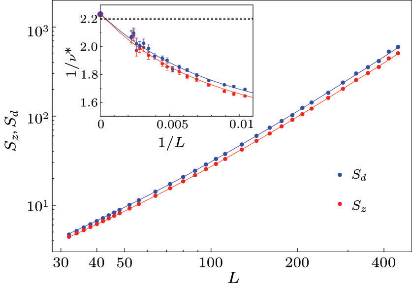
Fig. 4. Critical cumulant slopes vs the system size. The curves are fits of the L ≥ 64 data to the form aL1/ν(1 + bL−ω), with 1/ν = 2.23(2) (constrained to be the same for both data sets) and ω = 1.1(1) (for both data sets, not constrained to be the same). The inset shows 1/ν* ≡ ln[S(L)/S(L/2)]ln−1(2) vs 1/L. The purple circle indicates the extrapolated exponent 1/ν = 2.23(2) and the dashed lines show the values 1/ν = 3 – ΔQ = 2.200 ± 0.004 determined in Fig. 3.
Download figure:
Standard imageWhile the finite-size corrections in 1/ν obtained from the cumulant slopes in Fig. 4 are substantial, the corrections to the r−2ΔQ form of the correlation function in Fig. 3 are very small. The good agreement of the extracted exponents with the relationship 1/ν = 3 – ΔQ should alleviate any concerns of 1/ν eventually flowing to the value 3 ( = d) expected at a conventional first-order transition (or to d + 1, as found at an unconventional transition in Ref.[33]). Weak first-order transitions are often most clearly manifested in 1/ν,[51] and the results presented here simply do not indicate anything unusual.
Previously, anomalous scaling was found of the order parameters and the spin stiffness,[16,18,22,32] and it was argued that the standard finite-size scaling hypothesis must be replaced by a form taking into account two divergent length scales in a new way.[26] Though this interpretation has not been independently confirmed, the results presented here reinforce the notion that anomalies are not present in the magnitude L−1/ν of the critical window. The value ν=0.455(2) is still puzzling in the sense that it violates a CFT bound from the bootstrap method.[52] This disagreement suggests that the transition is either not described by a CFT or that the arguments underlying the bound have some loophole. It would be interesting to compute ν from the relevant critical correlator for fermionic DQCP candidate models,[53] where the standard finite-size analysis is difficult because of the rather small accessible lattices.
We would like to thank Jun Takahashi for useful discussions. The numerical calculations were carried out on the Shared Computing Cluster managed by Boston University's Research Computing Services.
Footnotes
- *
Supported by the National Science Foundation (USA) under Grant No. DMR-1710170 and by the Simons Foundation under a Simons Investigator Award.