
Abstract
The classification of grades inside a material family should be based on the properties required by design procedures. This paper proposes a reclassification of spheroidal graphite ferritic pearlitic and ausferritic (ADI) ductile cast irons grades based on yield strength (YS), strength ratio (SR) UTS/YS and elongation at fracture (EF). In fact, these parameters are fundamental for the static assessment according to the procedures FKM Guideline and BS 7910:2005. Static assessment at room temperature, involving plastic deformation and depending on the wall thickness and stress state triaxiality, is here proposed as the most significant for the material classification. All other properties (e.g., fatigue under cyclic loads, high strain rates and temperature effect, etc.) should be reported with reference to the classification mentioned above. SR and EF control the plastic deformation at the notch tip, where maximum calculated elastic stress is redistributed. Minimum YS is usually assumed as the basic parameter for static and cyclic loading design. Because of the inverse relationship that exists between strength and ductility, Brinell hardness control and material quality index should be adopted as Material Quality Control tools, preventing from a too low EF. Fracture Toughness and its ratio with YS must be considered for preventing brittle fracture due to the presence of flaws. Fracture toughness definitions and available data are not sufficiently consistent for a correct comparison between different material grades. A surrogate Charpy energy measurement is indicated for an indirect estimate of toughness.
Introduction
Spheroidal graphite cast irons (SGCIs) are a family of materials that compete favorably with steels for application in the manufacture of structural engineering components. The material family is featured by a microstructure that can be described as constituted by a “high-silicon steel matrix surrounding spheroidal carbon sinks.” Carbon sinks and silicon allow for solid-state heat treatment transformations that are not possible with steel. For example, the entire wall thickness can be transformed into carbon saturated austenite. During the liquid–solid transformation, carbon and silicon allow a much lower (compared with steel) melting temperature, self-feeding properties, a carbide-free matrix and protection against surface oxidation. On the other hand, graphite spheroids influence the plastic deformation of SGCIs under load after the onset of necking and/or even prevent the onset of necking to be met.
Because of its material characteristics, SGCIs are often evaluated as an alternative to cast, forged and welded steels. As a consequence, linear elastic strength parameters (yield strength, hardness, fatigue strength) are likely to be directly compared between SGCIs and steels. Ductility and toughness or the influence of material plastic and fracture properties on components design have not been sufficiently considered in existing material standard. This paper analyses the material properties information required by the design procedures for the assessment of components under static loads, to establish the main metrics for a proper reclassification of SGCIs Grades, in view of design needs.
Plastic properties after yielding are also important for the designer, and they are often empirically taken in consideration as an “a priori” material selection.
Reclassification Framework
The map in Fig. 1 shows different available processes, using yield strength-YS and strength ratio SR (UTS/YS) as coordinates. The map refers to a given general foundry process with particular focus on the manganese content. It is assumed that Mn is ≤ to 0.35%. Furthermore, separately cast test bars Y25 mm with a relevant wall thickness t ≤ 30 mm were used in the construction of this map.

Designation of SGCIs available processes
Design procedures take into consideration the SR and not the UTS Rm directly because the strength ratio (SR) = Rm/Rp0.2 is an immediate rough but reliable indicator of the material strain hardening behavior.
In Fig. 1, the ordinate SR is intentionally not scaled, because values depend on the base chemistry, foundry process, casting wall thickness, etc. The graph only provides a comparative image of the different processes.
Comparison with traditional specifications based on minimum properties Rp0.2 and Rm taken separately can be done by drawing a vertical line starting from the point (Rp0.2 min; Rm min/Rp0.2 min) and then connecting this point with (Rm min; 1). All points on the right conform to the minimum properties taken separately. By dividing the abscissa Rp0.2 into arbitrary intervals, we can classify materials into “Grades” (different Rp0.2 ranges with the lower value designating the grade) within a “Process.”
A material specification may comprise several adjacent grades belonging to the same process, depending on the acceptable variation of allowable hardness, machinability, and mechanical properties that can be obtained on the castings.
The terms “perlitizers/pearlite promoters” refer to elements (generally Cu and Sn) able to promote the formation of as-cast pearlite. The term “Alloying” refers to elements (generally Cu, Ni, Mo) able to displace the TTT and/or CCT heat treatment curves to the right side, promoting quenchability by avoiding the crossing of the pearlite nose.
Material Quality Index
Tensile tests conform to the present reclassification if the calculated “material quality index”15
with Rm in [MPa] and A5 in [1/100], is not lower than a minimum value that should be indicated for each grade.
In Fig. 2, values corresponding to Rm,min and A5,min of commercially significant grades are reported, including interpolations with indication of the reference source.Footnote 111,12,16,17,21 The actual MQI should always be higher, if the minimum specified properties are to be achieved, accounting for an allowable hardness (strength) scatter.

MQI of SGCIs available processes
Description of Material Manufacturing Processes
Structures Obtained in the As-Cast State and/or Heat Treated by Annealing
Process F Fully Ferritic Ductile Iron, with no Addition of Pearlite Promoters or Alloying Elements, Strength Increases with Si Content
Grades 220F, 240F, 260F, 300F in Fig. 1 align well with the traditional ISO 1083: 201816 grades (Rp0.2 min − Rm min) 220–350, 240–400, 250–400, 310–450 with increasing the silicon content from slightly below 2% up to slightly more than 3% which is a range generally considered as “normal” foundry practice.
Grades 340F, 380F, 420F, 480F align with ISO 1083: 2018 Silicon Solid Solution Strengthened Ferritic (SSSSF) grades 350–450, 400–500, 470–600.
Silicon contents equal to 3.2%, 3.8%, 4.2%, respectively, are suggested by ISO 1083: 2018 for SSSSF grades. The SSSSF concept should not be confused with high-silicon ductile irons for use at high temperatures.
Process F grades may require annealing, either in correspondence of a too low silicon content to dissolve carbides or in the correspondence of a too high manganese content to dissolve pearlite.
The first commercial practice of a SSSSF grade originated with the intent to fully recycle low-yield ductile iron casting returns: the addition of FeSiMg as the spherodizer would imply a silicon content greater than the typical “normal.” At this new (higher) silicon content, the yield strength Rp0.2 was found to be acceptable, compared with the requirements of the traditional ferritic–pearlitic grades 320–500 and 370–600 [MPa], even if the ultimate tensile strength Rm was insufficient to meet the material standard requirements.
In some commercial current practices, ferritic–pearlitic ductile irons are characterized by a wide variation in hardness within the casting and between castings, a fact that negatively affects machinability. The possibility to replace these irons with fully ferritic materials, characterized by a high level of uniformity in hardness and then in machining, appeared attractive for high volume automotive components and greatly contributed to the commercial success of this SSSSF approach. Consequently, the idea was further developed and extended to higher silicon contents in international material standards.
In addition to the hardness uniformity, a high post-necking elongation at fracture A5 is an attractive property of SSSSF grades. However, the decrease in the strength ratio and the negative effect of silicon content on the low-temperature behavior must also be considered. The risk of chunky graphite and its negative effect on fatigue strength and fracture toughness should also be of concern.6
Non-alloyed ferritic grades offer the best opportunity for uniform properties within the casting, allowing for design with the maximum geometric freedom. Silicon content (below 2% up to 4.2%) and heat treatment are the drivers for obtaining the different grades.
Low silicon contents are used for optimizing the ductility at low temperatures (up to − 40 °C), in the as-cast or annealed state. Normal silicon contents are of common use in the industrial practice in the as-cast state. High silicon contents (between 3.2 and 4.2%), in the as-cast state, are viewed as an opportunity to replace ferritic–pearlitic grades, avoiding potential hardness inhomogeneity.
Low and normal silicon spheroidal graphite cast iron grades are the most suited for obtaining sound castings. High silicon grades are more prone to formation of porosity and/or chunky graphite.
Process FP Pearlite Promoters Added to Modify the F–P Content
Pearlite promoters are added to ferritic grades 220F, 240F, 260F, 300F, to promote pearlite in the as-cast state.
Grades 300FP, 340FP, 380FP, 420FP match traditional ISO 1083: 2018 grades 320–500, 350–550, 370–600, 420–700 [MPa].
FP grades are of interest in design because they allow for increasing strength, therefore maintaining a high strength ratio. These grades are sensitive to the casting wall thickness, i.e., to the cooling rate in the mold which affects hardness, ductility and machinability. This is the reason why conventional standards require low values for the minimum elongation at fracture A5 (consider ISO1083/JS/600-3, 700-2, 800-2).
In FP grades, the addition of pearlite promoters is necessary. Pearlite and ferrite form in the solid state when carbon saturated austenite transforms during slow cooling. The transformation time is measured in hours and increases with wall thickness. In addition, the distance between spheroids (formed during solidification) increases with wall thickness. The resultant effect is segregation of pearlite promoting elements. Segregation increases with decreasing the cooling rate (or increasing the wall thickness), resulting in a reduction in ductility as well as non-uniform hardness in different section sizes of the casting.
Since the 1970s, the Fiat 52215 material standard12 has deviated from the approach of international material standards, by promoting ferritic–pearlitic spheroidal graphite cast irons based on hardness control and uniform wall thickness (consider Gh 60.38.10, Rm min 590 MPa Rp0.2 min 370 MPa A5 min 10%). As an evolution of the Fiat approach, more recent commercial evidence14 indicates the possibility that pearlite promoters are also added to the lower grades of SSSSF irons. Together with SSSSF grades, the hardness-controlled FP grades offer a solution to design needs by increasing strength while also maintaining good ductility. SSSSF and FP grades differ between each other because of the strength ratio and consequent plastic properties.
Structures Obtained After Quenching Into a Salt Bath
Process IDI7—Proeutectoid Ferrite and Pearlite from Intercritical Austenitizing Non-alloyed Iron Followed by Quenching Into a Salt Bath
If a non-alloyed ferritic grade is austenitized in the intercritical range AC1–AC3, a fraction of the matrix transforms from ferrite to austenite, while the remaining matrix remains as proeutectoid ferrite. Subsequent quenching into a salt bath transforms the austenite into pearlite. In Fig. 3, the microstructure evolution with different cooling rates is shown.

Possible microstructure evolution with different cooling rates
Although the heat treatment process of IDI appears similar to austempering, relevant differences distinguish the so-called Perferritic Isothermed Ductile Iron (IDI) from the Intercritical Ausferritic Austempered Ductile Iron (IADI).
The salt bath in the IDI process only plays a role to accelerate the cooling rate to execute an austenite-to-pearlite transformation above the martensite start temperature.
Hence, the properties of IDI are comparable to those of FP grades and not to those of IADI.
The advantage of IDI, when compared to FP is in the perferritic, instead of pearlitic–ferritic structure, and the perferritic microstructure is imposed by the higher cooling rate. The low carbon mobility at high cooling rates results in an interconnected structure which offers higher strength with a significant amount of proeutectoid ferrite. This, in turn, results in significantly higher ductility, Charpy impact energy and expected toughness. The absence of pearlite promoters results in pronounced uniformity of the matrix in different wall thicknesses.
In IDI, Si content can vary in the same range as in the Si-based ferritic grades. The lowest Si grades exhibit the best Charpy impact energy results, even at low temperatures (however not so good as upper ausferritic ADIs). Low and “normal” silicon contents can avoid the chunky graphite formation. By increasing the silicon content, strength increases and ductility decreases.
Process ADI-Ausferritic Spheroidal Graphite Irons (Austempered Ductile Iron—ADI)
ADI requires alloying to avoid the formation of pearlite during the heat treatment. The formation of pearlite in the as-cast state is a resultant consequence of this. The alloying policy in the ADI process has some degree of freedom for its optimization. In fact, alloying elements effective in the ADI process are:
-
Carbon (increasing the austenitizing temperature)
-
Manganese (segregates at the grain boundary)
-
Copper (segregates to the spheroid/matrix interface)
-
Nickel (segregates to the spheroid/matrix interface, but not as severely as Cu)
-
Molybdenum (segregates to the grain boundary)
The cast wall thickness (and uniformity) along with the design requirements will dictate the alloy content for the component which, in turn, drives the selection of the correct heat treatment temperatures and times. The heat treatment equipment (quench severity and capacity) also plays an important role in the production of a successful ADI casting
Designers will consider two advantages of ADI, in addition to its high strength level:
-
The brittle–ductile transition temperature of ADI is low because of the ausferritic structure;
-
The partial transformation of austenite into martensite (PITRAM, SITRAM effect) allows, in many cases, to avoid surface hardening treatments such as nitriding, induction or case hardening.
On the other hand, the ausferritic matrix limits the use of ADI at high temperatures.
The “Germanite” Mühlberger invention19 in the 1970s established two fundamental statements for the development of ADI technology:
-
1.
Where the Mn content is not greater than 0.3%, and the casting wall thickness is not larger than 100 mm, Mo is not a carbide stabilizer
-
2.
It makes sense to distinguish the ADI process into two separate items:
-
a.
Austenitization above the critical range (GGG 100 B/A)
-
i.
Austempering above the ausferritic nose (Upper ADI, shortly UADI)
-
ii.
Austempering below the ausferritic nose (Lower ADI, shortly LADI)
-
i.
-
b.
Austenitization inside the critical range (GGG 70 B/A) (Intercritical ADI, IADI)
-
a.
The designation of the two items comes from the German use (GGG for spheroidal cast iron) and from the ancient metric kgf/mm2, meaning B/A “Bainitic/Austenitic” as it was common to interpret the austempered structures in those times.
The process GGG 100 B/A is implemented through a Cu–Ni–Mo alloying content driven by the largest casting wall thickness and through a heat treatment cycle driven by the grade to be obtained.
The statement (1), permitting Mo as alloying element, reduces the necessity to use a high austenitizing temperature to increase hardenability. In this way, a shorter austempering time is allowed for which promotes austenite stability and, consequently, improves machinability.
The ADI process displayed in Fig. 1 (grades from 540 to 1140 ADI) includes the original GGG 100B/A M-Type Germanite process in addition to other chemistries such as molybdenum free and manganese content greater than 0.30%.
The process GGG 70 B/A, implemented through a Cu–Ni–Mo low alloying content (also using a low intercritical austenitizing temperature), is suitable for limited casting wall thicknesses.
Grade 480 M-Typ in Fig. 1 matches the original GGG 70 B/A Mühlberger patent.
The grade GGG 70 B/A attracted the interest of the American automotive industry, promoting the definition of the material grade AD 750 into the material standard SAE J2477: 2004, which advises that “…this grade will exhibit a microstructure containing some pro-eutectoidic ferrite…”.
The US Patent9 “Machinable austempered cast iron article having improved machinability, fatigue performance and resistance to environmental cracking,” essentially recalls the “Germanite/Mühlberger GGG 70 B/A” invention,19 claiming a preferred chemistry which substantially avoids or limits Mo alloying. Consequently, this material, commercially known as MADI (Machinable ADI), can be described as similar to the “Germanite/Mühlberger GGG 70 B/A” where the Mo content is claimed as lower than 0.20%. The chemistry limitation reduces the casting wall thickness able to be austempered with this process, compared with GGG 70 B/A. Data reported in10 based on chemistry Si 2.64% Mn 0.25% Cu 0.71% Ni 0.96% Mo = 0% are represented by the grade 480 MADI.
The inventors of MADI reported data from tests on resistance to environmental cracking:9 proeutectoid ferrite increases the resistance to environmental cracking in intercritically austenitized materials.
They also reported data on machining forces10 with the intercritically austenitized ADI being the most machinable of all grades of ADI.
The main advantage expected by selecting the ADI grades 480 M-Type and/or 480 MADI is the improved machinability, a direct consequence of the lower hardness. At the same time, better fatigue properties, compared with pearlitic ductile irons, along with impact resistance similar to the ferritic grades, are expected.
Manganese increases the carbon solubility into the primary austenite (opposite effect as in steels), while it decreases its solubility into the metastable austenite. Successful production of low grade ADIs is facilitated by low manganese content with carefully controlled austenitizing temperature, controlled chemical composition—austenitizing and austempering times—salt bath quenching capacity.
Among design properties, it is worth consideration that ADIs are favorite materials when high strain rates and/or low temperatures are of interest.20
Materials Properties of Interest in Structural Design
Mechanical structural components are often designed considering static and cyclic loadings, being the maximum equivalent stress not larger than the material YS Rp0.2.
However, this design process begins after the material grade has been selected.
If the material selection would be based only on YS, very few steel casting would be used for mechanical structural components. Steel forgings and welded fabrications would be considered in alternative to SGCI castings only considering economic issues and expected defects.
If a SGCI casting solution was adopted, for a given YS only one grade (see Fig. 1) would be candidate for Rp0.2 ≤ 300 MPa and/or Rp0.2 > 600 MPa. Among 300 and 600 MPa, more than one option exists. On the base of information available from material standards, it could be expected that the material selection would be based also upon elongation at fracture A5, Brinell hardness range, machinability, supply chain configuration, casting cost.
SSSSF grades from 300F to 480F would appear the most attractive to the designer in this range, also considering that Charpy test is sometimes claimed to be no more representative for design needs.
If design is based only on YS, why the EF A5 is important?
The MQI concept (see Fig. 2) helps the designer to control A5, while Fig. 1 advises that also the SR Rm/Rp0.2 is important.
And also the plane strain static fracture toughness KIC is important.
However, material standards are based on minimum values of UTS Rm, YS Rp0.2, EF A5, with no requirement for the SR Rm/Rp0.2 and for KIC.
YS, SR, EF, KIC are the design parameters necessary for controlling, with a simple linear elastic FEM calculation, the maximum overload a component is able to sustain without undergoing to failure initiation.
If the designer is confident on these properties, she/he will be able to design more extensively SGCI castings instead of steel components and, inside the SGCIs family, will be able to select more efficiently the most appropriate grade.
Discussion on Analytical Design Rules Against Overloading
It is not necessary to read this chapter and it is possible to go immediately to the chapter “Conclusions.”
This chapter is dedicated to those readers that are willing to understand and/or to give further contributes on how the above-mentioned material properties are connected with design rules in case of overloading assessment.
Analytical Strength Assessment of Components Technically Without Fault
In Fig. 4, all the possible states of tensile stress are represented with reference to the principal triad, being

Possible states of stress and strain in tension
The red line on the left is drawn assuming the coincidence between the middle and the minimum principal tension, while the black line on the right is drawn assuming coincidence between the middle and the maximum tension.
For a constant maximum principal, the minimum principal stress varies from
to
where CF3 is called “Constraints Factor of the Minimum Principal Stress,” being ν = 0.27 the Poisson ratio.
The Triaxiality Factor TF is calculated by dividing the mean hydrostatic stress by the von Mises equivalent stress.
On the bottom line of the diagram, we find the whole range of plane stress conditions (CF3 = 0, TF = 0.33 ÷ 0.67), from the uniaxial up to the symmetric biaxial state of stress. On the bottom line, the Von Mises equivalent stress is given by:
On the upper line of the diagram, we find the whole range of plane strain conditions (CF3 = 1, TF = 0.92 ÷ 1.84), where
On the left side (red line), it is defined as:
On the right side (black line), it is defined as:
As a rule of thumb, in plane stress σeq ~ σ1, while in plane strain σeq ~ ½ σ1. This helps in understanding how plane strain conditions contribute to stay far from yielding, promoting a linear elastic behavior.
In Fig. 4, the uniaxial test probe is associated with the state of stress TF = 0.33 and CF3 = 0, while three different blunt notched test probes having intermediate constraints factor are used for the measurement of the “strain at failure versus triaxiality factor.”
FKM Criterion for the Critical Strain
In FKM,13 we find the following criterion for the critical strain εertr:
where
Steels are defined as ductile materials, while SGCIs are defined as semi-ductile when A5 ≥ 6% and non-ductile when A5 < 6%. The attribute “ductile” for steel and “semi-ductile” for SGCIs depend on the post-necking behavior in the quasi-static uniaxial tensile test.
Common steels undergo pronounced restriction in area after the onset of necking, while ductile irons breaks before, or at, or after the onset of necking but, in any case, with a reduction in area not comparable with that characteristic of steels. This happens because of the spheroids.
How the different post-necking behavior contributes to different design properties is a complex issue that will not be considered in this discussion. Here, we simply observe how, for SGCIs, is possible to adopt two different approaches:
-
1.
Based on εref = 0.4 A5, FKM guidelines, conservative, see Fig. 5;
Figure 5 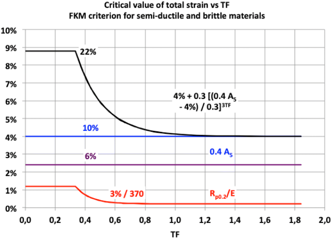
Critical value of total strain for semi-ductile and brittle materials (FKM)
-
2.
Based on εref = A5, non conservative, see Fig. 6.
Figure 6 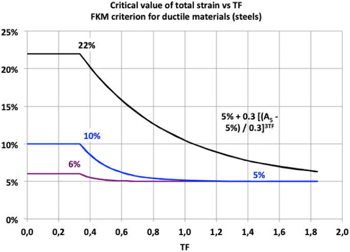
Critical value of total strain for ductile materials (steels) (FKM)


In any case, the beneficial effect of a high elongation at fracture A5 is amplified at low TFs (plane stress), as it happens on the smooth or blunt notched casting surface in the absence of flaws and of locally applied loads.
In20 an experimental determination of the strain at failure versus triaxiality factor is considered for an ADI cast iron.
In this case, the plastic true strain component pf is calculated, following the expression
where
and
(ν Poisson’s ratio, TF the triaxiality factor).
The true plastic strain in uniaxial tensile test was found to be εf = 14.45%, corresponding to the engineering value A5 = 16.34%.
The result is compliant with FKM criterion if approach (2) is adopted.
The FKM Double Criterion for the Critical Equivalent Stress
The critical equivalent stress at the reference point, otherwise stated as Component Static Strength, using local stress approach of FKM guidelines,13 in tension is given by
where npl is the double criterion section factor
The first term is the square root of the ratio between the total critical strain εertr and the elastic strain at yield Rp0.2/E.
The first criterion for σSK in tension
represents the maximum Neuber elastic peak applied to an ideally elastic perfectly plastic material model. Such a parameters can be assumed as “Ashby Material Index,”1 when evaluated at TF = 0.33, 0.67, 1.80, respectively.
The second term in (18) is the plastic notch factor, given by a material independent geometric coefficient, calculated using an elastic perfectly plastic material model (e.g., 1.5 for a rectangular section in bending) multiplied by
Multiplying by Rp0.2, we get the offset yield strength contributing to the net section yielding assessment
Rp,ers is also assumed as “Ashby Material Index.”
The proposed reclassification can then support the FKM static assessment using local stress approach with the following material properties, associated with each grade:
and the following material indices:
-
M1, M2, M3 critical strain maximum allowable Neuber elastic peak in tension, applied to an ideally elastic perfectly plastic material model at TF = 0.33, 0.67, 1.80;
-
M4 offset yield strength in tension, contributing to the net section yielding assessment by strain hardening.
Note that also A5 is a material property and that also MQI is a material index; however, they have no direct use in design but are used inside calculation steps for M1, M2, M3, which can be directly used in design.
For this, A5 and MQI are intentionally not classified as “Ashby Material Property” and “Ashby Material Index.”
The provided design material properties and indices enable to predict the initiation of a failure, but they will not provide any information on its possible evolution, which is the field of the assessment under cyclic loads and/or fracture mechanics and/or elastic–plastic analysis and/or other assessment criteria.
Design Needs Coming from BS 7910:20058 and Equivalent SINTAP and R6 Procedures: Acceptability of Flaws
We consider the static fracture mechanics approach applied to a cracked component characterized by a plane strain state of stress beyond the crack tip. The intent is to measure the Plane Strain Linear Elastic Fracture Toughness KIC material property, independent from the test probe, then directly applicable in design.
Some SGCIs grades (e.g., pearlitic, high-strength ADI) permit the direct measurement of KIC, compliant to ASTM E399, using a reasonable size CT test probe (e.g., taken from a Y50 [mm] test sample). Other grades (e.g., low-silicon ferritic, low-strength ADI) do not. Grades containing a significant amount of pro-eutectoidic ferrite at low/normal silicon contents require a J testing approach.
EN 1563:2018 Annex H11 advises: “With regard to the initiation of instable crack propagation under linear elastic conditions, fracture toughness values KIC in accordance with” ISO 12135:2016 and/or ASTM E399:2012 “are considered as transferable to the component.”
“The only characteristic material values to be considered as transferable to the component with regard to the initiation of crack propagation under elastic–plastic conditions are physical crack initiation toughness values (e.g., Ji in accordance with ISO 12135) excluding any crack growth. The characteristic crack initiation toughness value JIc according to ASTM E 1820 contains considerable amounts of ductile tearing and does not fulfill the above condition unless additional validity requirements are met.”
Baer5 also advises: “As has been shown for Ductile Cast Irons, the value of elastic–plastic fracture mechanics crack initiation toughness may vary up to 60% even when the same set of data is analyzed simply using different definitions from different editions of several ASTM and ISO test standards.”
When a valid Ji (J integral at crack growth initiation) is available, it can be converted, under plane strain conditions, into
to be used with the same meaning of KIC.
We suggest describing this possibility using the following sentences: “The actual test probe cannot behave under linear elastic conditions with the material under examination. If the test probe would change according to the linear elastic requirements, then a valid KIC ≈ KJI would be measured.”
EN 1563:2018 Annex H11 advises: “As far as performing fracture mechanical assessments on spheroidal graphite cast iron components is concerned, compilations of engineering rules and regulations such as the British Standard BS 7910 or the European FITNET procedure are available.” The aforementioned regulations are based on the Failure Assessment Diagram (FAD).
Consider a sharply notched generic component, loaded with a generic load pattern P, with the material behaving in a perfectly linear elastic way. Assume that the component is also cracked at the notch tip and that the crack opens in Mode I. The stress intensity factor (SIF) KI is proportional to the load P and tables or linear elastic FEM analysis gives the constant of proportionality. It is of common use to write the proportional relationship in the form
where KI (P) is the calculated SIF and σref (P) is an arbitrary chosen reference stress, also proportional to P.
The “equivalent crack length” is simply calculated from
and it is a constant characteristic of the component geometry, loading pattern, reference stress definition, but independent from the load P intensity.
From:22
“Whereas there is only a single KI solution, the limit load,” then σref, “depends on whether the specimen is in plane stress or plane strain” then, generally speaking, on the state of stress, “and on whether the von Mises or Tresca yield criterion is adopted” then, generally speaking, on the yield criterion.
We assume here that σref is always defined with reference to plane strain state of stress and von Mises yielding criterion.
If σref is defined (using available formulas for standard geometries and/or, generally, by linear elastic FEM analysis) following a criterion of yielding concurrent with the crack growth initiation, then the formulas (23) and/or (24) can be seen as a prediction of the crack growth initiation based on the simple calculation of the linear elastic SIF. For a given linear elastic proportional loading pattern α2a, the point (σref; KI) corresponds to the crack growth initiation on the failure assessment line.
For those loading patterns to which LEFM applies, the Failure Assessment Line (initiation of crack propagation) becomes
where \( \sigma_{\text{ref}}^{i} \) is the reference stress at the crack growth initiation.
In static assessment, LEFM applies only if “the plastic zone size ahead of the crack tip is ‘small’ compared to the crack size, say for example four times smaller.4 Under this hypothesis, the plastic zone size Rp can be estimated from Irwin’s linear elastic equations and is given by:
where y equals 1 for plane stress and 3 for plane strain conditions and σs is the material yield stress.”4
Assuming plane strain conditions and σs = Rp0.2, LEFM Failure Assessment Line applies when
At lower equivalent crack lengths, EPFM applies. This means that, instead of (25), the following equation appliesFootnote 2:
where N = 1/n is the power law exponent in the Ramberg–Osgood constitutive law
being n the strain hardening exponent in the Hollomon equation
The strain hardening exponent n is assumed as given by an empirical lower bound value
as suggested in the literature2,8,22
The meaning of Eq. (28) is that, when the plastic zone beyond the crack tip is large (EPFM), the linear elastically calculated SIF (right side of the equation) at crack growth initiation is lower than KIC. The reduction factor (multiplier of KIC on the left side) depends on:
-
The strain hardening exponent n and/or the Ramberg–Osgood power law exponent N = 1/n;
-
The \( \left( {\frac{{K_{\text{IC}} }}{{R_{p0.2} }}} \right)^{2} \) material characteristic length;
-
The geometric linear elastic crack equivalent length α2a.
The amount of the reduction is predictable, and then it is sufficient for a linear elastic analysis for calculating the load at crack growth initiation under linear elastic plane strain state of stress, even when the component behaves in EPFM mode beyond the crack tip.
Both LEFM and EPFM crack growth initiation lines can be regarded as
condition.
The failure assessment line is represented in Fig. 7.

Static Kitagawa diagram
For α2a ≥ a0EP, LEFM is dominant and the failure assessment line is given by (25).
For α2a < a0EP, EPFM is dominant and the failure assessment line is given by (28) until the reference stress is smaller than the offset yield strength.
As the load linear elastically increases the computation of the reference stress on the CDE line, we have in D a SIF = KI < KIC in correspondence of which the crack growth initiates. This happens because the elasto-plastic energy in the plastic process zone reaches the material critical value Ji.
Rewriting (28)
Rearranging (27)
then
and finallyFootnote 3
We get an equivalent form of the EPFM line, linking the linear elastic relative SIF at the crack growth initiation
to the linear elastic relative reference stress at the crack growth initiation
The change of coordinates is graphically represented in Fig. 8.

Static Kitagawa diagram—coordinates change for FAD
Figure 9 shows FADs at crack growth initiation compliant with BS 7910:20058 Level 2B (and equivalent SINTAP and R6 procedures), where the relationship between Kr and Lr in plane strain is given by
of possible evaluation when the material properties yield strength (P1) and
and Material Index
enable the Ramberg–Osgood constitutive curve to be drawn.

FAD as in BS 7910: 2005 Level 2B
Two potential collapse modes are identified (BS 7910:20058 Annex P):
-
Collapse of the remaining ligament adjacent to the flaw being assessed—local collapse;
-
Collapse of the structural section containing the flaw—net section collapse.
Collapse of the structure by gross straining—gross section collapse, when collapse takes place away from the flawed section or is unaffected by the presence of the flaw, is not considered by FAD.8
The “reference stress” σref is the stress used for plastic collapse considerations.8
Annex P (normative) of BS 7910:20058 provides formulae for the calculation of σref for local and/or net section collapse for various structural configurations, as a function of the applied load.
Lr, the ratio of the applied load to the yield load, is a measure of the amount of plasticity at the crack tip and shall be limited to a maximum value called “flow stress” or “effective yield after strain hardening”:8
M6 is an “Ashby Material Index” distinct from M4, being the latter subjected to a threshold value for the strength ratio.
For most applications, it is acceptable to use engineering stress–strain data, but it is important to concentrate calculation points around Rp0.2:
Lr = 0.7–0.9–0.98–1.0–1.02–1.1–1.2 and intervals of 0.1 up to the “effective yield.”8
Spheroidal graphite materials grades show yield ratios varying in a range as
and/or
hence
In Fig. 9, the two extreme constitutive curves (42), component independent, are drawn.
The loading pattern of a cracked component, subjected to an applied primary (contributing to yielding) load, is represented by a point (Lr, Kr) positioned on a straight line originated in (0, 0) featured by slope:
The slope is given by the contribution of two terms:
-
KI/σref, linear elastically representing geometry, crack, load, assuming plane strain state of stress and von Mises criterion, material independent, and corresponding to the effective crack length α2a in the Kitagawa diagram;
-
Rp0.2/KIC, material contribution corresponding in the Kitagawa diagram to a0EP, the transition crack length from EPFM and LEFM.
Rearranging (43), the following relation can be obtained:
We define as “Slope Factor” SF the ratio between the “Material Characteristic Length” (material index)
and the “Effective Crack Length” α2a.
Let us compare two materials, representing the whole range of SGCIs grades, having any Rp0.2 and any KIC, but different strain hardening exponents n, and consequently different Ramberg–Osgood power law exponents
with
and with
In Fig. 9, the black and red thick continuous lines are drawn by (36), while the thin ones are drawn considering only the first term (see23).
In Fig. 9, the loading pattern SF = 0.35 ÷ 0.51 (values depending only on W/a) corresponds to the compliance condition 2.5 (KIC/Rp0.2)2 for the minimum ligament W–a in ASTM E399 of a CT specimen.
This result is obtained from the rearranged SINTAP22 equations for an ASTM E399 CT specimen
Equation (46) gives approximately the same results as ASTM formulas3
when a/W is in the range 0.4 ÷ 0.7. ASTM does not indicate any expression for the reference stress.
The constitutive ratio KI/σref, in plane strain conditions and using the von Mises yielding criterion, depends only on the crack depth a and ligament ratio a/W and thus derives by a bi-dimensional model.
The loading pattern SF = 2.4 (a constant for all materials) corresponds to the transition between LEFM and EPFM, following the schematic Kitagawa diagram4.
The EPFM regime lasts until the load reaches the value σref = Rp0.2, at a SF depending on the material index Rp0.2/E.
This material index is not of interest when selecting a material within the SGCIs family, but it is of interest when the selection is done between SGCIs grades and other material families, such as steels and/or aluminum alloys.
SGCIs considered in this paper can be loaded at σref = Rp0.2 (plane strain crack growth initiation) at SF ranging from a value of 9 for low silicon ferritic DI and 5 for high strength ADI.
At lower equivalent crack lengths, the load could be larger than yield before the plane strain crack growth initiation (PYFM, Post Yield Fracture Mechanics), up to the maximum cutoff value Lr maxRp0.2.
The maximum value is reached when the loading pattern SF crosses the FAD curve at Lr max, SF value depending on M8 and M5:
Charpy Test and Plane Strain Fracture Toughness
For a number of years, SGCIs standardization WGs have debated the adoption of the Charpy test inside the material standards. Casting manufactures are concerned that the comparison of Charpy energy values between SGCIs and steels will discourage potential SGCIs casting applications. On the other side, designers that are interested to change material are afraid of unexpected material behaviors, even considering they are not using Charpy values in their calculation codes.
It has been proposed18 that the difference in Charpy energy between the two material families consists in the “shear lips advantage” of steels, undergoing a plane stress state of stress at the external surfaces of the test probe.
From the concept,18 it can be indicated that the main difference between SGCIs and steels is in the post-necking behavior, when common steels show pronounced restriction in area, while SGCIs do not because of spheroids. The material behavior in the post-necking regime is a complicated issue. Its description requires complicated and non-standard approaches based on damage models. This field of investigation is not comprised in the scope neither of this paper nor of the here considered design guidelines; both consider the material behavior up to the damage initiation not exceeding the offset yield strength, where the uniform nonlinear deformation of the quasi-static tensile test constitutive curve applies.
The Charpy V-notch energy value, at a given temperature, is determined by the concurrent contribution of the following material properties:
-
Shear lips advantage/post-necking behavior;
-
Strain rate sensitivity;
-
Fracture toughness.
For steels, correlations are proposed between Charpy V-notched energy values and fracture toughness.
“Where Charpy results are available at the temperature at which Kmat is required, the following equation can be used to estimate fracture toughness:8
where Kmat is the estimate of the fracture toughness in MPa√m, B is the thickness of the material for which an estimate of Kmat is required (in mm), CV is the lower bound Charpy V-notch impact energy at the service temperature (in joules).”
Martinez et al.18 proposed also for ADIs a linear correlation between the Material Characteristic Crack Length (KIC/Rp0.2)2 in [mm] and (CV/Rp0.2) or (CU/Rp0.2) in [J/MPa], where CV stays for V-notched Charpy and CU for Un-notched Charpy.Footnote 4
Equation (53) is in good agreement with the data of ISO 17804, using for Rp0.2 the minimum value specified for the grade (see Table 1).
Figure 10 shows the trend lines of V-notched Charpy energy values of SGCIs tested at Zanardi Fonderie laboratory, specimens taken from Y50 [mm] test samples, convenient for fracture toughness testing. Thick lines are related to RT, dotted lines to − 20 °C, and pointed lines to − 40 °C. For FP (red lines), − 20 and − 40 °C lines are coincident. IDILT (low silicon, low temperature) and IDIRT (normal silicon, room temperature) are considered at one average Rp0.2 value. The highest dot is at RT, the lowest dot is at − 40 °C.

Trend lines for V-notched Charpy energy values
Figure 11 converts the CV data of Fig. 10 into Fracture Toughness data KJIC, using the trend line of the Wallin equation for SGCIs24

Fracture toughness estimated by conversion of V-notched Charpy energy
Values from actual or obsolete material standards are also reported in Fig. 11.
Wallin fundamental indications are:
-
SGCIs should have the same correlation between Charpy V and fracture toughness in both the transition and the upper shelf region;
-
It is possible to estimate an equivalent impact energy that gives the same fracture toughness for steel as for SGCIs.
Defining Wallin Steel Equivalent Charpy V-notch WSECV, the impact energy of a steel having the same fracture toughness of a SGCI having a given Charpy V-notch impact energy CV, we get from Table 1 in24 the following best fit correlation
Note that (55) matches (52), where CV is substituted by WSECV assuming B ≈ 7 mm which is closed to the 10 × 10 mm size of the standard Charpy specimen.
Two new material properties have to be defined
together with a new material index
Real Cracked Components
The acceptability of flaws using the FAD has been described considering a reference stress calculated in plane strain conditions and also using a plain strain toughness material property KIC.
The designers (and the component design standards) are also interested to know the grade of safety offered by different materials, in case the essentially linear elastic design and plane strain based calculations are violated on the field. In simple words, the materials’ “forgiveness ability” is of interest.
These kinds of evaluation cannot be referred to the material only but have to consider also the component geometry and loading pattern.
Conclusions
A cube {ΔYS; ΔSR; ΔMQI} of appropriate size on the three dimensions is proposed as identifier of one SGCI grade at the minimum granularity. ΔYS granularity level is defined as in Fig. 1, for ΔSR and ΔMQI it depends on the foundry process capability.
Measured material properties and calculated material indexes, to be used in components design, should be associated with a cube at the minimum granularity, and the position identified in this cube can be used to synthetically identify the mechanical properties of a specific SGCI.
The following material properties and material indexes are of immediate use in design, after a linear elastic FEM has been performed:
Material Properties
- P 1 :
-
Yield strength: Rp0.2
- P 2 :
-
Strength ratio: Rm/Rp0.2
- P 3 :
-
Young’s modulus: E
- P 4 :
-
Plane strain linear elastic fracture toughness: KIC or KjI
- P 5 :
-
Un-notched Charpy energy value: CU (estimate of P4 at different temperatures)
- P 6 :
-
V-notched Charpy energy value: CV (estimate of P4 at different temperatures)
- P 7 :
-
Fatigue strength on a smooth specimen (stress and/or strain controlled)
- P 8 :
-
Fatigue strength on sharply notched/cracked specimen (stress controlled)
Material Indexes
- M 1 :
-
Critical strain maximum allowable Neuber elastic peak in tension, applied to an ideally elastic perfectly plastic material model at TF = 0.33: σSK 1st criterion
- M 2 :
-
Same at TF = 0.67
- M 3 :
-
Same at TF = 1.80
- M 4 :
-
Offset yield strength in tension with threshold P2 ≥ 1.33: Rp,ers
- M 5 :
-
Power law exponent in Ramberg–Osgood constitutive equation: N
- M 6 :
-
Relative offset yield strength in tension without threshold: Lr max
- M 7 :
-
Material characteristic crack length: (KIC/Rp0.2)2
- M 8 :
-
Yield-to-stiffness ratio: Rp0.2/E
- M 9 :
-
Wallin steel equivalent Charpy V-notched energy value: WSECV
Materials properties available from the quasi-static uniaxial tensile test are essentially the Young’s modulus E, the yield strength Rp0.2, the ultimate tensile strength Rm and the elongation at Fracture A5.
Plane strain linear elastic fracture toughness KIC should be measured whenever possible following ASTM E399 requirements, using a test probe taken from a representative test sample (e.g., Y50 [mm]).
When the material ductility is too high for the ASTM E399 requirements, a substitute KjI should be converted from a valid physical crack initiation toughness value (e.g., Ji in accordance with ISO 12135) excluding any crack growth.
For material selection purposes only, the adoption of a substitute Wallin Steel Equivalent Charpy V-notched Energy Value WSECV is proposed.
For material standard normative purposes, the elongation at fracture A5 is considered not directly but as a component of the material quality index MQI, in this way avoiding indeterminateness due to the inverse statistical relationship between Rm and A5.15
The Ultimate Tensile Strength Rm is considered not directly but as a component of the strength ratio (SR), in this way characterizing the manufacturing process and consequently the material properties for design.
In design, the calculated
does not enter directly in calculations, being a component of the “strain at failure versus triaxiality factor,” calculated using a standard threshold value at high triaxiality.
Contractual Specifications
Regarding contractual design specifications the following procedure should be recommended:
1. Specify, at given locations on the castings, the minimum and maximum hardness HBWmin and HBWmax; |
2. For the actual DI material process and for different thicknesses Y25 Y50 Y75 [mm] calculate the relationships between Rm and Rp0.2 versus HBW (see EN 1564:2011 Annex E, ISO 17804:2005 Annex D); |
3. Calculate Rm min, Rm max, Rp0.2 min, Rp0.2 max using the correlations established at point 2: |
a. \( R_{m} = A*{\text{HBW}} + B \) (Eq. 56) |
b. \( R_{p0.2} = \, C*{\text{HBW}} + D \) (Eq. 57) |
4. Specify the separately cast test sample Y25 Y50 Y75 [mm] and/or the casting best sounda location where to cut the tensile test specimen. The Brinell hardness measured on the tensile test specimen should be found inside the range HBWmin ÷ HBWmax; |
5. Specify the minimum MQI to be obtained from the tensile test. |
The strength ratio (SR) = Rm/Rp0.2 versus HBW is monotonous, then
SRmin makes the designer confident versus the FKM offset yield strength Rp, ers (21) and versus the FAD maximum ratio of the applied load to the yield load Lr max (38).
The first criterion for σSK (19) is controlled by
The ratio (R2m /Rp0.2) versus HBW is growing monotonous, then
Equation (59) makes the designer confident versus the FKM critical strain criterion.
Figures 12 and 13 show an example of design confidence based on contractual specification.

Relationship between hardness and strength for traditional F FP SGCIs

FKM component static strength critical strain control using MQI specification
Traditional ferritic (excluding high silicon) and ferritic pearlitic grades are considered.
Specifying the HBW range, the designer is confident on the Rm and Rp0.2 ranges and also on the strength ratio (SR) that we can see is not significantly changing in the whole interval being even more uniform in the specified HBW range.
For the required material quality index (MQI), the minimum elongation A5 at the right end of the interval is 64% of the maximum elongation at the left end. But the minimum value controlling the Component Strength limited by the Critical Strain is 89% of the maximum.
One can observe that, from a design point of view, it would be more convenient to directly specify a (Rp0.2A5)min requirement. But this is not the case, because the statistical output of a given foundry process is best described by a relationship (Rem A5) = const and not by (Rfp0.2 A5) = const. It can also be observed that Rm and A5 are close events, while Rp0.2 and A5 are nearly independent events in the uniaxial tensile test flow curve.
Notes
ZAN = Zanardi Fonderie.
Equation (28) comes from the exponent − 1/(N + 1) for the EPFM logarithmic line and from the intersection of EPFM with the LEFM line at the abscissa a0EP.
\( K_{r} = \left( {\frac{1}{4}} \right)^{{\frac{N - 1}{4}}} L_{r}^{{ - \frac{N - 1}{2}}} \) in plane stress.
In the original paper18, an inversion between notched and un-notched is wrongly done.
A plastic spot is a location stressed above the yield strength, completely surrounded by material stressed in linear elastic condition.
References
M.F. Ashby, Materials Selection in Mechanical Design, 3rd edn. (Elsevier, Amsterdam, 2005). ISBN 0-7506-6168-2
ASM HANDBOOK, Fatigue and Fracture, vol. 19, Fifth printing October 2007 (ASM International, 1996). https://doi.org/10.31399/asm.hb.v19.9781627081931
ASTM E399-09, Standard Test Method for Linear-Elastic Plane-Strain Fracture Toughness K Ic of Metallic Materials (ASTM International, West Conshohocken, PA, 2009). www.astm.org, https://doi.org/10.1520/E0399-09
B. Atzori, G. Meneghetti, Static Strength of Notched and Cracked Components, Proceedings of the 5th International Conference New Trends in Fatigue and Fracture 5 NTFF5, Department of Mechanical Engineering, University of Padova, Bari, Italy, May 2005
W. Baer, Advanced fracture mechanics testing of DCI—a key to valuable toughness data. Int Metalcast 8, 25–34 (2014). https://doi.org/10.1007/BF03355579
W. Baer, Chunky graphite in ferritic spheroidal graphite cast iron: formation, prevention, characterization, impact on properties: an overview. Int Metalcast (2019). https://doi.org/10.1007/s40962-019-00363-8
M. Bronzato, Z. Ilibasic, F. Zanardi, Method for manufacturing spheroidal cast iron mechanical components (IDI), EP 2 038 435 B1, ZL200780025272.5, U.S. Patent 8,328,965 B2, 11 Dec 2012
BS 7910:2005, Guide to Methods for Assessing the Acceptability of Flaws in Metallic Structures. ISBN 0 580 45965 9
Druschitz et al., U.S. Patent 7,497,915, 3 Mar 2009 (MADI)
A. Druschitz, M. Ostrander, R. Aristizabal, The Science of Intercritically Austempered Ductile Iron (IADI), The 71st World Foundry Congress Bilbao, Spain, Paper #22 (2014)
European Standard EN 1563:2018 (E), Founding—Spheroidal Graphite Cast Irons, ICS 77.080.10
Fiat Auto Normazione, Ghisa a grafite sferoidale—Norma materiali 52215
FKM Guideline, Analytical Strength Assessment of Components Made of Steel, Cast Iron and Aluminum Materials in Mechanical Engineering, 6th edn. (VDMA Verlag, 2012)
H. Stefan, Lightweight by bionic design approach, Georg Fischer Automotive (2014)
ISO/TC 25/SC 2/WG 1 Richard Gast and Franco Zanardi, Procedure for the adoption of a Material Quality Index (2001)
International Standard ISO 1083 : 2018 (E), Spheroidal Graphite Cast Iron—Classification
International standard ISO 17804 : 2005 (E), Founding—Ausferritic Spheroidal Graphite Cast Irons—Classification
R.A. Martinez, R.E. Boeri, J.A. Sikora, Impact and fracture properties of ADI, compared with SAE 4140 steel. T Am Foundrymen’s Soc 106, 27–30 (1998)
H. Mühlberger et al., Cast Iron with Spheroidal Graphite and Austenitic-Bainitic Mixed Structure, U.S. Patent 4,541,878, 17 Sept 1985 (ADI)
A. Ruggiero, G. Iannitti, S. Masaggia, F. Vettore, ADI 1050-6 mechanical behavior at different strain rates and temperatures. Mater Sci Forum 925, 196–202 (2018). https://doi.org/10.4028/www.scientific.net/msf.925.196
SAE J2477, Automotive Austempered Ductile (Nodular)Iron Castings (ADI)
SINTAP Procedure Final Version November 1999
Smith Simon, TWI Ltd., Development of the BS 7910 Failure Assessment Diagram for Strain Based Design with application to Pipelines. Proceedings of the ASME 2012 31st International Conference on Ocean, Offshore and Arctic Engineering OMAE 2012 July 1-6 2012, Rio de Janeiro, Brazil
K.R.W. Wallin, Equivalent Charpy-V impact criteria for nodular cast iron. Int Metalcast 8, 81–86 (2014). https://doi.org/10.1007/BF03355584
Acknowledgements
Thank you to Dr. PhD Kathy Hayrynen for her kind and competent help in advising and reviewing the text.
Author information
Authors and Affiliations
Corresponding author
Additional information
Publisher's Note
Springer Nature remains neutral with regard to jurisdictional claims in published maps and institutional affiliations.
This paper is an invited submission to IJMC selected from presentations at the 2nd Carl Loper 2019 Cast Iron Symposium held September 30 to October 1, 2019, in Bilbao, Spain.
Disclaimer: The present paper is not a direct design support. Its purpose is to make the case for improving material standards for spheroidal graphite cast irons (SGCIs) to address the true needs for designing with these materials. The work is the result of a collection about the material characterization performed by Zanardi Fonderie in cooperation with connected research centers that have worked on material samples supplied by Zanardi Fonderie.
Appendices
Appendix
This Appendix provides numerical examples of possible design problems for which the described concepts can be used. It can be also used for a better understanding of the concepts in this paper by using numerical examples.
Problem A
Description
An analytical static strength material comparative loading capacity at room temperature is required, following FKM guidelines, in order to calculate the maximum allowable von Mises equivalent stress at a geometrical notch root for five different tested materials (Fig. 1): 300F, 480F, 480IDI, 420FP, 780ADI for three different thicknesses: Y25, Y50, Y75 [mm] and in correspondence of three different triaxiality factors TF: 0.33, 0.67, 1.80. Evaluate the case if the assessment point is or is not a plastic spot.Footnote 5
The quasi-static tensile test mechanical properties are listed in the following table.

Calculations and Discussion
The elongation A5 for 420FP in Y50 and Y75 and 780 ADI in Y75 is lower than the threshold value 6% (12) (13). The εref, proportional to A5, is calculated (11) in row 1 assuming an identical value (170 GPa) for all materials for Young’s modulus. The critical strain at high triaxiality εth is calculated (12) (13) in row 2.
Finally, the critical strain εertr at three different triaxiality factors TF is calculated (9) (10) in rows 3, 4, 5.
300F | 480F | 480IDI | |||||||||
|---|---|---|---|---|---|---|---|---|---|---|---|
Y25 | Y50 | Y75 | Y25 | Y50 | Y75 | Y25 | Y50 | Y75 | |||
1 | εref | 10.1% | 10.4% | 8.2% | 5.6% | 5.2% | 4.0% | 3.6% | 3.8% | 3.4% | |
2 | εth | 4.0% | 4.0% | 4.0% | 4.0% | 4.0% | 4.0% | 4.0% | 4.0% | 4.0% | |
3 | εertr | TF = 0.33 | 10.1% | 10.4% | 8.2% | 5.6% | 5.2% | 4.0% | 3.6% | 3.8% | 3.4% |
4 | εertr | TF = 0.67 | 5.2% | 5.4% | 4.6% | 4.1% | 4.0% | 4.0% | 3.6% | 3.8% | 3.4% |
5 | εertr | TF = 1.80 | 4.0% | 4.0% | 4.0% | 4.0% | 4.0% | 4.0% | 3.6% | 3.8% | 3.4% |
420FP | 780ADI | |||||||
|---|---|---|---|---|---|---|---|---|
Y25 | Y50 | Y75 | Y25 | Y50 | Y75 | |||
1 | εref | 3.0% | 1.9% | 1.6% | 5.3% | 3.2% | 2.1% | |
2 | εth | 4.0% | 0.2% | 0.2% | 4.0% | 4.0% | 0.5% | |
3 | εertr | TF = 0.33 | 3.0% | 1.9% | 1.6% | 5.3% | 3.2% | 2.1% |
4 | εertr | TF = 0.67 | 3.0% | 0.3% | 0.3% | 4.1% | 3.2% | 0.6% |
5 | εertr | TF = 1.80 | 3.0% | 0.2% | 0.2% | 4.0% | 3.3% | 0.5% |
In the case of plastic spot, only the critical strain controls the local failure. The maximum load is defined as the Neuber elastic peak M1, M2, M3 obtained by multiplying the critical strain by the YS (rows 6, 7, 8).

Unalloyed materials (F and IDI) show more uniform behavior at different thicknesses than alloyed materials.
The maximum allowable linear elastic stress peak by critical strain (M1, M2, M3) is compared with the offset yield strength contributing to the net section yielding (M4), which, in turn, depends on yield strength Rp0.2 and the strength ratio P2. The geometric plastic notch factor Kp* is calculated in correspondence of which the two stresses are identical. If the actual geometric plastic notch factor is larger than Kp*, then the component will locally fail by critical strain; otherwise, it will fail by net section yielding.
Commonly, geometric plastic notch factors range between 1.0 and 1.7.

This demonstrates when the tensile state of stress is not uniaxial, FP DIs Y50 and Y75 and ADI Y75 locally fail by critical strain instead of net section yielding.
The M4 parameter is displayed in the following diagram for materials and thicknesses failing by net section yielding.

Unalloyed materials (300F, 480F, 480IDI) fail by net section yielding on the three wall thicknesses (Y25, Y50, Y75), while alloyed materials miss this opportunity on the heaviest sections (FP on Y50 and Y75, ADI on Y75). At the YS level 480 MPa, 480IDI allows a maximum stress 1/3 higher than 480F.
Problem B
Description
For the same materials described in Problem A, evaluate the acceptability of flaws at RT. For this assessment, the elongation at fracture is not needed. Calculations with reference only to one wall thickness (Y50) are assumed to be significant.
The quasi-static tensile test needed mechanical properties at RT are shown again in the following table.
NO ALLOYING | ALLOYING | |||||
|---|---|---|---|---|---|---|
AS CAST | AS CAST | HEAT TREAT. | AS CAST | HEAT TREAT. | ||
300F | 480F | 480IDI | 420FP | 780ADI | ||
Y50 | Y50 | Y50 | Y50 | Y50 | ||
Rm | MPa | 429 | 615 | 826 | 680 | 1068 |
Rp0.2 | MPa | 300 | 504 | 515 | 423 | 790 |
Calculations and Discussion
Rows from 1 to 5 calculate the parameters needed for drafting the failure assessment line (FAL).
300F | 480F | 480IDI | 420FP | 780ADI | |||
|---|---|---|---|---|---|---|---|
Y50 | Y50 | Y50 | Y50 | Y50 | |||
Rm | MPa | 429 | 615 | 826 | 680 | 1068 | |
Rp0.2 | MPa | 300 | 504 | 515 | 423 | 790 | |
1 | P1 | MPa | 300 | 504 | 515 | 423 | 790 |
2 | M5 | 11 | 18 | 9 | 9 | 13 | |
3 | K | MPa | 526 | 706 | 1039 | 856 | 1283 |
4 | E | GPa | 170 | 170 | 170 | 170 | 170 |
5 | M6 | 1.22 | 1.11 | 1.30 | 1.30 | 1.18 |
-
Row 1: P1 = Rp0.2;
-
Row 2: M5 = N power law exponent in Ramberg–Osgood constitutive Eqs. (31) (37);
-
Raw 3: K = Rp0.2/(0.2%)1/N strength coefficient in Ramberg–Osgood constitutive Eq. (29);
-
Raw 4: E Young’s modulus
-
Row 5: M6 = Lr max relative offset yield strength (38).
The FALs for the five materials can then be calculated using (29) and (36), with no need to know any fracture toughness parameters, only the usual parameters from the quasi-static uniaxial tensile test.

It is evident the difference between materials containing a significant amount of proeutectoid low-normal silicon ferrite (300F, 420FP, 480IDI) and materials not containing proeutectoid ferrite (780ADI) or whose matrix is silicon solid solution strengthened ferrite (SSSSF). From a mechanical point of view, the FAL shape is a direct consequence of the strength ratio (SR) (Fig. 1).
Considering this aspect, the designer can select the most appropriate material for an actual component.
The material fracture toughness parameters are then evaluated.
300F | 480F | 480IDI | 420FP | 780ADI | |||
|---|---|---|---|---|---|---|---|
Y50 | Y50 | Y50 | Y50 | Y50 | |||
6 | P6 | J | 16.4 | 2.2 | 6.6 | 2.8 | 10.1 |
7 | P4 | Mpa m0.5 | 87 | 39 | 61 | 43 | 72 |
8 | M7 | mm | 85 | 6 | 14 | 10 | 8 |
-
Row 6: P6 = CV estimated as a function of P1 = Rp0.2 following the trend lines in Fig. 10;
-
Row 7: P4 = KIC or KjI fracture toughness estimated by conversion of V-notched Charpy energy P6 using Wallin Eq. (55) displayed in Fig. 11;
-
Row 8: M7 = (KIC or KjI /Rp0.2)2 material characteristic crack length (45).
The fracture toughness of the ferritic grade 300F in row 7, calculated from Charpy value, is aligned with a J conversion into KjI and could not correspond to a Small Scale Yielding requirement, while the toughness values of the other materials are more compatible with valid KIC values. For this, the grade 300F results have to be regarded of qualitative practical interest, even not quantitatively comparable with the other grades. The index M7 represents the material contribution to the slope of the linear pattern of primary loads (contributing to yielding) using a linear elastic fracture mechanics (LEFM) approach. Increasing M7 increases the ductile behavior at the crack growth initiation. In other words, for a given crack size with increasing M7, the size of the plastic volume at the crack tip increases and the behavior at the crack growth initiation is displaced toward an effective elasto-plastic fracture mechanics model (EPFM).

The “equivalent crack length ECL” α2a (24) represents the component geometric contribution to the linear pattern of primary loads using a LEFM model. ECL could also be used as a measure of a defect size in mechanical components. In the following, the effect of 1 ÷ 2 mm ECL is calculated.
300F | 480F | 480IDI | 420FP | 780ADI | |||
|---|---|---|---|---|---|---|---|
Y50 | Y50 | Y50 | Y50 | Y50 | |||
9 | SF @ α2a | 1 mm | 85 | 6 | 14 | 10 | 8 |
10 | Lr on Kr(Lr) | 1.29 | 1.00 | 1.16 | 1.09 | 1.07 | |
11 | σref | MPa | 388 | 502 | 596 | 460 | 848 |
12 | εref | 3.66% | 0.48% | 1.08% | 0.69% | 1.00% | |
13 | Kr(Lr) | 0.25 | 0.72 | 0.55 | 0.60 | 0.66 | |
LIMIT LOAD | |||||||
14 | Lr | 1.22 | 1.00 | 1.16 | 1.09 | 1.07 | |
15 | Kr | 0.23 | 0.72 | 0.55 | 0.60 | 0.66 | |
16 | σref | MPa | 365 | 502 | 596 | 460 | 848 |
17 | εref | 1.95% | 0.48% | 1.08% | 0.69% | 1.00% | |
18 | σrefεref | J/cm3 | 7.10 | 2.40 | 6.43 | 3.18 | 8.47 |
-
Row 9: slope factor SF = M7/ECL;
-
Rows 10 ÷ 13: calculate the intersection of the FAL (36) with the proportional loading pattern (44);
-
Row 14: minimum value between row 10 and row 5 = M6 = Lr max relative offset yield strength (38);
-
Row 15: calculate Kr corresponding to row 14 by (44);
-
Row 16: the reference stress at the limit load (35);
-
Row 17: the reference strain at the limit load, corresponding to the reference stress on the constitutive curve (29);
-
Row 18: the Neuber hyperbole constant, a conventional measurement of the specific energy density at the limit load (MPa = N/mm2 = N mm/mm3 = N 10−3 m/10−3 cm3 = J/cm3).
Lr in row 14 represents the relative limit load, the degree of utilization of the YS Rp0.2.
For a given YS, the load at which the crack initiates to grow is proportional to Lr in row 14. Kr in row 15 indicates the proportion of cleavage mode on the total fracture; the remaining portion being ductile fracture with dimples around the spheroids.

300F | 480F | 480IDI | 420FP | 780ADI | |||
|---|---|---|---|---|---|---|---|
Y50 | Y50 | Y50 | Y50 | Y50 | |||
9 | SF @ α2a | 2 mm | 42 | 3 | 7 | 5 | 4 |
10 | Lr on Kr(Lr) | 1.21 | 0.84 | 1.03 | 0.95 | 0.93 | |
11 | σref | MPa | 364 | 421 | 528 | 402 | 732 |
12 | εref | 1.93% | 0.25% | 0.56% | 0.36% | 0.51% | |
13 | Kr(Lr) | 0.33 | 0.85 | 0.69 | 0.74 | 0.81 | |
LIMIT LOAD | |||||||
14 | Lr | 1.21 | 0.84 | 1.03 | 0.95 | 0.93 | |
15 | Kr | 0.33 | 0.85 | 0.69 | 0.74 | 0.81 | |
16 | σref | MPa | 364 | 421 | 528 | 402 | 732 |
17 | εref | 1.93% | 0.25% | 0.56% | 0.36% | 0.51% | |
18 | σrefεref | J/cm3 | 3.51 | 0.54 | 1.49 | 0.73 | 1.85 |

At low YS, the unalloyed low/normal silicon 300F is undoubtedly the best SGCI material regarding protection from process faults and misuses.
At high YS, only ADI is available among SGCIs materials; the FAD shows how 780ADI performs better than 480F regarding protection from process faults and misuses.
At medium YS, the unalloyed low/normal silicon 480IDI is preferable to 420FP and 480F regarding protection from process faults and misuses.
Problem C
Description
A G26CrMo4 Q&T cast steel component, subjected to unknown entity overloads, is converted to a 720ADI casting. The casting surface could be damaged due to sudden arrests of inertia forces against a sharp pin, an abnormal event that should be considered to be a misuse.
When this event happens, a surface crack grows until the component is out of service for both materials. However, at the final failure, the ADI casting separates into two parts. In the steel casting, the two parts remain connected, which is preferable for safety reasons.
Calculations and Discussion
After the initial damage and the crack growth, the fracture mechanics problem can be schematized in the following sketch

From8 single edge crack, the stress intensity factor is given by
where
and the reference stress
Being the crack size after growth before the final failure a = 8 mm and W = 35 mm,
and
Equivalent crack length α2a = 1.112 * 8 = 9.86 mm.
720ADI | G26CrMo4Q&T | |||
|---|---|---|---|---|
Rm | MPa | 981 | 733 | |
Rp0.2 | MPa | 721 | 543 | |
1 | P1 | MPa | 721 | 543 |
2 | M5 | 13 | 13 | |
3 | K | MPa | 1181 | 880 |
4 | E | GPa | 170 | 210 |
5 | M6 | 1.18 | 1.18 | |
6 | P6 | J | 10.8 | 18.0 |
7 | P4 | Mpa m^0.5 | 74 | 51 |
8 | M7 | mm | 10 | 9 |
9 | SF @ α2a [mm] | 9.86 | 1.06 | 0.89 |
10 | Lr on Kr(Lr) | 0.54 | 0.50 | |
11 | σref | MPa | 392 | 273 |
12 | εref | 0.23% | 0.13% | |
13 | Kr(Lr) | 0.93 | 0.94 | |
LIMIT LOAD | ||||
14 | Lr | 0.54 | 0.50 | |
15 | Kr | 0.93 | 0.94 | |
16 | σref | MPa | 392 | 273 |
17 | εref | 0.23% | 0.13% | |
18 | σrefεref | J/cm3 | 0.45 | 0.18 |

It is evident that, in plane strain, ADI offers more safety than steel: for both materials, we are in condition of brittle fracture (Kr = 0.93÷0.94), ADI prevailing as maximum load at crack growth initiation (σref = 392 vs 273 MPa) and corresponding Neuber conventional energy index (σrefεref = 0.45 vs 0.18 J/cm3).
Thus, the plane strain model does not explain the empirical evidence on the field. We can guess that the thickness B = 20 mm could correspond to a substantial plane stress state.
The state of stress is formulated by a linear elastic FEM analysis that considers an ideal continuous material, essentially depending on the linear elastic parameters Young’s modulus E and Poisson’s ratio ν. On this base, only small difference results between SGCIs and steel, not sufficient for explaining the above described behavior.
Equation (26) calculates the plastic zone size Rp in dependence of the state of stress showing how, for an ideal continuous material, Rp plane stress = 3 Rp plane strain.
Steel is more similar to an ideal continuous material than SGCIs; this happens because of spheroids, that make cast iron a composite material.
In a design model, we can describe this assuming that, in cast irons, Rp plane stress = (1÷3) Rp plane strain. In other words, the effect on the plastic zone size of the calculated state of stress is material dependent.
The following diagram is derived by Fig. 8. Black lines describes plane strain, y = 3 in Eq. (26), while red lines describe ideal plane stress, y = 1; this makes the difference on the a0EP (27), the equivalent crack length at the linear elastic to the elasto-plastic transition, direct consequence of the plastic zone size at the crack tip.

The following diagram describes the behavior of the actual steel on the FAD.

Starting from the continuous “Plane strain y = 3” failure assessment line (FAL), we draft the dotted “Kitagawa Plane stress y = 1″ FAL simply reproportioning the former with the Kitagawa results in EPFM.
The “Sigmoid plane stress y = 1″ is a tentative best fit of expected experimental data that we have not.
We use here a sigmoid
where x is an auxiliary variable proportional to Lr, ranging from 6 when Lr = 0 and − 6 when Lr = Lr max.
We suppose it could be possible to draw also plane stress FALs intermediate from “Kitagawa Plane stress y = 1” and “Plane strain y = 3,” each one associated with a different material dependent y parameter.
We could define a new material property
Following the previous α2a = 9.86 mm proportional loading line (KIC = 51 MPa m0.5, Rp0.2 = 543 MPa), the steel crosses the “Sigmoid plane stress y = 1” FAL at Kr ~ 0.82. The 0.18 complementary plasticity could be sufficient for strain hardening at the crack tip, thus increasing either the yield strength or the fracture toughness or both. An additional effect could be a change in the material response, increasing the y coefficient, then displacing the final load toward the plane strain FAL. Anyone of these effects contributes to increase the maximum sustainable load.
The above diagram displays the result of a doubled final fracture toughness, as could happen when testing the fracture toughness of steel using not enough thick CT specimen (KQ = 102 MPa m0.5). The failure happens with a ductility not far from 50%, able to absorb a fracture energy amount larger than required by the higher overloading.
Message to Designers
Problems A, B and C provide numerical examples following the dissertation “Reclassification of spheroidal graphite ductile cast irons grades according to design needs.” Neither the dissertation nor the examples are sufficient for design assistance. They are simply provided as support for a better understanding and properly classifying the SGCIs grades, a rational framework for collecting practical experiences.
The following proposal is addressed to designers:
-
“Accept the dissertation and examples as representative of the materials behavior—Which would be the consequence on your design decisions?”
-
If you decide to use SGCI castings with an innovative approach, plan for a testing plan suited to your needs and collect the results inside the proposed framework with your connected foundries.
-
If you are considering to replace steel components with SGCI castings, remember that steels have a “forgiveness ability” that medium and high strength ductile irons do not have. Steel requires less care in design. SGCI needs more attention when unexpected events cannot be excluded.
-
Only the low/normal silicon ferritic grades can compete, at RT, with steel in terms of fracture ductility; however, with a lower loading capacity and absorbed energy. If a “forgiving” cast component is required at RT, low/normal silicon ferritic grades are the best candidates for substituting for steel castings. Note they require a larger sizing of the casting section to compensate for the lower strength.
-
If an increase in strength is required at RT with the intent to design a SGCI casting lighter than the steel one, IDI and ADI are more performant than high-silicon ferritic SSSSF and as-cast ferritic/pearlitic grades.
-
In some cases, in order to make the SGCI casting “forgiving,” it could be useful to design a mechanical device able to keep together two broken parts, in case of misuse and subsequent dramatic fracture because of overloading.
-
When the component has to work at minus 20 to 40 °C and/or at high strain rates, ADI could be considered as better performing than some steels. At these temperatures, low silicon IDI is preferable to as-cast ferritic–pearlitic and high-silicon ferritic grades.
If SGCIs properties are known at a sufficient extent, designers will have the privilege to use a steel-like casting, easy to be cast as a simple iron. We hope this work will help at some extent in this direction.
Rights and permissions
Open Access This article is licensed under a Creative Commons Attribution 4.0 International License, which permits use, sharing, adaptation, distribution and reproduction in any medium or format, as long as you give appropriate credit to the original author(s) and the source, provide a link to the Creative Commons licence, and indicate if changes were made. The images or other third party material in this article are included in the article's Creative Commons licence, unless indicated otherwise in a credit line to the material. If material is not included in the article's Creative Commons licence and your intended use is not permitted by statutory regulation or exceeds the permitted use, you will need to obtain permission directly from the copyright holder. To view a copy of this licence, visit http://creativecommons.org/licenses/by/4.0/.
About this article

Cite this article
Zanardi, F., Mapelli, C. & Barella, S. Reclassification of Spheroidal Graphite Ductile Cast Irons Grades According to Design Needs. Inter Metalcast 14, 622–655 (2020). https://doi.org/10.1007/s40962-020-00454-x
Published:
Issue Date:
DOI: https://doi.org/10.1007/s40962-020-00454-x