Subjective or Objective? How Objective Measures Relate to Subjective Life Satisfaction in Europe


1
Department of Geoinformatics, Palacký University in Olomouc, 779 00 Olomouc, Czech Republic
2
Department of Regional Development, Mendel University in Brno, 613 00 Brno, Czech Republic
3
Department of Computer Science, Moravian Business College Olomouc, 779 00 Olomouc, Czech Republic
4
Department of Mathematics and Physics, Faculty of Electrical Engineering and Informatics, University of Pardubice, 530 02 Pardubice, Czech Republic
*
Author to whom correspondence should be addressed.
ISPRS Int. J. Geo-Inf. 2020, 9(5), 320; https://doi.org/10.3390/ijgi9050320
Submission received: 28 April 2020
/
Revised: 5 May 2020
/
Accepted: 11 May 2020
/
Published: 12 May 2020
(This article belongs to the Special Issue Spationomy—Spatial Exploration of Economic Data)
Abstract
:Quality of life and life satisfaction are topics that currently receive a great deal of attention across the globe. Many approaches exist, which use both qualitative and quantitative methods, to capture these phenomena. Historically, quality of life was measured exclusively by economic indicators. However, it is indisputable that other factors influence people’s life satisfaction, which is captured by subjective survey-based data. By contrast, objective data can easily be obtained and cover a wider range, in terms of population and area. In this research, the multiple fuzzy linear regression model is applied in order to explain the relationship between subjective life satisfaction and selected objective indicators used to evaluate quality of life. The great advantage of the fuzzy model lies in its ability to capture uncertainty, which is undoubtedly associated with the vague concept of subjective life satisfaction. The main outcome of the paper is the detection of indicators that have a statistically significant relationship with life satisfaction. Subsequently, a pan-European sub-national prediction of life satisfaction after the consideration of the most relevant input indicators was proposed, including the uncertainty associated with the prediction of such a phenomenon. The study revealed significant regional differences and similarities between the originally reported satisfaction of life and the predicted one. With the help of spatial and non-spatial statistics supported by visual analysis, it is possible to assess life satisfaction more precisely, while taking into account the ambiguity of the perception of life satisfaction. Additionally, predicted values supplemented with the uncertainty measure (fuzzy approach) and the synthesis of results in the form of European typology help to compare and contrast the results in a more useful manner than in existing studies.
1. Introduction
To live a happy and enjoyable life is probably the goal of all people in today’s world. Scholars have discussed quality of life for many decades. In the early stages of quality of life research (mid-20th century), this topic was mainly associated with economic development—the term quality of life was first used by the English economist Cecil Pigou in the 1920s [1]. Following the pioneering period in the formation of the concept of quality of life (comprehensive publications published, e.g., by Smith, Campbell et al. or Andrews [2,3,4]), scientists have sought to better define quality of life and to derive methods to measure it. However, quality of life is a complex and multidisciplinary topic, and there is no consensus on a definition [4,5]. The diversity of directions the research has taken is illustrated by Liu [6]: ”There are as many quality of life definitions as there are people“. Many authors have presented their definitions of quality of life [7,8,9,10].
Although quality of life is diverse, some broad agreement across disciplines and approaches can be identified according to several characteristics. One of the most important characteristics of quality of life is its duality, which describes two main approaches to the research [11]. Since it is not possible to measure quality of life directly, evaluation is usually based on subjective self-assessment or objective proxy indicators that cover the leading domains of quality of life.
Objective evaluation uses indicators based on objective, quantitative values collected during statistical surveys or derived from other socio-economic or spatial data. The greatest strength of this group of indicators lies in their objectivity. They can be relatively easily quantified and defined without the necessity of examining personal feelings. The measured values can be more reliably compared with each other. Overall, objective indicators describe the state of the environment and society, which can explain the potential for individuals to have good lives. Thus, a significant relationship between objective indicators and subjective life satisfaction is expected.
The subjective evaluation approach is based on the assumption that to understand individual personal satisfaction, it is necessary to examine the individual’s feelings concerning the diverse parts of their life directly, within an individual’s expected life standards. Subjective indicators are usually obtained through a questionnaire—a scale describing the degree of agreement with each question is most often used (for how to express subjective satisfaction through the use of a scale see, for example, Cantril [12]). Subjective indicators are often criticised for being incomparable or incomprehensible [13] and for being impossible to verify. According to Kahneman and Krueger [14], subjective satisfaction is a global retrospective judgment, which, in most cases, is constructed only when requested and is determined in part by the respondent’s current mood and memory, as well as by the immediate context.
Research on subjective indicators is very complicated due to the different perceptions and preferences of each individual, as well as the difficulty of collecting subjective data. In the context of the subjective approach to quality of life, the concept of well-being must not be omitted. There are many definitions of well-being (a study on the development and definition of well-being was carried out by Dodge et al. [15]). The Cambridge Dictionary simply and concisely describes well-being as “the state of feeling healthy and happy” [16].
Whether the term quality of life or the term well-being is used, a subjective state of satisfaction is also influenced by many environmental factors that can be evaluated through objective indicators (further discussion was carried out by Bérenger and Verdier-Chouchane [17]). The linking of subjective and objective data with the aim of revealing the relationships between the two groups is not often included in quality of life analyses. If there is information on the actual subjective life satisfaction of the population, it is possible to analyse the details of that information in relation to objective indicators that describe the conditions in which an/a individual/society is located, and to identify those indicators that have a demonstrable relationship with subjective satisfaction. Such an analysis can reveal surprising relationships, often contradicting the oldest assumptions of quality of life research; the most famous of these is the Easterlin paradox, which notes that happiness does not seem to increase within a country (such as the United States) as GDP per capita increases, although higher income cross-sectionally predicts higher happiness at both the individual and the aggregate level [18]. Knowledge of the importance of objective indicators in the study of life satisfaction can be used in the construction of quality of life indices—the tools most often used for quality of life quantification. An index is a dimensionless indicator, easily perceptible and comparable, which contains complex information resulting from the synthesis of multiple data. The use of indices related to quality of life has been addressed by many authors, such as Somarriba and Pena; Dodge et al.; Mederly, Nováček and Topercer; Martín and Mendoza or Greyling and Tregenna [10,17,19,20,21]. Indicators marked as significant in relation to reported life satisfaction can refine these indices and allow them to be constructed from a smaller number of data, which has indisputable advantages such as better interpretability, easier data availability, etc.
Rahman et al. [22] use objective indicators to evaluate the potential for life satisfaction; a similar principle is found in the OECD Better life initiative: Measuring well-being and progress, which presents a set of indicators relevant to quality of life [23]. A regression analysis comparing the life satisfaction of a population and a number of independent variables describing the environment and the population characteristics has been used by Oswald and Wu [24]. Boarinii et al. [25] carried out a regression analysis of life satisfaction measured with the Cantril Ladder and compared it to a list of demographic and socio-economic independent variables that represented the various life domains in OECD countries. Their model revealed significant relationships of subjectively reported life satisfaction with income, employment and the education indicator. Hoskins and May [26] used Canadian Community Health Survey data to estimate the determinants of subjective life satisfaction in Canada through the design of several regression models. Self-reported health, household income, employment and marital status have been identified as significant, but this varies between different regression models.
Dolan et al. [27] present a detailed review, which defines seven main domains that influence life satisfaction: (1) income; (2) personal characteristics; (3) socially developed characteristics; (4) how we spend our time; (5) attitudes and beliefs towards self/others/life; (6) relationships; and (7) the wider economic, social and political environment [27]. Although these are very broad domains covering almost all the essential parts of life, they can be helpful when making the first assumptions concerning the results of the analysis. For more evidence see, for example, Kahneman and Krueger, Clark and Oswald, Layard, Poláčková, Kämpfer or Haslauer et al. [14,28,29,30,31,32], where other socio-economic-demographic indicators have been shown to affect an individual’s life satisfaction.
Since life satisfaction is inherently a vague concept, it is unreasonable to expect all people to perceive and judge life satisfaction in the same way. Information captured in the satisfaction-oriented surveys reflects various cultural, environmental or personal differences, which lead to significant uncertainty and variability in the relationship between life satisfaction and the objective indicators. In order to capture this vagueness in the data and to include it further in the data analysis and the interpretation of results, fuzzy sets and logic were developed in the 1970s by Lotfi Zadeh (see, for example, Zadeh [33]). Based on fuzzy theory, fuzzy linear regression models were introduced by Tanaka et al. [34] into model systems with indefiniteness incorporated into the nature of the system, especially if human estimation was influential in the system. Classic regression models expected the differences between observed and predicted values to be due to observation errors, which, in the case of life satisfaction, is not a reasonable assumption. In fuzzy regression models deviation between observed and predicted values is assumed to be a result of the system’s ambiguity. Due to these facts, the fuzzy regression model is considered an appropriate model for this application.
The existing literature confirms that an exploration of the relationships between subjective satisfaction and other independent indicators is always a valuable part of quality of life research, and it allows a deeper understanding of this complex phenomenon. The analysis of quality of life on a national level is a frequent subject of research—many studies have been conducted in the European context; see, for example, Glatzer, Somarriba and Pena, Rogge et al., Ivaldi et al., Pena and Somarriba or Eurostat [1,10,35,36,37,38]. Sub-national level assessments that go beyond national borders are not so common. The sub-national evaluation of quality of life according to living standards and the health dimension has been proposed by Annoni et al. [39]; another example can be seen in Lagas et al. [40] or Petrucci et al. [41]. In the context of the existing activities of the European Union (European Commission initiative Beyond the GDP—Measuring progress in a changing world; for further information, see European Commission [42,43]), the idea arises to focus evaluation on the territory of the European Union countries and extend it to other countries on a sub-national level. Based on these thoughts, the following research tasks were proposed: (1) to compile a suitable dataset describing subjective satisfaction in combination with complementary objective quality of life indicators at the sub-national level, covering a major part of Europe; (2) to analyse the relationships between subjective life satisfaction and complementary objective quality of life indicators with an appropriate fuzzy regression method; and (3) to identify the limited number of those indicators that have a statistically demonstrable relationship with subjective life satisfaction. These tasks will provide answers to the research question: how do objective measures relate to subjective life satisfaction at the sub-national level in Europe?
2. Materials and Methods
2.1. Data
2.1.1. Subjective Data
A limited number of surveys offer subjective data on human life satisfaction/quality of life at a sub-national pan-European level. The results from surveys by Eurobarometer and OECD Regional Wellbeing and European Union Statistics on Income and Living Conditions (EU-SILC) were identified as the key datasets for use in the sub-national analysis. Due to the lack of other subjective data at the required geographical scale (sub-national) and coverage (pan-European)—and after the evaluation of parameters such as the number of respondents, timeliness and spatial coverage—the EU-SILC dataset was selected for further processing in the study.
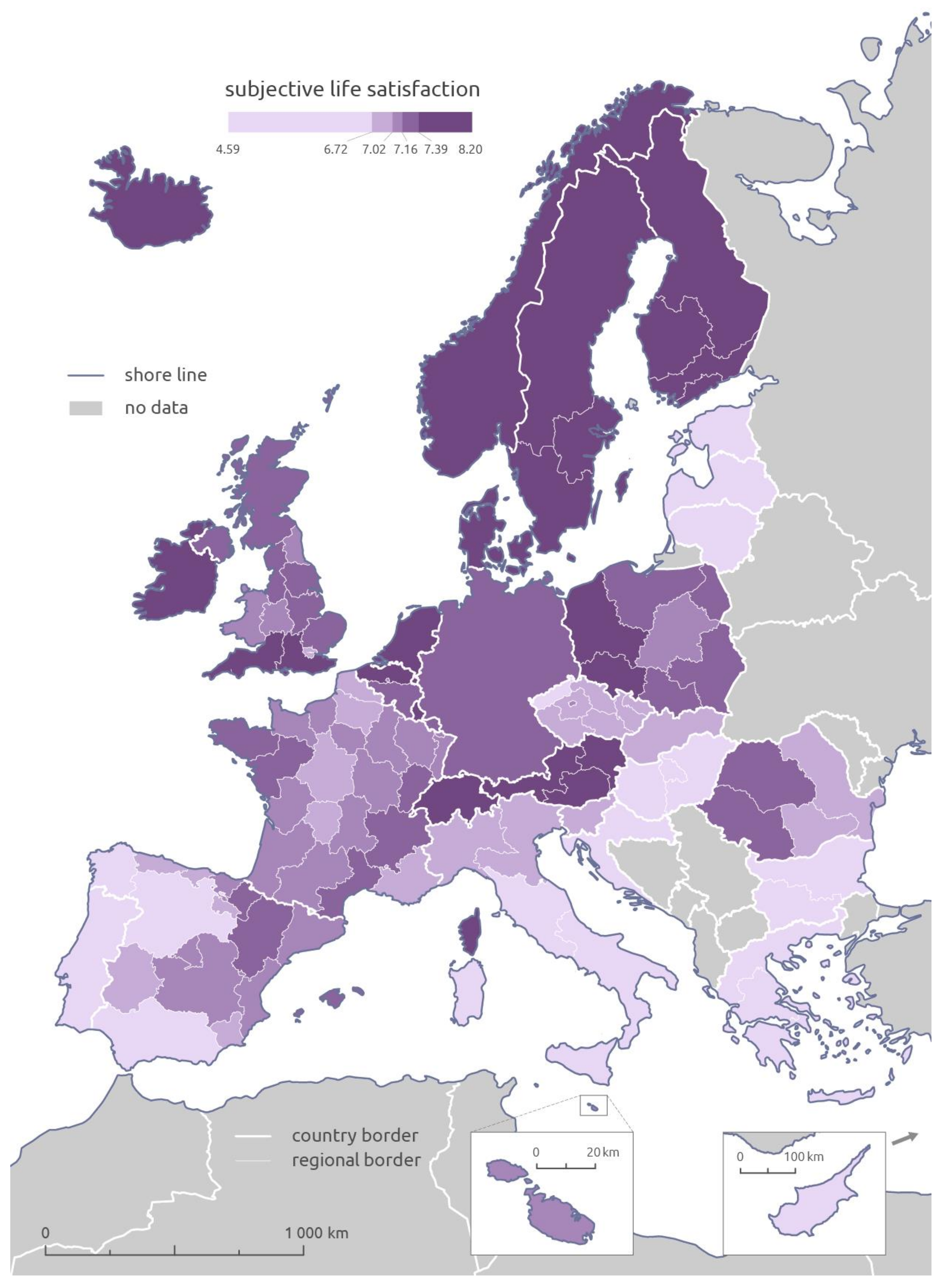
EU-SILC was conducted by Eurostat, and it is the primary data source for a comparative analysis of income and living conditions in the EU. It also provides information that can be used to analyse various aspects of social exclusion [44]. In the future, the EU-SILC dataset is expected to be the main tool in the assessment of quality of life [45]. An ad-hoc module on subjective well-being was implemented in the 2013 EU-SILC, and it included questions about satisfaction with different life domains. For the purpose of this study, the question concerning overall life satisfaction was further elaborated on. Overall life satisfaction shows how a respondent evaluates or appraises his or her life as a whole on the Cantril ladder (0—not at all satisfied to 10—completely satisfied). Figure 1 displays subjective life satisfaction as reported in EU-SILC 2013 datasets and serves as a visual insight into the dataset. The interpretation of the values is incorporated later in the paper in the context of the fuzzy regression analysis.
2.1.2. Objective Data
Defining the set of objective indicators related to subjective life satisfaction is a very challenging task. A vast amount of existing literature presents quality of life assessments with objective data. Many of these studies cannot be used when dealing with the sub-national level of analysis due to the lack of sufficient data (especially the set of quality of life domains and their indicators defined within the European initiative Beyond the GDP [42]). Therefore, a new theoretical framework of quality of life domains was designed. A literature review was vital for the choice of domains. In total, 31 existing studies, which represent practically solved case studies of quality of life evaluation, were examined for the conceptual analysis of the objective set of indicators selection (all studies are listed in Appendix C). This identification faced the issue of using different naming of domains that had to be unified or generalised for a subsequent overview of their occurrence frequency. For example, domains labelled as “education”, “quality of education”, “education and training” and “knowledge” were generalised and merged under the domain named “Education”. The identification of the domains repeatedly included in these studies allowed the definition of the most important ones (here called core domains) that should be included in the analysis.
Domains were subsequently contrasted with the availability of statistical data at the sub-national level. At the sub-national level, the choice of domains must fit in with the availability of the sub-national statistical data as a source of the domains’ indicators. Only Eurostat and the OECD Regional database provide sufficient sub-national statistical data that covers most of Europe. It is not appropriate to compile a dataset by combining data from individual national statistical offices because of the incompatibility and lack of availability of individual data. First, a set of basic indicators (belonging to the core domains) was defined. These are, for example, life expectancy, infant mortality, income, GDP, rates of educated population, etc. Subsequently, all available data were considered in the data sources (only with a focus on a regional level), and other suitable indicators were selected. The criteria for the selection of specific indicators were (a) the inclusion of the indicator in one of the studies from a systematic review and (b) the authors’ subjective assessment of the suitability of indicators. This approach is partially data-driven, but at the moment, it is the only way of compiling a dataset sufficient for quality of life evaluation at the sub-national level.
Since this article is part of a more extensive study focused on assessing quality of life at the sub-national level, the data available at NUTS 2 were initially sought. However, to combine NUTS 2 units with EU-SILC results, the details from each country have been adjusted to reflect the availability of the satisfaction information contained in EU-SILC (see the spatial classification in every country in Figure 1).
The final dataset consists of five core domains and 22 corresponding indicators. Table 1 summarises the data used (for a detailed description of the indicators, see Appendix A). The time period corresponds to the EU-SILC survey, i.e., the year 2013.
2.2. Data analysis
A simple correlation can be used to monitor the relationships between subjective life satisfaction and objective quality of life indicators, and this will reveal the underlying relationships within the presented data. Since subjective satisfaction information has been expressed as a cardinal variable, multiple linear regression can be used for modelling the relationships between subjective satisfaction and a set of objective quality of life indicators. The multiple linear regression analysis is able to assess the significance of the predictor variables in explaining the variability of the dependent variable and to evaluate the quality of the computed model. As mentioned in the introductory chapter, due to the vagueness of life satisfaction, it is more reasonable to use the fuzzy modification of multiple linear regression, which is able to capture the uncertainty related to this type of dependent variable. Due to the use of multiple linear fuzzy regression, the uncertainty associated with the dependent variable is incorporated in the analysis. At the same time, it allows the use of classical computing methods, which are suitable for the analysis of relationships between a dependent variable and its predictors.
A suitable form of multiple fuzzy regression for the data available is a multiple fuzzy regression analysis for non-fuzzy data with asymmetrical fuzzy coefficients, as was defined by Ishibuchi and Nii [46]. In this particular case, both the predictor values and the predicted value are classic (non-fuzzy) values. The multiple fuzzy regression estimates regression coefficients as fuzzy numbers [47]. From a practical perspective, triangular fuzzy numbers [48] are used. Triangular fuzzy numbers (graphically demonstrated in Figure 2) are the simplest fuzzy numbers, which are defined by three values . Triangular fuzzy numbers also allow for the simplest implementation of fuzzy arithmetic, according to Hanss [49]. A fuzzy number consists of so called -cuts; is a value from interval [0,1]. An -cut is an interval with values that have a membership value of at least [49]. For a triangular fuzzy number, the -cut with value 0 is the extent of the fuzzy number . The -cut with value 1 is an interval .
Multiple fuzzy regression for a set of predictor-dependent variable pairs , where , with fuzzy coefficients is calculated as [46]:
for any given .
The determination of fuzzy coefficient is done in two steps [46]. The is determined using least square regression, to determine the centres of fuzzy coefficients . The lower and upper limits are determined by a linear programming problem:
Minimise
subject to
where is a -cut. The parameter specifies the spread of the fuzzy coefficients. The higher the value, the wider the predictions of the fuzzy coefficients. For the practical estimation of fuzzy coefficients, a value of h slightly higher than 0 was used to construct triangular fuzzy numbers. This value means that the fuzzy regression coefficients should be defined in such a way to just cover the predictors’ values. The implementation of the linear programming problem was done using the GLPK software [50]. With known, the estimate can be calculated using fuzzy arithmetic [49].
For a more detailed analysis of the resulting layers (fuzzy model prediction of life satisfaction and its uncertainty), the geographically weighted correlation proposed by Kalogirou [51] was used. This local variation of the correlation coefficient calculates the weighted local correlation in every location (here region) only from k neighbouring observed locations, where k is defined by the user as a percentage of all observations, and weights are based on the Euclidean distance between the observed location and every neighbouring observation.
3. Results
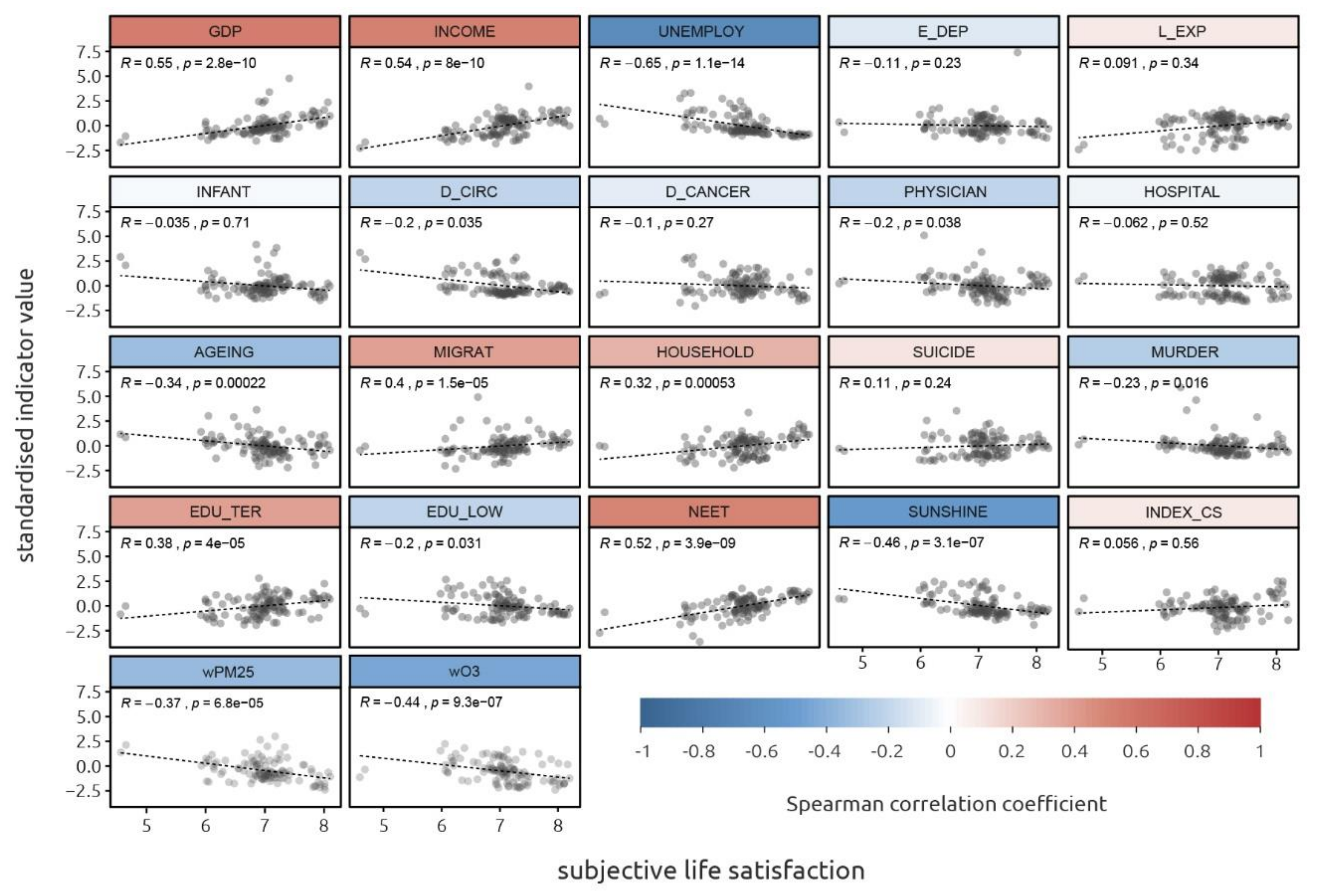
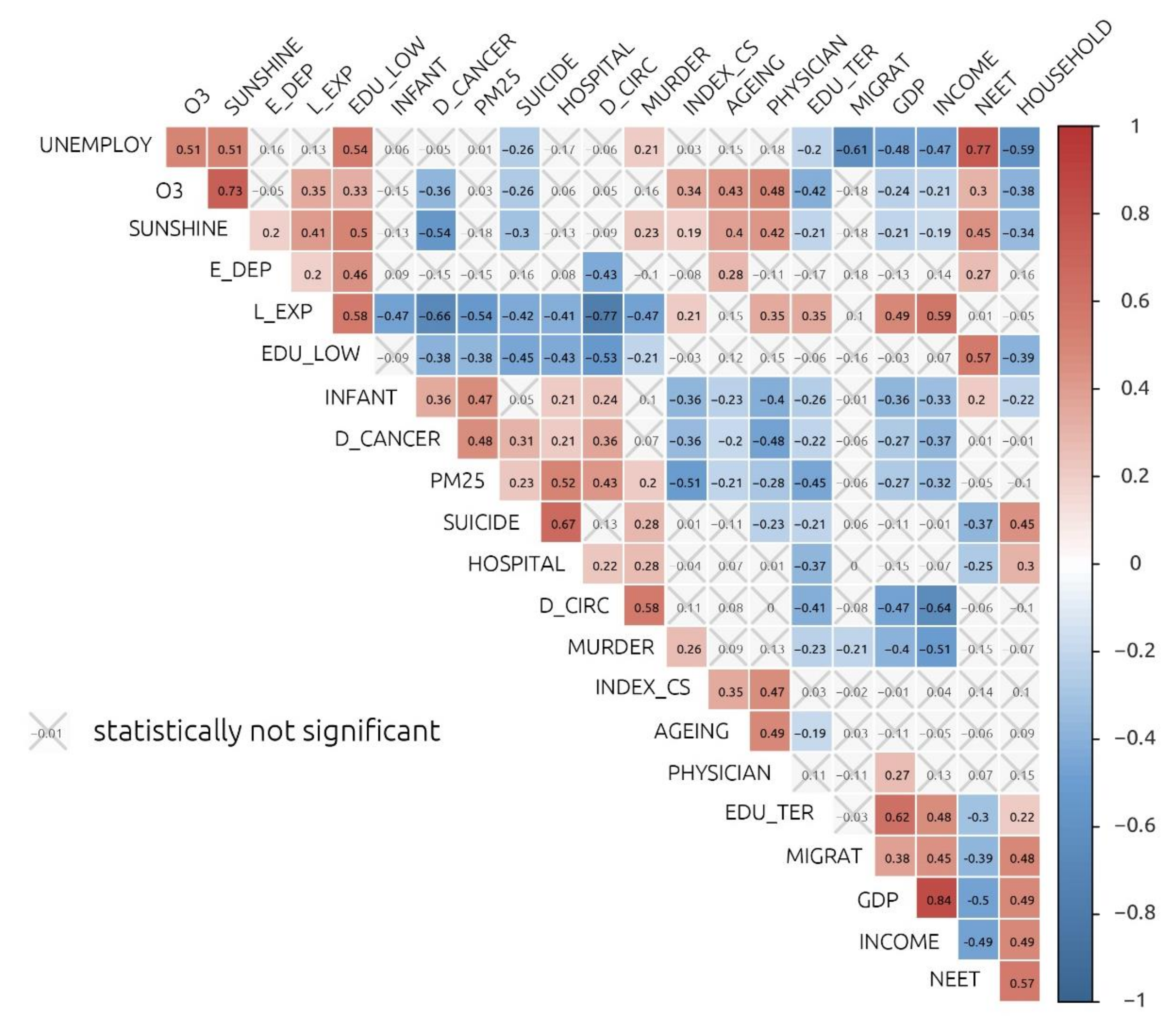
First, the correlation between life satisfaction and the selected objective indicators was calculated. Since the Shapiro–Wilk test did not prove normality, Spearman’s correlation of subjective satisfaction with each independent quality of life indicator from the input dataset was calculated. This initial analysis revealed linear relationships between some of the indicators and subjective life satisfaction (according to De Vaus [52], a correlation coefficient higher than 0.5 can be labelled as significant): UNEMPLOY (−0.65), GDP (0.55), INCOME (0.54), NEET (0.52); medium correlation (correlation coefficient in the range 0.3–0.49) was observed between life satisfaction and the O3 (−0.48), SUNSHINE (−0.46), MIGRAT (0.4), EDU_TER (0.38) and AGEING (−0.34). All the correlations between life satisfaction and the selected quality of life indicators are presented in Figure 3. At the same time, the correlations between all the predictors were calculated. The output correlation matrix is presented in Appendix B.
The next step was to perform a multiple fuzzy regression analysis in order to capture the relationships between life satisfaction and the set of quality of life indicators. At the beginning of the multiple fuzzy regression modelling, the optimal linear model must be identified, which is later calculated as a multiple fuzzy regression model. First, a complex model containing all the input indicators was designed and tested (MODEL1). Intercorrelations among the independent variables can cause statistical inferences (presumptions) based on the data to be unreliable. Therefore, the data were tested for the presence of multicollinearity. For individual predictors, multicollinearity was evaluated using the variance inflation factor (VIF). VIF scores higher than five, indicating significant multicollinearity [53], were reported for several predictors—the VIF values in each model are shown in Table 2:
Since there are significant outliers in the INCOME indicator, it has been transformed in form 1/INCOME. Predictors with a VIF higher than five have been removed from the model, except for INCOME and EDU_TER. Since these indicators are considered very significant on a theoretical basis for quality of life, they have not been excluded from the model. After the removal of high-VIF indicators, MODEL2 was designed, where all of the indicators fulfil the VIF condition. The resulting model, MODEL2, was processed as a multiple fuzzy regression model and is described in Table 3:
where aL is the minimum of that triangular fuzzy number, aC is its centre, aU is the maximum triangular fuzzy number, aC − aL is the difference between the centre and the minimum of the fuzzy number, and aU − aC is the difference between the maximum and centre of the fuzzy number. The intercept (constant) is the expected mean value of the dependent variable, when all predictors equal zero. Seven out of the fourteen predictors were accepted at the significance level of 0.05; the PHYSICIAN predictor was accepted at the level of 0.1.

Table 3.
Fuzzy coefficients of the regression model. Acceptance of the predictor at the significance levels of 0.05 (**) and 0.1 (*).
Table 3.
Fuzzy coefficients of the regression model. Acceptance of the predictor at the significance levels of 0.05 (**) and 0.1 (*).
| Indicator | aL | aC | aU | aC − aL | aU − aC |
|---|---|---|---|---|---|
| intercept | 9.731 | 9.731 | 9.731 | 0 | 0 |
| INCOME ** | −17,766 | −17,766 | −17,766 | 0 | 0 |
| E_DEP | −0.0023 | −0.0023 | −0.0023 | 0 | 0 |
| INFANT ** | −0.0497 | 0.0708 | 0.0708 | 0.1206 | 0 |
| D_CANCER | 0.0001 | 0.0001 | 0.0022 | 0 | 0.0020 |
| PHYSICIAN * | −0.1392 | −0.0895 | −0.0895 | 0.0497 | 0 |
| HOSPITAL ** | −0.0069 | −0.0069 | −0.0069 | 0 | 0 |
| AGEING ** | −0.0055 | -0.0055 | −0.0055 | 0 | 0 |
| MIGRAT | −0.0058 | −0.0058 | −0.0058 | 0 | 0 |
| HOUSEHOLD | 0.0104 | 0.0104 | 0.0104 | 0 | 0 |
| SUICIDE | 0.0007 | 0.0007 | 0.0014 | 0 | 0.0135 |
| MURDER | −0.2509 | 0.0443 | 0.0443 | 0.295 | 0 |
| EDU_TER ** | −0.0146 | −0.0146 | −0.0146 | 0 | 0 |
| NEET ** | −0.0427 | −0.0427 | −0.0423 | 0 | 0.0004 |
| INDEX_CS ** | 0.0923 | 0.0923 | 0.0923 | 0 | 0 |
Nine of the coefficients are classic (non-fuzzy) numbers. These numbers contain no uncertainty at all. The other six variables (INFANT, D_CANCER, PHYSICIAN, SUICIDE, MURDER and NEET) contain at least some uncertainty. The shape of the individual fuzzy values is determined by the linear programming method, which means that it may be possible to find more than one feasible solution (set of fuzzy coefficients). However, all the solutions would provide very similar outcomes, as they have to fulfil the same constraints regarding the data.
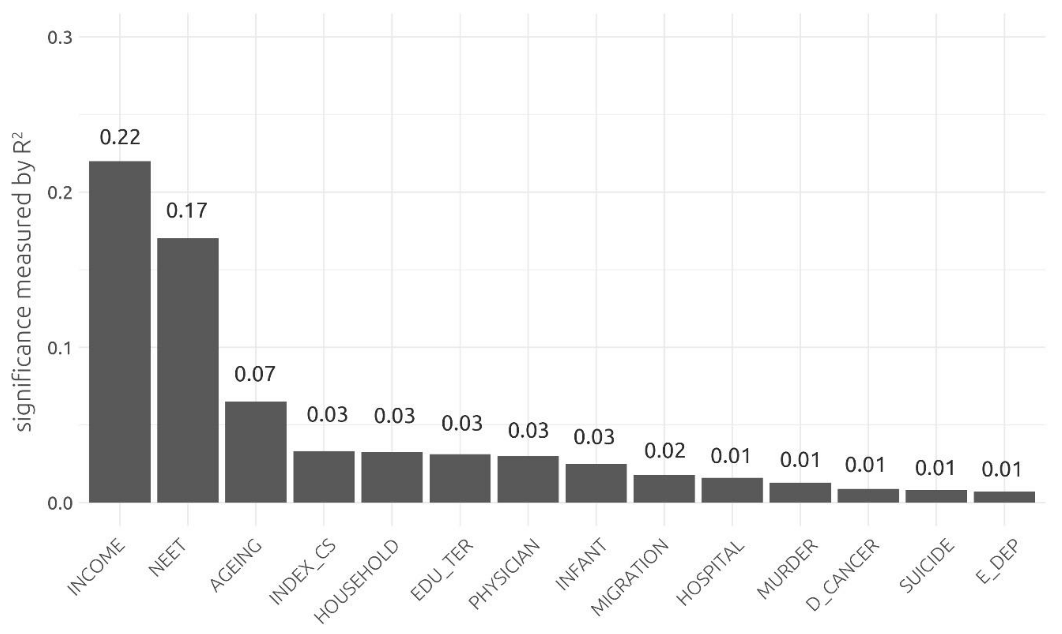
The adjusted R2 value of 0.631 indicates that 63.1% of the variance of subjective life satisfaction can be explained by the selected indicators. The significance of the individual indicators in this model was finally evaluated by the proportion of explained variance (R package dominanceanalysis). According to Azen and Budescu [54], one predictor is more important than another if it contributes more to the prediction than the other at a given level of analysis. The function returned the following significance values for variables measured by R2 (Figure 4). The dominance of the INCOME and NEET predictors is clearly visible.
When the relationship between subjective satisfaction and its predictors is examined, it is also appropriate to interpret and explain the calculated coefficients rather than to only quantify them. Since the fuller model was created, a brief interpretation of only the significant predictors is introduced. Because each of the objective predictors has a different meaning in the context of quality of life, their coefficients in the model were divided into three groups for better interpretation:
- Easy to interpret (INCOME, INDEX_CS, NEET): the relationship of these indicators with life satisfaction is not surprising and can be easily explained. The INCOME indicator (the negative coefficient value caused by the transformation of the input data) proved to be the most significant. It can be agreed that with a better financial situation of the household, the satisfaction of the household members increases. Based on the model, hypothetically, life satisfaction measured with the Cantril Ladder would increase by one point if the household income was increased by approximately 17,800 EUR PPS. Similarly, in the case of INDEX_CS, the quality of the landscape can also be easily perceived and valued. The results suggest that respondents perceive the quality of landscape expressed by the INDEX_CS indicator in a similar way and mostly positively. To implicitly express how a change in the quality of landscape influences subjective satisfaction is not that straightforward, since the quality of the landscape is a complex unitless index. Finally, the NEET indicator, as a measure of the labour market (eventually a measure of the transfer of education to the labour market), can be also perceived in life satisfaction. The concerned group of young people can be affected by growing up under the unfavourable conditions, which might lead to long-term life dissatisfaction. Moreover, this indicator is correlated with overall long-term unemployment (correlation coefficient, 0.77), which leads to material insecurity and has a negative impact in the context of life satisfaction.
- Difficult to interpret (AGEING): the signum of the coefficients of this indicator is the same as the expected meaning in the context of quality of life, but its perception for life satisfaction can be biased. In this case, people living in an old society may perceive this fact negatively, as the ageing of the population can cause social and economic dependencies but also disagreements on a personal level (intergenerational incomprehension).
- “Contra-indicators” (EDU_TER, HOSPITAL, PHYSICIAN, INFANT): this group was expected to increase subjective life satisfaction with higher indicative values, since higher levels of these measures are considered positive quality of life indicators. However, regression coefficients were negative against the assumptions of expected meaning in the context of quality of life. These indicators might have some hidden or indirect relationships with life satisfaction, which are not straightforward to explain.
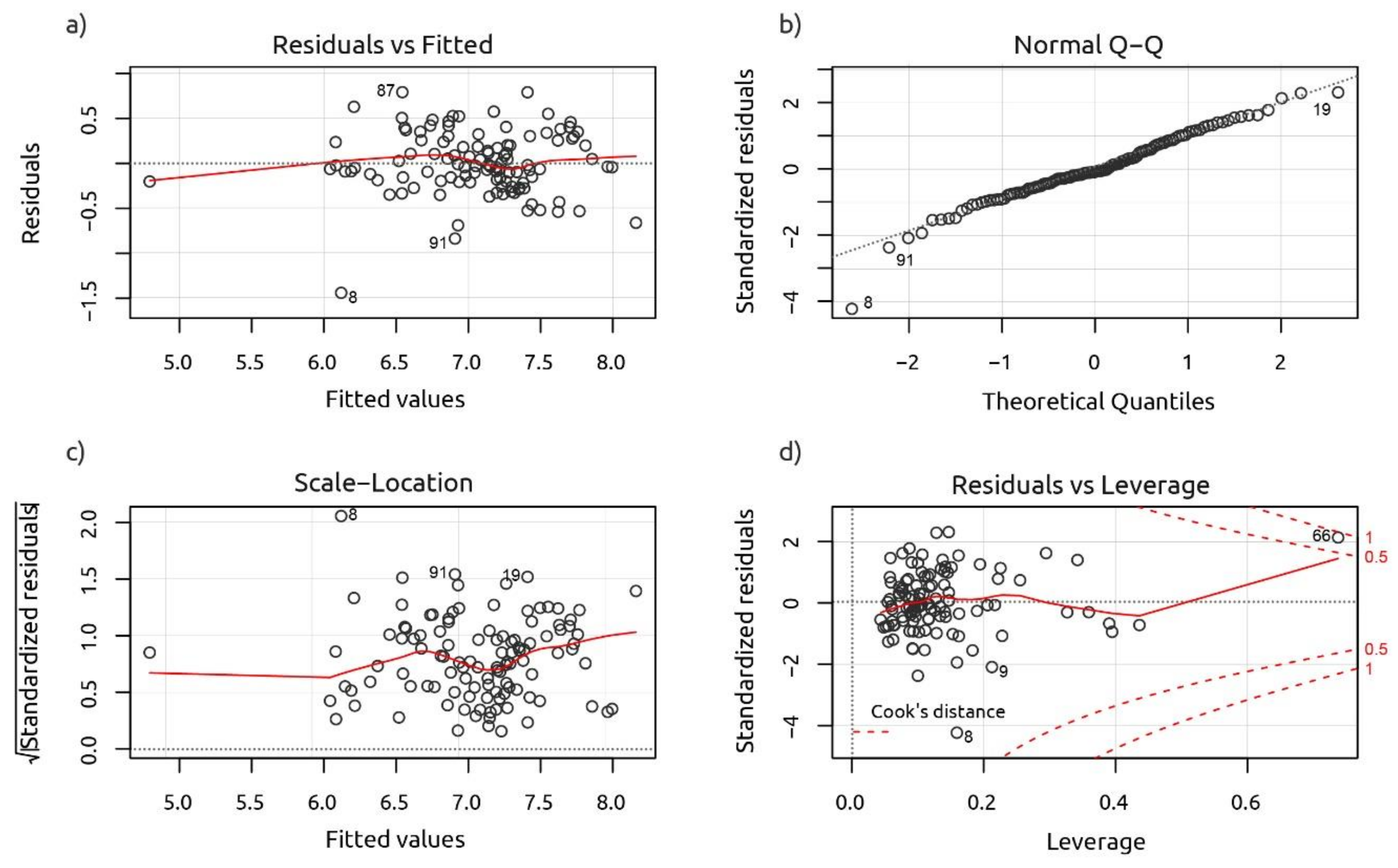
The model was diagnosed to verify the regression modelling assumptions and to evaluate the quality of the obtained model, examining linearity, homoscedasticity, multivariate normality and the influence of outliers. The linearity of the data can be evaluated via the basic graph showing fitted data versus residuals (Figure 5a). There is some distortion in the linear relationship, but no clear pattern is obvious. For the testing of homoscedasticity, the Breusch–Pagan test was used. The test output p-value of 0.24 did not allow the rejection of the null hypothesis that the residuals have a constant variance, so heteroscedasticity was not proven. A visual inspection of homoscedasticity can be done in Figure 5c. The QQ plot of the distribution of the residuals presented in Figure 5b indicates some violation of normality by several records; this assumption has been verified by the Shapiro–Wilk test. The p-value of 0.018 rejects the hypothesis of normal residue distribution. Finally, the presence of outliers was explored; outliers may affect the quality of the model by increasing the residual standard error (RSE) value. Using Cook’s distance, combining leverage and residual size, none of the records were marked as influential outliers (Figure 5d).
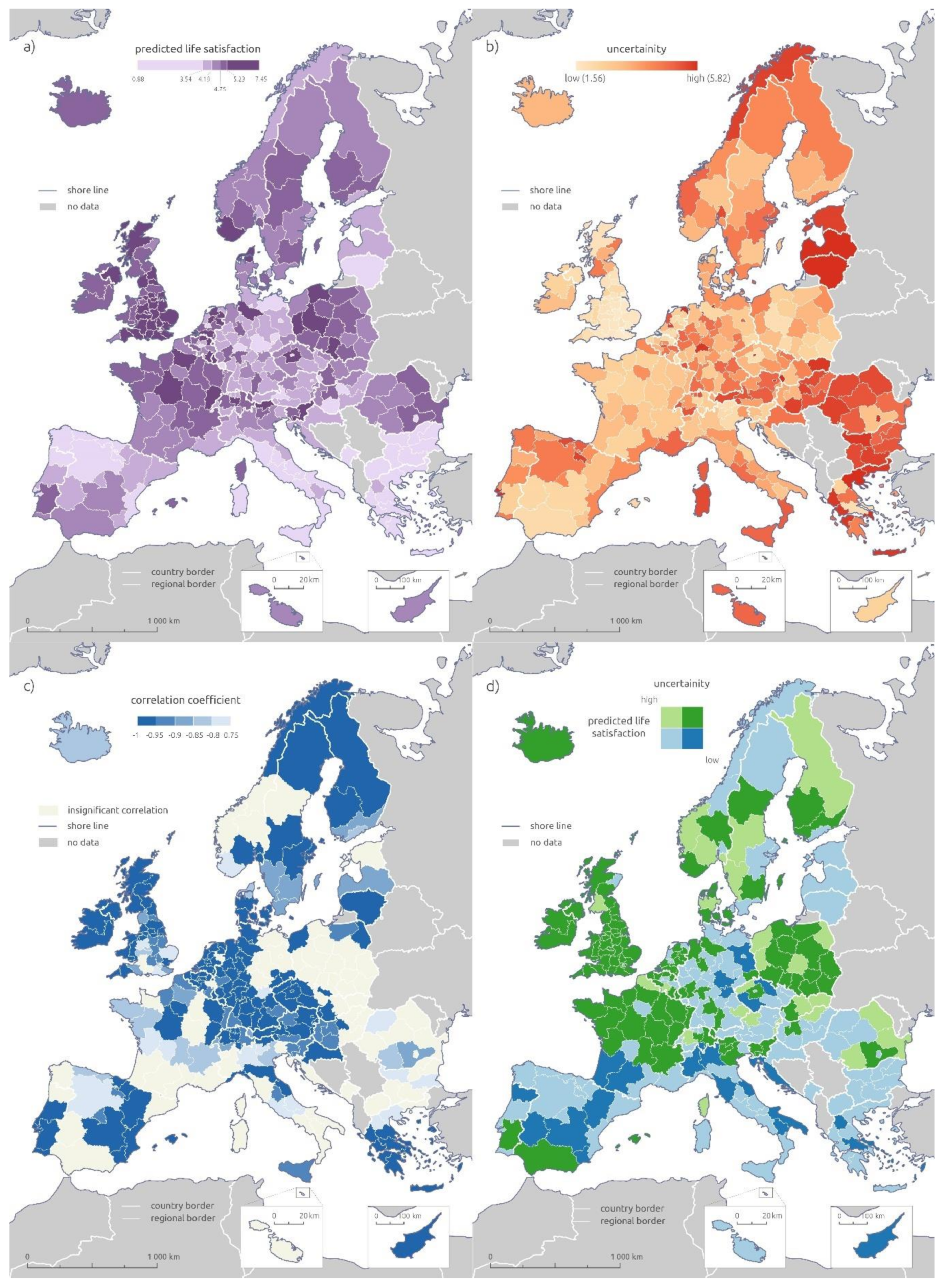
Finally, the multiple fuzzy regression model allows the prediction of life satisfaction with respect to the uncertainty of the relationship between life satisfaction and its predictors. This type of outcome is beneficial for users; the prediction in the form of fuzzy numbers acknowledges the ambiguity of the result. The approach steers away from stating the prediction precisely, which may be undesirable under the conditions of uncertainty. The prediction of life satisfaction was applied to the more detailed spatial data, which cover the majority of Europe at the NUTS 2 level. Although both datasets differ in their spatial resolutions and are therefore difficult to compare, the spatial distributions of predicted values (Figure 6a) of life satisfaction differ significantly from the original input data (Figure 1). The most obvious differences are in regions of Austria and Switzerland, where predicted values are distinctly lower than the original ones. Other examples of differences between predicted and original values are in regions of Romania, France or the United Kingdom. On the other hand, in Belgium and Netherlands, both original and predicted values are high. The prediction also points to the unsuitability of data at the national level—in the case of Germany, the reported satisfaction is rather high, but at the detailed level of the prediction, significant spatial variability can be observed.
Since fuzzy prediction is supplemented by a measure of uncertainty (Figure 6b), it can be clearly visualised along with predicted satisfaction, whereas changes across the area of interest can be observed jointly. The highest value recorded is 5.2. Unfortunately, the predicted uncertainty cannot be interpreted exactly, as it is the result of linear programming, where the interactions between the relationships of the predictors with the dependent variable occur. The presentation of the uncertainty confirms that classical linear models can suppress the great variability and uncertainty, which are revealed only when using a fuzzy approach.
The negative strong relationship between the predicted value and uncertainty was revealed with the correlation test (Spearman’s correlation coefficient, −0.79). To explore the spatial variability of the correlation, geographically weighted correlation was calculated with the neighbourhood defined as 3% of all the regions (Figure 6c), which corresponds, on average, to eight neighbours for every region. This setting provides an appropriate level of detail revealing the spatial heterogeneity of local correlation. Significant values of geographically weighted correlation vary from perfect correlation (−0.99, concentrated in the Germany, Belgium, the Netherlands, Czechia, Greece and parts of the Scandinavia) to strong correlation (−0.75, in France, in Italy and at the Romanian–Bulgarian border). In many cases, other values of local correlation observed in Poland, Romania, east Germany or southern France were statistically insignificant. These areas are atypical and hard to interpret, with fluctuating spatial trends in the relationships between the predicted value and its uncertainty. Since the local measure of correlation does not give any information as to whether the prediction value is high, and uncertainty low (in negatively correlated areas), and vice versa, the result was complemented with simple typology of the regions. All the regions were classified into types according to the predicted value and its uncertainty; the threshold was set by the median. The resulting types were as follows: HH—high predicted satisfaction with high uncertainty, LL—low predicted satisfaction with low uncertainty, HL—high predicted satisfaction with low uncertainty and LH—low predicted satisfaction with high uncertainty. The spatial distribution of the types is shown in Figure 6d. The visualisation of the typology delimits the potentially satisfied areas in Europe, mainly in the north-western part of the continent, the British Isles, Scandinavia and Poland. By contrast, the low prediction of satisfaction is located in a belt stretching from the Iberian Peninsula through the regions of southern Europe and subsequently extending to part of Eastern Europe as well as to Austria and Germany.
4. Discussion
Many studies dealing with the relationship between subjective satisfaction and a set of indicators were introduced. As far as the authors understand, there is no other study at the regional level that examines the links between subjective life satisfaction and the set of objective indicators, covers an extensive part of Europe, and carries out the analysis with the use of fuzzy theory principles.
A crucial part of the presented research was the selection of suitable independent indicators. Since this paper primarily represents an empirical study, the main objective was not to discuss the suitability of the objective indicators monitored, but rather, the ways they are processed. The authors have compiled a sufficient input indicator dataset (based on the literature review) that covers the most important aspects of quality of life, taking into account the critical issue of the lack of availability of detailed sub-national statistical data across Europe.
All the discussed data were entered into the regression modelling process, where some of the objective indicators were removed due to high multicollinearity. Although some sources state that a VIF value of ten is also acceptable [53], the value of 5 was used in order to reduce multicollinearity as much as possible. The adopted model consists of 14 predictors; eight of them are statistically significant at the level of 0.05 or 0.1. There is an alternative solution in the form of stepwise regression, which can identify the most suitable sub-model with the most significant predictors. Since stepwise regression is often criticised for its sensitivity to multicollinearity or data distribution, it was only briefly tested and compared to the full model. A match was found between the significant predictors of the full model and the stepwise model—INCOME, NEET, AGEING, EDU_TER, INDEX_CS, PHYSICIAN and HOSPITAL. Therefore, these indicators may be labelled as “core indicators”, which are important in both approaches. Since the purpose of the regression modelling is to describe life satisfaction with a small number of indicators, consequent interpretation is more straightforward with this reduced core selection. The relationships of other predictors with life satisfaction can be seen in Table 3.
The uncertainty of the predicted values from fuzzy regression might change significantly with the introduction of a new predictor. The reason is that the new predictor may significantly change the linear programming problem used to estimate the fuzzy coefficients of the fuzzy regression. For the same reason, each new predictor can also change the scatter of the uncertainty through the model. Despite these issues, the fuzzy regression models provide valuable outcomes in the form of predictions with uncertainty evaluation, given the data that were used to estimate the linear regression model.
The importance of fuzzy predictions is the most prominent if the outcomes should be used to support planning and decision making. The predicted values in the form of fuzzy numbers naturally capture the uncertainty that is inherently present in any prediction model. This promotes better decision making, as the decision maker obtains a set of possible predictions instead of just a crisp value, which may provide a false impression that the model is accurate and precise. The same issue is applicable to other prediction models [55]. The uncertain predictions can be utilised in a framework of soft computing methods to support decision making with more information and provide significantly richer results, as shown in [56].
The quality of the model, represented by R2 with a value of 0.631, is questionable but may be sufficient in the context of the topic of subjective satisfaction. According to Lucas and Donnellan [57], approximately one third of the overall variance in subjective satisfaction is influenced by random changes in people’s perceptions and states of mind; the remaining two thirds can be explained by external environmental conditions. Since Lucas and Donnellan worked with the determinants of temporal stability (mainly genetics) and variability (mostly external conditions and measurement error) at the level of individuals, their findings are hard to compare with the results of this study. However, this reference can be considered to provide at least roughly approximate information for the evaluation of model quality.
In the model diagnostics, some general assumptions of regression modelling were violated (linearity of relationships and residual normality). Although none of the records were identified as outliers by the model, a more in-depth analysis of the diagnostics revealed a strong influence in input data, specifically (geographically) in the Northern and Eastern Bulgaria regions. An examination of the input indicators in this region revealed that the lowest value was reached in the INCOME indicator, and in the dependent variable of subjective satisfaction, the third-highest value was in the NEET indicator. In the other monitored indicators, the region behaves in an average way. This combination probably contributed to the negative effect on model quality. The problem was partially solved by the transformation of the INCOME indicator.
Previously, the set of resulting indicators labelled as statistically relevant to subjective satisfaction was not presumed. Therefore, these “unexpected” indicators were subject to further description. Three of the indicators were easy to interpret, and some were contradictory to the expected assumptions. Many input indicators were not actually reflected in the model, although their relationship with subjective satisfaction could be expected—suicide rates, for example, were insignificant. In addition, only infant mortality was proved as significant in relation to life satisfaction with Health domain indicators. Since its interpretation is not clear, this indicator was classified into the “contra-indicators” category. Health indicators such as life expectancy and mortality rates are indicators that rather describe a state of society that is not perceived on a personal level. Concerning the relationships mentioned in other studies, only the positive influence of material welfare mentioned by Dolan et al. and Boarinii et al [25,27] and the negative relationship with age [27] represented here by the ageing index can be confirmed. Contrary to expectations, the relationship with the duration of sunshine as observed by Schwarz and Clore or Kämpfer and Mutz [31,58] has not been proven in our research, since the indicator was removed due to its multicollinearity. It might be proxied by another predictor in the model, but the linkage has not been revealed. However, the findings of our study do not need to be questioned, as studies are very difficult to compare anyway (in terms of the numbers of respondents, representative samples, and spatial and temporal resolution). The results revealed in our paper show that a number of indicators describe the quality of the environment or the quality of the state of society rather than measure it, which is reflected on a personal level. More “personally” oriented indicators such as self-reported health, job satisfaction, intensity of social activities and similar would be more suitable for regression analysis, but this type of indicator is, unfortunately, not available at sufficient spatial resolutions (at the NUTS 2 level).
In general, investigations of relationships between subjective life satisfaction and a set of related indicators can be helpful for any policy or process aiming at the improvement of living standards or quality of life. Such an analysis may reveal whether the monitoring of selected indicators is genuinely relevant to the policy. In the long-term monitoring of societal development, the actual impact of the specific policy interventions and their perception by society (or individuals) can be observed. For researchers dealing with the topic of quality of life or life satisfaction, a similar approach provides useful insight into the nature of the phenomenon under investigation, which can be further used, e.g., in the form of a more specific selection of data for the modelling of real-world tasks. A key question remains as to whether outcomes from this type of analysis are reliable and robust enough to be considered as relevant for policy-making processes.
In this particular case, it can be inferred that policies should primarily target the material welfare of the population to improve quality of life. This may not be represented purely by household income but may have more general objectives such as reducing the risk of poverty, material deprivation or social exclusion. These goals are also key policy components of the Europe 2020 strategy.
5. Conclusions
It cannot be denied that the subjective approach to quality of life assessment is an important part of the evaluation methodology. The subjective survey-obtained data may be relevant as a reference source for the validation of objective results. The exploration of the relationships between objective indicators and data describing perceived quality of life can be helpful when selecting input data for the quality of life index design.
Three sub-tasks were carried out to answer the research questions on how objective measures relate to subjective life satisfaction at the sub-national level in Europe. A dataset of 22 objective indicators, which cover the most important domains of quality of life according to world literature, was compiled at the NUTS 2 level. The availability of reliable subjective sub-national data is significantly less than that of the objective data; the finest quality subjective dataset (EU-SILC) only has spatial detail that is used in our study (Figure 1), which is worse than NUTS 2 for an objective dataset on quality of life indicators. Keeping in mind the ambiguity of subjective data, fuzzy theory was applied to the regression models. The relationship between the subjective and objective data was analysed with fuzzy linear regression. Fuzzy regression can handle the uncertainty of regression coefficients as well as the uncertainty of potentially predicted values. When supplemented with spatial visualisation, spatial variability and its patterns, which are very distinct in this case, can be observed. The results from the last research task show only seven indicators with a statistically proven relationship with subjective satisfaction. Moreover, the relationship between five of the seven indicators was difficult to interpret clearly.
The results confirm the findings of the literature review that the suitability of the indicator for modelling subjective satisfaction is very variable, and it is not possible to issue generally valid statements in this respect. Although a number of studies have tested the robustness of the information obtained from individual surveys, the results are always influenced by the state of the respondents, by the sample spatial resolution, and by the time at which the survey was conducted. In our research, we proved that the inherent data uncertainty could be processed by the fuzzy linear regression model. In fact, we were able to capture and explore the relationships between the subjective perception of life satisfaction and the objective measures that are usually used to research quality of life. Our research represents a quantitative contribution to the existing debates on life satisfaction and attempts novel ways of tackling this complex issue. In the future, it would be interesting to test the consistency of the results on other available subjective data at the regional level (Eurobarometer, Eurofound, or OECD Regional Well-Being) and to compare the results obtained by different methods, such as the regression model vs. the machine learning approach, and such as regression trees.
Author Contributions
Conceptualization, Karel Macků; Methodology, Karel Macků, Jan Caha, Vít Pászto, Pavel Tuček; Data Curation, Karel Macků; Writing-Original Draft Preparation, Karel Macků; Writing-Review & Editing, Karel Macků; Vít Pászto; Visualization, Karel Macků. All authors have read and agreed to the published version of the manuscript.
Funding
This paper was created within the project “Innovation and application of geoinformatic methods for solving spatial challenges in the real world.” (IGA_PrF_2020_027) with the support of the Internal Grant Agency of Palacky University Olomouc, by the project of Ministry of Education, Youth and Sports of the Czech Republic (project number LTI17014) and by the European Union, Erasmus+ programme, grant number 2019-1-CZ01-KA203-061374.
Acknowledgments
This study is based on data from Eurostat, EU-SILC 2013.
Conflicts of Interest
The authors declare no conflict of interest.
Appendix A
Table A1.
List of objective indicators with their descriptions.
| Indicator | Unit | Indicator Description |
|---|---|---|
| GDP per capita | euro PPS per capita | Gross domestic product. |
| Net disposable household income per capita | euro PPS per capita | The total income of a household, after tax and other deductions, that is available for spending or saving, divided by the number of household members converted into equalized adults; household members are equalized or made equivalent by weighting each according to their age. |
| Long-term unemployment | % | Expresses the number of long-term unemployed (12 months and more) aged 15–74 as a percentage of the active population of the same age. |
| Economic dependency index | ratio | The ratio of population aged 0–15 and older than 65 years to the size of the economically active population. |
| Life expectancy at birth | year | The mean number of years that a person can expect to live at birth if subjected to current mortality conditions throughout the rest of their life. |
| Infant mortality rate | ‰ | The infant mortality rate is defined as the number of deaths of children under one year of age during the year to the number of live births in that year. The value is expressed per 1000 live births. |
| Death rate—diseases of the circulatory system | ratio | Standardised death rate (weighted average of age-specific mortality rates) caused by diseases of the circulatory system according to the International Statistical Classification of Diseases and Related Health Problems (categories I00–I99). Expressed as a rate per 100,000 inhabitants. |
| Death rate—diseases of the circulatory system | ratio | Standardised death rate (weighted average of age-specific mortality rates) caused by malignant neoplasms according to the International Statistical Classification of Diseases and Related Health Problems (categories C00–C97). Expressed as a rate per 100,000 inhabitants. |
| Physician rate | ratio | The number of physicians per 10,000 inhabitants. |
| Hospital capacity rate | ratio | The number of hospital beds per 10,000 inhabitants. |
| Ageing index | ratio | The ratio of the population older than 65 years to the population aged 0–15. |
| Migration | ratio | Crude rate of net migration (including statistical adjustment during the year to the average population in that year). Three-year average was applied; data expressed as a rate per 10,000 inhabitants. |
| Household size | % | Ratio of one person households to the total number of households. |
| Suicide rate | ratio | Derived from the death rate caused by an intentional self-harm according to the International Statistical Classification of Diseases and Related Health Problems (categories X60–X84). Expressed as a rate per 100,000 inhabitants. |
| Criminality (murder rate) | ratio | Derived from the death rate caused by an assault according to the International Statistical Classification of Diseases and Related Health Problems (categories X85–Y09). Expressed as a rate per 100,000 inhabitants. |
| Ratio of tertiary educated | % | Defined as the percentage of the population aged 25–64 who successfully completed tertiary studies. This education level refers to ISCED (International Standard Classification of Education) 2011 level 5–8. |
| Ratio of low educated | % | Defined as the percentage of the population aged 25–64 who successfully completed less than primary or primary and lower secondary education. This education level refers to ISCED (International Standard Classification of Education) 2011 level 0–2. |
| NEET | % | Young people aged between 15 and 24, Neither in Employment nor Education or Training. |
| Sunshine duration | hour | Annual sum of sunshine duration. |
| Quality of landscape | index | Cultural function of the landscape based on the study by Burkhard et al. [59]. Index calculated from the Corine Land Cover 2012 as the average area-weighted score. |
| Ozone concentration (SOMO35) | μg·m−3·day | The annual average of the sum of the amounts by which maximum daily 8-h concentrations (in μg·m−3) exceed 70 μg·m−3 on each day in a calendar year. |
| Air pollution (PM2.5 particles) | μg·m−3 | The annual mean PM2.5 concentrations based on interpolation of observed values in control stations. |
Appendix B
Figure A1.
Correlation matrix for all input objective indicators.

Appendix C
Table A2.
A list of studies from the literature review and their domains of quality of life.
| Author | Domains Used |
|---|---|
| Greyling and Tregenna (2017) [21] | housing, social relationships, economic dimension, health, governance, civic engagement, safety, life satisfaction, environmental satisfaction |
| Dasgupta and Weale (1992) [60] | income, life expectancy, infant mortality, adult literacy, political rights, civil rights |
| González, Cárcaba and Ventura (2011) [61] | health, education, personal activities, housing, political voice, social connections, environmental conditions, personal/economic insecurity |
| Martín and Mendoza (2013) [20] | health, education, personal activities, political voice and government, social connections, environmental conditions, personal/economic insecurity |
| Rao et al. (2012) [62] | environmental conditions, material welfare, population |
| Morais and Camanho (2011) [5] | demography, social aspects, economic aspects, training and education, environment, transport and travel, information society, culture and recreation |
| Felce and Perry (1995) [63] | physical wellbeing, material wellbeing, social wellbeing, development and activities, emotional wellbeing |
| Murgaš and Klobučník (2016) [64] | family, health, education, job, natural environment |
| Lo and Faber (1997) [65] | land cover, NDVI, population density, income, home value, college graduates |
| Li and Weng (2007) [66] | population density, housing density, green vegetation, surface temperature, family income, per capita income, poverty level, college graduates, unemployment, house value, number of rooms |
| Bérenger and Verdier-Chouchane (2007) [17] | standard of health, standard of education, material wellbeing |
| Lagas et al. (2015) [40] | public services, purchasing power and employment, housing, social environment, natural environment, recreation, health, education, governance |
| Baliamoune-Lutz and McGillivray (2006) [67] | health, education, income |
| Hancock (2000) [68] | social aspect, health, economic aspect, environmental aspect |
| Puskorius (2015) [69] | health, employment and occupancy rate, environment, lifetime, income, consumption, consumption, environment, accommodation education, spiritual, moral-ethical and cultural values, gender equality, safety, law, order, corruption |
| Morris (1978) [70] | health, education |
| Hardeman and Dijkstra (2014) [71] | health, knowledge, income |
| Eurostat (2015) [35] | material living conditions, employment, education, health, leisure and social interactions, economic and physical safety, governance and basic rights, natural and living environment, overall life satisfaction |
| Annoni, Weziak-Bialowolska, and Dijkstra (2012) [39] | earnings and income, absolute poverty, relative poverty, objective health, subjective health |
| United Nations Development Programme (1990) [72] | long and healthy life, knowledge, a decent standard of living |
| OECD (2011) [23] | income, job, housing, health, education, environment, safety, civil engagement, accessibility of services, community, life satisfaction |
| UK Deprivation index (2007) | income, employment, education, skills and training, health, crime, barriers to housing and services, access to services, housing, physical environment |
| Smith (1972) [73] | income, wealth and employment, environment, health, social disorganisation, alienation and participation, education |
| Veenhoven (1996) [74] | life expectancy, life satisfaction |
| Diener (1995) [75] | physicians per capita, subjective wellbeing, university attendance, income equality, major environmental treaties, monetary savings rate, income per capita |
| Pena and Somarriba (2008) [37] | employment, accommodation, education, leisure, income, health, social relations, satisfaction |
| Glatzer (2007) [1] | health, wealth, knowledge, freedom & governance, equity |
| Rahman et al. (2005) [22] | social relations, emotional wellbeing, health, job, material wellbeing, community participation, safety, quality of environment |
| Veneri and Murtin (2018) [76] | income, health, job |
| Canadian Wellbeing Index (2011) | community vitality, democratic engagement, education, environment, healthy population, leisure and culture, living standards, time use |
| European Index of Social Progress (2016) | nutrition and basic medical care, shelter, personal safety, access to basic knowledge, access to information and communication technology, environmental quality, personal rights, tolerance and inclusion |
References
- Glatzer, W. Quality of Life in the European Union and the United States of America: Evidence from Comprehensive Indices. Appl. Res. Qual. Life 2007, 1, 169–188. [Google Scholar] [CrossRef]
- Smith, D.M. The Geography of Social Well-Being in the United States: An Introduction to Territorial Social Indicators. Soc. Indic. Res. 1973, 1, 257–259. [Google Scholar]
- Campbell, A.; Converse, P.E.; Rodgers, W.L. The Quality of American Life: Perceptions, Evaluations and Satisfactions; Russell Sage Foundation: New York NY, USA, 1976; ISBN 9780871541949. [Google Scholar]
- Andrews, F.M. Research on the Quality of Life; Survey Research Center—Instiute of Social Research: Ann Arbor, MI, USA, 1986; ISBN 9780879443085. [Google Scholar]
- Morais, P.; Camanho, A.S. Evaluation of performance of European cities with the aim to promote quality of life improvements. Omega 2011, 39, 398–409. [Google Scholar] [CrossRef] [Green Version]
- Liu, B.C. Quality of Life Indicators in U.S. Metropolitan Areas: A Statistical Analysis. In Praeger Special Studies in U.S. Economic, Social, and Political Issues; Praeger: New York NY, USA, 1976. [Google Scholar]
- Emerson, E. Evaluating the impact of deinstitutionalization on the lives of mentally retarded people. Am. J. Ment. Defic. 1985, 90, 277–288. [Google Scholar]
- Meeberg, G.A. Quality of life: A concept analysis. J. Adv. Nurs. 1993, 18, 32–38. [Google Scholar] [CrossRef]
- Cummins, R.A. The Comprehensive Quality of Life Scale—Intellectual/Cognitive Disability; School of Psychology: Melbourne, Australia, 1997; ISBN 07300-27252. [Google Scholar]
- Somarriba, N.; Pena, B. Synthetic indicators of quality of life in Europe. Soc. Indic. Res. 2009, 94, 115–133. [Google Scholar] [CrossRef]
- Andráško, I. Quality of Life: An Introduction to the Concept; Masarykova Univerzita: Brno, Czech Republic, 2013; ISBN 978-80-210-6669-4. [Google Scholar]
- Cantril, H. The Pattern of Human Concerns; Rutgers University Press: New Jersey NJ, USA, 1965. [Google Scholar]
- Diener, E.; Suh, E. Measuring quality of life: Economic, social, and subjective indicators. Soc. Indic. Res. 1997, 40, 189–216. [Google Scholar] [CrossRef]
- Kahneman, D.; Krueger, A.B. Developments in the Measurement of Subjective Well-Being. J. Econ. Perspect. 2006, 20, 3–24. [Google Scholar] [CrossRef] [Green Version]
- Dodge, R.; Daly, A.; Huyton, J.; Sanders, L. The challenge of defining wellbeing. Int. J. Wellbeing 2012, 2, 222–235. [Google Scholar] [CrossRef] [Green Version]
- Cambridge University Press Well-being. Available online: https://dictionary.cambridge.org/dictionary/english/well-being (accessed on 18 June 2019).
- Bérenger, V.; Verdier-Chouchane, A. Multidimensional Measures of Well-Being: Standard of Living and Quality of Life Across Countries. World Dev. 2007, 35, 1259–1276. [Google Scholar] [CrossRef]
- Easterlin, R.A. Does Economic Growth Improve the Human Lot? Some Empirical Evidence. In Nations and Households in Economic Growth; David, P.A., Reder, M.W., Eds.; Elsevier: New York, NY, USA, 1974; Volume 8, pp. 89–125. [Google Scholar]
- Mederly, P.; Novacek, P.; Topercer, J. Sustainable development assessment: Quality and sustainability of life indicators at global, national and regional level. Foresight 2003, 5, 42–49. [Google Scholar] [CrossRef]
- Martín, J.C.; Mendoza, C. A DEA Approach to Measure the Quality-of-Life in the Municipalities of the Canary Islands. Soc. Indic. Res. 2013, 113, 335–353. [Google Scholar] [CrossRef]
- Greyling, T.; Tregenna, F. Construction and Analysis of a Composite Quality of Life Index for a Region of South Africa. Soc. Indic. Res. 2017, 131, 887–930. [Google Scholar] [CrossRef]
- Rahman, T.; Mittelhammer, R.C.; Wandschneider, P. Measuring the Quality of Life across Countries A Sensitivity Analysis of Well-being Indices; World Institute for Development Economic Research: Helsinki, Finland, 2005; Volume 5, ISBN 9291906735. [Google Scholar]
- OECD OECD Well Being Indicators Compendium; OECD Publishinig: Paris, France, 2011.
- Oswald, A.J.; Wu, S. Objective Confirmation of Subjective Measures of Human Well-Being: Evidence from the U.S.A. Science 2010, 327, 576–579. [Google Scholar] [CrossRef] [Green Version]
- Boarinii, R.; Comolai, M.; Smith, C.; Machin, R.; de Keulenaerii, F. What Makes for a Better Life. In The Determinants of Subjective Well-Being in OECD Countries—Evidence from the Gallup World Poll; OECD Publishing: Paris, France, 2012. [Google Scholar]
- Hoskins, P.; May, D. The Determinants of Life Satisfaction. In Proceedings of the International Association for Research in Income and Wealth General Conference, Dresden, Germany, 21–27 May 2016. [Google Scholar]
- Dolan, P.; Peasgood, T.; White, M. Do we really know what makes us happy? A review of the economic literature on the factors associated with subjective well-being. J. Econ. Psychol. 2008, 29, 94–122. [Google Scholar] [CrossRef]
- Clark, A.E.; Oswald, A.J. Satisfaction and comparison income. J. Public Econ. 1996, 61, 359–381. [Google Scholar] [CrossRef] [Green Version]
- Layard, R. Happiness: Lessons from a New Science, 2nd ed.; Allen Lane: London, UK, 2005; ISBN 9780713997699. [Google Scholar]
- Poláčková, J.; Jindrová, A. Measurement of Life Satisfaction across the Czech Republic. Statistika 2011, 48, 35–45. [Google Scholar]
- Kämpfer, S.; Mutz, M. On the Sunny Side of Life: Sunshine Effects on Life Satisfaction. Soc. Indic. Res. 2011, 110, 579–595. [Google Scholar] [CrossRef]
- Haslauer, E.; Delmelle, E.C.; Keul, A.; Blaschke, T.; Prinz, T. Comparing Subjective and Objective Quality of Life Criteria: A Case Study of Green Space and Public Transport in Vienna, Austria. Soc. Indic. Res. 2014, 124, 911–927. [Google Scholar] [CrossRef]
- Zadeh, L.A. Fuzzy sets. Inf. Control 1965, 8, 338–353. [Google Scholar] [CrossRef] [Green Version]
- Tanaka, H.; Satoru, U.; Asai, K. Linear Regression Analysis with Fuzzy Model. IEEE Trans. Syst. Man. Cybern. 1982, 12, 903–907. [Google Scholar]
- Rogge, N.; Van Nijverseel, I. Quality of Life in the European Union: A Multidimensional Analysis. Soc. Indic. Res. 2019, 141, 765–789. [Google Scholar] [CrossRef]
- Ivaldi, E.; Bonatti, G.; Soliani, R. The Construction of a Synthetic Index Comparing Multidimensional Well-Being in the European Union. Soc. Indic. Res. 2016, 125, 397–430. [Google Scholar] [CrossRef]
- Pena, B.; Somarriba, N. Quality of life and subjective welfare in Europe: An econometric analysis. Appl. Econom. Int. Dev. 2008, 8, 55–66. [Google Scholar]
- Eurostat Quality of Life—Facts and Views; Publications Office of the European Union: Luxembourg, 2015; ISBN 978-92-79-43616-1.
- Annoni, P.; Weziak-Bialowolska, D.; Dijkstra, L. Quality of Life at the Sub-National Level: An Operational Example for the EU.; Publications Office of the European Union: Luxembourg, 2012; Volume EUR 25630, ISBN 9789279277436. [Google Scholar]
- Lagas, P.; Kuiper, R.; Van Dongen, F.; Van Rijn, F.; Amsterdam, H. Van Regional quality of living in Europe. J. ERSA 2015, 2, 1–26. [Google Scholar]
- Petrucci, A.; D’Andrea, S.S. Quality of Life in Europe: Objective and Subjective Indicators. In Advances in Quality of Life Research 2001; Zumbo, B.D., Ed.; Springe: Berlin/Heidelberg, Germany, 2002; pp. 55–88. ISBN 978-90-481-6209-3. [Google Scholar]
- European Commission Communication from the Commission to the Council and the European Parliament on the GDP and Beyond: Measuring Progress in a Changing World; European Union: European Commision: Brussels, Belgium, 2009.
- European Commission Commission Staff Working Document: Progress on “GDP and Beyond” Actions; European Union: Brussels, Belgium, 2013; Volume 1.
- Di Meglio, E. Living Conditions in Europe, 2018th ed.; Meglio, E., Di Kaczmarek-Firth, A., Litwinska, A., Rusu, C., Eds.; Publications Office of the European Union: Luxembourg, 2018; ISBN 978-92-79-86498-8. [Google Scholar]
- Sponsorship Group on Measuring Progress, Well-being and Sustainable Development. Final Report adopted by the European Statistical System Committee; European Statistical System: Luxembourg, 2011; Available online: https://ec.europa.eu/eurostat/documents/7330775/7339383/SpG-Final-report-Progress-wellbeing-and-sustainable-deve/428899a4-9b8d-450c-a511-ae7ae35587cb (accessed on 11 May 2020).
- Ishibuchi, H.; Nii, M. Fuzzy regression using asymmetric fuzzy coefficients and fuzzified neural networks. Fuzzy Sets Syst. 2001, 119, 273–290. [Google Scholar] [CrossRef]
- Nahmias, S. Fuzzy variables. Fuzzy Sets Syst. 1978, 1, 97–110. [Google Scholar] [CrossRef]
- Anile, A.M.; Deodato, S.; Privitera, G. Implementing fuzzy arithmetic. Fuzzy Sets Syst. 1995, 72, 239–250. [Google Scholar] [CrossRef]
- Hanss, M. Applied Fuzzy Arithmetic; Springer Heidelberg: Berlin/Heidelberg, Germany, 2005; ISBN 978-3-540-24201-7. [Google Scholar]
- Makhorin, A. GLPK (GNU Linear Programming Kit); Department for Applied Informatics, Moscow Aviation Institute: Moscow, Russia, 2012. [Google Scholar]
- Kalogirou, S. Testing local versions of correlation coefficients. Jahrb. für Reg. 2012, 32, 45–61. [Google Scholar] [CrossRef]
- De Vaus, D. Analyzing Social Science Data; SAGE Publications Ltd: London, UK, 2002; ISBN 978-0761959380. [Google Scholar]
- James, G.; Witten, D.; Hastie, T.; Tibshirani, R. An Introduction to Statistical Learning. In Springer Texts in Statistics; Springer New York: New York, NY, USA, 2014; ISBN 978-1-4614-7137-0. [Google Scholar]
- Azen, R.; Budescu, D.V. The dominance analysis approach for comparing predictors in multiple regression. Psychol. Methods 2003, 8, 129–148. [Google Scholar] [CrossRef]
- Caha, J.; Marek, L.; Dvorský, J. Predicting PM 10 Concentrations Using Fuzzy Kriging. In Hybrid Artificial Intelligent Systems; Springer International Publishing: Berlin/Heidelberg, Germany, 2015; pp. 371–381. ISBN 978-3-319-19643-5. [Google Scholar]
- Caha, J.; Nevtípilová, V.; Dvorský, J. Constraint and Preference Modelling for Spatial Decision Making with Use of Possibility Theory. In Hybrid Artificial Intelligence Systems; Springer International Publishing: Berlin/Heidelberg, Germany, 2014; pp. 145–155. ISBN 978-3-319-07616-4. [Google Scholar]
- Lucas, R.E.; Donnellan, M.B. How stable is happiness? Using the STARTS model to estimate the stability of life satisfaction. J. Res. Pers. 2007, 41, 1091–1098. [Google Scholar] [CrossRef] [PubMed] [Green Version]
- Schwarz, N.; Clore, G.L. Mood, misattribution, and judgments of well-being: Informative and directive functions of affective states. J. Pers. Soc. Psychol. 1983, 45, 513–523. [Google Scholar] [CrossRef]
- Burkhard, B.; Kroll, F.; Müller, F.; Windhorst, W. Landscapes’ capacities to provide ecosystem services—A concept for land-cover based assessments. Landsc. Online 2009, 15, 1–22. [Google Scholar] [CrossRef]
- Dasgupta, P.; Weale, M. On measuring the quality of life. World Dev. 1992, 20, 119–131. [Google Scholar] [CrossRef]
- González, E.; Cárcaba, A.; Ventura, J. Quality of life ranking of spanish municipalities. Rev. Econ. Apl. 2011, 29, 123–148. [Google Scholar]
- Rao, K.R.M.; Kant, Y.; Gahlaut, N.; Roy, P.S. Assessment of Quality of Life in Uttarakhand, India using geospatial techniques. Geocarto Int. 2012, 27, 315–328. [Google Scholar] [CrossRef]
- Felce, D.; Perry, J. Quality of life: Its definition and measurement. Res. Dev. Disabil. 1995, 16, 51–74. [Google Scholar] [CrossRef]
- Murgaš, F.; Klobučník, M. Municipalities and Regions as Good Places to Live: Index of Quality of Life in the Czech Republic. Appl. Res. Qual. Life 2016, 11, 553–570. [Google Scholar] [CrossRef]
- Lo, C.P.; Faber, B.J. Integration of landsat thematic mapper and census data for quality of life assessment. Remote Sens. Environ. 1997, 62, 143–157. [Google Scholar] [CrossRef]
- Li, G.; Weng, Q. Measuring the quality of life in city of Indianapolis by integration of remote sensing and census data. Int. J. Remote Sens. 2007, 28, 249–267. [Google Scholar] [CrossRef]
- Baliamoune-Lutz, M.; McGillivray, M. Fuzzy well-being achievement in Pacific Asia. J. Asia Pacific Econ. 2006, 11, 168–177. [Google Scholar] [CrossRef] [Green Version]
- Hancock, T. Quality of life indicators and the DHC. South-eastern Ontario 2000. [Google Scholar]
- Puskorius, S. The Methodology of Calculation the Quality of Life Index. Int. J. Inf. Educ. Technol. 2015, 5, 156–159. [Google Scholar] [CrossRef] [Green Version]
- Morris, M.D. A physical quality of life index. Urban Ecol. 1978, 3, 225–240. [Google Scholar] [CrossRef]
- Hardeman, S.; Dijkstra, L. The EU Regional Human Development Index; Publication Office of the European Union: Luxembourg, 2014; ISBN 9789279398612. [Google Scholar]
- United Nations Development Programme Human Development Report 1990; Oxford University Press: New York, NY, USA, 1990.
- Smith, D.M. Geography and social indicators. South African Geogr. J. 1972, 54, 43–57. [Google Scholar] [CrossRef]
- Veenhoven, R. Happy life-expectancy. Soc. Indic. Res. 1996, 39, 1–58. [Google Scholar] [CrossRef] [Green Version]
- Diener, E. A Value Based Index for Measuring National Quality of Life. Soc. Indic. Res. 1995, 36, 107–127. [Google Scholar] [CrossRef]
- Veneri, P.; Murtin, F. Where are the highest living standards? Measuring well-being and inclusiveness in OECD regions. Reg. Stud. 2018, 53, 657–666. [Google Scholar] [CrossRef]
Figure 1.
Subjective life satisfaction reported in European Union Statistics on Income and Living Conditions (EU-SILC) 2013.
Figure 1.
Subjective life satisfaction reported in European Union Statistics on Income and Living Conditions (EU-SILC) 2013.

Figure 2.
Triangular fuzzy number.

Figure 3.
Correlation between the standardised values of the objective indicators and subjective life satisfaction.
Figure 3.
Correlation between the standardised values of the objective indicators and subjective life satisfaction.

Figure 4.
The significance of predictors in MODEL3.

Figure 5.
(a) Regression model diagnostic plots: linearity of residuals; (b) deviation of residues from normality; (c) homoskedasticity of residuals; (d) indentification of potential influential outliers
Figure 5.
(a) Regression model diagnostic plots: linearity of residuals; (b) deviation of residues from normality; (c) homoskedasticity of residuals; (d) indentification of potential influential outliers

Figure 6.
(a) Predicted values of life satisfaction at the NUTS 2 level (b) supplemented with the level of the prediction uncertainty, (c) the spatial variability of the relationship between uncertainty and predicted satisfaction as demonstrated by the geographically weighted correlation and (d) the typology based on uncertainty and predicted satisfaction.

Table 1.
Overview of the core quality of life domains and their indicators.
| Domain | Aspect | Unit | Abbreviation |
|---|---|---|---|
| Economic and material welfare | GDP per capita | PPS euro per capita | GDP |
| Net disposable household income per capita | PPS euro per capita | INCOME | |
| Long-term unemployment | % | UNEMPLOY | |
| Economic dependency index | ratio | E_DEP | |
| Health | Life expectancy at birth | year | L_EXP |
| Infant mortality rate | ‰ | INFANT | |
| Death rate—diseases of the circulatory system | rate per 100,000 inhabitants | D_CIRC | |
| Death rate—malignant neoplasms | rate per 100,000 inhabitants | D_CANCER | |
| Social environment | Physician rate | rate per 10,000 inhabitants | PHYSICIAN |
| Hospital capacity rate | rate per 10,000 inhabitants | HOSPITAL | |
| Ageing index | ratio | AGEING | |
| Migration | rate per 10,000 inhabitants | MIGRAT | |
| Household size | % | HOUSEHOLD | |
| Suicide rate | rate per 100,000 inhabitants | SUICIDE | |
| Criminality (murder rate) | rate per 100,000 inhabitants | MURDER | |
| Education | Ratio of tertiary educated | % | EDU_TER |
| Ratio of low educated | % | EDU_LOW | |
| NEET | % | NEET | |
| Natural environment | Sunshine duration | hour | SUNSHINE |
| Quality of landscape | index | INDEX_CS | |
| Air pollution (PM2.5) | μg·m−3 | PM25 | |
| Ozone concentration (SOMO35) | μg·m−3·day | O3 |
Table 2.
Variance inflation factor (VIF) in different models.
| MODEL1 | MODEL2 | |
|---|---|---|
| GDP | 9.25 | x |
| INCOME | 9.73 | 3.76 |
| UNEMPLOY | 6.89 | x |
| E_DEP | 2.56 | 1.53 |
| L_EXP | 36.12 | x |
| INFANT | 3.35 | 1.83 |
| D_CIRC | 27.41 | x |
| D_CANCER | 4.22 | 1.78 |
| PHYSICIAN | 2.91 | 1.81 |
| HOSPITAL | 4.68 | 3.02 |
| AGEING | 2.43 | 1.61 |
| MIGRAT | 2.58 | 2.05 |
| HOUSEHOLD | 3.67 | 2.16 |
| SUICIDE | 3.57 | 3.02 |
| MURDER | 2.95 | 1.80 |
| EDU_TER | 5.44 | 2.64 |
| EDU_LOW | 7.75 | x |
| NEET | 4.86 | 2.26 |
| SUNSHINE | 7.51 | x |
| INDEX_CS | 3.37 | 1.57 |
| PM25 | 5.02 | x |
| O3 | 7.51 | x |
© 2020 by the authors. Licensee MDPI, Basel, Switzerland. This article is an open access article distributed under the terms and conditions of the Creative Commons Attribution (CC BY) license (http://creativecommons.org/licenses/by/4.0/).
Share and Cite
MDPI and ACS Style
Macků, K.; Caha, J.; Pászto, V.; Tuček, P. Subjective or Objective? How Objective Measures Relate to Subjective Life Satisfaction in Europe. ISPRS Int. J. Geo-Inf. 2020, 9, 320. https://doi.org/10.3390/ijgi9050320
AMA Style
Macků K, Caha J, Pászto V, Tuček P. Subjective or Objective? How Objective Measures Relate to Subjective Life Satisfaction in Europe. ISPRS International Journal of Geo-Information. 2020; 9(5):320. https://doi.org/10.3390/ijgi9050320
Chicago/Turabian StyleMacků, Karel, Jan Caha, Vít Pászto, and Pavel Tuček. 2020. "Subjective or Objective? How Objective Measures Relate to Subjective Life Satisfaction in Europe" ISPRS International Journal of Geo-Information 9, no. 5: 320. https://doi.org/10.3390/ijgi9050320
Note that from the first issue of 2016, this journal uses article numbers instead of page numbers. See further details here.