
Abstract
As we know that data sharing, a critical element in social networks, has the benefits of exploring important information, while also has the disadvantage of information leakage. Therefore, without the reliable third party arbitration agency, it is impossible to share information privately by distrustful multi-party. In this paper, we proposed a protocol called Quantum Secure Multi-party Private Set Intersection Cardinality (QSMS-IC), which has the capability of resisting quantum attacks. QSMS-IC, the extension of two-parity private set intersection cardinality which was proposed in Information Sciences(2016,147-158), utilizes quantum transformation, quantum measurements and quantum parallelism to solve multi-party private set intersection cardinality problems. Compared with two-party PSI-CA protocols, our proposed protocol can solve the data sharing among multi-party without the reliable third party arbitration agency. It also can be used in numerous applications and more suitable to the actual cases. For instance, large-scale social networks and privacy-preserving data ming.
1 Introduction
Secure multi-party computation (SMC) [1,2,3] enables three or more clients to evaluate the function without disclosing any private information about their privacy information. Since it was proposed by Yao [25], SMC had attracted wide attention from the scholars, which was used in numerous scenarios such as information-sharing [19, 20] and privacy preserving [4, 5].
Private set intersection (PSI) [9, 21], a typical application of information-sharing, enables two parties with privates sets to participate in calculation of the intersection without revealing any private inputs information. however, in some higher privacy-preserving scenarios, such as in medical systems and social networks, private set intersection reveals too much private personal information which may be exposed in part or in whole. In this case, Private Set Intersection Cardinality (PSI-CA) [6, 7] was introduced, which can meet the requirements on prevention of revealing the specific content, and make the outputting be the cardinality. In addition, in network circumstances, PSI-CA has huge practical application value in safeguarding users’s privacy [22]. For example, in social networks, users can privately calculate the common hobbies and interesting by using the PSI-CA protocol, so that they can determine whether to become good friends or not [15]. In this situation, they use the elements of private sets on behalf of the hobbies and interesting. What’s more, users can also privately calculate the distance of two physically independent parties. i.e. the Hamming distance which was proposed in literature [23]. Furthermore, there are other applications, such as anonymous authentication [8], location privacy [26], and privacy-preserving data mining [24] etc.
Due to the extensive and important application, there were some secure private set intersection cardinality protocols had been proposed [11,12,13]. In these existed protocols, most of them are classical cryptography. However, the increasing capability of quantum computing or algorithms has posed huge challenge to the security of these classical PSI-CA protocols which depend on some unconfirmed arduous hypothesis [14]. It means that if there were not strict constraint condition, it is impossible for two-party computations to fulfill the unconditional security e.g., a large integer factoring problem, which can be easily got over by fast quantum algorithms [14]. In addition, with the advent of quantum computer, these classical PSI-CA protocols are vulnerable to attack by quantum computers. Therefore, quantum cryptography which is the combination of quantum computer and cryptography is draw attention to the scholars. For instance, quantum sealed auction protocol [27], quantum anonymous voting protocol [28], quantum signature [29] and identity-based quantum signature [30].
The quantum protocols of PSI-CA [7, 8, 10] with unconditional security was also proposed. Compared with classical cryptography, the most important advantage of quantum cryptography is that an eavesdropper can easily be identified by using the characteristics of quantum mechanics. To the best of our knowledge, these proposed quantum PSI-CA protocols are all about two-party computation [8,9,10]. In order to solve the data sharing among multi-party, we, based on the ideas of quantum PSI-CA [8] and quantum counting [16, 17], presented an unconditionally quantum secure multi-party set intersection cardinality (QSMS-IC) protocol, which is extended two parties to multi-party. Unlike the existed protocols, our proposed QSMS-IC protocols has two clear advantages: for classical protocols it has higher security, and for existed quantum protocols, it is a real multi-party protocol, has wider applications and more practical.
In this paper, we present a practical and feasible quantum secure multi-party set intersection cardinality protocol, which can privately compute the intersection cardinality. The organization of the paper is following, the second section is the basic knowledge about quantum and the definition of QSMS-IC. We present a quantum secure multi-party set intersection cardinality protocol in Section 3. In addition, the security analysis and correctness are shown in Section 4. Finally, in Section 5, we give the conclusion of the paper.
2 Preliminaries
2.1 Quantum Computing
Quantum computing [17], a theory of physics, can also be used in computer science. In this section we give the basics of quantum computing that we will use.
2.1.1 Quantum Bits
Quantum bit is just like the classical bit, 0 or 1 in classical computation are corresponding to the states |0〉 and |1〉 in quantum, and |0〉 and |1〉 are two orthogonal unit vectors in 2-dimensional Hilbert space, these two states form a perfect complete orthogonal basis, which is also called computational basis. The qubits also is a linear combination state, namely superpositions:
Here, α,β are complex numbers, and |α2〉 + |β2〉 = 1. Similarly, multiple qubits can be expressed, such as n-qubit can be in any superposition of the 2n basis states
where \({\sum }_{i=0}^{2^{n}-1}|{\alpha }_{i}|^{2}=1,|00...00\rangle ,|00...01\rangle ,\dots ,|11...11\rangle \) are a perfect orthogonal basis in n-dimensional Hilbert space.
2.1.2 Quantum Measurement
The measurement will use Hermitian operator, \(M={\sum }_{m}mP_{m}\), Pm is the projector onto the eigenspace of M with eigenvalue m. After measurement, we will get the state \(\frac {p_{m}|{\Psi }\rangle }{\sqrt {p(m)}}\) with probability p(m) = 〈Ψ|Pm|Ψ〉.
For instance, in 2-dimensional Hilbert space p0 = |0〉〈0| and p1 = |1〉〈1| are sets of projector operators
So when making measurement on |Ψ〉 = α|0〉 + β|1〉, |Ψ〉 will be collapsed into the state |0〉 with probabilities |α|2 and state |1〉 with probabilities |β|2
Similarly, when measuring \({\alpha }_{0}|0\rangle +{\alpha }_{1}|1\rangle +\dots +{\alpha }_{2^{n}-1} |2^{n}-1\rangle \) in computational basis \(\{|0\rangle ,|1\rangle ,|2\rangle ,\dots ,|2^{n}-1\rangle \}\) we will get |i〉 with probability \({|\alpha _{i}|}^{2}\).
2.1.3 Quantum Transformation
In quantum mechanics, unitary transformation is used to describe the evolution of a closed system, |Ψ〉 = U|ϕ〉, (|ϕ〉 is the input state, U|ϕ〉 is the output state, |Ψ〉 is the final state that is using unitary transformation U, and U+U = I, I is the identity operator, U+ is the conjugate transpose of U. NOT gate is the simplest one-qubit quantum logical gate, it maps |0〉 to |1〉 and |1〉 to |0〉. The Hadamard gate is another one-qubit quantum logical gate, it is following,
CNOT gate is multi-qubit quantum logic gate, CNOT gate: |00〉→|00〉, |01〉→|01〉, |10〉→|11〉 and |11〉→|10〉, the first qubit in CNOT gate is called control qubit, and the second qubit is called target qubit. In this regard, if the control qubit is 0, the target qubit remain unchanged, if the control qubit is 1, then the target qubit need change.
Besides, we also need to use the quantum Fourier transform which is the standard discrete Fourier transform. For \(x\in \{0,1,\dots M-1\}\), the definition of quantum Fourier transform and the inverse quantum Fourier transform is shown as follows [9]:
2.1.4 Quantum Parallelism
Quantum parallelism allows quantum computers to perform multiple computations simultaneously. In classical computer, parallel computing means that there are some processors that do the different computation simultaneously. In quantum compute, multiple computations are realized by the superposition of multiple states with a single quantum processor. It means that a quantum computer has more computation ability than a classical computer.
For example, If there is a 2-qubit quantum circuit, then we can make a quantum transformation Uf on it, Uf is following:
f(x) : {0,1}→{0,1} is a function, ⊕ is the operator of module 2. When y = 0, the second qubit is just the value f(x). It means Uf : |x〉|0〉→|x〉|f(x)〉, Furthermore, when \(|x\rangle =\frac {|0\rangle +|1\rangle }{\sqrt {2}}\), then
Uf computes f(0) and f(1) simultaneously. It can generalize a more general function, f(x) : {0,1}n →{0,1}, such that Uf|x〉|y〉 = |x〉|y ⊕ f(x)〉, the qubit lengths of |x〉 and |y〉are n and 1, respectively. Similarly, consider |x〉 = H⊗n and |y〉 = |0〉. Then
So we know that the quantum transformation Uf can computes f(i) for all values of i simultaneously by (13).
2.2 quantum Secure Multi-Party Set Intersection Cardinality
Here, we give the definition of quantum secure multi-party set intersection cardinality (QSMS-IC).
Definition 1. QSMS-IC, there are n − 1 clients \(U_{i},i=2,\dots ,n\) with the input are private set \(A_{i},(i=2,3,\dots ,n)\) and a server U1 with the set \(A_{1}=\{1,\dots ,1\}\). After running QSMS-IC protocol, the clients Ui can get nothing except the cardinality of the intersection \(|A_{1}\cap {A_{2}}\cap \dots \cap {A_{n}}|\). In addition, QSMS-IC should meet the following privacy requirements:
Clients Ui privacy: The clients Ui learn no information about the sets of other clients except about the set size |Ai|.
Fairness: All the clients Ui are peer entities, and no one can get the private information by deceiving from the others. Finally, all the clients get the result of cardinality with equal chance.
3 Quantum Secure multi-party Set Intersection Cardinality
3.1 System Model
Based on the quantum parallelism, quantum PSI-CA [7, 8] and Grovers search algorithm [18], we proposed a new QSMS-IC protocol. First we assume that the system model has n entities which are one server and n − 1 clients, and the private set \(A_{i}=\{{a_{1}^{i}},{a_{2}^{i}},\dots ,a_{n_{c}}^{i}\}\) the elements in Ai lie in ZN, where \(Z_{N}=\{0,1,2,\dots ,N-1\},N=2^{n}\) (i.e.n = logN,). Moreover, assume that \({\sum }_{i=1}^{n}n_{c_{i}}<\frac {N}{2}\), N and \(n_{c_{i}}\) are public. Figure 1 is the system model of QSMS-IC protocol.

System model
As shown in Fig. 1, there are n − 1 clients and a server. In the protocol, we suppose all the clients and server are semi-honest: they are curious with the privacy of others, but are honest to carry out the operations of the scheme.
3.2 Operation Steps
The protocol consists nine steps as follows(also show in Fig. 2).
- Step1.:
-
The server U1 initializes the state |φ0〉 in |0〉⊗n, then applies H⊗n to |φ0〉, and gets the state |φ1〉, \(|\varphi _{1}\rangle =H^{\otimes {n}}|0\rangle ^{\otimes {n}}=\frac {1}{\sqrt {N}}{\sum }_{i=1}^{N-1}|x\rangle \).
- Step2.:
-
Then the server U1 gives an ancillary state |r〉, r is a random number in set {0,1}, and does a transformation \(U_{f_{s}}\) on |φ1〉⊗|r〉, \(U_{f_{s}}\) is defined as follows:
$$ f_{A_{1}}(x)= \left\{\begin{array}{ll} 1&if{x\in{A_{1}}}\\ 0&if{x\notin{A_{1}}} \end{array}\right. $$(14)$$ U_{f_{s}}:\frac{1}{\sqrt{N}}\sum\limits_{x=0}^{N-1}|x\rangle|r\rangle\to\frac{1}{\sqrt{N}}\sum\limits_{x=0}^{N-1}|x\rangle|r\oplus{f_{A_{1}}(x)}\rangle $$(15)Fig. 2 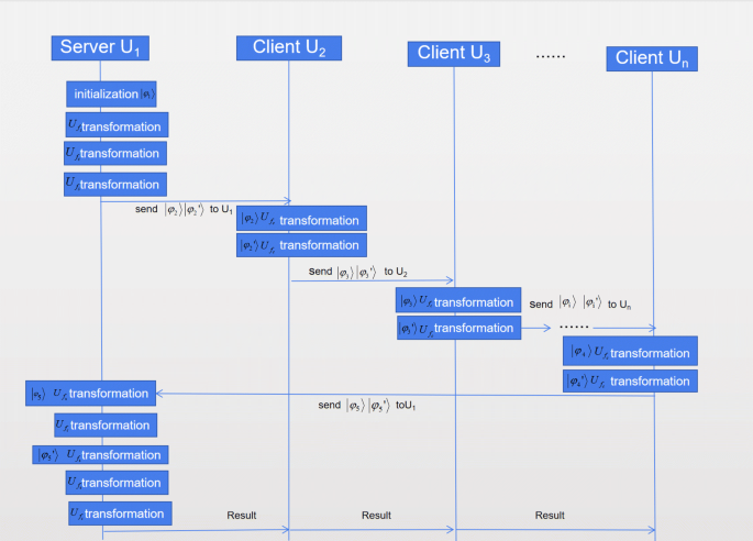
Sequence diagram
Let \(|\varphi _{2}\rangle =\frac {1}{\sqrt {N}}{\sum }_{x=0}^{N-1}|x\rangle |r\oplus {f_{A_{1}}(x)}\rangle \). ⊕ is the operator of module 2. Then, we do the same transformation \(U_{f_{s}}\) on |φ2〉⊗|1〉, as follow:
$$ U_{f_{s}}:|\varphi_{2}\rangle|1\rangle\to\frac{1}{\sqrt{N}}\sum\limits_{x=0}^{N-1}|x\rangle|r\oplus{f_{A_{1}}(x)}\oplus{1}\rangle\\ $$(16)Let \(|\varphi _{2}^{\prime }\rangle =\frac {1}{\sqrt {N}}{\sum }_{x=0}^{N-1}|x\rangle |r\oplus {f_{A_{1}}(x)}\oplus {1}\rangle \). Then the server U1 sends |φ2〉, \(|\varphi _{2}^{\prime }\rangle \) to the client U2 through the quantum channel.
- Step3.:
-
When the client U2 received the state |φ2〉, \(|\varphi _{2}^{\prime }\rangle \), then the client U2 will do another transformation \(U_{f_{c}}\) on state |φ2〉, the transformation \(U_{f_{c}}\)is defined as follow:
$$ f_{A_{2}}(x)= \left\{\begin{array}{ll} 1&if{x\in{A_{2}}}\\ 0&if{x\notin{A_{2}}} \end{array}\right. $$(17)$$ U_{f_{c}}:\frac{1}{\sqrt{N}}\sum\limits_{x=0}^{N-1}|x\rangle|r\otimes{f_{A_{1}}}(x)\rangle|f_{A_{2}}(x)\rangle\to\\ \frac{1}{\sqrt{N}}\sum\limits_{x=0}^{N-1}|x\rangle|(r\oplus{f_{A_{1}}(x)})\times{f_{A_{2}}(x)}\rangle\\ $$(18)

Here, Let \(|\varphi _{3}\rangle =\frac {1}{\sqrt {N}}{\sum }_{x=0}^{N-1}|x\rangle |(r\oplus {f_{A_{1}}(x)})\times {f_{A_{2}}(x)}\rangle ,\times \) is an operator that is logical multiplication. Then does the transformation \(U_{f_{c}}\) on \(|\varphi _{2}^{\prime }\rangle \) as follow:
Let \(|\varphi _{3}^{\prime }\rangle =\frac {1}{\sqrt {N}}{\sum }_{x=0}^{N-1}|x\rangle |(r\oplus {f_{A_{1}}(x)}\oplus 1)\times {f_{A_{2}}(x)}\rangle \). Then client U2 sends |φ3〉, \(|\varphi _{3}^{\prime }\rangle \) to the client U3 through the quantum channe2.
- Step4.:
-
After client U3 receives \(|\varphi _{3}\rangle ,|\varphi _{3}^{\prime }\rangle \), the client U3 does the same transformation \(U_{f_{c}}\) on state |φ3〉. then we get the result:
$$ U_{f_{c}}(\varphi_{3}):\frac{1}{\sqrt{N}}\sum\limits_{x=0}^{N-1}|x\rangle|(r\oplus{f_{A_{1}}(x)})\times{f_{A_{2}}(x)}\times{f_{A_{3}}(x)}\rangle\\ $$(20)Here, we use state \(U_{f_{c}}(|\varphi _{3}\rangle )\) to expressed the results. Then the client U3 does \(U_{f_{c}}\) transformation on \(|\varphi _{3}^{\prime }\rangle \). The result is \(U_{f_{c}}(|\varphi _{3}^{\prime }\rangle )=\frac {1}{\sqrt {N}}{\sum }_{x=0}^{N-1}|x\rangle |(r\oplus {f_{A_{1}}(x)}\oplus 1) \times {f_{A_{2}}(x)}\times {f_{A_{3}}(x)}\rangle \)
Then send \(U_{f_{c}}(|\varphi _{3}\rangle )\), \(U_{f_{c}}(|\varphi _{3}^{\prime }\rangle )\) to the client U4 through the quantum channe3, after the client U4 receives \(U_{f_{c}}(|\varphi _{3}\rangle )\), \(U_{f_{c}}(|\varphi _{3}^{\prime }\rangle )\), and does \(U_{f_{c}}\) transformation on \(U_{f_{c}}(|\varphi _{3}\rangle )\), \(U_{f_{c}}(|\varphi _{3}^{\prime }\rangle )\) respectively, then send the results to the next client and until the last client Un, the last client Un does \(U_{f_{c}}\) transformation respectively, uses |φ〉, \(|\varphi ^{\prime }\rangle \) as the last results which will be sent to the server U1.
- Step5::
-
when the server U1 receives the state |φ〉, it will do the transformation \(U_{f_{s}}\) on |φ〉×|r〉.
$$ \begin{array}{@{}rcl@{}} U_{f_{s}}(\varphi)&=&\frac{1}{\sqrt{N}}\sum\limits_{x=0}^{N-1}|x\rangle|(r\oplus{f_{A_{1}}(x)})\\ &&\times{f_{A_{2}}(x)} \times{\dots} \times{f_{A_{n}}(x)}\oplus{r}\rangle \end{array} $$(21)Then does \(U_{f_{c}}\) on state \(U_{f_{s}}(|\varphi \rangle )\)
$$ \begin{array}{@{}rcl@{}} U_{f_{c}}(U_{f_{s}}(\varphi))=\frac{1}{\sqrt{N}}\sum\limits_{x=0}^{N-1}|x\rangle|[(r\oplus{f_{A_{1}}(x)})\\ \times{f_{A_{2}}(x)} \times\dots \times{f_{A_{n}}(x)}\oplus{r}]\times{f_{A_{1}}(x)}\rangle \end{array} $$(22)
Let \(|\varphi _{4}\rangle =\frac {1}{\sqrt {N}}{\sum }_{x=0}^{N-1}|x\rangle |[(r\oplus {f_{A_{1}}(x)})\times {f_{A_{2}}(x)} \times \dots \times {f_{A_{n}}(x)}\oplus {r}]\times {f_{A_{1}}(x)}\rangle \) When the server U1 receives the state \(|\varphi ^{\prime }\rangle \), it will do two \(U_{f_{s}}\) transformation on \(|\varphi ^{\prime }\rangle \)
Let\(|\varphi _{4}^{\prime }\rangle =\frac {1}{\sqrt {N}}{\sum }_{x=0}^{N-1}|x\rangle |(r\oplus {f_{A_{1}}(x)}\oplus 1)\times {f_{A_{2}}(x)} \times \dots \times {f_{A_{n}}(x)}\oplus {r}\oplus {f_{A_{1}}(x)}\rangle \).
- Step6::
-
Then the server U1 does Uf transformation on \(|\varphi _{4}^{\prime }\rangle \) and |φ4〉. Then get
$$ \begin{array}{@{}rcl@{}} |\varphi_{5}\rangle&=& \frac{1}{\sqrt{N}}\sum\limits_{x=0}^{N-1}|x\rangle |[(r\oplus{f_{A_{1}}(x)})\times{f_{A_{2}}(x)} \times\dots\\ &&\times{f_{A_{n}}(x)}\oplus{r}\oplus{f_{A_{1}}(x)}]\times\sim\rangle \end{array} $$(25)where \(\sim = |[(r\oplus {f_{A_{1}}(x)}\oplus 1)\times {f_{A_{2}}(x)} \times {\dots } \times {f_{A_{n}}(x)}\oplus {r}\oplus {f_{A_{1}}(x)}]\rangle \), and \(|[(r\oplus {f_{A_{1}}(x)})\times {f_{A_{2}}(x)} \times {\dots } \times {f_{A_{n}}(x)}\oplus {r}\oplus {f_{A_{1}}(x)}]\times \sim \rangle \) contains the classical information about the cardinality of their intersection.
- Step7::
-
The state |φ5〉 carried the cardinality of their intersection, so we should extract the intersection cardinality from |φ5〉, the server U1 prepares quantum state \(\frac {1}{\sqrt {M}}{\sum }_{y=0}^{M-1}|y\rangle \), M is a big integer, so the value of \(\frac {2\pi }{\sqrt {t(N-t)}}+\frac {\pi ^{2}}{M^{2}}|N-2t|\) is very small (t is defined in Step8). Let \(|\varphi _{6}\rangle =\frac {1}{\sqrt {M}}{\sum }_{y=0}^{M-1}|y\rangle \otimes |\varphi _{5}\rangle \). Then, the server U1 does a quantum operator CF on |φ6〉, the result is state |φ7〉, CF is the following:
$$ C_{F}:|\varphi_{6}\rangle\to|\varphi_{7}\rangle $$$$ C_{F}:\frac{1}{\sqrt{M}}\sum\limits_{y=0}^{M-1}|y\rangle\otimes|\varphi_{5}\rangle\to \frac{1}{\sqrt{M}}\sum\limits_{y=0}^{M-1}|y\rangle\otimes{G^{y}}|\varphi_{5}\rangle $$(26)$$ \begin{array}{@{}rcl@{}} &&|\varphi_{7}\rangle= \frac{1}{\sqrt{M}}\sum\limits_{y=0}^{M-1}|y\rangle\otimes{G^{y}}|\varphi_{6}\rangle= \frac{1}{\sqrt{M}}\sum\limits_{y=0}^{M-1}|y\rangle\otimes{G^{y}}\\ &&\frac{1}{\sqrt{N}}\sum\limits_{x=0}^{N-1}|x\rangle |[(r\oplus{f_{A_{1}}(x)})\times{f_{A_{2}}(x)} \times\dots \times{f_{A_{n}}(x)}\\ &&\oplus{r}\oplus{f_{A_{1}}(x)}]\times\sim\rangle \end{array} $$(27)G is defined by \(G=U_{\varphi _{6}}U_{f_{r}}\), G is an operator of amplitude amplification .
$$ U_{f_{r}}|x\rangle|r\rangle= \left\{\begin{array}{ll} -|x\rangle|1\rangle&if {r=1}\\ |x\rangle|0\rangle&if {r=0} \end{array}\right. $$(28)$$ U_{\varphi_{6}}=2|\varphi_{6}\rangle\langle\varphi_{6}|-I $$(29)I is the identity operator.
- Step8::
-
The server U1 does QFT− 1 on the first logM qubits of |φ7〉 and then measures the first logM qubits to obtain |x〉, and outputs \(Nsin^{2}(\frac {x}{M}\pi )\) as the estimation of t, t is the number of the items that the last one qubit of |φ6〉 is in |1〉, for example, just like |x〉|1〉 in |φ6〉. If \(t<\frac {N}{2}\), then server U1 outputs \(\frac {{\sum }_{i=1}^{n}n_{c_{i}}-t}{2}\), means, \(|A_{1}\cap {A_{2}}\cap \dots \cap {A_{n}}|=\frac {{\sum }_{i=1}^{n}n_{c_{i}}-t}{2}\); otherwise \(\frac {(n_{c}+n_{s}+t)-N}{2}\), means, \(|A_{1}\cap {A_{2}}\cap \dots \cap {A_{n}}|=\frac {(n_{c}+n_{s}+t)-N}{2}\).
- Step9::
-
The server sends the result t to all the clients.
If we want to whether someone is intercepting in the channel, the bait technology can be used. That is, when qubit sequence are transmitted, the sender randomly inserts some bait particles which is prepared randomly with either Z-basis (i.e.,{|0〉,|1〉} or X-basis (i.e.,\(\{\frac {1}{\sqrt 2}+|1\rangle ,\frac {1}{\sqrt 2}-|1\rangle \}\). When the receiver received the sequence, the sender would public the bait particles positions and the measurement basis. Then the receiver’s measures the bait particles accord to the public and tells his measurement results to the sender. The sender compares the receiver results with the bait particles of the initial and then analyzes it. If the error is too much according to the channel noise, then drop the protocol and restart transmitting. Otherwise, it will continue to proceed next step.
4 Analysis
Let’s proof the correctness. Based on the state \(|\varphi _{5}\rangle = \frac {1}{\sqrt {N}}{\sum }_{x=0}^{N-1}|x\rangle |[(r\oplus {f_{A_{1}}(x)})\times {f_{A_{2}}(x)} \times \dots \times {f_{A_{n}}(x)}\oplus {r}\times {f_{A_{1}}(x)}]\times \sim \rangle \), \([(r\oplus {f_{A_{1}}(x)})\times {f_{A_{2}}(x)} \times \dots \times {f_{A_{n}}(x)}\oplus {r}\times {f_{A_{1}}(x)}]\times \sim \) is 0 or 1, so we define
Then we know that the state |φ5〉 can be re-expressed by (32)
Equation (32) means that |φ5〉 is the uniform superposition of all product states, |α〉 is the uniform superposition of these product states satisfying \([(r\oplus {f_{A_{1}}(x)})\times {f_{A_{2}}(x)} \times {\dots } \times {f_{A_{n}}(x)}\oplus {r}\times {f_{A_{1}}(x)}]\times \sim =1\) and β is opposite of α, means \([(r\oplus {f_{A_{1}}(x)})\times {f_{A_{2}}(x)} \times {\dots } \times {f_{A_{n}}(x)}\oplus {r}\times {f_{A_{1}}(x)}]\times \sim =0\). Obviously, α ⊥ β. if we choose \(\theta \in (0,\frac {\pi }{2})\), \(sin^{2}\theta =\frac {t}{N}\). then \(sin\theta =\sqrt {\frac {t}{N}}\), \(cos\theta =\sqrt {\frac {N-t}{N}}\), and thus |φ4〉 = cos|β〉 + sin|α〉. Then , we can get the following equations:
In the two-dimensional subspace, G is a rotation operator of angle 2𝜃 oriented from |β〉 to |α〉 spanned by |α〉 and |β〉. From |φ6〉, apply G and rotate it toward |α〉 by 2𝜃. Reapply G and rotate it close to |α〉. Moreover, there are two orthogonal states defined in the following:
|ϕ+〉 and |ϕ−〉 are eigenvectors of G, ei2𝜃and e−i2𝜃 are eigenvalues, respectively. Let 𝜃 = πω, then \(|\varphi _{6}\rangle =cos|\beta \rangle +sin|\alpha \rangle = \frac {e^{i\pi \omega }}{\sqrt 2}|\phi _{+}\rangle +\frac {e^{-i\pi \omega }}{\sqrt 2}|\phi _{-}\rangle \).If we apply G rotation operator to |φ6 for y times, then
Then, we can get
then applying QFT− 1 to the first logM qubits of |φ8〉, we can get
with
Make a measurement on \(|\widetilde {x}_{+}\rangle \) in the computational basis \(\{|0\rangle ,|1\rangle ,\dots ,|M-1\rangle \}\) then get |x〉 with the probability \(|\frac {1}{M}{\sum }_{y=0}^{M-1}e^{i2\pi {y}(\omega -\frac {x}{M})}|^{2}\). so,
After measuring, \(\frac {x}{M}\) is close to or equal to ω with high probability. In fact, when make a measurement on \(|\widetilde {x}_{+}\rangle \), the probability of getting either ⌊Mω⌋ or ⌈Mω⌉ is at least \(\frac {8}{\pi ^{2}}\), with the estimation ω within the error \(\frac {1}{M}\). Similarly, make a measurement on \(|\widetilde {x}_{-}\rangle \), the probability of getting either ⌊M(1 − ω)⌋ or ⌈M(1 − ω)⌉ is at least \(\frac {8}{\pi ^{2}}\), with the estimation 1 − ω within the error \(\frac {1}{M}\), so \(\frac {x}{M}\) is close to or equal to 1 − ω with high probability. For 𝜃 = πω and \(sin^{2}\theta =\frac {t}{N}\), t = Nsin2πω.For the first case (i.e.,\(|\widetilde {x}_{+}\rangle \) ), \(\omega =\frac {x}{M}\), so \(t=Nsin^{2}(\pi \frac {x}{M})\);for the second case (i.e,\(|\widetilde {x}_{-}\rangle \) ),\(\omega \approx 1-\frac {x}{M}\), so \(t=Nsin^{2}(\pi -\pi \frac {x}{M})=Nsin^{2}(\pi \frac {x}{M})\).For the two cases, get the same estimation t.
Theorem 1 [16]. For \(\forall {M}\in {Z},|t-\widetilde {t}|\le \frac {2\pi }{M}\sqrt {t(N-t)}+\frac {\pi ^{2}}{M^{2}}|N-2t|\), the least probability is \(\frac {8}{\pi ^{2}}\),so \(\widetilde {t}\) is an estimate of t. the error is \(\varepsilon \le \frac {2\pi }{M}\sqrt {t(N-t)}+\frac {\pi ^{2}}{M^{2}}|N-2t|\).
Then we know the relations between t and \(|A_{1}\cap {A_{2}}\cap \dots \cap {A_{n}}|\)
In Step 8, we can get the estimation of t with the high probability p, and \(p\ge \frac {8}{\pi _{2}}\), error is ε, error is very small, and \(\varepsilon \le \frac {2\pi }{M}\sqrt {t(N-t)}+\frac {\pi ^{2}}{M^{2}}|N-2t|\); so the QSMS-IC protocol can get the estimation of \(|A_{1}\cap {A_{2}}\cap \dots \cap {A_{n}}|\) with high probability \(p\ge \frac {8}{\pi _{2}}\) and small error ε.
Then analyze the security.
Theorem 2 (client Privacy). In QSMS-IC protocol, the client Ui can not get the information about the elements of A1 except the set size, and the server U1 also can not get the information about the elements of Ai except the set size.
Proof. In QSMS-IC protocol, the server U1 sends a quantum state |φ2〉 to the server U2, without revealing the elements of the set. Though the state |φ2〉 including the information of \(f_{A_{1}}(x)\), the client U2 cannot extract \(f_{A_{1}}(x)\) from |φ2〉. Supposed that the quantum state |φ2〉 consists of two subsystems: the n-qubit system \(\widetilde {C}\) and the 1-qubit system \(\widetilde {S}\), \(\widetilde {S}\) is ancillary system. Suppose the clients are half a honest client which is curious about other client’s information and actually transmits personal information. The client makes a projective measurement on |φ2〉, it can get \(|x\rangle |r\oplus {f_{A_{1}}(x)}\rangle \) with probability\(\frac {1}{n}\). Thus, \(\widetilde {S}\) can be characterized by quantum ensemble \(\xi \equiv \{p_{x}, \rho _{\widetilde {S}}(x)\}\), and \(p_{x}=\frac {1}{n}\),
For \(|\varphi _{2}\rangle =\frac {1}{N}{\sum }_{x=0}^{N-1}|x\rangle |r\oplus {f_{A_{1}}(x)}\rangle \), so \(\widetilde {S}\) can also be described by the following density operator,
Thus, \(\rho _{\widetilde {S}}\) is the average state of \(\widetilde {S}\). based on Holevo bound [14], we can get
Get the maximum value at \(t=\frac {N}{2}\). namely
It is the upper bound that the clients can get from \(\widetilde {S}\) through the measurement. But the client U2 does not know the random r which is selected by the server U1, so H(r) = 1 (H(.)is Shannon entropy and S(.)is Von Neumann entropy). Namely, it encrypts \(f_{A_{1}}(x)\) by using the random R in one-time pad method. So, from |φ2〉, U2 cannot get the information of \(f_{A_{1}}(x)\).
In addition, if the client does not honestly execute this protocol, he can send a fake state |X〉to the server, instead of the state |φ1〉. Accordingly, the returned state from the server will be \(|x\rangle |r\oplus {f_{A_{1}}(x)}\rangle \), not |φ2〉. Due to the random number r obviously the client can still not get any information about \(f_{A_{1}}(x)\).
So, the client Ai can’t get the information of \(f_{A_{1}}(x)\), due to the random r. Therefore, in QSMS-IC protocol, the client Ai can’t get the set elements of A1 except the set size \(n_{c_{i}}\). similarly the client A1 also can’t get the information of the elements of Ai set except the set size.
5 Conclusion
In this paper, we proposed a protocol called Quantum Secure Multiparty Set Intersection Cardinality Protocol to privately compute the cardinality of set intersection. Unlike the classical PSI-CA protocols, the proposed QSMS-IC protocol achieves the unconditional security, because it is guaranteed by the basic principle of quantum mechanics; compared with quantum PSI-CA protocol for two-party set Intersection, the proposed protocol can achieve multi-party set intersection. In addition, our proposed scheme is very simple to deal with dynamic updating, because it only needs to compute some set operations if adding or deleting a new client. What’s more, the applications of the protocol is frequently used in large-scale social networks, for instance, users can privately calculate the common hobbies.
References
Vu, D.H., Luong, D., Ho, T.B.: An Eefficient approach for secure multi-party computation without authenticated channel, Information Sciences online (2019)
Zhao, C., Zhao, S.N., Zhao, M.H., Chen, Z.X., Gao, C.Z., Li, H.W., Tan, Y.A.: Secure multi-party computation: Theory, practice and applications. Inform. Sci. 476, 357–372 (2019)
Wang, Z., Cheung, S.C.S., Luo, Y.: Information theoretic secure multi-party computation with collusion deterrence. IEEE Trans. Inf. Forensi. Secur. 4(12), 980–995 (2017)
Xu, L., bao, T., Zhu, L.H., Zhang, Y.: Trust-based privacy-preserving photo sharing in online social networks. IEEE Trans. Multimed. 21(3), 591–602 (2019)
Xiong, H., Zhang, H., Sun, J.F.: Attribute-based privacy-preserving data Sharing for dynamic groups in cloud computing. IEEE Syst. J. 3(13), 2739–2750 (2019)
Shi, R.H., Mu, Y., Zhong, H., Cui, J., Zhang, S.: An efficient quantum scheme for private set intersection. Quantum Inf. Process 1(15), 363–371 (2016)
Shi, R.H.: Quantum private computation of cardinality of set intersection and union, European Physical Journal. vol.12(72) (2018)
Shi, R.H., Mu, Y., Zhong, H., Zhang, S., Cui, J.: Quantum private set intersection cardinality and its application to anonymous authentication. Inform. Sci. 370-371, 147–158 (2016)
Wen, Y.M., Gong, Z., Huang, Z.G., Qiu, W.D.: A new efficient authorized private set intersection protocol from Schnorr signature and its applications. Cluster Comput. J. Netw. Soft. Tools Appl. 1, 287–297 (2018)
Shi, R.H.: Efficient quantum protocol for private set intersection cardinality. IEEE Access 6, 73102–73109 (2018)
Cristofaro, E.D., Gasti, P., Tsudik, G.: Fast and private computation of cardinality of set intersection and union, cryptology and network security (CANC 2010), Springer. LNCS 7712, 218–231 (2012)
Debnath, S.K., Dutta, R.: New realizations of efficient and secure private set intersection protocols preserving fairness. Inf. Secur. Crypt. 10157, 254–284 (2017)
Kissner, L., Song, D.: Privacy-preserving set operations. In: Proc. advances in cryptology - Crypto 2005, Springer, LNCS 3621, pp. 241–257 (2005)
Grover, L.K.: A fast quantum mechanical algorithm for database search. In: Proc. 28th annual ACM symposium on theory of computing, ACM, pp. 212–219 (1996)
Buccafurri, F., Fotia, L., Lax, G., Saraswat, V.: Analysis-preserving protection of user privacy against information leakage of social-network likes. Inf. Sci. 328, 340–358 (2016)
Nielsen, M.A., Chuang, I.L.: Quantum computation and quantum information. Cambridge University Press, Cambridge (2010)
Boyer, M., Brassard, G., Hyer, P., Tapp, A.: Tight bounds on quantum searching Fortschritte der Physik 4-5(46), 493–505 (1998)
Carminati, B., Ferrari, E., Guglielmi, M.: Detection of unspecified emergencies for controlled information sharing. IEEE Trans. Dependable Secure Comput. 6(13), 630–643 (2016)
Xu, J., Schaar, M.V.D.: Efficient working and shirking in information sharing networks. IEEE J. Select. Areas Commun. 4(33), 651–662 (2015)
Wang, X.A., Fatos, X.F., Luo, X.S., Zhang, S.W., Yong, D.: A privacy-preserving fuzzy interest matching protocol for friends finding in social networks. Soft Compu. 8(22), 2517–2526 (2018)
Wu, M.E., Chang, S.Y., Lu, C.J., Sun, H.M.: A communicationefficient private matching scheme in Client-Server model. Inf. Sci. 275, 348–359 (2014)
Diao, Z.J., Huang, C.F., Wang, K.: Quantum counting: Algorithm and error distribution. Acta Appl. Math. 118, 147–159 (2012)
Shi, R.H., Zhang, S.: Quantum solution to a class of two-party private summation problems. Quantum Inf. Process. 16, 225 (2017)
Vaidya, J., Shafiq, B., Fan, W., Mehmood, D., Lorenzi, D.: A random decision tree framework for privacy-preserving data mining. IEEE Trans. Dependable Secure Comput. 11, 399–411 (2014)
Yao, A.: Protocols for secure computations, in Proc. 23th Annu, Symp. Found. Comput. Sci. (FOCS), pp. 160–164 (1982)
Narayanan, A., Thiagarajan, N., Lakhani, M., Hamburg, M., Boneh, D.: Location privacy via private proximity testing, in Proc. Netw. Distrib. Syst. Secur, Symp., Online (2011)
Wang, Q., Shi, R., Chen, Z., Wang, S.: A Quantum sealed auction protocol based on secret sharing. Int. J. Theor. Phys. 58, 1128–1137 (2019)
Zhang, S., Wang, S., Wang, Q., Shi, R.: Quantum anonymous voting protocol with the privacy protection of the candidate. Int. J. Theor. Phys. 58, 3323–3332 (2019)
Xu, G., Zou, X.: Security analysis of an arbitrated quantum signature scheme with bell states. Int. J. Theor. Phys. 55(9), 1–15 (2016)
Chen, Y., Chou, J., Zhou, F.: A publicly verfiable quantum signature scheme based on asymmetruc quantum crytography. IACR Crypology e Print Archive 2019, 24 (2019)
Author information
Authors and Affiliations
Corresponding author
Additional information
Publisher’s Note
Springer Nature remains neutral with regard to jurisdictional claims in published maps and institutional affiliations.
Manuscript received Nov xx, 2019; revised xx–xx, xxxx. This work was supported by the National Natural Science Foundation of China (No.61672010, No.61702168 and No.61701173), Ph. D. Programs Foundation(BSQD2019024), Provincial education project(B2018310)
Rights and permissions
Open Access This article is licensed under a Creative Commons Attribution 4.0 International License, which permits use, sharing, adaptation, distribution and reproduction in any medium or format, as long as you give appropriate credit to the original author(s) and the source, provide a link to the Creative Commons licence, and indicate if changes were made. The images or other third party material in this article are included in the article's Creative Commons licence, unless indicated otherwise in a credit line to the material. If material is not included in the article's Creative Commons licence and your intended use is not permitted by statutory regulation or exceeds the permitted use, you will need to obtain permission directly from the copyright holder. To view a copy of this licence, visit http://creativecommons.org/licenses/by/4.0/.
About this article

Cite this article
Liu, B., Zhang, M. & Shi, R. Quantum Secure Multi-party Private Set Intersection Cardinality. Int J Theor Phys 59, 1992–2007 (2020). https://doi.org/10.1007/s10773-020-04471-8
Received:
Accepted:
Published:
Issue Date:
DOI: https://doi.org/10.1007/s10773-020-04471-8