All congruences below stability-preserving fair testing or CFFD

Abstract

In process algebras, a congruence is an equivalence that remains valid when any subsystem is replaced by an equivalent one. Whether or not an equivalence is a congruence depends on the set of operators used in building systems from subsystems. Numerous congruences have been found, differing from each other in fine details, major ideas, or both, and none of them is good for all situations. The world of congruences seems thus chaotic, which is unpleasant, because the notion of congruence is at the heart of process algebras. This study continues attempts to clarify the big picture by proving that in certain sub-areas, there are no other congruences than those that are already known or found in the study. First, the region below stability-preserving fair testing equivalence is surveyed using an exceptionally small set of operators. The region contains few congruences, which is in sharp contrast with an earlier result on the region below Chaos-Free Failures Divergences (CFFD) equivalence, which contains 40 well-known and not well-known congruences. Second, steps are taken towards a general theory of dealing with initial stability, which is a small but popular detail. This theory is applied to the region below CFFD.

1 Introduction

This study is motivated by a striking difference: in the case of sequential computation, the notion of the result of a computation at the highest level of abstraction is simple, clear and widely agreed upon, whereas in the case of concurrent computation, many alternatives are widely used and numerous more alternatives are known to exist. Let us discuss this a bit.

It is universally agreed that a deterministic sequential program computes a partial function. The function is partial, because with some inputs the program may fail to terminate. This nice picture is slightly complicated by the fact that sequential programs may contain intentional nondeterminism, such as in the Miller–Rabin probabilistic primality test [1, 13]; or unwanted nondeterminism, such as in i=i++ + 1; (a Wikipedia example of undefined behavior).¹ This issue could be taken into account by declaring that a sequential program executes a relation from the set of inputs to the set of outputs union $\{\perp \}$: (i, o) is in the relation if and only if, for the input i, o is a possible output or $o = \perp$ denoting failure to terminate. These abstract views to sequential programs are simple, natural, and widely accepted. At their level of abstraction, they have no rivals.

The situation is entirely different with concurrent programs. A concurrent program computes a behaviour. Behaviours may be—and have been—compared with branching bisimilarity [8], weak bisimilarity [10], CSP failures divergences equivalence [15], Chaos-Free Failures Divergences (CFFD) equivalence [20], and numerous other equivalences. None of them is widely considered as the “most natural” or “right” notion of “similar behaviour”. If there is any agreement, it is that the choice of the most appropriate equivalence depends on the situation. Even the same users keep on switching between different equivalences depending on the task at hand, such as in [15], where, for instance, stable failures equivalence is used when the so-called catastrophic divergence phenomenon prevents the use of failures divergences equivalence.

The famous survey [5], among others, has improved our understanding a lot by presenting many equivalences in a systematic framework. However, such surveys do not provide full information, because they only discuss known equivalences. They leave it open whether there could be unknown useful equivalences with interesting properties.

In many situations the equivalence must be a congruence with respect to the operators that are available for building systems from subsystems. This requirement is so strong that it makes it possible to survey certain regions of equivalences, list all congruences in them, and prove that they contain no other congruences. Chapters 11 and 12 of [15] survey two regions and prove that there are three congruences in each. In [17], all congruences that are implied by the CFFD equivalence were found. This fairly large region contains 40 congruences, including stable failures equivalence, CSP failures divergences equivalence, and trace equivalence. Five kinds of failures, four kinds of infinite traces, two kinds of divergence traces, and two kinds of traces were needed, some of them new. Perhaps none of the previously unknown congruences among the 40 is interesting, but if so, then we know that no interesting congruences are lurking in that region.

A task that is somewhat similar in spirit to fully surveying a region is to choose a property such as deadlock-freedom and find the weakest congruence that preserves the property. Such results have been published in, e.g., [2, 4, 6, 7, 9, 11, 12, 14, 16]. As explained in [17], knowing the weakest congruence helps in designing compositional verification algorithms for the property.

The congruence property depends on the set of operators for building systems. Perhaps the most well known example of this deals with the common choice operator “$+$”. Branching bisimilarity, weak bisimilarity, CSP failures divergences equivalence, CFFD equivalence, and many other equivalences are not congruences with respect to it. In CSP, the congruence property was obtained by rejecting the common choice operator and introducing two other choice operators instead. In most other theories, the common choice operator was kept and the equivalence was refined so that it became a congruence.

At this point it is worth mentioning that if we are only interested in so-called safety properties of systems (that is, whatever the system does must be acceptable), then there is a single very widely agreed “right” congruence: trace equivalence. Furthermore, it was proven in [18] that any operator that satisfies a rather natural weak assumption can be constructed from parallel composition and hiding modulo trace equivalence, implying that trace equivalence is a congruence with respect to every “reasonable” operator. This situation is comparable to sequential programs in simplicity and clarity.

Things become problematic indeed, when also so-called liveness properties are of interest (the system must eventually do something useful, or at least not lose the ability to nondeterministically choose to eventually do something useful). The problems are so severe that they have led to wide adoption of an equivalence that does not imply trace equivalence, that is, CSP failures divergences equivalence.

The above-mentioned results in [15] use a fairly large set of operators. In particular, they use a “throw” operator that rules out many equivalences that would otherwise be congruences. The results in [17] only use parallel composition, hiding, relational renaming, and action prefix. Therefore, where the regions considered by [15] and [17] overlap, [17] gives additional congruences.

In [19], of which the present study is an extension, all congruences were found that are implied by the stability-preserving fair testing equivalence of [14]. This equivalence is a congruence. It is interesting for many reasons. It is the weakest congruence that preserves the property AGEFa, that is, “in all futures always, there is a future where eventually a occurs”. It offers an alternative approach to the verification of liveness properties. With the traditional approach, it is often necessary to explicitly state so-called fairness assumptions, which may be a burden. With fair testing equivalence this is unnecessary, because, so to speak, it has a built-in fairness assumption that is acceptable in many cases. Unlike other congruences for a significant subset of liveness properties, it has a very well-working partial order reduction method [21]. On the theoretical side, its definition is an interesting exception, because it seems somewhat ad-hoc instead of following a familiar pattern.

An important feature of [19] is that only parallel composition, hiding, and functional renaming were used for proving the absence of more congruences. This is a strictly smaller set of operators than in [15] and [17]. In [17] it was proven that if a congruence is implied by strong bisimilarity (this is a very weak assumption) and preserves anything, then it preserves at least the alphabet. It was shown with two counter-examples that the result depends on the availability of the action prefix and relational renaming operators. In [19], one of the counter-examples was encountered again, and six new (albeit uninteresting) congruences were found that do not preserve the alphabet.

The most important finding of [19] was that there is only one congruence between the not stability-preserving fair testing equivalence and the congruence that only preserves the alphabet: trace equivalence. If one wants to have something like fair testing, then one must go all the way to fair testing. There are no intermediate stops. This is in sharp contrast to [17]. It is also somewhat surprising, because the definition of fair testing seems quite ad-hoc, and because fair testing preserves AGEFa which is a well-known example of a property that is not linear-time (e.g., [3, p. 32]). The importance of this result is strengthened by the fact that it was obtained in the presence of only parallel composition, hiding, and functional renaming. Also this is different from [17].

A widely used way to make an equivalence a congruence with respect to the common choice operator is to add information on initial stability: systems that can initially execute an invisible action are deemed inequivalent to systems that cannot. The study [19] was the first one that fully covers a region induced by a stability-preserving congruence. Also the weakest stability-preserving congruence was found. Some unexpected or at least unconventional congruences were found, but they may be considered uninteresting, because they rely on the absence of the action prefix operator.

The present study makes two contributions. First, the conference paper [19] had a strict page limit, leading to dense proofs that are hard to read. The present study attempts to make the results in [19] more readable. Second, it develops a theory that greatly simplifies the treatment of initial stability when proving the absence of unknown congruences, at the cost of assuming the congruence property with respect to more operators than [19]. Therefore, it gives less general results on fair testing equivalence than [19]. On the other hand, it applies to CFFD equivalence.

Section 2 presents the necessary background concepts. The congruences that are implied by stability-preserving fair testing equivalence are introduced in Sect. 3. In Sect. 4, the weakest stability-preserving congruence is found. That stability-preserving fair testing equivalence does not imply more congruences is proven in Sect. 5. The new theory on adding initial stability checking is presented in Sect. 6, and applied to CFFD equivalence in Sect. 7 resulting in 79 congruences. This study is concluded by a discussion section.

2 LTSs and their operators

In this section we list many widely known concepts needed in this study, pointing out little facts that are useful to remember when reading our proofs. We also pay attention to details that vary in the literature, discussing the motivation of our choice.

The empty string is denoted with $\varepsilon$. The set of strings on A is denoted with $A^*$, and $A^+ = A^* {\setminus } \{\varepsilon \}$. If $\pi$ and $\sigma$ are strings, then $\pi \sqsubseteq \sigma$ denotes that $\pi$ is a prefix of $\sigma$, that is, there is a string $\rho$ such that $\sigma = \pi \rho$. If $\pi$ is a string and K is a set of strings, then $\pi \sqsubseteq K$ denotes that there is $\sigma \in K$ such that $\pi \sqsubseteq \sigma$. We have $\varepsilon \sqsubseteq K$ if and only if $K \ne \emptyset$. We define $\pi ^{-1}K = \{ \rho \mid \pi \rho \in K \}$. It is nonempty if and only if $\pi \sqsubseteq K$. Trivially $\varepsilon ^{-1}K = K$.

The invisible action is denoted with $\tau$. It denotes the occurrence of something that the outside world does not see. This is different from the occurrence of nothing, thus $\tau \ne \varepsilon$. An alphabet is any set $\varSigma$ such that $\varepsilon \notin \varSigma$ and $\tau \notin \varSigma$. Its elements are called visible actions.

A labelled transition system or LTS is a tuple $(S, \varSigma , \varDelta , {\hat{s}})$ such that $\varSigma$ is an alphabet, $\varDelta \subseteq S \times (\varSigma \cup \{\tau \}) \times S$, and ${\hat{s}} \in S$. Elements of S and $\varDelta$ are called states and transitions, respectively, and ${\hat{s}}$ is the initial state. The transition $(s,a,s')$ may also be denoted with $s \mathrel {{-}a{\rightarrow }} s'$. By $s \mathrel {{-}a{\rightarrow }}$ we mean that there is $s'$ such that $s \mathrel {{-}a{\rightarrow }} s'$.

If an LTS is shown as a drawing, then, unless otherwise stated, its alphabet is the set of the visible actions along the transitions in the drawing. The alphabet may be specified explicitly in the text or near the bottom right corner of the drawing. For instance, the alphabet of is $\{a\}$ and the alphabet of is ${\{a,b\}}$. In particular, we will frequently use and , their alphabets being $\emptyset$.

In the constructions of this study, we will often need elements that are not in a given alphabet or in a given set of states. Such entities exist because, by the axiom of foundation in set theory, if X is a set, then X, $\{X\}$, $\{\{X\}\}$, and so on are not elements of X. Sometimes in the literature, instead of each LTS having an alphabet of its own, there is a single global alphabet. That convention would make things difficult in the present study, because elements that are not in the alphabet would not be available. We will return to this issue in Sect. 8.

We use L, M, $L'$, $M'$, $L_1$, $M_1$, and so on to denote LTSs. Unless otherwise stated, $L = (S, \varSigma , \varDelta , {\hat{s}})$, $L' = (S', \varSigma ', \varDelta ',$${\hat{s}}')$, $L_1 = (S_1, \varSigma _1, \varDelta _1, {\hat{s}}_1)$, and so on. Because this convention is sometimes unclear, we also use $\varSigma (L)$ to denote the alphabet of L. By $s \mathrel {{-}a{\rightarrow }}_i s'$ we mean that $(s,a,s') \in \varDelta _i$.

Researchers widely agree that at the detailed level, it is appropriate to compare behaviours using the following notion. Two LTSs $L_1$ and $L_2$ are bisimilar, denoted with $L_1 \equiv L_2$, if and only if $\varSigma _1 = \varSigma _2$ and there is a relation² “$\sim$” $\subseteq S_1 \times S_2$ with the following properties:

• 1. ${\hat{s}}_1 \sim {\hat{s}}_2$.

• 2. If $s_1 \mathrel {{-}a{\rightarrow }}_1 s'_1$ and $s_1 \sim s_2$, then there is $s'_2$ such that $s_2 \mathrel {{-}a{\rightarrow }}_2 s'_2$ and $s'_1 \sim s'_2$.

• 3. If $s_2 \mathrel {{-}a{\rightarrow }}_2 s'_2$ and $s_1 \sim s_2$, then there is $s'_1$ such that $s_1 \mathrel {{-}a{\rightarrow }}_1 s'_1$ and $s'_1 \sim s'_2$.

It is easy to check that if $L_1$ and $L_2$ are isomorphic, then they are bisimilar.

The reachable part of an LTS $(S, \varSigma , \varDelta , {\hat{s}})$ is $(S', \varSigma , \varDelta ', {\hat{s}})$, where $S'$ and $\varDelta '$ consist of those states and transitions to which there is a path from ${\hat{s}}$. Any LTS is bisimilar with its reachable part.

Next we define the six operators that this study will focus on.

Parallel composition$L_1 {\Vert }L_2$ It is the reachable part of $(S, \varSigma , \varDelta , {\hat{s}})$, where $S = S_1 \times S_2$, $\varSigma = \varSigma _1 \cup \varSigma _2$, ${\hat{s}} = ({\hat{s}}_1, {\hat{s}}_2)$, and $(s_1,s_2) \mathrel {{-}a{\rightarrow }} (s'_1,s'_2)$ if and only if

• $a \notin \varSigma _2$, $s_1 \mathrel {{-}a{\rightarrow }}_1 s'_1$, and $s'_2 = s_2 \in S_2$,

• $a \notin \varSigma _1$, $s_2 \mathrel {{-}a{\rightarrow }}_2 s'_2$, and $s'_1 = s_1 \in S_1$, or

• $a \in \varSigma _1 \cap \varSigma _2$, $s_1 \mathrel {{-}a{\rightarrow }}_1 s'_1$, and $s_2 \mathrel {{-}a{\rightarrow }}_2 s'_2$.

That is, if a belongs to the alphabets of both components, then an a-transition of the parallel composition consists of simultaneous a-transitions of both components. If a belongs to the alphabet of one but not the other component, then that component may make an a-transition while the other component stays in its current state. Also each $\tau$-transition of the parallel composition consists of one component making a $\tau$-transition without the other participating. The result of the parallel composition is pruned by only taking the reachable part.

It is easy to check that $L_1 {\Vert }L_2$ is isomorphic to (and thus bisimilar with) $L_2 {\Vert }L_1$, and $(L_1 {\Vert }L_2) {\Vert }L_3$ is isomorphic to $L_1 {\Vert }(L_2 {\Vert }L_3)$. This means that “${\Vert }$” can be considered commutative and associative.

Hiding$L {\setminus } A$ Let A be a set. The hiding of A in L is $(S, \varSigma ', \varDelta ', {\hat{s}})$, where $\varSigma ' = \varSigma {\setminus } A$ and $\varDelta ' = \{ (s,a,s') \in \varDelta \mid$$a \notin A \} \cup \{ (s,\tau ,s') \mid \exists a \in A: (s,a,s') \in \varDelta \}$. That is, labels of transitions that are in A are replaced by $\tau$ and removed from the alphabet. Other labels of transitions are not affected.

Relational renaming$L\varPhi$ Let $\varPhi$ be a set of pairs such that for every $(a,b) \in \varPhi$ we have $\tau \ne a \ne \varepsilon$ and $\tau \ne b \ne \varepsilon$. The domain of $\varPhi$ is $\mathcal {D}(\varPhi ) = \{ a \mid \exists b: (a,b) \in \varPhi \}$. Let the predicate $\varPhi (a,b)$ hold if and only if either $(a,b) \in \varPhi$ or $b = a \notin \mathcal {D}(\varPhi )$. The relational renaming of L with $\varPhi$ is $(S, \varSigma ', \varDelta ', {\hat{s}})$, where $\varSigma ' = \{ b \mid \exists a \in \varSigma : \varPhi (a,b) \}$ and $\varDelta ' = \{(s,b,s') \mid \exists a: (s,a,s') \in \varDelta \wedge \varPhi (a,b) \}$.

That is, $\varPhi$ renames visible actions to visible actions. A visible action may be renamed to more than one visible action. In that case, the transitions labelled by that action are duplicated as needed. If $\varPhi$ specifies no new names for an action, the transitions labelled by it remain unchanged. In particular, $\tau$-transitions remain unchanged. The alphabet of the result consists of the new names of the original visible actions where such have been defined, and of the remaining original visible actions as such. Pairs in $\varPhi$ whose first component is not in $\varSigma$ have no effect. This design makes it simple to specify the intended changes without causing accidental removal of the transitions that are not intended to change.

Functional renaming$\phi (L)$ Functional renaming is the subcase of relational renaming where $\varPhi$ specifies at most one new action name for each action. It is denoted with $\phi (L)$, where $\phi (a) = b$ if $(a,b) \in \varPhi$, and $\phi (a) = a$, otherwise. It is included in our list of six operators, because we will encounter some equivalences that are congruences with respect to it but not with respect to relational renaming.

We will frequently use the following two special cases of functional renaming as helpful notation in proofs. They attach and remove an integer i to visible actions. They will make it easy to ensure that in a parallel composition, precisely those actions synchronize whom we want to synchronize. In the notation, A is an alphabet, $\varepsilon \ne a \ne \tau$, and $\varepsilon \ne a_j \ne \tau$ for $1 \le j \le n$. Without loss of generality we assume that always $\varepsilon \ne a^{[i]} \ne \tau$.

$$\begin{aligned} \begin{array}{@{}rcl@{}} a^{[i]} &{} := &{} (a,i)\\ (a_1 a_2 \cdots a_n)^{[i]} &{} := &{} a_1^{[i]} a_2^{[i]} \cdots a_n^{[i]}\\ A^{[i]} &{} := &{} \{ a^{[i]} \mid a \in A\}\\ \lceil L\rceil ^{[i]} &{} := &{} L\varPhi ,\text { where }\varPhi = \{ (a,a^{[i]}) \mid a \in \varSigma \}\\ \lfloor L\rfloor _{[i]} &{} := &{} L\varPhi ,\text { where }\varPhi = \{ (a^{[i]},a) \mid a^{[i]} \in \varSigma \} \end{array} \end{aligned}$$

Action prefixa.L. Let $a \ne \varepsilon$. Let $\varSigma ' = \varSigma \cup \{a\}$ if $a \ne \tau$, and $\varSigma ' = \varSigma$ otherwise. The operator a.L yields $(S', \varSigma ', \varDelta ', {\hat{s}}')$, where ${\hat{s}}'$ is a new state (that is, ${\hat{s}}' \notin S$), $S' = S \cup \{{\hat{s}}'\}$, and $\varDelta ' = \varDelta \cup \{({\hat{s}}', a, {\hat{s}})\}$. That is, a.L starts by executing a, after which it is in the initial state of L.

Choice$L_1 + L_2$ Roughly speaking, the choice between $L_1$ and $L_2$ starts by executing an initial transition of $L_1$ or an initial transition of $L_2$. This transition represents a choice between $L_1$ and $L_2$. Then $L_1 + L_2$ continues like the chosen LTS continues after the corresponding transition.

This may be formalized by taking a disjoint union of $L_1$ and $L_2$, and adding a new state that acts as the initial state of the result. For each initial transition of $L_1$ and of $L_2$, a copy is made that starts at the new state. Indexing of state names is used to ensure that the union is disjoint. That is, $L_1 + L_2 = (S', \varSigma ', \varDelta ', {\hat{s}}')$, where $S' = S_1^{[1]} \cup S_2^{[2]} \cup \{{\hat{s}}'\}$, $\varSigma ' = \varSigma _1 \cup \varSigma _2$, $\varDelta ' = \varDelta '_1 \cup \varDelta ''_1 \cup \varDelta '_2 \cup \varDelta ''_2$, and ${\hat{s}}' \notin S_1^{[1]} \cup S_2^{[2]}$, where $\varDelta '_i = \{ (s^{[i]}, a, s'^{[i]}) \mid (s,a,s') \in \varDelta _i \}$ and $\varDelta ''_i = \{ ({\hat{s}}', a, s'^{[i]}) \mid ({\hat{s}}_i,a,s') \in \varDelta _i \}$ for $i \in \{1,2\}$.

Also “$+$” can be considered commutative and associative (up to bisimilarity).

Let “$\cong$” and “$\cong '$” be equivalences on LTSs. We say that “$\cong$” implies “$\cong '$” or “$\cong '$” is at least as weak as “$\cong$” if and only if “$\cong$” $\subseteq$ “$\cong '$”. This is equivalent to the following: for any LTSs $L_1$ and $L_2$ we have $L_1 \cong L_2 \Rightarrow L_1 \cong ' L_2$.

Let “$\cong$” be an equivalence on LTSs and $\mathsf {op}$ be a unary operator on LTSs. We say that “$\cong$” is a congruence with respect to$\mathsf {op}$ if and only if for every L and $L'$, $L \cong L'$ implies $\mathsf {op}(L) \cong \mathsf {op}(L')$. When we say that an equivalence is a congruence with respect to parallel composition, we mean that it is a congruence with respect to the two unary operators $\mathsf {op}_1(L) := L_1 {\Vert }L$ and $\mathsf {op}_2(L) := L {\Vert }L_2$. Because “${\Vert }$” is commutative, this is equivalent to saying that the equivalence is a congruence with respect to $\mathsf {op}_1(L)$. The similar convention and remark apply to “$+$”.

It is easy to show with induction that if $f(L_1, \ldots , L_n)$ is an expression, $L_i \cong L'_i$ for $1 \le i \le n$, and “$\cong$” is a congruence with respect to all operators used in f, then $f(L_1, \ldots , L_n) \cong f(L'_1, \ldots , L'_n)$.

3 Stability-preserving fair testing and the region below it

In this section we define 4 times 5 equivalences in a two-dimensional fashion. Stability-preserving fair testing equivalence is the strongest equivalence among them. We prove that 17 of these equivalences are congruences with respect to parallel composition, hiding, and functional renaming. We investigate the congruence properties of these 17 also with respect to relational renaming, action prefix, and choice. We will see that the remaining three equivalences are not congruences with respect to parallel composition.

An LTS L is unstable if and only if ${\hat{s}} \mathrel {{-}\tau {\rightarrow }}$, and stable otherwise. If L is stable we define $\mathsf {en}(L) := \{ a \in \varSigma \mid {\hat{s}} \mathrel {{-}a{\rightarrow }} \}$, that is, the set of visible actions that L can execute in its initial state. If L is unstable, then the value of $\mathsf {en}(L)$ is not important. By defining it as $\mathsf {en}(L) := \{\tau \}$ we get the handy property that if L is stable and $L'$ is unstable, then certainly $\mathsf {en}(L) \ne \mathsf {en}(L')$. The following lemma tells how stability and $\mathsf {en}$ behave in LTS expressions.

Lemma 1

• $L_1 {\Vert }L_2$ is stable if and only if both $L_1$ and $L_2$ are stable. Then $\mathsf {en}(L_1 {\Vert }L_2) = (\mathsf {en}(L_1) {\setminus } \varSigma _2) \cup (\mathsf {en}(L_2) {\setminus } \varSigma _1) \cup (\mathsf {en}(L_1) \cap \mathsf {en}(L_2))$.

• $L {\setminus } A$ is stable if and only if L is stable and $\mathsf {en}(L) \cap A = \emptyset$. Then $\mathsf {en}(L {\setminus } A) = \mathsf {en}(L)$.

• $L\varPhi$ is stable if and only if L is stable. Then $\mathsf {en}(\varPhi (L)) = \{ b \mid \exists a \in \mathsf {en}(L): \varPhi (a,b) \}$.

• $\phi (L)$ is stable if and only if L is stable. Then $\mathsf {en}(\phi (L)) = \{ \phi (a) \mid a \in \mathsf {en}(L) \}$.

• a.L is stable if and only if $a \ne \tau$. Then $\mathsf {en}(a.L) = \{a\}$.

• $L_1 + L_2$ is stable if and only if both $L_1$ and $L_2$ are stable. Then $\mathsf {en}(L_1 + L_2) = \mathsf {en}(L_1) \cup \mathsf {en}(L_2)$.

If $s \in S$, $s' \in S$, and $\sigma \in \varSigma ^*$, then $s \mathrel {{=}\sigma {\Rightarrow }} s'$ denotes that L contains a path from s to $s'$ such that the sequence of visible actions along it is $\sigma$. In particular, $s \mathrel {{=}\varepsilon {\Rightarrow }} s$ holds for every $s \in S$. The notation $s \mathrel {{=}\sigma {\Rightarrow }}$ means that there is $s'$ such that $s \mathrel {{=}\sigma {\Rightarrow }} s'$. The set of traces of L is $\mathsf {Tr}(L) := \{ \sigma \mid {\hat{s}} \mathrel {{=}\sigma {\Rightarrow }} \}$. If L is stable, then $\mathsf {en}(L) = \mathsf {Tr}(L) \cap \varSigma$.

A state s of Lrefuses the string $\rho$ if and only if $s \mathrel {{=}\rho {\Rightarrow }}$ does not hold. That is, refusing a string means inability to execute it to completion. Refusing a set means refusing its every element. A tree failure of L is a pair $(\sigma , K)$ where $\sigma \in \varSigma ^*$ and $K \subseteq \varSigma ^+$ such that there is s such that ${\hat{s}} \mathrel {{=}\sigma {\Rightarrow }} s$ and s refuses K [14]. The empty string $\varepsilon$ is ruled out from K because $s \mathrel {{=}\varepsilon {\Rightarrow }}$ holds for every state s. In the failures of CSP [15] or CFFD [17], K is a set of visible actions, while now it is a set of strings of visible actions.

The set of the tree failures of L is denoted with $\mathsf {Tf}(L)$. The following lemmas express simple properties of tree failures that will be used in the sequel.

Lemma 2

• 1. If $\varSigma = \emptyset$, then $\mathsf {Tr}(L) = \{\varepsilon \}$ and $\mathsf {Tf}(L) = \{(\varepsilon , \emptyset )\}$.

• 2. If $\sigma \in \mathsf {Tr}(L)$, then $(\sigma , \emptyset ) \in \mathsf {Tf}(L)$.

• 3. If $\sigma \notin \mathsf {Tr}(L)$, then, for every $\pi$ and K, $(\sigma \pi , K) \notin \mathsf {Tf}(L)$.

Proof

The first two claims are immediate from the definitions. The third claim follows from the fact that if $\sigma \notin \mathsf {Tr}(L)$, then $\sigma \pi \notin \mathsf {Tr}(L)$. $\square$

Lemma 3

Assume that ${\hat{s}} \mathrel {{=}\sigma {\Rightarrow }} s$ and, for every $a \in \varSigma$, $\lnot (s \mathrel {{=}a{\Rightarrow }})$. Then $(\sigma , K) \in \mathsf {Tf}(L)$ if and only if $K \subseteq \varSigma ^+$.

Proof

It is immediate from the definition that if $(\sigma , K) \in \mathsf {Tf}(L)$, then $K \subseteq \varSigma ^+$. If $K \subseteq \varSigma ^+$, the state s guarantees that $(\sigma , K) \in \mathsf {Tf}(L)$ by blocking the first action of every element in K. $\square$

In particular, , implying . This is a major difference between tree failures and the failures in CSP or CFFD theories. In CSP failures divergences equivalence divergence is catastrophic [15], meaning, among other things, that for every L and $L'$ with $\varSigma = \varSigma '$, we have and . Also CFFD equivalence is sensitive to divergence, but in a much less dramatic fashion [17]. We mention already now that fair testing equivalence is insensitive to divergence.

Lemma 4

Assume that L is stable and $K \subseteq \varSigma ^+$. We have $(\varepsilon , K) \in \mathsf {Tf}(L)$ if and only if $K \cap \mathsf {Tr}(L) = \emptyset$.

Proof

Because L is stable, ${\hat{s}} \mathrel {{=}\varepsilon {\Rightarrow }} s$ implies $s = {\hat{s}}$. Therefore, $(\varepsilon , K) \in \mathsf {Tf}(L)$ if and only if ${\hat{s}}$ refuses K. Furthermore, ${\hat{s}}$ refuses $\rho$ if and only if $\rho \notin \mathsf {Tr}(L)$. $\square$

The notation $L_1 \preceq L_2$ denotes that for every $(\sigma , K) \in \mathsf {Tf}(L_1)$, either $(\sigma , K) \in \mathsf {Tf}(L_2)$ or there is $\pi$ such that $\pi \sqsubseteq K$ and $(\sigma \pi , \pi ^{-1}K) \in \mathsf {Tf}(L_2)$. The latter condition is motivated by the following example. If , then $(\varepsilon , \{aa\}) \notin \mathsf {Tf}(L)$. Even so, may fail to execute b. Here $(\sigma \pi , \pi ^{-1}K) \in \mathsf {Tf}(L)$, where $\sigma = \varepsilon$, $\pi = a$, and $\pi ^{-1}K = \{a\}$. For a more detailed discussion, please see [14].

The condition $(\sigma , K) \in \mathsf {Tf}(L_2)$ is only needed to deal with the case $K = \emptyset$, because when $K \ne \emptyset$ it is obtained from the latter condition by choosing $\pi = \varepsilon$. The LTSs $L_1$ and $L_2$ are fair testing equivalent, if and only if $\varSigma _1 = \varSigma _2$, $L_1 \preceq L_2$, and $L_2 \preceq L_1$ [14].

If A and B are sets, let $A \mathrel {\#}B := (A {\setminus } B) \cup (B {\setminus } A)$.

Lemma 5

The following relation is an equivalence on sets: $A \approx B$ if and only if $A \mathrel {\#}B$ is finite.

Proof

Because $A \mathrel {\#}A = \emptyset$, “$\approx$” is reflexive. Because $A \mathrel {\#}B = B \mathrel {\#}A$, “$\approx$” is symmetric. To prove transitivity, assume that $A \approx B$ and $B \approx C$. That is, $A \mathrel {\#}B$ and $B \mathrel {\#}C$ are finite. If $a \in A {\setminus } C$, then $a \in A {\setminus } B$ or $a \in B {\setminus } C$. So $A {\setminus } C \subseteq (A {\setminus } B) \cup (B {\setminus } C)$. A symmetric claim holds if $a \in C {\setminus } A$. Thus $A \mathrel {\#}C \subseteq (A \mathrel {\#}B) \cup (B \mathrel {\#}C)$. Therefore, also $A \mathrel {\#}C$ is finite, that is, $A \approx C$. $\square$

Lemma 6

Let $f_1(L), \ldots , f_n(L)$ be functions from LTSs to some sets $D_1, \ldots , D_n$, and let “$\approx _i$” be equivalences on $D_i$ for $1 \le i \le n$. Assume that “$\cong$” has been defined via $L \cong L'$ if and only if for $1 \le i \le n$, $f_i(L) \approx _i f_i(L')$. Then “$\cong$” is an equivalence.

Proof

For any L and for $1 \le i \le n$, $f_i(L) \approx _i f_i(L)$, because “$\approx _i$” is reflexive. Therefore, $L \cong L$, that is, “$\cong$” is reflexive. If $L_1 \cong L_2$, then, for $1 \le i \le n$, $f_i(L_1) \approx _i f_i(L_2)$. The symmetry of “$\approx _i$” yields $f_i(L_2) \approx _i f_i(L_1)$. So $L_2 \cong L_1$ and “$\cong$” is symmetric. If $L_1 \cong L_2$ and $L_2 \cong L_3$, then, for $1 \le i \le n$, $f_i(L_1) \approx _i f_i(L_2) \approx _i f_i(L_3)$, yielding $f_i(L_1) \approx _i f_i(L_3)$ by the transitivity of “$\approx _i$”. This means $L_1 \cong L_3$. Therefore, “$\cong$” is transitive. $\square$

We now define a number of equivalences, of which twenty will be discussed in detail. The twenty will be shown in Fig. 1. Five of them do not preserve initial stability. The remaining 15 are defined by using one of the five to compare unstable LTSs, one of three equivalences to compare stable LTSs, and declaring that a stable and an unstable LTS are never equivalent. Eight of these 20 equivalences do not preserve the alphabet. If they were not congruences, they would be uninteresting indeed. However, they are congruences, and thus serve as examples of oddities that may be found when studying all congruences. The reader can skip them by skipping everything that contains $\#$ or $\perp$.

Definition 7

Let $L_1$ and $L_2$ be LTSs, and let $\{x,y\} \subseteq \{{\perp }, {\#}, {\mathsf {\varSigma }}, \mathsf {en}, \mathsf {tr}, \mathsf {ft}\}$. We define

• $L_1 \cong _{\perp }L_2$ holds for every $L_1$ and $L_2$,

• $L_1 \cong ^{\textsf {}}_{\textsf {\#}} L_2$ if and only if $\varSigma _1 \mathrel {\#}\varSigma _2$ is finite,

• $L_1 \cong _{\mathsf {\varSigma }}L_2$ if and only if $\varSigma _1 = \varSigma _2$,

• $L_1 \cong ^{\textsf {}}_{\textsf {en}} L_2$ if and only if $\varSigma _1 = \varSigma _2$ and $\mathsf {en}(L_1) = \mathsf {en}(L_2)$ (this one will not be used on unstable LTSs),

• $L_1 \cong _\mathsf {tr}L_2$ if and only if $\varSigma _1 = \varSigma _2$ and $\mathsf {Tr}(L_1) = \mathsf {Tr}(L_2)$ (trace equivalence),

• $L_1 \cong _\mathsf {ft}L_2$ if and only if $\varSigma _1 = \varSigma _2$, $L_1 \preceq L_2$, and $L_2 \preceq L_1$ (fair testing equivalence), and

• $L_1 \cong ^x_y L_2$ if and only if

  • $L_1 \cong _x L_2$ and $L_1$ and $L_2$ are both stable, or

  • $L_1 \cong _y L_2$ and $L_1$ and $L_2$ are both unstable (stability-preserving equivalences).

For instance, “$\cong ^{\textsf {ft}}_{\textsf {tr}}$” compares stable LTSs with fair testing equivalence and unstable LTSs with trace equivalence. It also preserves initial stability, that is, $L_1 \cong ^{\textsf {ft}}_{\textsf {tr}} L_2$ implies $L_1\cong ^{\perp }_{\perp }L_2$. The relation “$\cong ^{\mathsf {\varSigma }}_{\mathsf {\varSigma }}$” equates two LTSs if and only if they have the same alphabet and either both or none of them is stable.

Lemma 8

If “$\cong _x$” is an equivalence on stable LTSs and “$\cong _y$” is an equivalence on unstable LTSs, then “$\cong ^x_y$” is an equivalence on all LTSs.

Proof

If L is stable then $L \cong _x L$ holds and yields $L \cong ^x_y L$. Otherwise $L \cong _y L$ holds and yields $L \cong ^x_y L$.

Assume $L_1 \cong ^x_y L_2$. If $L_1$ is stable, then $L_2$ is as well and $L_1 \cong _x L_2$. It implies $L_2 \cong _x L_1$ and $L_2 \cong ^x_y L_1$. If $L_1$ is unstable, similar reasoning applies with “$\cong _y$”.

To prove that “$\cong ^x_y$” is transitive, let $L_1 \cong ^x_y L_2$ and $L_2 \cong ^x_y L_3$. If $L_2$ is stable, then $L_1$ is as well by $L_1 \cong ^x_y L_2$, and $L_3$ by $L_2 \cong ^x_y L_3$. So $L_1 \cong _x L_2 \cong _x L_3$, yielding $L_1 \cong _x L_3$ and $L_1 \cong ^x_y L_3$. Similar reasoning applies if $L_2$ is unstable. $\square$

Lemma 9

The relations in Definition 7 are equivalences.

Proof

The claim is trivial for “$\cong _{\perp }$”. It follows for “$\cong _{\mathsf {\varSigma }}$”, “$\cong ^{\textsf {}}_{\textsf {en}}$”, and “$\cong _\mathsf {tr}$” from Lemma 6. The claim for “$\cong _\mathsf {ft}$” has been proven in [14]. The claim for “$\cong ^{\textsf {}}_{\textsf {\#}}$” follows from Lemma 5 and Lemma 6, and the remaining claim from Lemma 8. $\square$

Fig. 1

The congruences (black solid) in Theorem 12 and three related non-congruences (grey)

The 17 equivalences that will be proven congruences are shown in Fig. 1, together with three equivalences that arise from Definition 7 but are not congruences. There is a path downwards from an equivalence to an equivalence in the figure if and only if the former implies the latter. This holds because of the following. In [14] it was shown that “$\cong _\mathsf {ft}$” implies “$\cong _\mathsf {tr}$”. The same follows easily from Lemma 2(2) and (3). Clearly $L_1 \cong _\mathsf {tr}L_2 \Rightarrow L_1 \cong _{\mathsf {\varSigma }}L_2 \Rightarrow L_1 \cong ^{\textsf {}}_{\textsf {\#}} L_2 \Rightarrow L_1 \cong _{\perp }L_2$ and $L_1 \cong ^{\textsf {}}_{\textsf {en}} L_2 \Rightarrow L_1 \cong _{\mathsf {\varSigma }}L_2$. Furthermore, if $L_1$ and $L_2$ are stable, then $L_1 \cong _\mathsf {tr}L_2 \Rightarrow L_1 \cong ^{\textsf {}}_{\textsf {en}} L_2$, because then $\mathsf {en}(L) = \mathsf {Tr}(L) \cap \varSigma$. Clearly “$\cong ^x_x$” implies “$\cong _x$”. If “$\cong _y$” implies “$\cong _z$”, then “$\cong ^x_y$” implies “$\cong ^x_z$” and “$\cong ^y_x$” implies “$\cong ^z_x$”.

Let and . We have $L_1 \cong ^{\textsf {en}}_{\textsf {ft}} L_2$ and $L_1 \cong ^{\textsf {en}}_{\textsf {tr}} L_2$ but and . If , then $L_2 \cong ^{\mathsf {tr}}_{\mathsf {ft}} L_3$ but . That is, the grey equivalences in Fig. 1 are not congruences with respect to “${\Vert }$”. It is also easy (but lengthy) to show with examples that all equivalences in the figure are different.

We now investigate the congruence properties of the black equivalences in Fig. 1 with respect to the six operators defined in Sect. 2. The next lemma formulates a principle that is very useful in proving that certain equivalences are congruences.

Lemma 10

Let $f_1(L), \ldots , f_n(L)$ be functions from LTSs to some sets $D_1, \ldots , D_n$. Assume that “$\cong$” has been defined via $L \cong L'$ if and only if for $1 \le i \le n$, $f_i(L) = f_i(L')$. Let $\mathsf {op}$ be a unary LTS operator. If, for $1 \le i \le n$, there are functions $g_i: D_1 \times \cdots \times D_n \rightarrow D_i$ such that $f_i(\mathsf {op}(L)) = g_i(f_1(L), \ldots , f_n(L))$, then “$\cong$” is a congruence with respect to $\mathsf {op}$.

Proof

By Lemma 6, “$\cong$” is an equivalence. Let $L \cong L'$. For $1 \le i \le n$ we have $f_i(\mathsf {op}(L)) = g_i(f_1(L), \ldots , f_n(L)) = g_i(f_1(L'), \ldots , f_n(L')) = f_i(\mathsf {op}(L'))$, because $f_j(L) = f_j(L')$ for $1 \le j \le n$. As a consequence, $\mathsf {op}(L) \cong \mathsf {op}(L')$. $\square$

For instance, the alphabets of the results of the six operators defined in Sect. 2 were defined via functions on only the alphabets of the argument LTSs. Therefore, “$\cong _{\mathsf {\varSigma }}$” is a congruence by Lemma 10.

Lemma 11

Let $\mathsf {op}$ be any unary LTS operator such that if L is unstable, then also $\mathsf {op}(L)$ is unstable. Assume that “$\cong ^x_y$” and “$\cong _z$” are congruences with respect to $\mathsf {op}$, and that “$\cong _y$” implies “$\cong _z$”. Then “$\cong ^x_z$” is a congruence with respect to $\mathsf {op}$.

Proof

By Lemma 9, “$\cong ^x_z$” is an equivalence. To show that “$\cong ^x_z$” is a congruence with respect to $\mathsf {op}$, assume that $L_1 \cong ^x_z L_2$.

If $L_1$ and $L_2$ are both unstable, then by definition $L_1 \cong _z L_2$. This implies $\mathsf {op}(L_1) \cong _z \mathsf {op}(L_2)$. Because $L_1$ and $L_2$ are unstable, also $\mathsf {op}(L_1)$ and $\mathsf {op}(L_2)$ are unstable. These yield $\mathsf {op}(L_1) \cong ^x_z \mathsf {op}(L_2)$.

Otherwise $L_1$ and $L_2$ are both stable. We have $L_1 \cong _x L_2$, $L_1 \cong ^x_y L_2$, and $\mathsf {op}(L_1) \cong ^x_y \mathsf {op}(L_2)$. If one of $\mathsf {op}(L_1)$ and $\mathsf {op}(L_2)$ is stable, then also the other one is stable and $\mathsf {op}(L_1) \cong _x \mathsf {op}(L_2)$. These yield $\mathsf {op}(L_1) \cong ^x_z \mathsf {op}(L_2)$. Otherwise $\mathsf {op}(L_1)$ and $\mathsf {op}(L_2)$ are unstable and $\mathsf {op}(L_1) \cong _y \mathsf {op}(L_2)$. These yield $\mathsf {op}(L_1) \cong _z \mathsf {op}(L_2)$ and $\mathsf {op}(L_1) \cong ^x_z \mathsf {op}(L_2)$. $\square$

Table 1 Congruence properties of the black equivalences in Fig. 1

Theorem 12

An equivalence labelling a row in Table 1 is a congruence with respect to the operator labelling a column in the table if and only if the intersection of the row and colum contains $\surd$.

Proof

The claim is trivial for “$\cong _{\perp }$”, and for “$\cong _{\mathsf {\varSigma }}$” it was shown above using Lemma 10. For “$\cong _\mathsf {tr}$”, a proof using Lemma 10 is common knowledge. For “$\cong _\mathsf {ft}$” with “${\Vert }$”, “${\setminus }$”, and “.” (and “$\phi$”), the claim has been shown in [14], and with “$\varPhi$” in [18]. The classic counter-example versus works for “$\cong _\mathsf {ft}$” with “$+$”.

Next we deal with “$\cong ^{\textsf {}}_{\textsf {\#}}$”. The essence of the proof is that “$\varPhi$” can make the difference between alphabets grow from finite to infinite, while the other five operators cannot (they cannot make the difference grow at all).

Let $\varPhi := \{ (0,i) \mid i \in {\mathbb {N}} \}$. We have but . Because is unstable, this counter-example also works for “$\cong ^{\textsf {ft}}_{\textsf {\#}}$”, “$\cong ^{\textsf {tr}}_{\textsf {\#}}$”, and “$\cong ^{\textsf {en}}_{\textsf {\#}}$”.

For each of the remaining operators, we provide an injection from $\varSigma (\mathsf {op}(L_1)) {\setminus } \varSigma (\mathsf {op}(L_2))$ to $\varSigma _1 {\setminus } \varSigma _2$. This shows that if $\varSigma _1 {\setminus } \varSigma _2$ is finite, then $\varSigma (\mathsf {op}(L_1)) {\setminus } \varSigma (\mathsf {op}(L_2))$ is finite as well. The case of $\varSigma (\mathsf {op}(L_2)) {\setminus } \varSigma (\mathsf {op}(L_1))$ is similar. Because the union of two sets is finite if and only if the sets are finite, the result generalizes to $\varSigma (\mathsf {op}(L_1)) \mathrel {\#}\varSigma (\mathsf {op}(L_2))$.

• If $a \in \varSigma (L_1 {\Vert }L) {\setminus } \varSigma (L_2 {\Vert }L)$, then $a \in \varSigma _1 {\setminus } \varSigma _2$ (and $a \notin \varSigma$).

• If $a \in \varSigma (L_1 {\setminus } A) \setminus \varSigma (L_2 {\setminus } A)$, then $a \in \varSigma _1 {\setminus } \varSigma _2$ (and $a \notin A$).

• If $a \in \varSigma (\phi (L_1)) {\setminus } \varSigma (\phi (L_2))$, then there is $b \in \varSigma _1 {\setminus } \varSigma _2$ such that $a = \phi (b)$. Furthermore, each such a has its own b, because $\phi (b_1) \ne \phi (b_2)$ implies $b_1 \ne b_2$.

• If $a \in \varSigma (L_1 + L) {\setminus } \varSigma (L_2 + L)$, then $a \in \varSigma _1 {\setminus } \varSigma _2$ (and $a \notin \varSigma$).

• If $a \in \varSigma (b.L_1) {\setminus } \varSigma (b.L_2)$, then $a \in \varSigma _1 {\setminus } \varSigma _2$ (and $a \ne b$).

If $L_1 \cong ^\mathsf {ft}_\mathsf {ft}L_2$, then $L_1 \cong _\mathsf {ft}L_2$ and $L_1 \cong ^{\perp }_{\perp } L_2$. If $L_1$ and $L_2$ are both stable, then also $L_1\varPhi$ and $L_2\varPhi$ are both stable. If $L_1$ and $L_2$ are both unstable, then also $L_1\varPhi$ and $L_2\varPhi$ are both unstable. By the congruence properties of “$\cong _\mathsf {ft}$”, we have $L_1\varPhi \cong _\mathsf {ft}L_2\varPhi$. Therefore, $L_1\varPhi \cong ^\mathsf {ft}_\mathsf {ft}L_2\varPhi$. The remaining claims for “$\cong ^\mathsf {ft}_\mathsf {ft}$” can be taken from [14] or proven similarly using Lemma 1. The claims for “$\cong ^{\textsf {tr}}_{\textsf {tr}}$” can be proven similarly and are widely known.

The claims for “” follow from Lemmas 1, 10, and the fact that “$\cong ^{\textsf {}}_{\textsf {en}}$” implies “$\cong _{\mathsf {\varSigma }}$” which is a congruence.

The remaining claims follow by Lemma 11, except for “.”. If and , then $L_1 \cong ^{\textsf {ft}}_{\textsf {tr}} L_2$ but $a.L_1 \ncong ^{\mathsf {ft}}_{\mathsf {tr}} a.L_2$. If , then and , but and . Furthermore, when $x \in \{\mathsf {ft}, \mathsf {tr}, \mathsf {en}\}$ and $y \in \{{\#}, {\perp }\}$, but when $b \notin \{a, \tau , \varepsilon \}$, so . $\square$

4 The weakest stability-preserving congruence

In this section we find the weakest stability-preserving congruence both in the presence and absence of the action prefix operator. This result is central in the study of stability-preserving congruences. It does not assume the congruence property with respect to renaming, so it makes weaker assumptions than the rest of this study.

Theorem 13

The weakest congruence with respect to parallel composition and hiding that never equates a stable and an unstable LTS is “$\cong ^{\mathsf {en}}_{\perp }$”. The weakest congruence with respect to parallel composition, hiding, and action prefix that never equates a stable and an unstable LTS is “”. Both are also congruences with respect to relational renaming and choice.

Proof

It is immediate from the definition that “$\cong ^{\mathsf {en}}_{\perp }$” and “” never equate a stable and an unstable LTS. Theorem 12 says that they indeed are congruences as promised.

It remains to be proven that they are the weakest possible. That is, if a congruence does not imply “$\cong ^{\mathsf {en}}_{\perp }$”, then it equates a stable and an unstable LTS, and similarly with “”. So, for , we assume that $L_1 \cong L_2$ and $L_1 \ncong ^\mathsf {en}_x L_2$, and prove the existence of $L'_1$ and $L'_2$ such that one of them is stable, the other is unstable, and $L'_1 \cong L'_2$.

There are three ways how $L_1 \ncong ^\mathsf {en}_x L_2$ may occur.

First, one of $L_1$ and $L_2$ is stable while the other is unstable. Then they can be used as $L'_1$ and $L'_2$.

Second, $L_1$ and $L_2$ are stable and $L_1 \ncong ^{\mathsf {}}_{\mathsf {en}} L_2$. The latter means that there is a such that $a \in \mathsf {en}(L_1) {\setminus } \mathsf {en}(L_2)$ or $a \in \varSigma _1 {\setminus } \varSigma _2$ (or the same with the roles of $L_1$ and $L_2$ swapped).

If $a \in \mathsf {en}(L_1) {\setminus } \mathsf {en}(L_2)$, then $L_2 {\setminus } \{a\}$ is stable and $L_1 {\setminus } \{a\}$ is unstable, so they qualify as $L'_1$ and $L'_2$. The same argument applies when $a \in \varSigma _1 {\setminus } \varSigma _2$ and $a \in \mathsf {en}(L_1)$, because $a \notin \varSigma _2$ implies $a \notin \mathsf {en}(L_2)$. The case remains where $a \in \varSigma _1 {\setminus } \varSigma _2$ and $a \notin \mathsf {en}(L_1)$. Then is stable and is unstable, and thus qualify as $L'_1$ and $L'_2$.

Third, $L_1$ and $L_2$ are unstable and $L_1 \ncong _x L_2$. If $x = {\perp }$, this is impossible by the definition of “$\cong _{\perp }$”. So let . There is a such that $a \in \varSigma _1$ and $a \notin \varSigma _2$ (or the same with the roles of $L_1$ and $L_2$ swapped). Let $b \notin \{a, \tau , \varepsilon \}$. Then $b.L_1$ and $b.L_2$ are stable and $a \in \varSigma (b.L_1) {\setminus } \varSigma (b.L_2)$. So the case has been reduced to an earlier case. $\square$

5 Proof that Fig. 1 contains all congruences in the region

In this section we assume that the alphabets of LTSs are finite or countably infinite, and prove that Fig. 1 contains all equivalences that are implied by “$\cong ^\mathsf {ft}_\mathsf {ft}$” and are congruences with respect to parallel composition, hiding, and functional renaming. The assumption of countability is only needed for equivalences that do not imply “$\cong ^{\textsf {}}_{\textsf {\#}}$” (and thus not “$\cong _{\mathsf {\varSigma }}$”). The author believes that similarly to “$\cong ^{\textsf {ft}}_{\textsf {\#}}$”, “$\cong ^{\textsf {tr}}_{\textsf {\#}}$”, “$\cong ^{\textsf {en}}_{\textsf {\#}}$”, and “$\cong ^{\textsf {}}_{\textsf {\#}}$”, there are four congruences for each infinite cardinal number in place of “$\#$”, and, accepting the axiom of choice, that is all. However, the author felt that studying them would have meant going too far from concurrency theory.

Fig. 2

The LTSs $M_1^A$ to $M_5^A$. A thick arc denotes a transition for every element of A

For each equivalence “$\approx$” in Fig. 1, we will prove that any congruence that implies “$\approx$” but implies neither the nearest equivalence above nor the nearest equivalence above left “$\approx$” in the figure, is “$\approx$”. To be able to do so, we first develop ten lemmas. Figure 2 shows five LTSs that are referred to in them. Many of the lemmas use the following assumption:

Assumption A. “$\cong ^\mathsf {ft}_\mathsf {ft}$” implies “$\cong$” and “$\cong$” is a congruence with respect to parallel composition, hiding, and functional renaming.

We first prove a lemma that starts with an arbitrary difference between the sets of traces of two equivalent LTSs that have the same alphabet, and, so to speak, amplifies it to the maximal such difference. This result will later be used to prove that if the congruence does not preserve full information on traces, then, both in the case where stability does not matter and in the case where it matters and the LTSs are unstable, it does not preserve any information on traces at all. When stability matters and the LTSs are stable, a similar claim does not hold, because “” is a congruence. For that case, the lemma presents another result that can be used to show that information on traces beyond the first visible action does not matter.

Fig. 3

The two versions of the LTS $L^\sigma _A$ in the proof of Lemma 14

Lemma 14

Assume A. If there are $L_1$, $L_2$, and $\sigma$ such that $L_1 \cong L_2$, $\varSigma _1 = \varSigma _2$, $\sigma \in \mathsf {Tr}(L_1)$, and $\sigma \notin \mathsf {Tr}(L_2)$, then for every alphabet A we have . If $L_1$ and $L_2$ are stable, then $M_3^A \cong M_4^A$.

Proof

Let $\varSigma := \varSigma _1 = \varSigma _2$, and let $L^\sigma _A$ be the following LTS (shown in Fig. 3 left):

$$\begin{aligned} S^\sigma _A:= & {} \{s_\pi \mid \pi \sqsubseteq \sigma \} \cup \{{\hat{s}}^\sigma _A, s_\tau \} \ \text { (all mentioned states are distinct)},\\ \varSigma ^\sigma _A:= & {} A^{[1]} \cup \varSigma ^{[2]},\text { and} \\ \varDelta ^\sigma _A:= & {} \{ (s_\pi , a^{[2]}, s_{\pi a}) \mid a \in \varSigma \wedge \pi a \sqsubseteq \sigma \} \cup \\&\{ (s_\sigma , a^{[1]}, s_\sigma ) \mid a \in A \} \cup \\&\{({\hat{s}}^\sigma _A, \tau , s_\varepsilon ), (s_\sigma , \tau , s_\tau )\}. \end{aligned}$$

Let

$$\begin{aligned} f(L_i) \ :=\ \lfloor (\lceil L_i\rceil ^{[2]} {\Vert }L^\sigma _A) {\setminus } \varSigma ^{[2]}\rfloor _{[1]}\ . \end{aligned}$$

We have $= A$. Furthermore, all these four LTSs are unstable.

Because $\sigma \in \mathsf {Tr}(L_1)$, $f(L_1)$ can reach a state of the form $(s, s_\sigma )$. This happens without executing visible actions, because $\varSigma ^{[2]}$ is hidden in $f(L_i)$. Then $f(L_1)$ can execute any member of A, getting back to $(s, s_\sigma )$. As a consequence, $\mathsf {Tr}(f(L_1)) = A^*$. Because $(s_\sigma , \tau , s_\tau ) \in \varDelta ^\sigma _A$, $f(L_1)$ can continue to $(s, s_\tau )$. Because $s_\tau$ has no outgoing transitions, $\mathsf {Tf}(f(L_1)) = A^* \times 2^{A^+}$ by Lemma 3. Also $\mathsf {Tf}(M_1^A) = A^* \times 2^{A^+}$ by Lemma 3. So $\mathsf {Tf}(f(L_1)) = \mathsf {Tf}(M_1^A)$ and $f(L_1) \cong ^\mathsf {ft}_\mathsf {ft}M_1^A$.

Because $\sigma \notin \mathsf {Tr}(L_2)$, $f(L_2)$ cannot reach any state of the form $(s, s_\sigma )$, and thus cannot ever execute any member of A. We have $\mathsf {Tr}(f(L_2)) = \{\varepsilon \}$ and . So .

By the congruence property, $f(L_1) \cong f(L_2)$. We have proven . It implies , because by Assumption A, “$\cong ^\mathsf {ft}_\mathsf {ft}$” implies “$\cong$” and “$\cong$” is an equivalence.

From now on assume that $L_1$ and $L_2$ are stable. Let g be defined similarly to f, except that the transition ${\hat{s}}^\sigma _A \mathrel {{-}\tau {\rightarrow }} s_\varepsilon$ is replaced by ${\hat{s}}^\sigma _A \mathrel {{-}a^{[1]}{\rightarrow }} s_\varepsilon$ for every $a \in A$ in $L^\sigma _A$, resulting in the version shown in Fig. 3 right. We have $g(L_1) \cong g(L_2)$ and $\varSigma (g(L_1)) = \varSigma (g(L_2)) = \varSigma (M_3^A) = \varSigma (M_4^A) = A$. Furthermore, all these four LTSs are stable.

For any stable L, g(L) starts by executing an arbitrary member of A and then continues like f(L). As a consequence, $g(L_1) \cong ^\mathsf {ft}_\mathsf {ft}M_3^A$ and $g(L_2) \cong ^\mathsf {ft}_\mathsf {ft}M_4^A$, yielding $M_3^A \cong M_4^A$. $\square$

The next lemma is similar in spirit to the previous one, but this time an arbitrary not alphabet-related violation against fair testing equivalence is used as the starting point, and the results concern information on the K parts of tree failures.

Fig. 4

The LTS $L^{(\sigma ,K)}_A$ in the proof of Lemma 15

Lemma 15

Assume A. If there are $L_1$, $L_2$, $\sigma$, and K such that $L_1 \cong L_2$, $\varSigma _1 = \varSigma _2$, $(\sigma , K) \in \mathsf {Tf}(L_1)$, $(\sigma , K) \notin \mathsf {Tf}(L_2)$, and $(\sigma \pi , \pi ^{-1}K) \notin \mathsf {Tf}(L_2)$ for every $\pi \sqsubseteq K$, then for every alphabet A we have $M_1^A \cong M_2^A$. If $L_1$ and $L_2$ are stable, then $M_3^A \cong M_5^A$.

Proof

Let $\varSigma := \varSigma _1 = \varSigma _2$, and let $L^{(\sigma , K)}_A$ be the following LTS (shown in Fig. 4):

$$\begin{aligned} S^{(\sigma , K)}_A:= & {} \{ s_\pi ^\sigma \mid \pi \sqsubseteq \sigma \} \cup \{ s_\pi ^K \mid \varepsilon \ne \pi \sqsubseteq K \} \cup \{ {\hat{s}}^{(\sigma , K)}_A, s_\varepsilon ^K \}\\&\text { (all mentioned states are distinct, }s_\varepsilon ^K\text { exists even if }K = \emptyset ),\\ \varSigma ^{(\sigma , K)}_A:= & {} A^{[1]} \cup \varSigma ^{[2]},\text { and} \\ \varDelta ^{(\sigma , K)}_A:= & {} \{ (s_\pi ^\sigma , a^{[2]}, s_{\pi a}^\sigma ) \mid a \in \varSigma \wedge \pi a \sqsubseteq \sigma \} \cup \\&\{ (s_\pi ^K, a^{[2]}, s_{\pi a}^K) \mid a \in \varSigma \wedge \pi a \sqsubseteq K \} \cup \\&\{ (s_\pi ^\sigma , a^{[1]}, s_\pi ^\sigma ) \mid a \in A \wedge \pi \sqsubseteq \sigma \} \cup \\&\{ (s_\pi ^K, a^{[1]}, s_\pi ^K) \mid a \in A \wedge \pi \in K \} \cup \\&\{({\hat{s}}^{(\sigma , K)}_A, \tau , s_\varepsilon ^\sigma ), (s_\sigma ^\sigma , \tau , s_\varepsilon ^K)\}. \end{aligned}$$

Similarly to the previous proof,

$$\begin{aligned} f(L_i) \ :=\ \lfloor (\lceil L_i\rceil ^{[2]} {\Vert }L^{(\sigma , K)}_A) {\setminus } \varSigma ^{[2]}\rfloor _{[1]}\ . \end{aligned}$$

We have $\varSigma (f(L_1)) = \varSigma (f(L_2)) = \varSigma (M_1^A) = \varSigma (M_2^A) = A$. Furthermore, all these four LTSs are unstable.

Let $i \in \{1,2\}$. Trivially $\mathsf {Tr}(f(L_i)) \subseteq A^*$. Without $L_i$ moving, $f(L_i)$ can move invisibly from its initial state $({\hat{s}}_i, {\hat{s}}^{(\sigma , K)}_A)$ to $({\hat{s}}_i, s_\varepsilon ^\sigma )$. Then it can execute any member of $A^*$, getting back to $({\hat{s}}_i, s_\varepsilon ^\sigma )$ after each transition. Therefore, $\mathsf {Tr}(f(L_1)) = \mathsf {Tr}(f(L_2)) = A^*$.

Because $(\sigma , K) \in \mathsf {Tf}(L_1)$, $L_1$ can execute $\sigma$ and then be in a state $s'$ where it cannot execute any element of K. So $f(L_1)$ can continue invisibly from $({\hat{s}}_1, s_\varepsilon ^\sigma )$ to the state $(s', s_\varepsilon ^K)$, but cannot continue from there to any state of the form $(s, s_\pi ^K)$, where $\pi \in K$. That is, $f(L_1)$ can execute any element of $A^*$ and then invisibly move to a state from which it cannot continue to a state where it can execute an element of A. As a consequence, $\mathsf {Tf}(f(L_1)) = A^* \times 2^{A^+} = \mathsf {Tf}(M_1^A)$. So $f(L_1) \cong ^\mathsf {ft}_\mathsf {ft}M_1^A$.

If $f(L_2)$ is in a state of the form $(s, s_\pi ^\sigma )$, then it can execute any member of A immediately. If $f(L_2)$ is in a state of the form $(s, {\hat{s}}^{(\sigma , K)}_A)$, then it can execute $\tau$ and enter a state of the previous form. If $f(L_2)$ is in a state of the form $(s, s_\pi ^K)$ where $\varepsilon \ne \pi \sqsubseteq K$ or $\varepsilon = \pi \sqsubseteq K$, then by $(\sigma \pi , \pi ^{-1}K) \notin \mathsf {Tf}(L_2)$ it can execute invisibly at least one member of $\pi ^{-1}K$. That takes it to a state of the form $(s', s_{\kappa }^K)$ where $\kappa \in K$. There it can execute any member of A. The case remains where $f(L_2)$ is in a state of the form $(s, s_\varepsilon ^K)$, where $\varepsilon \not \sqsubseteq K$. Then $L_2$ has executed $\sigma$, implying $(\sigma , \emptyset ) \in \mathsf {Tf}(L_2)$. On the other hand, $K = \emptyset$ because $\varepsilon \not \sqsubseteq K$. This contradicts $(\sigma , K) \notin \mathsf {Tf}(L_2)$, showing that this case is impossible.

Therefore, $f(L_2)$ cannot reach a state from which it cannot continue to a state where it can execute any member of A. We have $\mathsf {Tf}(f(L_2)) = A^* \times \{\emptyset \}$ and $f(L_2) \cong ^\mathsf {ft}_\mathsf {ft}M_2^A$.

By the congruence property, $f(L_1) \cong f(L_2)$. We have proven $M_1^A \cong ^\mathsf {ft}_\mathsf {ft}f(L_1) \cong f(L_2) \cong ^\mathsf {ft}_\mathsf {ft}M_2^A$. It implies $M_1^A \cong M_2^A$, because “$\cong ^\mathsf {ft}_\mathsf {ft}$” implies “$\cong$”.

From now on assume that $L_1$ and $L_2$ are stable. Let g be defined similarly to f, except that the transition ${\hat{s}}^{(\sigma , K)}_A \mathrel {{-}\tau {\rightarrow }} s_\varepsilon ^\sigma$ is replaced by ${\hat{s}}^{(\sigma , K)}_A \mathrel {{-}a^{[1]}{\rightarrow }} s_\varepsilon ^\sigma$ for every $a \in A$. We have $g(L_1) \cong g(L_2)$ and $\varSigma (g(L_1)) = \varSigma (g(L_2)) = \varSigma (M_3^A) = \varSigma (M_5^A) = A$. Furthermore, all these four LTSs are stable.

For any stable L, g(L) starts by executing an arbitrary member of A and then continues like f(L). As a consequence, $g(L_1) \cong ^\mathsf {ft}_\mathsf {ft}M_3^A$ and $g(L_2) \cong ^\mathsf {ft}_\mathsf {ft}M_5^A$, yielding $M_3^A \cong M_5^A$. $\square$

In the congruences of the form “$\cong ^x_y$” in Fig. 1, x can only be $\mathsf {ft}$, $\mathsf {tr}$, or $\mathsf {en}$. When proving that they suffice, the next two lemmas and Theorem 13 will be used.

Lemma 16

Assume A. If there are stable $L'_1$ and $L'_2$ such that $L'_1 \cong L'_2$, $\varSigma '_1 = \varSigma '_2$, and $L'_1 \ncong _\mathsf {ft}L'_2$, then for any stable $L_1$ and $L_2$ such that $L_1 \cong _\mathsf {tr}L_2$ we have $L_1 \cong L_2$.

Proof

For any stable L, let $f(L) := L {\Vert }M_3^{\varSigma }$. Clearly $L \equiv L {\Vert }M_5^{\varSigma }$. By Lemma 15 and the congruence property, $L {\Vert }M_5^{\varSigma } \cong L {\Vert }M_3^{\varSigma }$. So $L \cong f(L)$. Clearly f(L) is stable, $\varSigma (f(L)) = \varSigma$, and $\mathsf {Tr}(f(L)) = \mathsf {Tr}(L)$.

By Lemma 4, $(\varepsilon , K) \in \mathsf {Tf}(f(L))$ if and only if $K \cap \mathsf {Tr}(f(L)) = \emptyset$. The LTS $M_3^{\varSigma }$ may deadlock after any nonempty trace. Therefore, by Lemma 3, if $\sigma \ne \varepsilon$, then $(\sigma , K) \in \mathsf {Tf}(f(L))$ if and only if $\sigma \in \mathsf {Tr}(f(L))$ and $K \subseteq \varSigma (f(L))^+$. As a consequence, $\mathsf {Tf}(f(L))$ is determined by $\varSigma (f(L))$ and $\mathsf {Tr}(f(L))$, that is, $\varSigma$ and $\mathsf {Tr}(L)$.

Let $L_1$ and $L_2$ be stable and $L_1 \cong _\mathsf {tr}L_2$. We have $\varSigma _1 = \varSigma _2$ and $\mathsf {Tr}(L_1) = \mathsf {Tr}(L_2)$. These imply $\mathsf {Tf}(f(L_1)) = \mathsf {Tf}(f(L_2))$. Furthermore, $f(L_1)$ and $f(L_2)$ are stable. As a consequence, $f(L_1) \cong ^\mathsf {ft}_\mathsf {ft}f(L_2)$.

Hence $L_1 \cong f(L_1) \cong ^\mathsf {ft}_\mathsf {ft}f(L_2) \cong L_2$, implying $L_1 \cong L_2$. $\square$

Lemma 17

Assume A. If there are stable $L'_1$ and $L'_2$ such that $L'_1 \cong L'_2$, $\varSigma '_1 = \varSigma '_2$, and $L'_1 \ncong _\mathsf {tr}L'_2$, then for any stable $L_1$ and $L_2$ such that $L_1 \cong ^{\textsf {}}_{\textsf {en}} L_2$ we have $L_1 \cong L_2$.

Proof

For any stable L, let $f(L) := L {\Vert }M_4^{\varSigma }$. Because “$\cong _\mathsf {ft}$” implies “$\cong _\mathsf {tr}$”, the assumptions of Lemma 15 hold. By Lemmas 14 and 15, $L \equiv L {\Vert }M_5^{\varSigma } \cong L {\Vert }M_3^{\varSigma } \cong L {\Vert }M_4^{\varSigma }$. So $L \cong f(L)$. Clearly f(L) is stable and $\varSigma (f(L)) = \varSigma$. Because $\mathsf {Tr}(M_4^{\varSigma }) = \varSigma \cup \{\varepsilon \}$, we have $\mathsf {Tr}(f(L)) = \mathsf {en}(L) \cup \{\varepsilon \}$. It implies $\mathsf {en}(f(L)) = \mathsf {en}(L)$.

By Lemma 4, $(\varepsilon , K) \in \mathsf {Tf}(f(L))$ if and only if $K \cap \mathsf {Tr}(f(L)) = \emptyset$. By Lemma 3, if $\sigma \ne \varepsilon$, then $(\sigma , K) \in \mathsf {Tf}(f(L))$ if and only if $\sigma \in \mathsf {Tr}(f(L))$ and $K \subseteq \varSigma (f(L))^+$. As a consequence, $\mathsf {Tf}(f(L))$ is determined by $\varSigma (f(L))$ and $\mathsf {en}(f(L))$, that is, $\varSigma$ and $\mathsf {en}(L)$.

Let $L_1$ and $L_2$ be stable and $L_1 \cong ^{\textsf {}}_{\textsf {en}} L_2$. We have $\varSigma _1 = \varSigma _2$ and $\mathsf {en}(L_1) = \mathsf {en}(L_2)$. These imply $\mathsf {Tf}(f(L_1)) = \mathsf {Tf}(f(L_2))$. Furthermore, $f(L_1)$ and $f(L_2)$ are stable. As a consequence, $f(L_1) \cong ^\mathsf {ft}_\mathsf {ft}f(L_2)$.

Hence $L_1 \cong f(L_1) \cong ^\mathsf {ft}_\mathsf {ft}f(L_2) \cong L_2$, implying $L_1 \cong L_2$. $\square$

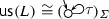
In the sequel, we will have to deal with cases where stability does not matter, and with cases where it matters and the LTSs in question are unstable. To exploit results on the latter when dealing with the former, we define a simple operator that, given an LTS, yields an unstable “$\cong _\mathsf {ft}$”-equivalent LTS. We let

The following lemma tells some properties of $\mathsf {us}(L)$.

Lemma 18

Assume A. For every L we have the following.

• 1. $\mathsf {us}(L)$ is unstable.

• 2. $\mathsf {us}(L) \cong _\mathsf {ft}L$.

• 3. If L is unstable, then $\mathsf {us}(L) \cong ^\mathsf {ft}_\mathsf {ft}L$ and $\mathsf {us}(L) \cong L$.

• 4. If there are $L_1$ and $L_2$ such that $L_1 \cong L_2$, $\varSigma _1 = \varSigma _2$, and $L_1 \ncong _\mathsf {ft}L_2$, then $\mathsf {us}(L) \cong L {\Vert }M_1^{\varSigma }$.

• 5. If there are $L_1$ and $L_2$ such that $L_1 \cong L_2$, $\varSigma _1 = \varSigma _2$, and $L_1 \ncong _\mathsf {tr}L_2$, then .

Proof

The first three claims are obvious.

For any L, $\mathsf {us}(L) \cong ^\mathsf {ft}_\mathsf {ft}L {\Vert }M_2^{\varSigma }$, because they both have $\varSigma$ as the alphabet, they are both unstable, and $M_2^{\varSigma }$ never blocks actions of L. With the assumptions of the fourth claim, Lemma 15 and the congruence property yield $L {\Vert }M_2^{\varSigma } \cong L {\Vert }M_1^{\varSigma }$. As a consequence, $\mathsf {us}(L) \cong L {\Vert }M_1^{\varSigma }$.

With the assumptions of the last claim, for any L, Lemma 14 yields . Clearly , because blocks all visible actions of L. Because “$\cong _\mathsf {ft}$” implies “$\cong _\mathsf {tr}$”, claim 4 yields $\mathsf {us}(L) \cong L {\Vert }M_1^{\varSigma }$. So . $\square$

The next lemma tells that if the congruence equates a stable and an unstable LTS, then stability does not matter at all.

Lemma 19

Assume that “$\cong ^\mathsf {ft}_\mathsf {ft}$” implies “$\cong$” and “$\cong$” is a congruence with respect to parallel composition and hiding. If there are a stable LTS $L_\mathsf {s}$ and an unstable LTS $L_\mathsf {u}$ such that $L_\mathsf {s} \cong L_\mathsf {u}$, then

• 1. , and

• 2. for any L, $L \cong \mathsf {us}(L)$.

Proof

Let $\varSigma := \varSigma (L_\mathsf {s}) \cup \varSigma (L_\mathsf {u})$ and . Clearly . The alphabet of $f(L_\mathsf {u})$ is , and by Lemma 2(1). Furthermore, $f(L_\mathsf {u})$ is obviously unstable. So . These yield . Therefore, .

Let L be any LTS. Clearly , so $L \cong \mathsf {us}(L)$. $\square$

The next lemma says that if the congruence does not preserve the alphabet, then, in the case of unstable LTSs, it throws away all information on traces and tree failures.

Lemma 20

Assume A. If “$\cong$” does not imply “$\cong _{\mathsf {\varSigma }}$”, then, for any L, .

Proof

Because “$\cong$” does not imply “$\cong _{\mathsf {\varSigma }}$”, there are $L_1$, $L_2$, and a such that $L_1 \cong L_2$, $a \in \varSigma _1$, and $a \notin \varSigma _2$. Let $\varSigma := (\varSigma _1 \cup \varSigma _2) {\setminus } \{a\}$.

If $L_1 \mathrel {{=}a{\Rightarrow }}$, then choose any $b \notin \{a, \tau , \varepsilon \}$ and let , where $\phi (b) := a$ and $\phi (x) := x$ if $x \ne b$. We have $f(L_1) \mathrel {{=}a{\Rightarrow }}$ but $\lnot (f(L_2) \mathrel {{=}a{\Rightarrow }})$. Although $a \notin \varSigma _2$, we have $\varSigma (f(L_2)) = \{a\}$ thanks to and $\phi$.

If $\lnot (L_1 \mathrel {{=}a{\Rightarrow }})$, then let . We have $\lnot (f(L_1) \mathrel {{=}a{\Rightarrow }})$ but $f(L_2) \mathrel {{=}a{\Rightarrow }}$.

In both cases, $f(L_1) \cong f(L_2)$, $\varSigma (f(L_1)) = \varSigma (f(L_2)) = \{a\}$, and $\mathsf {Tr}(f(L_1)) \ne \mathsf {Tr}(f(L_2))$. By Lemma 18(5), for any L, . $\square$

If $L_1 \cong L_2$ where $\cong$ is a congruence with respect to parallel composition, then , yielding $\mathsf {us}(L_1) \cong \mathsf {us}(L_2)$. Next we prove $\mathsf {us}(L_1) \cong \mathsf {us}(L_2)$ under five different assumptions, without assuming $L_1 \cong L_2$.

Lemma 21

Assume A. In each of the following situations we have $\mathsf {us}(L_1) \cong \mathsf {us}(L_2)$.

• 1. If $L_1 \cong _\mathsf {ft}L_2$.

• 2. If $L_1 \cong _\mathsf {tr}L_2$, and “$\cong$” implies “$\cong _{\mathsf {\varSigma }}$” but not “$\cong _\mathsf {ft}$”.

• 3. If $L_1 \cong _{\mathsf {\varSigma }}L_2$, and “$\cong$” implies “$\cong _{\mathsf {\varSigma }}$” but not “$\cong _\mathsf {tr}$”.

• 4. If $L_1 \cong ^{\textsf {}}_{\textsf {\#}} L_2$, and “$\cong$” does not imply “$\cong _{\mathsf {\varSigma }}$”.

• 5. If the alphabets of $L_1$ and $L_2$ are countable, and “$\cong$” does not imply “$\cong ^{\textsf {}}_{\textsf {\#}}$”.

Proof

1. By Lemma 18(2), $\mathsf {us}(L_1) \cong _\mathsf {ft}L_1 \cong _\mathsf {ft}L_2 \cong _\mathsf {ft}\mathsf {us}(L_2)$. So $\mathsf {us}(L_1) \cong _\mathsf {ft}\mathsf {us}(L_2)$. This implies $\mathsf {us}(L_1) \cong ^\mathsf {ft}_\mathsf {ft}\mathsf {us}(L_2)$, because $\mathsf {us}(L_1)$ and $\mathsf {us}(L_2)$ are unstable by Lemma 18(1). By assumption A, this implies $\mathsf {us}(L_1) \cong \mathsf {us}(L_2)$.

2. Let $L \in \{L_1, L_2\}$ and $f(L) := L {\Vert }M_1^{\varSigma }$. It is unstable because of $M_1^{\varSigma }$, so $f(L_1) \cong ^{\perp }_{\perp } f(L_2)$. We have $\varSigma (f(L)) = \varSigma$. Because $M_1^{\varSigma }$ may deadlock after any trace, Lemma 3 yields $\mathsf {Tf}(f(L)) = \{ (\sigma , K) \mid \sigma \in \mathsf {Tr}(L) \wedge K \subseteq \varSigma ^+ \}$. Because $L_1 \cong _\mathsf {tr}L_2$, we have $\varSigma _1 = \varSigma _2$ and $\mathsf {Tr}(L_1) = \mathsf {Tr}(L_2)$. These yield $f(L_1) \cong ^\mathsf {ft}_\mathsf {ft}f(L_2)$, implying $f(L_1) \cong f(L_2)$. The part of the condition after “and” justifies the use of Lemma 18(4), implying $\mathsf {us}(L_1) \cong f(L_1) \cong f(L_2) \cong \mathsf {us}(L_2)$.

3. The condition $L_1 \cong _{\mathsf {\varSigma }}L_2$ means that $\varSigma _1 = \varSigma _2$. By Lemma 18(5), .

4. The condition $L_1 \cong ^{\textsf {}}_{\textsf {\#}} L_2$ means that $\varSigma _1 \mathrel {\#}\varSigma _2$ is finite. Because “$\cong$” does not imply “$\cong _{\mathsf {\varSigma }}$”, there are $L'_1$, $L'_2$, and a such that $L'_1 \cong L'_2$, $a \in \varSigma '_1$, and $a \notin \varSigma '_2$. Let $\varSigma := (\varSigma '_1 \cup \varSigma '_2) {\setminus } \{a\}$. By Lemma 20, , where $\mathsf {us}(L'_2 {\setminus } \varSigma ) \cong \mathsf {us}(L'_1 {\setminus } \varSigma )$ follows from $L'_1 \cong L'_2$. Therefore, .

Choose any b such that $\tau \ne b \ne \varepsilon$. Let $\phi (a) := b$ and $\phi (x) := x$ when $x \ne a$. We have . So . Let $A = \{a_1, \ldots , a_n\}$ be any finite alphabet. For $0 \le i < n$, we have . By induction, .

If $\varSigma _1 \mathrel {\#}\varSigma _2$ is finite, then also $\varSigma _1 {\setminus } \varSigma _2$ and $\varSigma _2 {\setminus } \varSigma _1$ are finite. By Lemma 20, $.$

5. By the assumption, there are $L'_1$ and $L'_2$ such that $L'_1 \cong L'_2$ and $\varSigma '_1 \setminus \varSigma '_2$ is infinite. By Lemma 20, .

Let A be any countable alphabet. If $A = \emptyset$, then .

Otherwise there is $a \in A$. Because every infinite set contains a countably infinite subset, there is a bijection f from A to a subset of $\varSigma '_1 {\setminus } \varSigma '_2$. A surjection $\phi$ from $\varSigma '_1 {\setminus } \varSigma '_2$ to A is obtained by letting $\phi (x) := b$ if $x = f(b)$ and $\phi (x) := a$ if there is no b such that $x = f(b)$. We have .

So both $A = \emptyset$ and $A \ne \emptyset$ yield . We conclude . $\square$

We now have sufficient machinery to prove the main result. We deal first with the case where stability matters.

Lemma 22

Let x be any of $\mathsf {ft}$, $\mathsf {tr}$, and $\mathsf {en}$, and let $\mathsf {prev}(x)$ be the previous one (if $x \ne \mathsf {ft}$). Let y be any of $\mathsf {ft}$, $\mathsf {tr}$, , ${\#}$, and $\perp$, and let $\mathsf {prev}(y)$ be the previous one (if $y \ne \mathsf {ft}$). Assume A and that “$\cong$” implies “$\cong ^x_y$”. If $x \ne \mathsf {ft}$, assume also that “$\cong$” does not imply “$\cong ^{\mathsf {prev}(x)}_y$”. If $y \ne \mathsf {ft}$, assume also that “$\cong$” does not imply “$\cong ^x_{\mathsf {prev}(y)}$”. If $y = {\perp }$, assume also that the alphabets of the LTSs are countable. Then “$\cong$” is “$\cong ^x_y$”.

Proof

That “$\cong$” is “$\cong ^x_y$” means that “$\cong$” implies “$\cong ^x_y$” and “$\cong ^x_y$” implies “$\cong$”. The former was given in the assumption part of the lemma. Our task is to prove the latter for each x and y. So we assume that $L_1$ and $L_2$ are arbitrary LTSs such that $L_1 \cong ^x_y L_2$, and we have to prove that $L_1 \cong L_2$.

The definition of “$\cong ^x_y$” implies that $L_1$ and $L_2$ are both stable or both unstable.

If$L_1$and$L_2$are stable, then $L_1 \cong _x L_2$. There are three cases.

• If $x = \mathsf {ft}$, then $L_1$ and $L_2$ are stable and $L_1 \cong _\mathsf {ft}L_2$. By definition, $L_1 \cong ^\mathsf {ft}_\mathsf {ft}L_2$. It implies $L_1 \cong L_2$ by assumption A.

• If $x = \mathsf {tr}$, then $L_1 \cong _\mathsf {tr}L_2$ and there are $L'_1$ and $L'_2$ such that $L'_1 \cong L'_2$ but $L'_1 \ncong ^\mathsf {ft}_y L'_2$. Because $L'_1 \cong L'_2$ implies $L'_1 \cong ^\mathsf {tr}_y L'_2$, this means that $L'_1$ and $L'_2$ are both stable, $L'_1 \ncong _\mathsf {ft}L'_2$, and $\varSigma '_1 = \varSigma '_2$. Lemma 16 yields $L_1 \cong L_2$.

• If $x = \mathsf {en}$, then $L_1 \cong ^{\textsf {}}_{\textsf {en}} L_2$ and there are $L'_1$ and $L'_2$ such that $L'_1 \cong L'_2$ but $L'_1 \ncong ^\mathsf {tr}_y L'_2$. Because $L'_1 \cong L'_2$ implies $L'_1 \cong ^\mathsf {en}_y L'_2$, this means that $L'_1$ and $L'_2$ are both stable, $L'_1 \ncong _\mathsf {tr}L'_2$, and $\varSigma '_1 = \varSigma '_2$. Lemma 17 yields $L_1 \cong L_2$.

If$L_1$and$L_2$are unstable, then Lemma 18(3) yields $L_1 \cong \mathsf {us}(L_1)$ and $\mathsf {us}(L_2) \cong L_2$. We will soon show that the assumptions of Lemma 21 hold. By it, $\mathsf {us}(L_1) \cong \mathsf {us}(L_2)$, yielding $L_1 \cong L_2$.

Because $L_1$ and $L_2$ are unstable, $L_1 \cong ^x_y L_2$ implies $L_1 \cong _y L_2$. This gives the first condition of Lemma 21(1) to (4). The first condition of (5) is in the assumptions of the current lemma. When $y = \mathsf {tr}$ or , then “$\cong$” implies “$\cong ^x_y$” implies “$\cong _{\mathsf {\varSigma }}$”, because both “$\cong _x$” and “$\cong _y$” imply “$\cong _{\mathsf {\varSigma }}$”. This is needed by (2) and (3). When $y \ne \mathsf {ft}$, then there are $L'_1$ and $L'_2$ such that $L'_1 \cong L'_2$ yielding $L'_1 \cong ^x_y L'_2$, but $L'_1 \ncong ^x_{\mathsf {prev}(y)} L'_2$. They are unstable and satisfy $L'_1 \ncong _{\mathsf {prev}(y)} L'_2$. So “$\cong$” does not imply “$\cong _{\mathsf {prev}(y)}$”. This gives the last condition of (2) to (5) and completes the checking of the assumptions of Lemma 21. $\square$

Before continuing, it is perhaps a good idea to discuss a bit the fact that Lemma 22 refers to three equivalences that are grey in Fig. 1. First, in some cases “$\cong ^x_{\mathsf {prev}(y)}$” or “$\cong ^{\mathsf {prev}(x)}_y$” is grey. This is not a problem, because the lemma does not assume that it is a congruence. It only assumes that there are $L'_1$ and $L'_2$ such that $L'_1 \cong L'_2$ but $L'_1 \ncong ^x_{\mathsf {prev}(y)} L'_2$ and $L'_1 \ncong ^{\mathsf {prev}(x)}_y L'_2$.

Second, the lemma may claim that “$\cong$” is “$\cong ^x_y$” also when “$\cong ^x_y$” is grey. This is not a problem, because the lemma does not promise but assumes that “$\cong$” is a congruence. The lemma says that if there is a congruence with the assumed properties, then it is “$\cong ^x_y$”. If “$\cong ^x_y$” is not a congruence, then, with the chosen x and y, no congruences satisfy the assumptions of the lemma.

The case remains where stability does not matter.

Lemma 23

Let y be any of $\mathsf {ft}$, $\mathsf {tr}$, , ${\#}$, and $\perp$, and let $\mathsf {prev}(y)$ be the previous one (if $y \ne \mathsf {ft}$). Assume A and that “$\cong$” implies “$\cong _y$” but not “$\cong ^y_y$” or not “$\cong ^\mathsf {en}_y$”. If $y \ne \mathsf {ft}$, assume also that “$\cong$” does not imply “$\cong _{\mathsf {prev}(y)}$”. If $y = {\perp }$, assume also that the alphabets of the LTSs are countable. Then “$\cong$” is “$\cong _y$”.

Proof

We first show that there are $L''_1$ and $L''_2$ such that one of them is stable, the other is unstable, and $L''_1 \cong L''_2$. By the assumptions, there are $L'_1$ and $L'_2$ such that $L'_1 \cong L'_2$ and either $L'_1 \ncong ^y_y L'_2$ or $L'_1 \ncong ^\mathsf {en}_y L'_2$. Because “$\cong$” implies “$\cong _y$”, we have $L'_1 \cong _y L'_2$. If one of $L'_1$ and $L'_2$ is stable and the other is unstable, then they qualify as $L''_1$ and $L''_2$. Because $L'_1 \cong _y L'_2$, the only remaining possibility is that $L'_1$ and $L'_2$ are both stable and $L'_1 \ncong ^{\mathsf {}}_{\mathsf {en}} L'_2$. The latter implies $L'_1 \ncong ^{\mathsf {en}}_{\perp } L'_2$, so “$\cong$” does not imply “$\cong ^{\mathsf {en}}_{\perp }$” and Theorem 13 gives the claim.

As a consequence, for every L, Lemma 19(2) yields $L \cong \mathsf {us}(L)$. If $L_1 \cong _y L_2$, then $L_1 \cong \mathsf {us}(L_1) \cong \mathsf {us}(L_2) \cong L_2$ by Lemma 21 and the fact that “$\cong _\mathsf {tr}$” implies “$\cong _{\mathsf {\varSigma }}$”. Therefore, “$\cong _y$” implies “$\cong$”. It was assumed that “$\cong$” implies “$\cong _y$”. Hence “$\cong$” is “$\cong _y$”. $\square$

Theorem 24

Assume that “$\cong ^\mathsf {ft}_\mathsf {ft}$” implies “$\cong$” and “$\cong$” is a congruence with respect to parallel composition, hiding, and functional renaming. If “$\cong$” does not imply “$\cong ^{\textsf {}}_{\textsf {\#}}$”, then also assume that the alphabets of the LTSs are countable. Then “$\cong$” is one of the black equivalences in Fig. 1.

Proof

The congruence “$\cong$” implies at least “$\cong _{\perp }$”. Therefore, among the “$\cong _y$” where that it implies, there is a first one. For this y, if “$\cong$” does not imply the next black equivalence to the left of “$\cong _y$” in Fig. 1, then Lemma 23 applies, saying that “$\cong$” is “$\cong _y$”.

Otherwise, “$\cong$” implies some “$\cong ^x_y$” in Fig. 1. If “$\cong$” also implies the next equivalence to the left (if $x \ne \mathsf {ft}$) or the next equivalence above (if $y \ne \mathsf {ft}$), go there even if it is grey. Repeat this until it is possible to go neither left nor up. Now Lemma 22 applies, saying that “$\cong$” is “$\cong ^x_y$”.

As a consequence, the 20 equivalences in Fig. 1 contain all congruences that are implied by “$\cong ^\mathsf {ft}_\mathsf {ft}$” (making the countability assumption where needed). In Sect. 3 we proved that the black ones among them are congruences and the grey ones are not. $\square$

6 A somewhat general theory on adding stability preservation

Let “$\cong _o$” be a congruence that does not preserve initial stability. Here “o” stands for “original”. The goal is to find all congruences that are implied by “$\cong ^o_o$” (that is, “$\cong _o$” $\cap$ “$\cong ^{\perp }_{\perp }$”), in terms of the congruences that are implied by “$\cong _o$”. (There is no point in studying the case where “$\cong _o$” preserves initial stability, for then “$\cong ^o_o$” and “$\cong _o$” coincide.)

The first part of our work only needs very weak assumptions:

Assumption B. “$\cong _o$” and “$\cong$” are congruences with respect to parallel composition and hiding, “$\cong _o$” does not preserve initial stability, and “$\cong ^o_o$” implies “$\cong$”.

The following simple lemma will be used often.

Lemma 25

Assume B. If $L_1 \cong _oL_2$ and $L_1 \cong ^{\perp }_{\perp } L_2$, then $L_1 \cong L_2$.

Proof

The definitions of “$\cong ^o_o$” and “$\cong$” yield $L_1 \cong ^o_oL_2$ and $L_1 \cong L_2$. $\square$

We first deal with the case that also “$\cong$” does not preserve initial stability.

Lemma 26

If “$\cong$” is a congruence with respect to “${\Vert }$” and “${\setminus }$” and does not preserve initial stability, then there is an unstable LTS U such that .

Proof

By the assumption, there are a stable LTS $L_\mathsf {s}$ and an unstable LTS $L_\mathsf {u}$ such that $L_\mathsf {s} \cong L_\mathsf {u}$. Let $\varSigma = \varSigma (L_\mathsf {s})$. We have , so . The latter is unstable. $\square$

Theorem 27

Assume B. If “$\cong$” does not preserve initial stability, then “$\cong _o$” implies “$\cong$”.

Proof

Assume that $L_1 \cong _oL_2$. We have to show $L_1 \cong L_2$.

Let U be like in Lemma 26. Because “$\cong _o$” is a congruence, we have $L_1 {\Vert }U \cong _oL_2 {\Vert }U$. Both $L_1 {\Vert }U$ and $L_2 {\Vert }U$ are unstable because U is unstable. Therefore, Lemma 25 yields $L_1 {\Vert }U \cong L_2 {\Vert }U$.

Because “$\cong$” is a congruence, and similarly $L_2 \cong L_2 {\Vert }U$. Altogether $L_1 \cong L_1 {\Vert }U \cong L_2 {\Vert }U \cong L_2$ giving $L_1 \cong L_2$. $\square$

In the rest of this section “$\cong$” does preserve initial stability. Therefore, “$\cong$” can be represented in the form “$\cong ^x_y$”, where “$\cong _x$” is a binary relation such that for stable LTSs $L_1 \cong _x L_2 \Leftrightarrow L_1 \cong L_2$, and “$\cong _y$” is a binary relation such that for unstable LTSs $L_1 \cong _y L_2 \Leftrightarrow L_1 \cong L_2$. We now show that for every “$\cong$”, “$\cong _y$” can be chosen so that it is a congruence that is implied by “$\cong _o$”.

Application of Lemma 26 to “$\cong _o$” in place of “$\cong$” tells that there is an unstable $U_o$ such that . We define $L_1 \cong _\tau L_2 :\Leftrightarrow L_1 {\Vert }U_o \cong L_2 {\Vert }U_o$, and prove that “$\cong _\tau$” qualifies as “$\cong _y$”.

Lemma 28

Assume B. Then “$\cong _\tau$” is a congruence.

Proof

Because “$\cong$” is an equivalence, Lemma 6 implies that “$\cong _\tau$” is an equivalence as well. Let $\mathsf {op}(L)$ be any operator with respect to which “$\cong$” is a congruence. We assume that $L_1 \cong _\tau L_2$ and show that $\mathsf {op}(L_1) \cong _\tau \mathsf {op}(L_2)$.

By the definition, $L_1 {\Vert }U_o \cong L_2 {\Vert }U_o$. Because “$\cong$” is a congruence, we have $\mathsf {op}(L_1 {\Vert }U_o) \cong \mathsf {op}(L_2 {\Vert }U_o)$ and $\mathsf {op}(L_1 {\Vert }U_o) {\Vert }U_o \cong \mathsf {op}(L_2 {\Vert }U_o) {\Vert }U_o$.

Let $L \in \{L_1, L_2\}$. Because and “$\cong _o$” is a congruence, we have and $\mathsf {op}(L) {\Vert }U_o \cong _o\mathsf {op}(L {\Vert }U_o) {\Vert }U_o$. Both $\mathsf {op}(L) {\Vert }U_o$ and $\mathsf {op}(L {\Vert }U_o) {\Vert }U_o$ are unstable, so Lemma 25 yields $\mathsf {op}(L) {\Vert }U_o \cong \mathsf {op}(L {\Vert }U_o) {\Vert }U_o$.

We have $\mathsf {op}(L_1) {\Vert }U_o \cong \mathsf {op}(L_1 {\Vert }U_o) {\Vert }U_o \cong \mathsf {op}(L_2 {\Vert }U_o) {\Vert }U_o \cong \mathsf {op}(L_2) {\Vert }U_o$. Therefore, $\mathsf {op}(L_1) \cong _\tau \mathsf {op}(L_2)$. $\square$

Lemma 29

Assume B. Then “$\cong _o$” implies “$\cong _\tau$”.

Proof

Assume that $L_1 \cong _oL_2$. Because “$\cong _o$” is a congruence, we have $L_1 {\Vert }U_o \cong _oL_2 {\Vert }U_o$. Since $L_1 {\Vert }U_o$ and $L_2 {\Vert }U_o$ are unstable, Lemma 25 yields $L_1 {\Vert }U_o \cong L_2 {\Vert }U_o$, that is, $L_1 \cong _\tau L_2$. $\square$

Lemma 30

Assume B and that $L_1$ and $L_2$ are unstable. Then $L_1 \cong L_2$ if and only if $L_1 \cong _\tau L_2$.

Proof

Assume that $L_1 \cong L_2$. Because “$\cong$” is a congruence, we have $L_1 {\Vert }U_o \cong L_2 {\Vert }U_o$, that is, $L_1 \cong _\tau L_2$.

Assume that $L_1 \cong _\tau L_2$. That is, $L_1 {\Vert }U_o \cong L_2 {\Vert }U_o$. Like above, we have . Because $L_1$ and $L_1 {\Vert }U_o$ are unstable, Lemma 25 yields $L_1 \cong L_1 {\Vert }U_o$. Similar reasoning yields $L_2 \cong L_2 {\Vert }U_o$. Altogether $L_1 \cong L_1 {\Vert }U_o \cong L_2 {\Vert }U_o \cong L_2$. $\square$

Theorem 31

Assume B. If “$\cong$” preserves initial stability, then “$\cong$” can be represented as “$\cong ^x_y$” for some “$\cong _x$” and “$\cong _y$” such that “$\cong _y$” is a congruence that is implied by “$\cong _o$”.

Proof

“$\cong _y$” is “$\cong _\tau$”. $\square$

The fact that “” is a congruence tells that a corresponding theorem for “$\cong _x$” must be more complicated. This is because the congruence “” is implied by “$\cong ^{\textsf {tr}}_{\textsf {tr}}$”, but no congruence implied by “$\cong _\mathsf {tr}$” matches “” on stable LTSs. Therefore, in the place of “$\cong _x$” we will use a relation that checks that $L_1 \cong ^{\textsf {}}_{\textsf {en}} L_2$ and, roughly speaking, for each $a \in \mathsf {en}(L_1)$, the behaviours of $L_1$ after a and $L_2$ after a are in a congruence that is implied by “$\cong _o$”. Our proof relies on much stronger assumptions than assumption B. The first part of the assumptions is shown below, and the second part will be presented after we have developed the necessary notions.

Assumption C. “$\cong _o$” and “$\cong$” are congruences with respect to parallel composition, hiding, relational renaming, and action prefix; “$\cong _o$” does not but “$\cong$” does preserve initial stability; and “$\cong ^o_o$” implies “$\cong$”.

We now define the congruence that is implied by “$\cong _o$”.

Definition 32

For any LTSs $L_1$ and $L_2$, we define $L_1 \cong ^\bullet L_2$ if and only if there is $x \notin \varSigma _1 \cup \varSigma _2 \cup \{\tau , \varepsilon \}$ such that $x.L_1 \cong x.L_2$.

Lemma 33

Assume C. If $L_1 \cong ^\bullet L_2$, then $a.L_1 \cong a.L_2$ holds for all $a \notin \{\tau , \varepsilon \}$.

Proof

Let x be like in Definition 32. Because “$\cong$” is a congruence with respect to “$\varPhi$”, $x.L_1 \cong x.L_2$ implies $(x.L_1)\{(x,a)\} \cong (x.L_2)\{(x,a)\}$. Because $x \notin \varSigma _1 \cup \varSigma _2$ we have $a.L_1 = (x.L_1)\{(x,a)\} \cong (x.L_2)\{(x,a)\} = a.L_2$, yielding $a.L_1 \cong a.L_2$. $\square$

Lemma 34

Assume C. The relation “$\cong ^\bullet$” is a congruence with respect to “${\Vert }$”, “${\setminus }$”, “$\varPhi$”, and “a.”.

Proof

Let $L_1$, $L_2$ and $L_3$ be LTSs, a a visible action, A a set of visible actions, and $\varPhi$ a set of pairs of visible actions. Let x be a visible action that is not in $A \cup \{a\} \cup \varSigma _1 \cup \varSigma _2 \cup \varSigma _3$ and not in any pair of $\varPhi$. By Lemma 33, whenever $L \cong ^\bullet L'$ holds below for some L and $L'$, we have $x.L \cong x.L'$.

Because “$\cong$” is an equivalence, we have the following. Obviously $x.L_1 \cong x.L_1$. So “$\cong ^\bullet$” is reflexive. If $L_1 \cong ^\bullet L_2$, then $x.L_1 \cong x.L_2$. So $x.L_2 \cong x.L_1$ and $L_2 \cong ^\bullet L_1$. Thus “$\cong ^\bullet$” is symmetric. If $L_1 \cong ^\bullet L_2$ and $L_2 \cong ^\bullet L_3$, then $x.L_1 \cong x.L_2$ and $x.L_2 \cong x.L_3$, so $x.L_1 \cong x.L_3$. Therefore, $L_1 \cong ^\bullet L_3$ and “$\cong ^\bullet$” is transitive.

Because $x \notin \varSigma _1 \cup \varSigma _2 \cup \varSigma _3 \cup \{\tau , \varepsilon \}$, we have $x.(L_i {\Vert }L_3) \equiv (x.L_i) {\Vert }(x.L_3)$ when $i=1$ or $i=2$. If $L_1 \cong ^\bullet L_2$, then $x.L_1 \cong x.L_2$. Because “$\cong$” is a congruence with respect to “${\Vert }$”, we have $(x.L_1) {\Vert }(x.L_3) \cong (x.L_2) {\Vert }(x.L_3)$. So $x.(L_1 {\Vert }L_3) \cong x.(L_2 {\Vert }L_3)$ and $L_1 {\Vert }L_3 \cong ^\bullet L_2 {\Vert }L_3$. Similar reasoning proves $L_3 {\Vert }L_1 \cong ^\bullet L_3 {\Vert }L_2$. Therefore, “$\cong ^\bullet$” is a congruence with respect to “${\Vert }$”.

Because $x \notin A$, we have $x.(L_i {\setminus } A) \equiv (x.L_i) {\setminus } A$ when $i=1$ or $i=2$. If $L_1 \cong ^\bullet L_2$, then $x.L_1 \cong x.L_2$. Because “$\cong$” is a congruence with respect to “${\setminus }$”, we have $(x.L_1) {\setminus } A \cong (x.L_2) {\setminus } A$. So $x.(L_1 {\setminus } A) \cong x.(L_2 {\setminus } A)$ and $L_1 {\setminus } A \cong ^\bullet L_2 {\setminus } A$. Therefore, “$\cong ^\bullet$” is a congruence with respect to “${\setminus }$”.

By the choice of x, we have $x.(L_i\varPhi ) \equiv (x.L_i)\varPhi$ when $i=1$ or $i=2$. If $L_1 \cong ^\bullet L_2$, then $x.L_1 \cong x.L_2$. Because “$\cong$” is a congruence with respect to “$\varPhi$”, we have $(x.L_1)\varPhi \cong (x.L_2)\varPhi$. So $x.(L_1\varPhi ) \cong x.(L_2\varPhi )$ and $L_1\varPhi \cong ^\bullet L_2\varPhi$. Therefore, “$\cong ^\bullet$” is a congruence with respect to “$\varPhi$”.

If $L_1 \cong ^\bullet L_2$, then $a.L_1 \cong a.L_2$ by Lemma 33. Because “$\cong$” is a congruence with respect to “x.”, we have $x.(a.L_1) \cong x.(a.L_2)$. So $a.L_1 \cong ^\bullet a.L_2$. Therefore, “$\cong ^\bullet$” is a congruence with respect to “a.”. By choosing a so that it is not in $\varSigma _1 \cup \varSigma _2$ we also get $\tau .L_1 = (a.L_1) {\setminus } \{a\} \cong ^\bullet (a.L_2) {\setminus } \{a\} = \tau .L_2$, because we have already shown that “$\cong ^\bullet$” is a congruence with respect to “${\setminus }$”. Thus “$\cong ^\bullet$” is a congruence with respect to “$\tau .$”. $\square$

Lemma 35

Assume C. Then “$\cong _o$” implies “$\cong ^\bullet$”.

Proof

Assume that $L_1 \cong _oL_2$. Let $x \notin \varSigma _1 \cup \varSigma _2 \cup \{\tau , \varepsilon \}$. By the congruence property, we have $x.L_1 \cong _ox.L_2$. Since $x.L_1$ and $x.L_2$ are stable, Lemma 25 yields $x.L_1 \cong x.L_2$. That is, $L_1 \cong ^\bullet L_2$. $\square$

We will soon make it precise what we mean by the behaviour of a stable LTS after a visible action. As a preparatory step, let $\varSigma$ be a set of visible actions and x a visible action. We define as the two-state LTS whose alphabet is $\varSigma \cup \{x\}$ and transitions are $\{({\hat{s}}_x, x, s_x)\} \cup \{ (s_x, a, s_x) \mid a \in \varSigma \}$.

Let $L = (S, \varSigma , \varDelta , {\hat{s}})$ be a stable LTS, $a \in \varSigma$, and $x \notin \varSigma \cup \{\tau , \varepsilon \}$. We will soon use the LTS . To get intuition for it, we now show that it is isomorphic to the reachable part of $L' = (S', \varSigma ', \varDelta ', {\hat{s}}')$, where ${\hat{s}}'$ is a new state (that is, ${\hat{s}}' \notin S$), $S' = S \cup \{{\hat{s}}'\}$, $\varSigma ' = \varSigma \cup \{x\}$, and $\varDelta ' = \varDelta \cup \{ ({\hat{s}}', x, s) \mid ({\hat{s}}, a, s) \in \varDelta \}$ (Fig. 5).

The LTS has two states ${\hat{s}}_x$ and $s_x$. The states of $L^a_x$ are of the form $(s,s')$, where $s \in S$ and $s' \in \{{\hat{s}}_x, s_x\}$. Because the alphabet of both $L\{(a,x)(a,a)\}$ and is $\varSigma \cup \{x\}$, and because has no $\tau$-transitions, the transitions of $L^a_x$ are of three forms: $(s, {\hat{s}}_x) \mathrel {{-}x{\rightarrow }} (s', s_x)$ where (thanks to the renaming) $(s,a,s') \in \varDelta$; $(s, s_x) \mathrel {{-}b{\rightarrow }} (s', s_x)$ where $b \in \varSigma$ and $(s,b,s') \in \varDelta$; and $(s, s'_x) \mathrel {{-}\tau {\rightarrow }} (s', s'_x)$ where $(s,\tau ,s') \in \varDelta$ and $s'_x \in \{{\hat{s}}_x, s_x\}$. Once ${\hat{s}}_x$ has been left, it cannot be re-entered. Furthermore, L is stable. Therefore, the states of the form $(s, {\hat{s}}_x)$ where $s \ne {\hat{s}}$ are unreachable. The states of the form $(s, s_x)$ and their outgoing transitions constitute a copy of the reachable part of L, in addition to which there is the transition $({\hat{s}}, {\hat{s}}_x) \mathrel {{-}x{\rightarrow }} (s, s_x)$ for every $({\hat{s}}, a, s)$ of the reachable part of L.

The LTS $L^a_x {\setminus } \{x\}$ is otherwise similar, but it lacks x in its alphabet and its initial transitions are labelled with $\tau$ instead of x. It is independent of the choice of x (as long as $x \notin \varSigma \cup \{\tau , \varepsilon \}$). In structural operational semantics,

$$\begin{aligned} \frac{L \mathrel {{-}a{\rightarrow }} L'}{L^a_x {\setminus } \{x\} \mathrel {{-}\tau {\rightarrow }} L'} \end{aligned}$$

and that is all $L^a_x {\setminus } \{x\}$ can do. From now on we denote it with $a^{-1}L$. That is, if L is a stable LTS, $a \in \varSigma$, and $x \notin \varSigma \cup \{\tau , \varepsilon \}$, then we define

It is easy to check that $\varSigma (a^{-1}L) = \varSigma$.

Lemma 36

Assume C. If $L_1 \cong L_2$ where $L_1$ and $L_2$ are stable, then $\varSigma _1 = \varSigma _2$, $\mathsf {en}(L_1) = \mathsf {en}(L_2)$, and $a^{-1}L_1 \cong ^\bullet a^{-1}L_2$ for every $a \in \mathsf {en}(L_1)$.

Proof

Theorem 13 yields $L_1 \cong ^{\textsf {}}_{\textsf {en}} L_2$, that is, $\varSigma _1 = \varSigma _2$ and $\mathsf {en}(L_1) = \mathsf {en}(L_2)$. The congruence properties of “$\cong$” and the definition of $a^{-1}L$ yield $x.(a^{-1}L_1) \cong x.(a^{-1}L_2)$, from which the definition of “$\cong ^\bullet$” yields the last claim. $\square$

To prove the converse of Lemma 36, we discuss the construction of L, when $a^{-1}L$ is given for each $a \in \mathsf {en}(L)$. Then we present the assumptions we will use in addition to assumption C.

Fig. 5

Illustrating $L^a_x$ (left), $a^{-1}L$, and $idf (L)$ (right)

Let A be a set of visible actions and $L_a$ be an LTS for each $a \in A$. If A is finite, then it is of the form $\{a_1, \ldots , a_n\}$, where the $a_i$ are distinct from each other. We define finite deterministic choice between $a_1.L_{a_1}$, ..., $a_n.L_{a_n}$ as $\sum _{a \in A} a.L_a = a_1.L_{a_1} + \cdots + a_n.L_{a_n}$. Infinite deterministic choice is the natural extension to infinite A, and deterministic choice is finite or infinite deterministic choice. “Deterministic” signifies that $\sum _{a \in A} a.L_a$ has precisely one initial transition for each $a \in A$, and no other initial transitions.

Definition 37

If L is stable, then by its initially deterministic form we mean

$$\begin{aligned} idf (L) \ =\ \sum _{a \in \mathsf {en}(L)} a.(a^{-1}L)\ \text {.} \end{aligned}$$

Assumption D. $L \cong _o idf (L)$ holds for every stable L, and “$\cong$” is a congruence with respect to infinite deterministic choice.

We need not assume that “$\cong$” is a congruence with respect to finite deterministic choice, because Lemma 40 will tell that it is. However, we first focus on the big picture, and present the result where Assumption D is needed.

Lemma 38

Assume C and D. If $L_1$ and $L_2$ are stable, $\mathsf {en}(L_1) = \mathsf {en}(L_2)$, and $a^{-1}L_1 \cong ^\bullet a^{-1}L_2$ for every $a \in \mathsf {en}(L_1)$, then $L_1 \cong L_2$.

Proof

Clearly $idf (L)$ is stable, so Assumption D and Lemma 25 imply $L_1 \cong idf (L_1)$ and $idf (L_2) \cong L_2$. Because $a^{-1}L_1 \cong ^\bullet a^{-1}L_2$ and a is visible, by Lemma 33, $a.(a^{-1}L_1)$$\cong$$a.(a^{-1}L_2)$ for each $a \in \mathsf {en}(L_1) = \mathsf {en}(L_2)$. Thus Lemma 40 (in the finite case) and Assumption D (in the infinite case) yield $idf (L_1) \cong idf (L_2)$. $\square$

We can now prove a result that resembles Lemma 30 and can be used to characterize the “$\cong _x$” in Theorem 31.

Theorem 39

Let “congruence” mean with respect to “${\Vert }$”, “${\setminus }$”, “$\varPhi$”, and “a.”. Let “$\cong _o$” and “$\cong$” be congruences such that “$\cong ^o_o$” implies “$\cong$”, and “$\cong _o$” does not but “$\cong$” does preserve initial stability. Also assume D. There is a congruence “$\cong ^\bullet$” implied by “$\cong _o$” such that for stable LTSs, $L_1 \cong L_2$ if and only if $\varSigma _1 = \varSigma _2$, $\mathsf {en}(L_1) = \mathsf {en}(L_2)$, and $a^{-1} L_1 \cong ^\bullet a^{-1} L_2$ for every $a \in \mathsf {en}(L_1)$.

Proof

The assumptions in the theorem imply Assumption C. By Lemmas 34 and 35, the relation in Definition 32 is a congruence implied by “$\cong _o$”. Lemmas 36 and 38 give the last claim. $\square$

The use of Assumption D reduces the generality of this theorem. The rest of this section is devoted to a brief analysis on conditions where Assumption D holds. Based on it, we will see in the next section that the first half of Assumption D is not a problem with CFFD equivalence.

Next we show that if we restrict ourselves to LTSs L such that $\mathsf {en}(L)$ is finite whenever L is stable, then the latter part of D need not be assumed. We do that by showing that the choice operator can be constructed from parallel composition and functional renaming, if the LTSs are stable. If A and B are sets of visible actions, we define , where each thick arrow denotes a transition for each member of the label of the arrow.

Lemma 40

If $L_1$ and $L_2$ are stable, then

$$\begin{aligned} L_1 + L_2 \ \equiv \ \lfloor \,\lceil L_1\rceil ^{[1]} \,{\Vert }\, \lceil L_2\rceil ^{[2]} \,{\Vert }\, C(\varSigma _1^{[1]}, \varSigma _2^{[2]})\,\rfloor _{[1,2]}\ \text {.} \end{aligned}$$

Proof

Let the right hand side be called R. Because of the renaming, the alphabets of $\lceil L_1\rceil ^{[1]}$ and $\lceil L_2\rceil ^{[2]}$ are disjoint and the alphabet of $C(\ldots )$ is their union. So all visible transitions of R are either joint transitions by $\lceil L_1\rceil ^{[1]}$ and $C(\ldots )$ or joint transitions by $\lceil L_2\rceil ^{[2]}$ and $C(\ldots )$. Thanks to $\lfloor \ldots \rfloor _{[1,2]}$, they have the labels that are used in $L_1$ and $L_2$. Because $C(\ldots )$ has no $\tau$-transitions, all $\tau$-transitions of R arise from $\tau$-transitions of $L_1$ or $\tau$-transitions of $L_2$.

Let the states of $C(\ldots )$ be called $c_1$, ${\hat{c}}$, and $c_2$. The initial state of R is $({\hat{s}}_1, {\hat{s}}_2, {\hat{c}})$. It has no $\tau$-transitions, because $L_1$ and $L_2$ are stable. It has the transitions $({\hat{s}}_1, {\hat{s}}_2, {\hat{c}}) \mathrel {{-}a{\rightarrow }} (s_1, {\hat{s}}_2, c_1)$ where ${\hat{s}}_1 \mathrel {{-}a{\rightarrow }} s_1$ is a transition of $L_1$, and $({\hat{s}}_1, {\hat{s}}_2, {\hat{c}}) \mathrel {{-}a{\rightarrow }} ({\hat{s}}_1, s_2, c_2)$ where ${\hat{s}}_2 \mathrel {{-}a{\rightarrow }} s_2$ is a transition of $L_2$. When in $c_1$, $C(\ldots )$ stays there forever, blocks $L_2$ in ${\hat{s}}_2$, and lets $L_1$ proceed freely. Therefore, states of the form $(s_1, {\hat{s}}_2, c_1)$ and their outgoing transitions constitute a copy of $L_1$. A similar claim holds about $({\hat{s}}_1, s_2, c_2)$ and $L_2$. $\square$

This construction does not generalize to infinite choice, because infinite parallel composition is a problematic thing. For instance, if , then $a \in \mathsf {Tr}(L {\Vert }L {\Vert }\cdots )$, but if , then $a \notin \mathsf {Tr}(L {\Vert }L {\Vert }\cdots )$, because an infinite number of $\tau$-transitions would be needed to enable a. This example warns that we cannot take extensions of the congruence property to infinite operators for granted. In Fig. 1, “$\cong ^{\textsf {en}}_{\textsf {\#}}$” is a congruence with respect to finite but not with respect to infinite (nondeterministic!) choice, because of the counter-example where and for $i \in {\mathbb {N}}$. The author has found neither a proof nor a counter-example to $idf (L_1) \cong idf (L_2)$ when $L_1$ and $L_2$ are stable, $\varSigma _1 = \varSigma _2$, $\mathsf {en}(L_1) = \mathsf {en}(L_2)$ is infinite, $a^{-1}L_1 \cong a^{-1}L_2$ for each $a \in \mathsf {en}(L_1)$, C is assumed, and D is not.

A relation that satisfies assumption C (and, by Lemma 40, is thus a congruence with respect to finite choice) but is not a congruence with respect to deterministic infinite choice, would be an oddity. So the inability of our theory to deal with such relations without an extra assumption is perhaps not a big drawback. The first part of Assumption D is, however, significant. It says that if L is stable, then $L \cong _o idf (L)$. For instance, Milner’s observation equivalence does not satisfy it.

The only difference between a stable L and $idf (L)$ is that the choice between initial transitions with the same label is postponed to a choice between $\tau$-transitions after the initial transition (see Fig. 5). This is formalized next.

Lemma 41

If L is a stable LTS, then $idf (L) \equiv (S', \varSigma , \varDelta ', {\hat{s}}')$, where $S' = S$$\cup$$\{{\hat{s}}'\}$$\cup$$\{s_a \mid a \in \mathsf {en}(L)\}$, the added states are distinct from each other and the states in S, and $\varDelta '$ is obtained from $\varDelta$ by adding, for each $a \in \mathsf {en}(L)$, the transition ${\hat{s}}' \mathrel {{-}a{\rightarrow }} s_a$ and for each $({\hat{s}}, a, s) \in \varDelta$ the transitions $s_a \mathrel {{-}\tau {\rightarrow }} s$.

Proof

For each $a \in \mathsf {en}(L)$, $a^{-1}L$ and $a.(a^{-1}L)$ have the same alphabet as L, and thus also $idf (L)$ has the same alphabet. The LTS characterization $L^{a}_x {\setminus } \{x\}$ of $a^{-1}L$ picks the part of L that starts with a-transitions, and hides the initial a-transitions. The construction of $idf (L)$ adds an a-transition to the front of $a^{-1}L$ and puts the resulting $a.(a^{-1}L)$ together. $\square$

7 Application to CFFD equivalence

In this section we apply the theory in the previous section to prove that the stability-preserving CFFD equivalence implies precisely 79 congruences. Throughout this section the word “congruence” means congruence with respect to parallel composition, hiding, relational renaming, action prefix, and infinite deterministic choice. To keep this section reasonably short, we skip some proofs that consist of routine checking, and also skip the definitions that are only needed in such proofs. The definitions can be found in [17].

The state $s_0$diverges, denoted with $s_0 \mathrel {{-}\tau ^\omega {\rightarrow }}$, if and only if there are states $s_i$ for every $i > 0$ such that $s_0 \mathrel {{-}\tau {\rightarrow }} s_1 \mathrel {{-}\tau {\rightarrow }} \ldots$. The set of divergence traces of L is $\mathsf {Div}(L) = \{ \sigma \in \varSigma ^* \mid \exists s: {\hat{s}} \mathrel {{=}\sigma {\Rightarrow }} s \mathrel {{-}\tau ^\omega {\rightarrow }} \}$. The notation $s \mathrel {{=}\sigma {\Rightarrow }}$ extends naturally to infinite sequences of visible actions. The set of infinite traces of L is $\mathsf {Inf}(L) = \{ \xi \in \varSigma ^\omega \mid {\hat{s}} \mathrel {{=}\xi {\Rightarrow }} \}$. If ${\hat{s}} \mathrel {{-}a_1{\rightarrow }} s_1 \mathrel {{-}a_2{\rightarrow }} \ldots$ is an infinite path of L, then the projection of $a_1 a_2 \cdots$ on visible actions is either a divergence trace (if it is finite) or an infinite trace (if it is infinite).

The set of stable failures of L is $\mathsf {Sf}(L) = \{ (\sigma , A) \in \varSigma ^* \times 2^\varSigma \mid \exists s: {\hat{s}} \mathrel {{=}\sigma {\Rightarrow }} s$$\wedge$$\forall a \in A \cup \{\tau \}: \lnot (s \mathrel {{-}a{\rightarrow }}) \}$. That is, a stable failure is a pair consisting of a trace and a set of visible actions such that L can execute the trace and then be in a stable state where it cannot execute any element of the set. Assume that ${\hat{s}} \mathrel {{=}\sigma {\Rightarrow }} s$. If a stable state can be reached from s via $\tau$-transitions, then $(\sigma , \emptyset )$ is a stable failure of L, and otherwise $\sigma$ is a divergence trace of L. Therefore, $\mathsf {Tr}(L) = \mathsf {Div}(L) \cup \{ \sigma \mid (\sigma , \emptyset ) \in \mathsf {Sf}(L) \}$.

The LTSs $L_1$ and $L_2$ are CFFD-equivalent, that is, $L_1 \cong _\mathsf {CFFD}L_2$, if and only if $\varSigma _1 = \varSigma _2$, $\mathsf {Sf}(L_1) = \mathsf {Sf}(L_2)$, $\mathsf {Div}(L_1) = \mathsf {Div}(L_2)$, and $\mathsf {Inf}(L_1) = \mathsf {Inf}(L_2)$.

It is obvious from the definition and Lemma 41 that if L is a stable LTS, then $L \cong _\mathsf {CFFD} idf (L)$. That is, the first part of Assumption D holds for CFFD equivalence. It is also clear that $L \cong _\mathsf {CFFD}\tau .L$ for any LTS L.

Fig. 6

All congruences with respect to a.L, $L {\setminus } A$, $L\varPhi$, and $L {\Vert }L'$ that are implied by CFFD equivalence. There is a path from “$\cong _1$” down to “$\cong _2$” if and only if “$\cong _1$” implies “$\cong _2$”. Each congruence preserves all sets listed along the paths from it down to “$\cong _{\perp }$”. However, the definition of a congruence need not mention those sets that can be determined from the sets that are mentioned [17]

CFFD equivalence implies precisely 40 congruences with respect to parallel composition, hiding, relational renaming and action prefix. They are shown in Fig. 6 [17]. The figure shows “$\cong _{\perp }$”, “$\cong _{\mathsf {\varSigma }}$” and “$\cong _\mathsf {tr}$” but not “$\cong ^{\textsf {}}_{\textsf {\#}}$”, because it is not a congruence with respect to relational renaming. The figure also shows the CSP failures divergences equivalence [15]. For convenience, we call other congruences in the figure than “$\cong _{\perp }$” and “$\cong _{\mathsf {\varSigma }}$” black, and “$\cong _{\mathsf {\varSigma }}$” is grey.

The congruences use two kinds of traces, two kinds of divergence traces, four kinds of infinite traces, and five kinds of failures. For instance, $\mathsf {anT}(L)$ and $\mathsf {anI}(L)$ are the traces and infinite traces whose prefixes are not divergence traces; $\mathsf {minD}(L)$ is the divergence traces whose proper prefixes are in $\mathsf {anT}(L)$; $\mathsf {anF}(L)$ is the stable failures whose trace part is in $\mathsf {anT}(L)$; and $\mathsf {sanF}(L)$ is the same with the additional requirement that if $(\sigma , \{a\}) \in \mathsf {sanF}(L)$, then $\sigma a \notin \mathsf {Div}(L)$. The CSP failures divergences equivalence results from requiring that $\varSigma _1 = \varSigma _2$, $\mathsf {anF}(L_1) = \mathsf {anF}(L_2)$, $\mathsf {minD}(L_1) = \mathsf {minD}(L_2)$, and $\mathsf {anI}(L_1) = \mathsf {anI}(L_2)$. When this holds, then also $\mathsf {anT}(L_1) = \mathsf {anT}(L_2)$ and $\mathsf {sanF}(L_1) = \mathsf {sanF}(L_2)$. The set $\mathsf {anI}$ is needed here although it is typically not used with CSP, beacuse there something is assumed to the effect that the LTSs are finitely branching, which we do not assume.

Lemma 42

If L is stable, then $\mathsf {en}(L) = \mathsf {Tr}(L) \cap \varSigma = \{a \in \varSigma \mid (\varepsilon , \{a\}) \notin \mathsf {Sf}(L)\} = (\mathsf {minD}(L) \cup \mathsf {anT}(L)) \cap \varSigma$.

Proof

Because $\lnot ({\hat{s}} \mathrel {{-}\tau {\rightarrow }})$, we have $\mathsf {Tr}(L) \cap \varSigma = \{ a \in \varSigma \mid {\hat{s}} \mathrel {{-}a{\rightarrow }} \} = \mathsf {en}(L)$. For the same reason, only ${\hat{s}}$ can introduce stable failures of the form $(\varepsilon , A)$. Furthermore, $\varepsilon \notin \mathsf {minD}(L)$ because $\lnot ({\hat{s}} \mathrel {{-}\tau {\rightarrow }})$. Therefore, each $a \in \mathsf {Tr}(L) \cap \varSigma$ is either a minimal divergence trace or an always nondivergent trace. $\square$

We mention without proof that these 40 congruences are also congruences with respect to choice between stable LTSs, and thus with respect to infinite deterministic choice. Intuitively, this is because $\mathsf {Tr}(\sum L_i) = \bigcup \mathsf {Tr}(L_i)$; similarly with $\mathsf {Div}$ and $\mathsf {Inf}$; $\mathsf {minD}$ has a similar formula where only the minimal elements of the union are kept; $\mathsf {anT}$, $\mathsf {anI}$, $\mathsf {eanI}$, and $\mathsf {aenI}$ have similar formulas with (minimal) divergence traces used to fix the result; the failures of any kind of the form $(\varepsilon , A)$ are dealt with similarly to Lemma 42; and the failures $(\sigma , A)$ with $\sigma \ne \varepsilon$ have somewhat similar formulas as $\mathsf {anT}$.

Furthermore, if “$\cong _x$” is any of the black congruences, then “$\cong ^x_x$” is a congruence, because by Lemma 42 it is the intersection of “$\cong _x$” and “”. Because it preserves initial stability, it is possible to reason the stable failures of the form $(\varepsilon , A)$ of the result of the choice between any LTSs from the stable failures of the component LTSs. Thus “$\cong ^x_x$” is a congruence also with respect to both finite and infinite choice between any LTSs (stable and unstable).

By Theorem 27, the congruences implied by “$\cong ^\mathsf {CFFD}_\mathsf {CFFD}$” that do not preserve initial stability are precisely the 40 congruences in Fig. 6. This result does not assume the congruence property with respect to infinite deterministic choice.

We now turn our attention to congruences that preserve initial stability. By Theorem 31, they can be represented in the form “$\cong ^x_y$”, where “$\cong _y$” can only be one of the 39 black or grey congruences (“$\cong _{\perp }$” is ruled out by Theorem 13). Our analysis of what can be in the place of “$\cong _x$” starts with the following observation.

Lemma 43

All black congruences in Fig. 6 have the property that if $L_1$ and $L_2$ are stable, then $L_1 \cong L_2$ if and only if $\varSigma _1 = \varSigma _2$, $\mathsf {en}(L_1) = \mathsf {en}(L_2)$, and $a^{-1}L_1 \cong a^{-1}L_2$ for every $a \in \mathsf {en}(L_1)$.

Proof

Assume $L_1 \cong L_2$. Any black congruence implies $\varSigma _1 = \varSigma _2$. It also implies either $\mathsf {Tr}(L_1) = \mathsf {Tr}(L_2)$, $\mathsf {Sf}(L_1) = \mathsf {Sf}(L_2)$, or $\mathsf {minD}(L_1) = \mathsf {minD}(L_2)$ and $\mathsf {anT}(L_1) = \mathsf {anT}(L_2)$. By Lemma 42, $\mathsf {en}(L_1) = \mathsf {en}(L_2)$ in all three cases. The definition of $a^{-1}L$ only uses operators with respect to which the congruence property was assumed. Therefore, $a^{-1}L_1 \cong a^{-1}L_2$ for every $a \in \mathsf {en}(L_1)$.

We now prove the opposite direction. Every congruence in question has been defined via $\varSigma _1 = \varSigma _2$ and $\mathsf {X}_1(L_1) = \mathsf {X}_1(L_2)$, ..., $\mathsf {X}_n(L_1) = \mathsf {X}_n(L_2)$, where $\mathsf {X}_1$, ..., $\mathsf {X}_n$ are some sets in Fig. 6. We assume $\varSigma _1 = \varSigma _2$, $\mathsf {en}(L_1) = \mathsf {en}(L_2)$, and $\mathsf {X}_i(a^{-1}L_1) = \mathsf {X}_i(a^{-1}L_2)$ for every $1 \le i \le n$ and every $a \in \mathsf {en}(L_1)$, and have to prove $\varSigma _1 = \varSigma _2$ and $\mathsf {X}_1(L_1) = \mathsf {X}_1(L_2)$, ..., $\mathsf {X}_n(L_1) = \mathsf {X}_n(L_2)$.

Let $\underline{\mathsf {X}_i(a^{-1}L)}$ denote the function that maps each $a \in \mathsf {en}(L)$ to $\mathsf {X}_i(a^{-1}L)$. Every set in Fig. 6 has the property that if L is stable, then $\mathsf {X}_i(L)$ can be expressed as a function $f_i$ of $\mathsf {en}(L)$ and $\underline{\mathsf {X}_i(a^{-1}L)}$. For instance, $\mathsf {Tr}(L) = \{\varepsilon \} \cup \{ a\sigma \mid a \in \mathsf {en}(L) \wedge \sigma \in \mathsf {Tr}(a^{-1} L) \}$ and $\mathsf {anF}(L) = \{ (\varepsilon ,A) \mid A \cap \mathsf {en}(L) = \emptyset \} \cup \{ (a\sigma , A) \mid a \in \mathsf {en}(L) \wedge (\sigma , A) \in \mathsf {anF}(a^{-1} L) \}$. Because $\mathsf {X}_i(a^{-1}L_1) = \mathsf {X}_i(a^{-1}L_2)$ for every $a \in \mathsf {en}(L_1) = \mathsf {en}(L_2)$, we have $\mathsf {X}_i(L_1) = f_i(\mathsf {en}(L_1), \underline{\mathsf {X}_i(a^{-1} L_1)}) = f_i(\mathsf {en}(L_2), \underline{\mathsf {X}_i(a^{-1}L_2)}) = \mathsf {X}_i(L_2)$. $\square$

That is, if any of these 38 congruences is used as the “$\cong ^\bullet$” of Theorem 39, then “$\cong$” is the same congruence. The remaining two congruences compare at most the alphabets. For both of them, Theorem 39 yields “$\cong ^{\textsf {}}_{\textsf {en}}$” as “$\cong$”. We have thus 39 possibilities for “$\cong _x$”.

We have already argued that “” and the 38 “$\cong ^x_x$” are congruences with respect to the five operators in question. It remains to be shown that no combination of the “$\cong _x$” and “$\cong _y$” found above yields an additional congruence.

Lemma 44

If “$\cong _x$” is a black congruence, “$\cong _y$” is a black or grey congruence, and “$\cong ^x_y$” is a congruence, then “$\cong _x$” = “$\cong _y$”.

Proof

Assume $L_1 \cong _y L_2$. By the congruence property, $\tau .L_1 \cong _y \tau .L_2$. By the definition of “$\cong ^x_y$”, $\tau .L_1 \cong ^x_y \tau .L_2$. Let $a \notin \varSigma _1 \cup \varSigma _2 \cup \{\tau , \varepsilon \}$. Then $a.\tau .L_1 \cong ^x_y a.\tau .L_2$$\Rightarrow$$a.\tau .L_1 \cong _x a.\tau .L_2$$\Rightarrow$$\tau .\tau .L_1 = (a.\tau .L_1) {\setminus } \{a\} \cong _x (a.\tau .L_2) {\setminus } \{a\} = \tau .\tau .L_2$. Because $\tau .L \cong _\mathsf {CFFD}L$ for any L, we have $L_1 \cong _\mathsf {CFFD}\tau .\tau .L_1$ and $\tau .\tau .L_2 \cong _\mathsf {CFFD}L_2$. Because “$\cong _\mathsf {CFFD}$” implies $\cong _x$, we have $L_1 \cong _x L_2$.

Assume $L_1 \cong _x L_2$. Let $a \notin \varSigma _1 \cup \varSigma _2 \cup \{\tau , \varepsilon \}$. Then $a.L_1 \cong _x a.L_2$$\Rightarrow$$a.L_1 \cong ^x_y a.L_2$$\Rightarrow$$\tau .a.L_1 \cong ^x_y \tau .a.L_2$$\Rightarrow$$\tau .a.L_1 \cong _y \tau .a.L_2$$\Rightarrow$$\tau .\tau .L_1 = (\tau .a.L_1) {\setminus } \{a\} \cong _y (\tau .a.L_2) {\setminus } \{a\} = \tau .\tau .L_2$. Because “$\cong _\mathsf {CFFD}$” implies $\cong _y$, we have $L_1 \cong _y L_2$. $\square$

Lemma 45

If “$\cong _y$” is a black or grey congruence and “$\cong ^\mathsf {en}_y$” is a congruence, then “$\cong ^\mathsf {en}_y$” is the same congruence as “”.

Proof

Because “$\cong ^\mathsf {en}_y$” preserves initial stability by definition, it implies “” by Theorem 13. On the other hand, if $a \ne b \ne \tau \ne a$, then and $L {\setminus } \{a\}$ yields . This rules out the black congruences. $\square$

We have proven the following.

Theorem 46

The stability-preserving CFFD equivalence implies precisely 79 congruences with respect to parallel composition, hiding, relational renaming, action prefix, and infinite deterministic choice. They are the 40 congruences in Fig. 6, the 38 congruences of the form “$\cong ^x_x$” where x is a black congruence in Fig. 6, and “”.

8 Discussion

In Fig. 1, “$\cong ^\mathsf {ft}_\mathsf {ft}$” and “$\cong _\mathsf {ft}$” are interesting congruences introduced in [14]. The congruence “$\cong _\mathsf {tr}$” is the good old trace equivalence. “$\cong ^{\textsf {tr}}_{\textsf {tr}}$” is its obvious extension with stability. It seems unnecessary, because “$\cong _\mathsf {tr}$” is a congruence with respect to the choice operator. The congruence “$\cong _{\mathsf {\varSigma }}$” is trivial. Being the weakest stability-preserving congruence with respect to many widely used operators, “” may have some interest. The remaining congruences of the form “$\cong ^x_y$” feel artificial and go away in the presence of the action prefix operator, so they are probably unimportant.

The distinction of the eight congruences with the subscript ${\#}$ or ${\perp }$ from the four congruences with the subscript is artificial, because it is a consequence of our choice of the parallel composition operator, which requires that each LTS has an alphabet of its own. We next comment on this decision.

Many authors use a global alphabet that is common to all LTSs. This convention needs a different parallel composition operator. A widely used option is $L_1 {\Vert }_A L_2$, where A is a set that does not contain $\tau$ or $\varepsilon$, and an action is executed jointly by $L_1$ and $L_2$ if and only if it is in A. If $a \notin A$ and both $L_1$ and $L_2$ can execute it, then they execute it one at a time.

The main reason for our convention is technical simplicity. Many of our constructions need actions that are not in the alphabets of any of the LTSs in question. With a global alphabet, an LTS may use all actions in it as labels of transitions, depriving us of outside actions.

If the global alphabet is infinite, then actions can be liberated with a bijective renaming operator that maps the alphabet to its proper subset. However, this would be a complication in proofs that is not needed with our convention.

We now show that if the global alphabet consists of only one action, then there are additional congruences. Let a be that action. If L has arbitrarily long traces, then let $\mathsf {ml}(L) := \omega$. Then $\mathsf {Tr}(L) = \{a\}^*$. Otherwise, let $\mathsf {ml}(L)$ denote the length of a longest trace of L. In this case, $\mathsf {Tr}(L) = \{ a^n \mid n \le \mathsf {ml}(L) \}$. For each $n \in {\mathbb {N}} \cup \{\omega \}$, the following is a congruence with respect to ${\Vert }_\emptyset$, ${\Vert }_{\{a\}}$, and the six operators defined in Sect. 2: $L_1 \cong L_2$ if and only if $\mathsf {ml}(L_1) = \mathsf {ml}(L_2) \le n$ or $\mathsf {ml}(L_1) \ge n \le \mathsf {ml}(L_2)$. This is an infinite sequence of distinct congruences between the trace equivalence (obtained with $n = \omega$) and the congruence that preserves nothing (obtained with $n = 0$).

In conclusion, both our convention and the alternative introduce artificial congruences, but our convention simplifies the study of interesting congruences.

With our convention, any two LTSs with different alphabets have different tree failures for a vacuous reason. If $a \in \varSigma _1$ but $a \notin \varSigma _2$, then $L_2$ can neither execute nor refuse a, but either $a \in \mathsf {Tr}(L_1)$ or $(\varepsilon , \{a\}) \in \mathsf {Tf}(L_1)$. Our results on congruences that do not preserve the alphabet are not based on this trivial issue. Instead, Lemma 20 says that, roughly speaking, where the alphabet is not preserved, no information on traces is preserved. The congruence “$\cong ^{\mathsf {tr}}_{\perp }$” preserves some information on traces although it does not preserve the alphabet, but these happen with different classes of LTSs: stable with the former, and unstable with the latter.

In [17], all congruences implied by the not stability-preserving Chaos-Free Failures Divergences (CFFD) equivalence were found, assuming the congruence property with respect to parallel composition, hiding, relational renaming, and action prefix. Forty congruences were found (the CSP failures divergences equivalence being one of them). All but one of them preserve the alphabet. This is in sharp contrast with “$\cong ^{\textsf {}}_{\textsf {ft}}$”, which implies only five congruences with respect to a strictly smaller set of operators.

In Sect. 5, we combined the requirement of initial stability with tree failures, traces, and alphabet preservation. To apply a similar strategy in the case of CFFD would require repeating the proofs in [17] also considering initial stability, which would be a huge amount of work (the publication contains 33 dense pages). Therefore, in Sect. 6 we developed a theory of dealing with initial stability as an add-on, and applied it in Sect. 7.

In Sect. 6, only the congruence property with respect to parallel composition and hiding was needed to prove that no new congruences arise that either do not preserve initial stability, or are used to compare unstable LTSs by a congruence that does preserve initial stability. This is a very general result. The comparison of stable LTSs when preserving initial stability proved much more difficult to deal with. As a consequence, we were unable to prove the existence or non-existence of congruences with a very weird property (congruences with respect to finite choice but not with respect to infinite deterministic choice) in the region below stability-preserving CFFD equivalence. Other than that, Theorem 46 fully analyses the region, finding 79 congruences.

A natural next topic would be to find all congruences that are implied by the intersection of “$\cong ^\mathsf {ft}_\mathsf {ft}$” and CFFD equivalence, or less ambitiously, “$\cong _\mathsf {ft}$” and CFFD equivalence. The hard part is to find out whether there are congruences that are not intersections of those in [17] and the present study. Figure 1 may encourage to guess that this is impossible. However, [17] contains counter-examples, as seen in Fig. 6. For instance, the CSP failures divergences equivalence does not arise as an intersection of strictly weaker congruences in the figure. Sections 6 and 7 can be seen as generalizing results on “” and CFFD equivalence to their intersection. Judging from the difficulties encountered and from the fact that initial stability is perhaps the simplest add-on one can think of, generalizing results on “$\cong _\mathsf {ft}$” and CFFD equivalence to their intersection will perhaps not be trivial..

References

Cormen, T.H., Leiserson, C.E., Rivest, R.L.: Introduction to Algorithms. MIT Press, Cambridge (1989)
De Nicola, R., Vaandrager, F.W.: Three logics for branching bisimulation. J. ACM 42(2), 458–487 (1995)
Emerson, E.A.: The beginning of model checking: a personal perspective. In: Grumberg, O., Veith, H. (eds.) 25 Years of Model Checking-History, Achievements, Perspectives. Lecture Notes in Computer Science, pp. 27–45. Springer, New York (2008)
Gazda M, Fokkink W (2010) Congruence from the operator’s point of view: compositionality requirements on process semantics. In: Aceto, L., Sobocinski, P. (eds.) Proceedings Seventh Workshop on Structural Operational Semantics, SOS 2010, Paris, France, 30 August 2010, vol. 32, pp. 15–25. EPTCS
van Glabbeek, R.J.: The linear time—branching time spectrum II. In: Best, E. (ed.) CONCUR ’93, 4th International Conference on Concurrency Theory, Hildesheim, Germany, August 23–26, 1993, Proceedings, Volume 715 of Lecture Notes in Computer Science, pp. 66–81. Springer (1993)
van Glabbeek, R.J.: The coarsest precongruences respecting safety and liveness properties. In: Calude, C.S., Sassone, V. (eds.) Theoretical Computer Science—6th IFIP TC 1/WG 2.2 International Conference, TCS 2010, Held as Part of WCC 2010, Brisbane, Australia, September 20–23, 2010. Proceedings, Volume 323 of IFIP Advances in Information and Communication Technology, pp. 32–52. Springer (2010)
van Glabbeek, R.J., Luttik, B., Trcka, N.: Computation tree logic with deadlock detection. Logic. Methods Comput. Sci. 5(4:5), 1–24 (2009)
van Glabbeek, R.J., Weijland, W.P.: Branching time and abstraction in bisimulation semantics. J. ACM 43(3), 555–600 (1996)
Kaivola, R., Valmari, A.: The weakest compositional semantic equivalence preserving nexttime-less linear temporal logic. In: Cleaveland, R. (ed.) CONCUR ’92, Third International Conference on Concurrency Theory, Stony Brook, NY, USA, August 24–27, 1992, Proceedings, Volume 630 of Lecture Notes in Computer Science, pp. 207–221. Springer (1992)
Milner, R.: Communication and Concurrency. PHI Series in Computer Science. Prentice Hall, Upper Saddle River (1989)
Puhakka, A.: Weakest congruence results concerning ‘’any-lock”. In: Kobayashi, N., Pierce, B.C. (eds.) Theoretical Aspects of Computer Software, 4th International Symposium, TACS 2001, Sendai, Japan, October 29–31, 2001, Proceedings, Volume 2215 of Lecture Notes in Computer Science, pp. 400–419. Springer (2001)
Puhakka, A., Valmari, A.: Weakest-congruence results for livelock-preserving equivalences. In: Baeten, J.C.M., Mauw, S. (eds.) CONCUR ’99: Concurrency Theory, 10th International Conference, Eindhoven, The Netherlands, August 24–27, 1999, Proceedings, Volume 1664 of Lecture Notes in Computer Science, pp. 510–524. Springer (1999)
Rabin, M.O.: Probabilistic algorithm for testing primality. J. Number Theory 12(1), 128–138 (1980)
Rensink, A., Vogler, W.: Fair testing. Inf. Comput. 205(2), 125–198 (2007)
Roscoe, A.W.: Understanding Concurrent Systems. Texts in Computer Science. Springer, New York (2010)
Valmari, A.: The weakest deadlock-preserving congruence. Inf. Process. Lett. 53(6), 341–346 (1995)
Valmari, A.: All linear-time congruences for familiar operators. Logic. Methods Comput. Sci. 9(4:11), 1–34 (2013)
Valmari, A.: On constructibility and unconstructibility of LTS operators from other LTS operators. Acta Inf. 52(2–3), 207–234 (2015)
Valmari, A.: The congruences below fair testing with initial stability. In: Desel, J., Yakovlev, A. (eds.) 16th International Conference on Application of Concurrency to System Design, ACSD 2016, Torun, Poland, June 19–24, 2016, pp. 25–34. IEEE Computer Society (2016)
Valmari, A., Tienari, M.: Compositional failure-based semantics models for basic LOTOS. Formal Asp. Comput. 7(4), 440–468 (1995)
Valmari, A., Vogler, W.: Fair testing and stubborn sets. STTT 20(5), 589–610 (2018)
Acknowledgements
Open access funding provided by University of Jyväskylä (JYU). The author thanks Walter Vogler for his comments on an early manuscript of the conference version of this study, and the reviewers of the conference version for careful reading and good suggestions for improvements. Also the reviewers of the journal version deserve great thanks for their hard work that led to many improvements to the presentation.
Author information
Authors and Affiliations
Corresponding author
Additional information
Publisher's Note
Springer Nature remains neutral with regard to jurisdictional claims in published maps and institutional affiliations.
Congratulations to Rob van Glabbeek on his 60th birthday!.
Rights and permissions
Open Access This article is licensed under a Creative Commons Attribution 4.0 International License, which permits use, sharing, adaptation, distribution and reproduction in any medium or format, as long as you give appropriate credit to the original author(s) and the source, provide a link to the Creative Commons licence, and indicate if changes were made. The images or other third party material in this article are included in the article’s Creative Commons licence, unless indicated otherwise in a credit line to the material. If material is not included in the article’s Creative Commons licence and your intended use is not permitted by statutory regulation or exceeds the permitted use, you will need to obtain permission directly from the copyright holder. To view a copy of this licence, visit http://creativecommons.org/licenses/by/4.0/.
About this article
Cite this article
Valmari, A. All congruences below stability-preserving fair testing or CFFD. Acta Informatica 57, 353–383 (2020). https://doi.org/10.1007/s00236-019-00364-4
Received:
Accepted:
Published:
Issue Date:
DOI: https://doi.org/10.1007/s00236-019-00364-4