


Introduction
The Arctic is warming at twice the global mean leading to widespread ice mass loss, largely attributable to increased surface melt (e.g. van den Broeke and others, Reference van den Broeke2016). However, not all surface meltwater becomes proglacial runoff. At higher elevations, in the accumulation zone, meltwater can percolate into porous snow and firn. Meltwater may be retained as liquid water, but is more typically retained as infiltration ice, i.e. water that has percolated through the porous snowpack to refreeze as distinct high-density ice lenses or layers. Meltwater in the accumulation area that does not refreeze percolates to an impermeable horizon and migrates laterally, eventually entering the glacier hydrological system. The proportioning of melt to that which runs off or is retained is often considered a function of ice ‘cold content’ and pore space (e.g. van Angelen and others, Reference van Angelen2013). However, the effect of existing density stratigraphy and grain properties on controlling retention is less well-known (e.g. Bell and others, Reference Bell2008, Machguth and others, Reference Machguth2016). In the warming Arctic, areas of previously dry snow are now routinely experiencing melt and so elucidating processes controlling meltwater percolation, refreezing and runoff in an evolving stratigraphy is critical for improving projections of sea level rise.
Recent estimates suggest that the top 10 m of the Greenland ice sheet may store ~6500 km3 of meltwater and buffer its future contribution to sea level (Vandecrux and others, Reference Vandecrux2019). Projections using a regional climate model coupled with a firn model indicate that by the end of 21st century meltwater will fill 50% of Greenland's pore space, reducing the near-surface refreezing capacity and accelerating mass loss (van Angelen and others, Reference van Angelen2013). Field evidence has revealed a densification of firn zones (e.g. de la Peña and others, Reference de la Peña2015) and that some meltwater may percolate past or through ice layers several decimetres thick (Humphrey and others, Reference Humphrey, Harper and Pfeffer2012). However, layers of ice several metres thick (also known as ice slabs) may form and seal pore space from most subsequent percolating meltwater (Gascon and others, Reference Gascon, Sharp, Burgess, Bezeau and Bush2013a; Machguth and others, Reference Machguth2016; MacFerrin and others, Reference MacFerrin2019). It is unclear, therefore, what constitutes a barrier to percolation in the accumulation zone. Field measurements are difficult to interpret in studies of accumulation area stratigraphy due to extreme spatial and temporal heterogeneity in the processes of meltwater percolation and refreezing (Scott and others, Reference Scott2006; Bell, Reference Bell2008; Bell and others, Reference Bell2008; Brown and others, Reference Brown, Harper, Pfeffer, Humphrey and Bradford2011). From temporally discontinuous firn core and snow pit data it is not possible to identify whether an ice layer has grown from freezing-on from the top, or by percolation through and freezing-on from below a pre-existing ice layer. Snow and firn evolution models have value here as they allow the continuous investigation of the development of near-surface ice layers, which can be used to place sporadic and hard-won field measurements in context. In this paper we compare results from a calibrated surface energy and mass-balance model to field data to explore the sensitivity of the surface mass balance (SMB) of Devon Ice Cap (DIC), Canada to the dynamic, physical stratigraphy of its near-surface snow and firn.
Approaches to modelling snow and firn evolution
The application of a simple distributed model to understand the firn dynamics of a remote ice cap necessarily involves several assumptions and omissions. Many firn models (e.g. Bougamont and others, Reference Bougamont, Bamber and Greuell2005; Ettema and others, Reference Ettema2010) including ours, are based on Greuell and Konzelmann (Reference Greuell and Konzelmann1994) and the ‘tipping-bucket’ scheme. Here, melt instantaneously percolates in porous snowpacks, sometimes after an irreducible water content is exceeded, to refreeze when there is sufficient ‘cold content’. With this, we place our modelling efforts presented in this paper in context with other recent approaches. Avalanche and seasonal snowpack research has typically prioritised accuracy at specific sites utilising a range of physical parameterisations (e.g. Wever and others, Reference Wever, Fierz, Mitterer, Hirashima and Lehning2014). One focus has been on the role of preferential flow paths and their inclusion in model development, motivated in part by the observation of apparent refreezing events at several metres depth in instrumented boreholes drilled through firn containing ice layers several decimetres thick (e.g. Humphrey and others, Reference Humphrey, Harper and Pfeffer2012). The development of preferential flowpaths is likely related to the effect of snow structure and capillary barriers and so is difficult to apply in data poor regions in a physically based manner (Waldner and others, Reference Waldner, Scheebeli, Schultze-Zimmerman and Flühler2004; Katushima and others, Reference Katushima, Yamaguchi, Kumakura and Sato2013; Avanzi and others, Reference Avanzi, Hirashima, Yamaguchi, Katushima and De Michele2016). One strand of research has sought to treat matrix flow and preferential flow as two model domains with exchange between them (Wever and others, Reference Wever, Würzer, Fierz and Lehning2016; Marchenko and others, Reference Marchenko2017). A different approach is discussed by Meyer and Hewitt (Reference Meyer and Hewitt2017) who present a continuum model contrasting to the common cell-based approaches. In this model pore space is filled according to a Darcian permeability and presupposes that runoff occurs at the ice surface. The use of the Richards equations, originally derived to model the movement of water in partially saturated soils, have recently been applied to a seasonal snowpack to predict runoff and it is unclear how applicable they are to snow hydrology (Wever and others, Reference Wever, Fierz, Mitterer, Hirashima and Lehning2014). Scaling these approaches to distributed modelling of polar ice masses efficiently remains challenging.
Groot Zwaaftink and others (Reference Groot Zwaaftink2013) applied SNOWPACK (Bartelt and Lehning, Reference Bartelt and Lehning2002) to the dry Antarctic plateau. A version of SNOWPACK has been applied to Greenland and coupled with the RACMO2 regional climate model, indicating that SNOWPACK performs well in areas with firn aquifers (Steger and others, Reference Steger2017). We note that we do not expect firn aquifers to occur on DIC owing to the low accumulation and cold winters. The HIRHAM5 regional climate model has recently been modified with an improved near-surface densification and hydrological scheme (Langen and others, Reference Langen, Fausto, Vandecrux, Mottram and Box2017). Here, we highlight that as computational demands increase with model complexity and domain size it becomes increasingly difficult to explore model behaviour and sensitivity systematically, underlining the value of tipping bucket models for these purposes.
Objective of this study
In this study, we investigate meltwater percolation and refreezing processes, and their representation in 1-D models, by using a calibrated 1-D multi-layer model of snow and firn evolution operating on a fixed vertical (1 cm) and horizontal (2.5 km) high-resolution grid to model the SMB and stratigraphy of the high-elevation area of DIC, Canada. Because this model uses a constant snow layer thickness independent of depth it is possible to systematically prescribe different impermeable layer thicknesses. By comparing our model results to field measurements of inter-annual SMB and decadal evolution of near-surface stratigraphy we place realistic bounds on the thickness of ice that constitutes an impermeable barrier to subsequent percolation, and that controls the percolation depth of subsequent melt.
Study area
The Canadian Arctic Archipelago contains the largest reservoir of land ice outside the great ice sheets and currently contributes ~60 Gt a−1 to global sea level rise (Harig and Simons, Reference Harig and Simons2016). Many glaciers and ice caps have been losing mass since ~1960s in the Canadian Arctic (Koerner, Reference Koerner2005; Mair and others, Reference Mair, Burgess and Sharp2005, Reference Mair2009; Noël and others, Reference Noël2018). However, since 2005 mass loss from these glaciers and ice caps has accelerated (Gardner and others, Reference Gardner2011; Sharp and others, Reference Sharp2011) and has undergone intense melt at levels likely unseen for several millennia (Fisher and others, Reference Fisher2012). Ground penetrating radar (GPR) and firn core measurements have shown that surface ice layers several metres thick have formed within DIC in the last decade (Bezeau and others, Reference Bezeau, Sharp, Burgess and Gascon2013; Gascon and others, Reference Gascon, Sharp, Burgess, Bezeau and Bush2013a). This clearly marks DIC as a target for further investigations of snow and firn dynamics in the accumulation area.
DIC is situated on the eastern edge of Devon Island, Nunavut in the Canadian Arctic Archipelago (Fig. 1). It is 13 700 km2 in area as delineated by 2014 Landsat-8 imagery, and has a maximum elevation of 1930 m. The ice cap has both land and marine margins and a single east-west trending major ice divide. DIC experiences cold winters with low accumulation (~100 kg m2) resulting in surface processes during summer dominating its mass balance (Koerner, Reference Koerner2005). Since the mid-2000s summer melt has accelerated (Gascon and others, Reference Gascon, Sharp and Bush2013b) and increased DIC mass loss (Gardner and Sharp, Reference Gardner and Sharp2009). Intense surface melt and percolation has led to the development of layers of massive ice several metres thick in the near-surface. Sylvestre and others (Reference Sylvestre, Copland, Demuth and Sharp2013) also attribute ice layer growth to a large rain event in 2006. Repeat GPR surveys 2007–2012 suggest that after a deep (5–6 m) percolation event, gaps between ice layers were initially filled with refrozen melt, before the ice layer subsequently thickened by vertical accretion (Gascon and others, Reference Gascon, Sharp, Burgess, Bezeau and Bush2013a). Firn cores collected from 2004 to 2012 show widespread densification of the near-surface on DIC and frequent 1 m thick ice layers within the lower accumulation area (Bezeau and others, Reference Bezeau, Sharp, Burgess and Gascon2013). Here, we aim to model this near-surface densification driven by the percolation of meltwater in the DIC high-elevation area. The mean equilibrium line altitude (ELA; SMB = 0) on the well-surveyed northwest (NW) Transect is 1362 m (σ = 199 m) over our study period, 2001–2016 (WGMS, Reference Zemp, Nussbaumer, Gärtner-Roer, Huber, Machguth, Paul and Hoelzle2017). Although we note that the ELA is likely considerably lower than this in the south east sector of the ice cap, and displays considerable interannual variability. With this, we define our study region as the area above 1300 m on the criteria that this area is where the documented changes in firn stratigraphy are observed to have taken place (Bezeau and others, Reference Bezeau, Sharp, Burgess and Gascon2013; Gascon and others, Reference Gascon, Sharp, Burgess, Bezeau and Bush2013a). Thus this domain will capture the range of accumulation area processes taking place on DIC.
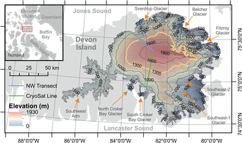
Fig. 1. DIC in the Canadian Arctic Archipelago, its major features and DEM created by the Polar Geospatial Center from DigitalGlobe, Inc. imagery (Porter and others, Reference Porter2018). The location of the two DIC survey lines are shown in blue (NW Transect) and green (CryoSat Line). The orange line is the 1300 m contour, the spatial limit of the study area of this study.
Methods
Surface energy and mass-balance model
We calculate the summer (JJA) surface energy and mass balance of DIC high-elevation area using the model described and calibrated for DIC by Morris and others (Reference Morris2014), a version of which has also been applied to palaeo ice masses (Muschitiello and others, Reference Muschitiello, Pausata, Lea, Mair and Wohlfarth2017). Broadly, the model consists of four modules: surface energy balance; SMB; subsurface percolation and refreezing and vertical temperature flux, operating on a 1-D fixed vertical 1 cm grid.
Meltwater percolation is a complex process which occurs heterogeneously in both space and time. However, the use of 1-D model for investigating firn percolation is widespread and is often used to estimate the SMB of the Greenland and Antarctic ice sheets, and investigate their refreezing capacities (Ettema and others, Reference Ettema2010; Langen and others, Reference Langen, Fausto, Vandecrux, Mottram and Box2017). Models capable of representing the 3-D complexity of meltwater percolation and refreezing on ice sheets do not exist (Verjans and others, Reference Verjans2019). Commonly used 1-D multi-layer snow and firn models often use uneven grid spacing with depth, with thinner layers near the ice surface (e.g. Bougamont and others, Reference Bougamont, Bamber and Greuell2005; Ettema and others, Reference Ettema2010; Langen and others, Reference Langen, Fausto, Vandecrux, Mottram and Box2017). One disadvantage of this approach is that the thickness of an ice layer that is prescribed as impermeable, and that consequently generates runoff, is in-part a function of model set-up and depth. A model schematic is shown in Figure 2. The high uniform vertical resolution is designed to better simulate evolution of ice layers with a range of thicknesses from centimetres to metres at any depth within 10 m of the surface. At the beginning of each summer we use 1000 layers of 0.01 m thickness (Table 1). Our model was calibrated with field measurements of bulk density, snow water equivalent, and snow depth along the CryoSat Line (Fig. 1) by Morris and others (Reference Morris2014) to calculate the optimum values of fresh snow density, fresh snow albedo and bare ice albedo. For a fuller model description and details of the calibration procedure we direct the reader to Morris and others (Reference Morris2014). The details of the runs performed in this study are given in Table 1.
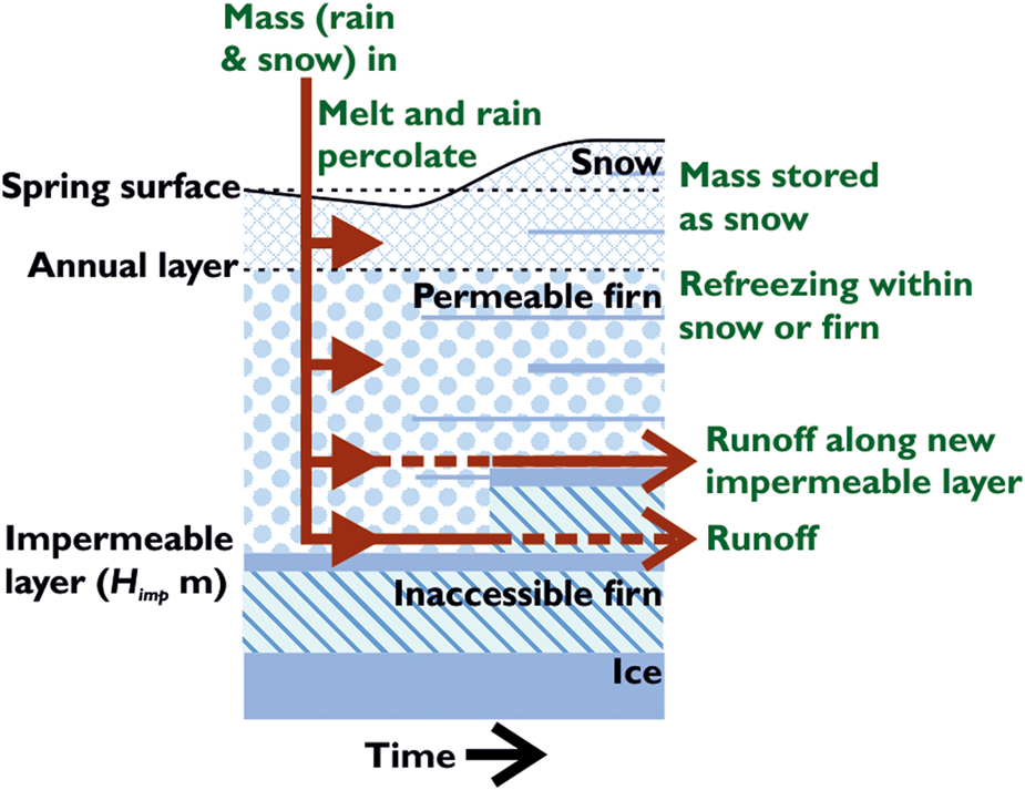
Fig. 2. Model schematic showing the main processes incorporated into the model used in this study.
Table 1. Details of model runs undertaken in this study
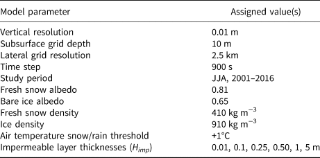
Air temperature snow/rain threshold refers to the air temperature at which precipitation falls as rain. For detailed model description and calibration procedure see Morris and others (Reference Morris2014). The bare ice albedo, fresh snow albedo and fresh snow density as derived by Morris and others (Reference Morris2014) for DIC.
We invoke the model in a spatially distributed manner across DIC, contrasting to Morris and others (Reference Morris2014) who focused on the CryoSat Line in the southwest of the ice cap. A significant addition to the model in this study is the ability to vary the effective percolation depth by prescribing the thickness of the impermeable ice layer at which percolating melt becomes runoff, which we term H imp herein (Table 1). It is important to note here the implicit conflation between impermeable layer thickness and impermeable layer lateral extent necessary in 1-D models. With the inclusion of H imp percolating water is able to bypass ice and access the next available vertical cell unless a continuous ice layer with thickness equal to H imp is encountered. In the event the impermeable layer outcrops at the surface it will become ‘permeable’ again should it thin sufficiently through melting. We choose a regular horizontal grid size of 2.5 km across DIC to allow for a reasonable computation time on a good quality desktop computer. This subaerial resolution is ~3–10 times the ice thickness over the interior of DIC, and so is a suitable distance to average out small scale variability in surface elevation.
With the large variability in potential impermeable layer thicknesses (cf. Bell and others, Reference Bell2008; Machguth and others, Reference Machguth2016) we perform six model runs with H imp = [0.01 0.1 0.25 0.5 1 5] m to sample the potential range of values. At the end of summer we calculate the density profile for the subsequent summer by adding the autumn–winter–spring accumulation above the final (31st August) density profile, and update the impermeable layer depth accordingly.
Model forcing and initialisation
We use a combination of field measurements and a publicly available reanalysis product to force our model. The required inputs are air temperature, downward shortwave radiation, relative humidity, precipitation rate, cloudiness and initial temperature and density profiles.
Field campaigns conducted by the Natural Resources Canada, Geological Survey of Canada (GSC) monitoring programme (Koerner, Reference Koerner2005) on the NW Transect, and as part of the CryoSat Cal/Val project on the CryoSat Line (see Fig. 1), collected air temperature and SMB measurements during our study period. Accounting for refreezing in field SMB monitoring programmes is widely acknowledged to be problematic. The GSC derives SMB following the stratigraphic system (Cogley and others, Reference Cogley2011). In this method, the difference in height between the top of the end-of-summer surface and top of the subsequent end-of-summer surface is measured annually against a survey pole. This value is then converted to net annual SMB (‘net balance’) in water equivalent based on the average density of the material gained or lost at the pole measured. Winter balance is the water equivalent mass of snow accumulation measured each spring above the previous end-of-summer surface. While internal refreezing is not explicitly accounted for, it is estimated that a percentage of the apparent mass loss above the firn line due to summer melt is estimated to be retained within the ice cap as a function of the density of firn in the vicinity of the pole measured. Koerner (Reference Koerner2005) discusses the evolution of the GSC measurements in the Canadian Arctic. Cogley and others (Reference Cogley, Adams, Ecclestone, Jung-Rothenhäusler and Ommanney1995) estimate an uncertainty of 10% for repeat measurements of winter balance from individual pole measurements on White glacier, Axel Heiberg Island. Bell (Reference Bell2008) measures annual snowpack water equivalent (i.e. SMB) multiple times in a 1 km nested grid at sites on the CryoSat Line in 2004 and 2006. Their data suggest that spatial heterogeneity accounts for a further ~10% error. As these errors are unlikely to covary, we estimate a relatively conservative error of 14% for GSC SMB pole measurements.
The NOAA-NCEP North America Regional Reanalysis (NARR) product (Mesinger and others, Reference Mesinger2006) provides the required variables on a ~32 km grid and a 3-hour time step over DIC. For relative humidity, downward shortwave and cloudiness we use the mean of the four NARR nodes within our DIC study area, and linearly interpolate them to the model time step. We assume these variables to be spatially invariant over the study area. However, this approach is not suitable for air temperature and precipitation inputs owing to their pronounced spatial dependencies. Appendix A details how input files of air temperature and precipitation were derived.
We initialise the model density profile in 2001 with firn density measurements collected in 2000/01 (Mair and others, Reference Mair, Burgess and Sharp2005), prior to the mid-2000s extreme warming, and fit an exponential to these data with elevation. The density at the ice cap summit is 436 kg m−3. Above this ‘firn density’ we add the previous September–May snowfall. The temperature profile is initialised every spring by fitting an exponential to a snow surface, and 10 m deep, temperature. We take the temperature at 10 m depth to be the mean of the previous 12 months, and that the surface temperature is equal to the mean May air temperature. This approach means we do not account for the warming of the firn over subsequent summers. In Appendix B we describe sensitivity tests which suggest this has a minor effect on the resultant density stratigraphy. Air temperatures used to calculate initial temperature profiles are derived from NARR as described in Appendix A.
Results
Comparison to field SMB – bulk
We assess our model performance with 241 GSC measurements of SMB during our study period along the NW Transect and the CryoSat line (Fig. 3). We extract modelled SMB in those grid cells along each transect and use a piecewise linear interpolation along the transect to derive a modelled SMB for each H imp value, at the elevation of each measurement point. All model runs have a positive bias (mean difference between the modelled and measured values) and overestimate SMB. Figure 3 shows that H imp = 0.01 m best matches observations, and that bias increases with increasing H imp value.

Fig. 3. Comparison of modelled and measured SMB during our study period (n = 241) for each H imp run, the RMSE and bias (mean difference of modelled and measured values) are also shown.
Comparison to field SMB – spatial-temporal variability
The model successfully reproduces the major multi-annual trends in SMB (Fig. 4), although in general the model overestimates SMB, as indicated by the bulk comparisons to SMB (Fig. 3). We interrogate the spatial results by plotting model output against individual GSC SMB measurements as a function of elevation for all years where field data are available (Fig. 4). With the exception of the H imp = 5 m run, the model generally replicates the quite different patterns of spatial variability in SMB observed along the transect.

Fig. 4. Comparison between measured SMB and modelled SMB on the NW Transect and Cryostat Line (panels a–s), and RMSE for each year (panels t, u) for different H imp values.
Cooler years (2004 and 2013; Fig. 4) display much less variability in SMB with elevation than warmer years (2008 and 2011; Fig. 4). The H imp = 5 m run is clearly incapable of simulating the variability in SMB with elevation seen in warmer years. The measurement variability at SMB stakes is as large as the variability due to assigned model impermeable layer thickness for all other values of H imp from 0.01 to 1 m. The rapid rise in modelled SMB below 1400 m in 2010–2012 on the NW Traverse (Figs 4m to o) is due to melting through of the ice layer established in previous years, making the impermeable layer thickness sufficiently thin to allow percolation into previously sealed-off pore space. By considering our modelled-measured SMB pairs along the two survey transects by year we can consider the quality of the model fit to observations in each year. Figures 4t to u shows the root mean square error (RMSE) for each year where observations are available. In the majority of years we see H imp = 0.01 m performs best compared to survey data.
Modelled SMB and SMB components
The modelled DIC study area SMB and primary SMB components averaged over the study area are shown in Figure 5. As expected the SMB of the study area is positive for all years, with the exception of 2011, and for smaller H imp values in 2008 and 2016 (Fig. 5a).

Fig. 5. Average modelled SMB and SMB components for the study area.
The variation in SMB in response to H imp value is a function of both runoff and refreezing. In later years (2010 onwards) runoff becomes more tightly coupled to melt, whereas in 2006–2010 some variation exists. This is due to the densification of the lower accumulation area becoming less capable of retaining meltwater. Melt varies slightly between H imp runs owing to small variations in the albedo due to the surface density. Discounting the end-member H imp = 5 m (given its poor match with both temporal and spatial patterns of observations above), varying H imp from 0.01 to 1 m increases the cumulative SMB of the study area by 18% over the study period.
We analyse these data further to investigate the location of this refreezing within our model. We highlight the distinction between total refreezing and mass retention. The same material can melt and refreeze multiple times in a season, contributing to total refreezing, whereas mass retention accounts for internal accumulation. We adopt a simple division of mass retention as that taking place within the annual snowpack and that beneath the annual layer. This distinction is important because if refreezing only takes place in the annual snowpack, it is sustainable as the subsequent winter accumulation replenishes pore space, and thus does not lead to net reduction in refreezing capacity.
The mean fraction of all internal accumulation occurring within the annual snowpack for H imp values 0.01, 0.1, 0.25, 0.5 and 1 m are 0.66, 0.52, 0.49, 0.46 and 0.45 respectively over the period 2001–2016 (Fig. 6a). Therefore, on average, approximately half the mass retention takes place within the annual snowpack, which is replenished each year by winter snowfall. Figure 6a also demonstrates significant interannual variation in the location of refreezing. In less-positive (warmer) SMB years a very small fraction of mass retention takes place within the annual snowpack, while in more positive (cooler) years (2013) almost all refreezing takes place in the snowpack, even after a period of extreme melt. The spatial and temporal (presented as 4-year means) variation of fractional mass retention taking place in the annual snowpack is presented in Figures 6b to e. These data show distinct ring-like patterns of percolation due to elevation-dependent air temperature, the accumulation pattern and the development of impermeable layers.
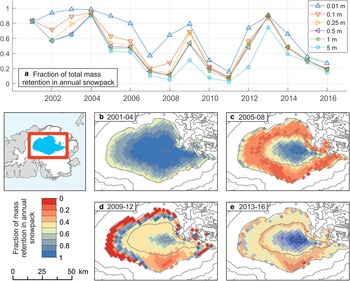
Fig. 6. Temporal and spatial distribution of mass retention taking place within the annual snowpack. Panel a is the yearly mean, and panels b–e are 4-yearly means excluding the end member H imp = 0.01 and 5 m runs. Elevation contours spaced at 300 m as in Figure 1 are provided for reference.
In the years before the mid-2000s warming, the majority of mass retention is in the annual snowpack (Fig. 6b). During the next 4-year period retention occurs in the annual snowpack above 1600 m while multi-year firn pore space is preferentially infilled in the lower accumulation zone (Fig. 6c). In the following time periods the pattern of refreezing becomes more complex owing to the development of impermeable layers and the potential for accumulation as superimposed ice (Koerner, Reference Koerner1970). Figure 6d shows that no retention on the westerly and northerly margins of the study area occurs in the snowpack, as surface melting removes the entire annual snowpack. In the southeast of the study area the high snowfall means some snow survives the melt season down to 1300 m. Immediately adjacent to this marginal zone is a band where mass is preferentially retained in the snowpack. Here, some winter accumulation survives the melt season, but subsurface impermeable layers are established, and meltwater can only either refreeze in the snowpack as infiltration ice, accumulate as superimposed ice or runoff. For the majority of the study area mass retention occurred approximately equally, but close to the summit mass is still preferentially retained in the snowpack. In the final 4-year period winter accumulation in the lower accumulation area has begun to be maintained over the melt season, resuming mass retention (Fig. 6e).
Comparison to measured stratigraphy – GPR and bulk density
We further assess model performance by comparing the modelled evolution of near-surface density stratigraphy to observations based on interpretation of GPR surveys, and to measurements of the mean density of the uppermost 2.5 m of the snow/firn column.
Gascon and others (Reference Gascon, Sharp, Burgess, Bezeau and Bush2013a) report longitudinal GPR profile observations of the development of a near-surface reflection-poor zone along the CryoSat Line, which is interpreted to be the development of a thick near-surface ice layer. Gascon and others (Reference Gascon, Sharp, Burgess, Bezeau and Bush2013a) report that by 2012 the thickness of this ice layer had grown to 0.73 ± 0.11 m at 1610 m, 3.85 ± 0.16 m at 1490 m and 5.67 ± 0.18 m at 1400 m. We recreate a pseudo-transect along the same course using spring density profiles from our model output (Fig. 7). By selecting the density profiles with depth along the transect we see the development of comparable near-surface ice layers with time for different H imp values.

Fig. 7. Spring density profiles along the approximate course of the CryoSat survey line for four time slices (columns) for different Himp values (rows).
Our model results indicate that the near-surface of DIC above 1300 m has undergone a fundamental change in density structure over our study period. A thin impermeable layer fails to produce any significant quantity of continuous near-surface ice (Figs 7a to h). The intermediate H imp values (0.25, 0.5 and 1 m), shown in Figures 7i to t, however recreate comparable ice layers. Percolation when H imp = 5 m results in near-surface ice layers many metres thick in 2012, ~3 m thick at 1444 m and >6 m thick at 1321 m in 2012 (Figs 7u to x). Note that, we use a pure ice density of 910 kg m−3 to define impermeability but, in actuality, ice can be impermeable at densities less than this. We would expect that a smaller ‘impermeable’ density would increase runoff and reduce deep percolation. This may explain why our H imp = 5 m run performs poorly when compared to SMB, but reasonably well when compared to radar stratigraphy. Machguth and others (Reference Machguth2016) measure the densities of ~5 m thick ice layers in the lower accumulation zone of the Greenland ice sheet (see their Fig. 2) and find densities close to the density of pure ice but with several pockets of ice closer to ~850 kg m−3. The ice layer observed in GPR by Gascon and others (Reference Gascon, Sharp, Burgess, Bezeau and Bush2013a) shows visible structure and so is unlikely to be solid bubble-free ice and will contain gas inclusions, and remnant pockets of firn which were not saturated with meltwater before refreezing. Therefore, our model likely underestimates the thickness of near-surface ice layers as would be observed.
With our model we are able to extend discussion beyond that of Gascon and others (Reference Gascon, Sharp, Burgess, Bezeau and Bush2013a) and consider post-2012 layer development. For H imp = 0.25–1 m, we see that between 2012 and 2016 the changes in firn stratigraphy at lower elevations are relatively minor owing to self-limiting behaviour (i.e. the balance between surface lowering through melt, runoff and percolation). In all model runs we see a partial replenishment of pore space within ~2 m of the surface at higher elevations.
Bezeau and others (Reference Bezeau, Sharp, Burgess and Gascon2013) provide measurements of the density of the top 2.5 of the firn column at sites on DIC above 1300 m. Note that there is a conflict in the naming conventions between the sites of Colgan and others (Reference Colgan, Davis and Sharp2008) and those visited by Bezeau and others (Reference Bezeau, Sharp, Burgess and Gascon2013). Consequently, we use data from Bezeau and others (Reference Bezeau, Sharp, Burgess and Gascon2013) on the CryoSat Line where we can be confident of the measurement's location. Figure 8 shows the spring 2012 bulk near-surface (top 2.5 m) density plotted against modelled values for each H imp value. All model runs, except for H imp = 0.01 m, underestimate high densities and overestimate lower densities. In this comparison H imp = 0.25 m best fits the data, with the smallest mean difference between modelled and measured density and the smallest RMSE.

Fig. 8. A comparison of measured near-surface density (top 2.5 m) along the CryoSat Line as reported by (Bezeau and others, Reference Bezeau, Sharp, Burgess and Gascon2013) and density of the top 2.5 m as modelled in this study.
Discussion
Sensitivity of SMB to impermeable layer thickness
Although SMB is relatively insensitive to a wide range of impermeable ice layer thicknesses, our results indicate that allowing very thick ice layers to be permeable to percolating meltwater leads to unrealistically positive SMB, evidenced by the H imp = 5 m runs having poor agreement with observations of both temporal and spatial patterns in SMB (Fig. 4). Discounting this run, cumulative SMB 2001–16 can vary by 18% across our study area as a function of the assigned impermeable layer thickness. Previous studies (e.g. van Angelen and others, Reference van Angelen2013) state that density structure is important to the refreezing capacity of Greenland. In this study however, we can validate our results against localised field data, as opposed to ice-sheet wide measurements, and assess how well refreezing processes are represented across the high elevation regions of an Arctic ice mass. It is important to highlight that although our study area encompasses the vast majority of the actual accumulation area over the time period from 2001 to 2016, it covers only ~21% of the area of DIC. This contrasts to Greenland where ~80% of the ice-sheet area is within the accumulation area (Vernon and others, Reference Vernon2013), and so we propose the sensitivity of the entire ice sheet's SMB to H imp will be considerably greater there.
Near-surface impermeable ice layers
Our model-led interpretation of near-surface ice layer formation agrees with that led by a longitudinal study of DIC GPR stratigraphy (Gascon and others, Reference Gascon, Sharp, Burgess, Bezeau and Bush2013a). These authors observed an initial deep percolation and then a growth by vertical accretion. In Figure 7 we see the formation of thinner ice layers, then an infilling of the interleaving pore space during intense melt years. Gascon and others (Reference Gascon2014) used CROCUS (Vionnet and others, Reference Vionnet2012) to model the density development 2004–10 at sites on the CryoSat Line, and observed that this model overestimated density in the near-surface. This is despite the fact that these CROCUS runs allowed water to percolate through ice layers. Thus, they attribute this near-surface positive mass balance to a lack of preferential flow paths in the model. Our model, on the basis of the comparison presented here, does not obviously exhibit a similar bias. One possibility for this is that Morris and others (Reference Morris2014) implicitly account for the enhanced densification due to vertical flow of meltwater via preferential flow paths in their Monte Carlo calibration against bulk density, snow water equivalent and snow depth. Other possibilities for mismatch may be due to spatial variations in lateral low, subsurface melting through ice layers, in addition to the development of preferential flow paths. These results also demonstrate that the near-surface ice layers are maintained by a balance between melting and percolation in the lower accumulation area, and so the maximum layer thickness is not necessarily at the lowest elevation. Once a near-surface ice layer is established a balance between melting and percolation limits its thickness. Through consideration of both SMB and stratigraphy our study therefore identifies a narrower range of optimal values for H imp between 0.25 and 1 m that can simulate both interannual and spatial variability in SMB, and the evolution of near-surface density structure.
Runoff, refreezing and resilience
We consider the location where refreezing is taking place by using a simple classification of mass retention which takes place in the annual snowpack, and that in the multi-year firn. For around half of the study area, mass retention takes place in the annual snowpack. Discounting the end member H imp = 5 m run, 45–66% of mass retention takes place in the annual snowpack, but significant interannual variability exists. Using the narrower band of H imp (0.25 and 1 m) values identified above 45–49% of mass retention takes place within the annual snowpack. In all model runs we see a replenishment over the high elevation snowpack after ~2012 (Fig. 7), indicating some resilience to future isolated warm years. Our modelling suggests that one or two cooler years can restore a meaningful proportion of lost runoff buffering capacity. By comparing Figures 7o, p to 7s, t we see the burial of the impermeable layer, but a large increase in buffering capacity formed over 2 years. This conclusion is reliant on the accuracy of our precipitation and net accumulation fields away from survey transects, which are poorly constrained, particularly in the southeast of our study area (see Appendix A). This finding has major implications for projecting the long term changes in buffering capacity of the accumulation area of larger scale ice masses such as the Greenland ice sheet and implies that it is important to accurately model how the magnitudes and proportions of refreezing vary with depth, rather than basing calculation of pore space volume for refreezing on maximum percolation depths. This further highlights the importance of improved understanding of controls on (e.g. Colgan and Sharp, Reference Colgan and Sharp2008), and spatial patterns of precipitation and accumulation (e.g. Sylvestre and others, Reference Sylvestre, Copland, Demuth and Sharp2013) across the high elevation regions of polar ice masses; since this replenishes snowpacks and may restore a large proportion of the ice mass's buffering capacity.
Implications and outlook
Field evidence shows that impermeable layers are generated in the long-term accumulation areas of polar ice masses (Gascon and others, Reference Gascon, Sharp and Bush2013b; Machguth and others, Reference Machguth2016), but also that the near-surface of these ice masses also exhibit extreme horizontal heterogeneity (Bell and others, Reference Bell2008; Brown and others, Reference Brown, Harper, Pfeffer, Humphrey and Bradford2011). At present the use of 1-D models at km scale horizontal resolution to estimate SMB is widespread due to the large domain sizes required and the computational demands necessary. This raises the question of how to represent laterally heterogeneous percolation in these models, for example the cumulative SMB difference between H imp = 0.01 m and H imp = 5 m is a 48% increase in our model. In totality, our results imply that, while ice is undoubtedly impermeable, water should be allowed to bypass <0.25 m thick ice layers in 1-D models, but not 1 m thick ice layers. We arrive at this range because high H imp values clearly fail to simulate measured SMB and low H imp values clearly fail to recreate firn properties (bulk density and density stratigraphy, as interpreted from GPR imagery). The cumulative SMB difference between H imp runs with 0.25 and 1 m is 6%. Importantly, the experiment which best agrees with field data is different depending on whether the model is compared to SMB or subsurface properties. In this study we assume that the calibration procedure of Morris and others (Reference Morris2014) is correct and only vary the impermeable layer thickness. In reality, compensating errors in the full model flow from start to finish, particularly in relation to the uncertain input parameters (see the Appendix) and parameterisations of natural processes, may be present and act against each other in the model. Regardless the conclusion that the parameterisation of impermeable layer thickness has a major effect on the output of our model is instructive. Caution must be exercised when interpreting refreezing properties from tipping bucket models or models with varying model layer thicknesses which have been tuned to, or compared to SMB measurements, and not firn properties.
In the Kangerlussuaq region of Greenland two recent studies have considered impermeable layer thickness in a related way. Charalampidis and others (Reference Charalampidis2015) used firn core observations from Machguth and others (Reference Machguth2016) to stop vertical percolation past an ice layer thickness of 6 m at the KAN_U site at 1840 m elevation. Whereas van As and others (Reference van As2017) used an impermeable layer thickness of 1 m in a study of the Watson River catchment. DIC represents an excellent type site for investigating the firn response to extreme melting in a warming climate owing to the relative wealth of field data. We advocate therefore, for further detailed model-data comparisons. Distributed radar studies have been of particular use for extrapolating away from survey sites or transects (e.g. de la Peña and others, Reference de la Peña2015; Steger and others, Reference Steger2017). On DIC Rutishauser and others (Reference Rutishauser2016) inferred near-surface (in)homogeneity in spring 2014 from the scattering component for surface reflection using a 60 MHz airborne radar. In this work the summit region is relatively low-scattering (homogeneous; fewer near-surface ice layers), the mid-elevations are high-scattering (inhomogeneous; numerous near-surface ice layers) and low elevations are low scattering (homogeneous; solid ice). Qualitatively this agrees with our modelling results. Figure 7 shows that between 2014 and 2016 relatively ice-layer free stratigraphy develops at higher elevations on DIC, while the lower study area is predominantly composed of relatively homogeneous high-density ice.
Van Wychen and others (Reference van Wychen2017) showed that major DIC glaciers exhibited velocity variations tens of kilometres from their termini, some which are concurrent with one another suggesting a common atmospheric or oceanic forcing mechanism. Clason and others (Reference Clason, Mair, Burgess and Nienow2012) modelled the delivery of meltwater to the ice bed on Croker Bay glacier (Fig. 1) and concluded that the rate of meltwater delivery to crevasses to be the main control on the ability of water to reach the ice bed and enhance basal motion. Cook and others (Reference Cook2019) show that the retreat of frontal position in the Canadian Arctic Archipelago is correlated with an increase in air temperature. The widespread development of impermeable near-surface layers fundamentally changes the surface hydrology of DIC and, therefore, may affect surface flow routing to moulins and fractures in the lower catchment. One avenue for future work could be to investigate relationships between changing (near-)surface hydrology and DIC dynamic response.
Conclusions
We have reported the first systematic assessment of an impermeable layer thickness parameterisation in a 1-D snow and firn model, and assessed model performance using field SMB measurements, published GPR profiles and measurements of near-surface bulk density. We have shown that for a range of impermeable layer thickness in line with those discussed in the literature (0.01–5 m) the cumulative study area SMB can vary by 48% over the study period. Dye tracing by Bell and others (Reference Bell2008) observe percolation apparently limited by a 1–2 cm ice layer at 1800 m on DIC, while Machguth and others (Reference Machguth2016) discuss ice layers many metres thick inducing runoff. Furthermore, percolation and refreezing models that use varying layer thicknesses may not know how thick a modelled ice layer is that stops vertical percolation. Using field survey data and published GPR profiles we have identified a narrower range of realistic H imp values of 0.25–1 m, over which the cumulative study area SMB varies by only 6%. The optimal H imp value differs depending on whether the model is compared to SMB or subsurface properties. We advocate that future studies of high elevation SMB and refreezing using 1-D models integrate these findings, and where possible use a range of field data (including SMB; precipitation; subsurface properties) to inform their experimental design and evaluation. We do not categorically recommend an impermeable layer thickness for universal use in similar models as the thickness of such an impermeable layer is likely dependent on regional factors, such as the thermal regime, the melt flux and pre-existing structural weaknesses. We model and discuss the formation mechanism of thick, likely impermeable, near-surface ice layers which appear to form after an initial deep percolation that creates thinner decimetre-scale infiltration ice layers. The pore space between these is then progressively infilled to become a quasi-continuous layer several metres thick. Once formed the thickness of the layer is self-limited in the lower accumulation area by surface melting, and percolation and refreezing beneath it. In order to grow by vertical accretion accumulation must outpace lowering due to surface melting. Our model results suggest that after a period of intense melt in the 2000s, a partial recovery of high elevation near-surface firn during cooler summers provided some buffering to future, isolated intense melt years. We underline that the robustness of this conclusion on DIC depends on the uncertain precipitation field away from survey transects where output can be more thoroughly compared to field data. Regional climate model evidence indicates that a long-term decrease in firn buffering capacity of ice caps in the Canadian Arctic is expected (Lenaerts and others, Reference Lenaerts2013). Understanding this recovery and potential resilience through improved knowledge of precipitation, percolation and refreezing processes is key for projecting the future of the accumulation areas of Arctic ice masses that, although they are likely to experience long-term trend of climatic warming, will nonetheless periodically experience cooler, more positive mass-balance years.
Acknowledgements
Thanks to the University of Liverpool ECR and Returners Fund whose award to DA advanced this work. ArcticDEM provided by the Polar Geospatial Center under NSF OPP awards 1043681, 1559691 and 1542736. Thanks to the Editor, William Colgan, and the two anonymous reviewers for their comments which led to a much-improved manuscript.
Author contributions
DA and DM designed the study and interpreted results. DA performed the simulations, analysis and drafted the manuscript. DB provided field data and advised on model forcing. All authors contributed to discussions and manuscript editing.
Appendix A: Model forcing and initialisation
We use near-continuous air temperature measurements at 1781 m elevation on the NW Transect since 2004 for the primary model air temperature forcing.
For summers 2001–2003 we adjust the air temperature at the nearest NARR model node to the AWS site with their mean difference, such that T AWS = T NARR − 2. Comparison of concurrent NARR and AWS air temperatures shows that NARR underestimates summer high air temperatures and overestimates summer low temperatures over DIC. We found that a simple static adjustment of the NARR temperatures maintains a frequency distribution close to 0°C similar to that which is measured, relative to a correction method based on Gardner and Sharp (Reference Gardner and Sharp2009). The relationship between adjusted NARR and AWS for the overlapping period is shown in Figure 9.

Fig. 9. A comparison of summer adjusted NARR 2 m air temperature and AWS measured 2 m temperatures. NARR only used for three summers (2001–2003) for which AWS air temperature data were not available.
In both cases we use a uniform mean measured temperature lapse rate of −0.0057°C m−1 and ArcticDEM (Porter and others, Reference Porter2018) to distribute the temperature field. This is therefore not sensitive to temperature inversions or gradients in air temperature not due to elevation. Inspection of MODIS-derived mean summer surface temperatures 2000–15 (Mortimer and others, Reference Mortimer, Sharp and Wouters2016; Fig. 2 therein) indicates elevation is the primary driver of DIC surface temperature distribution. This lapse rate was calculated from the accumulation area daily mean temperature summer lapse rates on the NW Transect, where concurrent measurements are available at elevations of 1781 and 1317 m, and at one or both at 1731 or 1594 m. An approach based on the dynamic lapse rate method proposed by Gardner and Sharp (Reference Gardner and Sharp2009) yielded a mean lapse rate of 0.0049°C m−1. As their method was conceived for the whole elevation range (whereas here we focus on the ice cap area above 1300 m a.s.l.) we elect to use the measured mean lapse rate.
In our model implementation we require precipitation input for the winter accumulation (i.e. the spring snow thickness) and the summer precipitation rate. Koerner (Reference Koerner1966) noted winter accumulation is 1.5–2 times more in the SE of the DIC accumulation area, based on three springtime traverses. Shepherd and others (Reference Shepherd, Du, Benham, Dowdeswell and Morris2007) suggest a significant EW gradient of accumulation on DIC. NARR fails to capture this pattern in summer or winter accumulation. Recent work by Noël and others (Reference Noël2018) applied a regional climate model and a 1-D tipping bucket snow and firn (Ettema and others, Reference Ettema2010) scheme to the Canadian Arctic Archipelago. One option would be to use their precipitation output to force our model. Noël and others (Reference Noël2018) bilinearly interpolate RACMO2 precipitation output at 11 km resolution to 1 km over the whole Canadian Arctic Archipelago. To assess its suitability for our study, we plot the 1 km RACMO2 2001–16 precipitation to examine its spatial pattern (Fig. 11a). This exercise demonstrates that RACMO2 does not resolve the strong spatial gradient observed by field investigations (Koerner, Reference Koerner1966). Noël and others (Reference Noël2018) demonstrate that, at several points, RACMO2 after adjustment using a statistical downscaling technique, overestimates GSC SMB in most of the high elevation region of the DIC NW Transect by ~100 kg m−2 a−1 (see their Fig. S3b). A lack of knowledge on precipitation in the Canadian Arctic is acknowledged as a limitation in their study.
A further test of the suitability of RACMO2 for these purposes is to compare SMB output with core-derived SMB over a period before extreme melt and the major changes in firn stratigraphy in the mid-late 2000s (Bezeau and others, Reference Bezeau, Sharp, Burgess and Gascon2013; Gascon and others, Reference Gascon, Sharp, Burgess, Bezeau and Bush2013a). At this time, we might expect that SMB is more reflective of the precipitation pattern. For this, we use core derived mean SMB for 1963–2003 (Mair and others, Reference Mair, Burgess and Sharp2005; Colgan and others, Reference Colgan, Davis and Sharp2008) at 13 sites above 1300 m on DIC, and compare them to the 1963–2003 mean SMB from the nearest RACMO2 node. As far as we are aware these are the only spatially distributed, coincident measurements of SMB across the high-elevation area of DIC. In the interests of reproducibility please note that the correct positions of the cores CD and CE in Colgan and others (Reference Colgan, Davis and Sharp2008) Table 2 are at 75.45 N, 82.53 W; and 75.24 N, 82.03 W respectively (personal communication from W. Colgan, 2018). The core-derived SMB and RACMO2 SMB show poor agreement and have a correlation coefficient of −0.42 (Fig. 10).

Fig. 10. A comparison of average SMB (1963–2003) from firn cores (Mair and others, Reference Mair, Burgess and Sharp2005; Colgan and others, Reference Colgan and Sharp2008) and average SMB (1963–2003) modelled using a regional climate model (Noël and others, Reference Noël2018) at 13 sites >1300 m elevation prior to the extreme mid-2000s warming.
When faced with this apparent mismatch we design a non-physical spatial scaling in which precipitation is 1.75× higher in the SE, than in the NW and decreases radially and normally (σ = 12.5 km; Fig. 11b). We derive the mean spring snow depth from measurements at 1781, 1751 and 1731 m elevation on the NW Transect and scale according to this pattern over the study area.

Fig. 11. (a) The mean annual (2001–2016) precipitation field from RACMO2 (Noël and others, Reference Noël2018); and (b) the mean annual precipitation field (2001–2016) used in this study, as guided by field traverses (Koerner, Reference Koerner1966).
Little is known about DIC summer precipitation both spatially and temporally, since ice riming and consequent discontinuities in measurements records make the interpretation of sparse AWS sonic ranger data non-trivial, as precipitation occurs alongside melting, refreezing and densification processes which also alter the surface height. Therefore, we use NARR output and assume that the spatial distribution of summer precipitation is identical to that of the winter accumulation. Gascon and others (Reference Gascon2014) report that NARR overestimates precipitation by 30–50% on the CryoSat Line. Considering this, we take the NARR precipitation rate closest to the top of the NW Transect and CryoSat Line (Fig. 1), reduce all NARR accumulation values by 40% and scale spatially according to the winter balance pattern to derive the distributed summer precipitation rate.
Appendix B: Effect of firn temperature
In order to use the measured spring snow depths, we took a simple approach to firn temperature, rather than assume an accumulation rate through the winter which would affect the snow/firn temperature. In our approach we assign a firn temperature profile at the start of each summer based on the assumption that the mean annual air temperature equals the firn temperature at 10 m (see the ‘Methods’ section). This is a reasonable assumption early in our study period when the very little melt and refreezing takes place in the dry snow zone. However, as a consequence of this, firn warming due to latent heat release during one summer is not carried over to the subsequent summer. This means we do not account for the longer-term firn warming, which will likely have an effect on the refreezing behaviour later on in the study period. Bezeau and others (Reference Bezeau, Sharp, Burgess and Gascon2013) show that on the CryoSat Line in Spring 2012 the 10 m firn temperature was several degrees higher than the mean annual air temperature. The 10 m firn temperatures were approximately: −17.7°C at 1755 m; – 14.7°C at 1640 m and −12.8°C at 1511 m. To assess this sensitivity of our model to these observations, we re-run our model in 2012 at three grid cells on the CryoSat Line with similar elevations: 1759, 1636 and 1492 m. In these runs we set the 10 m temperature to that measured at the nearby corresponding location and the snow surface temperature to the spring temperature (−13.0; −12.3 and −11.5°C respectively; see the ‘Methods’ section) and linearly fit between these two end members over the depth range. This method may overestimate the near-surface temperature as we do not account for the conduction of the winter cold wave but is suitable as we aim to assess the sensitivity of the model to elevated snow/firn temperatures.
At the two higher elevation sites we find this change has a minor effect on SMB. The warmer snow/firn run produces a slightly less positive summer SMB: a mean decrease of 0.47 kg m−2 at 1759 m, and 3.2 kg m−2 at 1636 m. At 1492 m however the warmer snow/firn results in a mean summer SMB that is less negative by 9.3 kg m−2. At this site early in the season, the warmer run produces more runoff due to less refreezing, and deeper percolation reaching the impermeable layer. However, later in the season the cold snow/firn run produces more runoff due to the formation of a shallower impermeable ice layer and its outcropping at the surface, where its lower albedo results in more melting. Variations of this magnitude are minor when considered with the along-transect variation in SMB by year but would accumulate for longer study periods looking at the multi-decadal cumulative mass loss from DIC (Fig. 4). This test suggests that the SMB of the lower-intermediate sections of the DIC long-term accumulation zone are most sensitive to long-term firn warming.
In terms of the resultant density stratigraphy we compare the density daily time series for the intermediate H imp = 0.5 m run. Figure 12 shows that, as expected, the warmer snow/firn temperatures result in deeper percolation and refreezing. The density of some cells is increased by <200 kg m−3 due to refreezing in the warm snow/firn run relative to the cold snow/firn run (Figs 12c, f and i). A thin ice layer very close the glacier surface is formed at the lowest elevation site. Critically, however, the fundamental pattern of refreezing and resultant stratigraphy remains unchanged indicating that the seasonal input of latent heat is more important than the initial spring firn temperature profile in determining stratigraphy.

Fig. 12. The sensitivity of the modelled daily density stratigraphy at three elevations on the CryoSat Line for JJA 2012, using the firn temperature initialisation method outlined in Methods (a, d, g), and an elevated temperature profile based on measurements (Bezeau and others, Reference Bezeau, Sharp, Burgess and Gascon2013; b, e, h). The difference between the two scenarios are shown (c, f, i).


 Open access