Birational geometry of symplectic quotient singularities

Abstract

For a finite subgroup $\Gamma \subset \mathrm {SL}(2,\mathbb {C})$ and for $n\ge 1$, we use variation of GIT quotient for Nakajima quiver varieties to study the birational geometry of the Hilbert scheme of n points on the minimal resolution S of the Kleinian singularity $\mathbb {C}^2/\Gamma$. It is well known that $X:={{\,\mathrm{{\mathrm {Hilb}}}\,}}^{[n]}(S)$ is a projective, crepant resolution of the symplectic singularity $\mathbb {C}^{2n}/\Gamma _n$, where $\Gamma _n=\Gamma \wr \mathfrak {S}_n$ is the wreath product. We prove that every projective, crepant resolution of $\mathbb {C}^{2n}/\Gamma _n$ can be realised as the fine moduli space of $\theta$-stable $\Pi$-modules for a fixed dimension vector, where $\Pi$ is the framed preprojective algebra of $\Gamma$ and $\theta$ is a choice of generic stability condition. Our approach uses the linearisation map from GIT to relate wall crossing in the space of $\theta$-stability conditions to birational transformations of X over $\mathbb {C}^{2n}/\Gamma _n$. As a corollary, we describe completely the ample and movable cones of X over $\mathbb {C}^{2n}/\Gamma _n$, and show that the Mori chamber decomposition of the movable cone is determined by an extended Catalan hyperplane arrangement of the ADE root system associated to $\Gamma$ by the McKay correspondence. In the appendix, we show that morphisms of quiver varieties induced by variation of GIT quotient are semismall, generalising a result of Nakajima in the case where the quiver variety is smooth.

1 Introduction

For a finite subgroup $\Gamma \subset \mathrm {SL}(2,\mathbb {C})$, let $S\rightarrow \mathbb {C}^2/\Gamma$ denote the minimal resolution of the corresponding Kleinian singularity. The well-known paper by Kronheimer [44] realises S as a hyperkähler quotient, describes the ample cone of S as a Weyl chamber of the root system of type ADE associated to $\Gamma$ by the McKay correspondence, and constructs the simultaneous resolution of the semi-universal deformation of $\mathbb {C}^2/\Gamma$. In the present paper we provide a natural generalisation of these results to higher dimensions by studying symplectic resolutions of the quotient singularity $\mathbb {C}^{2n} / \Gamma _n$ for any $n\ge 1$, where $\Gamma _n=\Gamma \wr \mathfrak {S}_n$ is the wreath product. We prove that every projective crepant resolution of $\mathbb {C}^{2n} / \Gamma _n$ can be realised as a Nakajima quiver variety, generalising the description of the Hilbert scheme $X:={{\,\mathrm{{\mathrm {Hilb}}}\,}}^{[n]}(S)$ of n-points on S by Kuznetsov [45] (established independently by both Haiman and Nakajima). We also obtain a complete understanding of the birational geometry of X over $\mathbb {C}^{2n} / \Gamma _n$ by describing explicitly the movable cone of X over $\mathbb {C}^{2n} / \Gamma _n$ in terms of an extended Catalan hyperplane arrangement determined by the ADE root system associated to $\Gamma$. Finally, we construct, using quiver GIT, the simultaneous resolution of the universal Poisson deformation of $\mathbb {C}^{2n}/\Gamma _n$.

1.1 Quiver varieties and the linearisation map

For $n\ge 1$ and for a finite subgroup $\Gamma \subset \mathrm {SL}(2,\mathbb {C})$, the symmetric group $\mathfrak {S}_n$ acts on the direct product $\Gamma ^n$ by permuting the factors, and the wreath product is defined to be the semidirect product $\Gamma _n:= \Gamma ^n\rtimes \mathfrak {S}_n\subset \mathrm {Sp}(2n,\mathbb {C})$. Throughout the introduction, we assume $n > 1$ and $\Gamma$ is non-trivial (see Sect. 4.4, Remark 7.8 and Proposition 7.11 for these degenerate cases). It is well-known that the Hilbert scheme of n points on S provides a symplectic resolution

$$\begin{aligned} f:X:={{\,\mathrm{{\mathrm {Hilb}}}\,}}^{[n]}(S)\longrightarrow Y:=\mathbb {C}^{2n}/\Gamma _n \end{aligned}$$

of the corresponding quotient singularity. In particular, f is a projective, crepant resolution of singularities.

In order to study the birational geometry of X over Y, we first recall that X can be constructed by GIT as a quiver variety. Consider the affine Dynkin graph associated to $\Gamma$ by McKay [55], where the vertex set is by definition the set of irreducible representations of $\Gamma$. Define the dimension vector $\varvec{v}:= n \delta$ and the framing vector $\mathbf {w}= \rho _0$, where $\delta$ and $\rho _0$ are the regular and trivial representations of $\Gamma$ respectively. If we write $R(\Gamma )$ for the representation ring of $\Gamma$, then our interest lies in studying the quiver varieties $\mathfrak {M}_\theta := \mathfrak {M}_\theta (\varvec{v},\mathbf {w})$, where the GIT stability parameter $\theta$ can be regarded as an element in the rational vector space $\Theta :={{\,\mathrm{\mathrm {Hom}}\,}}(R(\Gamma ),\mathbb {Q})$; equivalently, $\mathfrak {M}_\theta$ can be regarded as a moduli space of $\theta$-semistable $\Pi$-modules, where $\Pi$ is the framed preprojective algebra of $\Gamma$ (see Sect. 3.1 for details). A result of Kuznetsov [45] (also due to Haiman [34] and Nakajima [57]) determines an open GIT chamber $C_-$ in $\Theta$ and a commutative diagram

for any $\theta \in C_-$, where the horizontal arrows are isomorphisms and where the right-hand symplectic resolution is obtained by variation of GIT quotient.

Our first main result calculates explicitly the GIT chamber decomposition of $\Theta$ and describes the geometry of the quiver varieties $\mathfrak {M}_\theta$ whenever $\theta$ lies in a chamber. To state the result, write $\Phi ^+$ for the set of positive roots in the ADE root system of finite type associated to $\Gamma$ by the McKay correspondence, and for $\gamma \in R(\Gamma )$ we write $\gamma ^\perp := \{\theta \in \Theta \mid \theta (\gamma )=0\}$ for the dual hyperplane.

Theorem 1.1

For $\theta \in \Theta$, the following are equivalent:

• (i) $\theta$ is generic, i.e. $\theta$ is contained in a GIT chamber;

• (ii) $\theta$ does not lie in any hyperplane from the hyperplane arrangement

  $$\begin{aligned} \mathcal {A}:= \big \{ \delta ^\perp , (m\delta \pm \alpha )^\perp \mid \alpha \in \Phi ^+, \ 0 \le m < n \big \}; \end{aligned}$$

• (iii) the morphism $f_\theta :\mathfrak {M}_\theta \rightarrow \mathfrak {M}_0$ obtained by variation of GIT quotient is a projective crepant resolution.

In particular, for any such $\theta \in \Theta$, there is a birational map $\psi _\theta :X\dashrightarrow \mathfrak {M}_\theta$ over Y that is an isomorphism in codimension-one.

As a result, taking the proper transform along $\psi _\theta$ enables us to identify canonically the Néron–Severi spaces of X and $\mathfrak {M}_\theta$ for any generic $\theta$, so we may regard the ample cone of $\mathfrak {M}_\theta$ as lying in $N^1(X/Y)$.

In order to understand the birational geometry of X, we exploit the link between wall-crossing for stability parameters and birational transformations of quiver varieties provided by the linearisation map arising from the GIT construction of $\mathfrak {M}_\theta$. To define this map, let C be any GIT chamber in $\Theta$ and fix $\theta \in C$. The quiver variety $\mathfrak {M}_\theta$ comes equipped with a tautological locally-free sheaf $\mathcal {R}:= \bigoplus _{i\in I} \mathcal {R}_i$, where the summand $\mathcal {R}_i$ has rank $v_i$ for each vertex $i\in I$ in the framed affine Dynkin graph (see Sect. 3.4). The linearisation map for the chamber C is the $\mathbb {Q}$-linear map

$$\begin{aligned} L_C:\Theta \longrightarrow N^1(X/Y) \end{aligned}$$

defined by sending $\eta = (\eta _i)_{i\in I}$ to the class of the line bundle $L_C(\eta ) = \bigotimes _{i\in I} \det (\mathcal {R}_i)^{\otimes \eta _i}$. Theorem 1.1 is a key ingredient in enabling us to prove that $L_C$ is a linear isomorphism that identifies the chamber C with the ample cone $\mathrm {Amp}(\mathfrak {M}_\theta /Y)$ for $\theta \in C$. In order to understand how the linearisation maps $L_C$ are related as we cross a wall between adjacent chambers in $\Theta$, we focus our attention initially on chambers contained in the simplicial cone

$$\begin{aligned} F:=\langle \delta ,\rho _1,\ldots ,\rho _r\rangle ^\vee :=\{\theta \in \Theta \mid \theta (\delta )\ge 0, \theta (\rho _i)\ge 0 \text { for }1\le i\le r\}. \end{aligned}$$

(1.1)

Note that F is a union of the closures of GIT chambers by Theorem 1.1.

Theorem 1.2

The linearisation maps $L_C$ for chambers C in the cone F glue to define an isomorphism

$$\begin{aligned} L_F:\Theta \longrightarrow N^1(X/Y) \end{aligned}$$

of rational vector spaces that identifies the GIT wall-and-chamber structure of F with the decomposition of $\mathrm {Mov}(X/Y)$ into Mori chambers. In particular, for any generic $\theta \in F$, the moduli space $\mathfrak {M}_\theta$ is the birational model of X determined by the line bundle $L_F(\theta )$.

This result provides information only about the quiver varieties $\mathfrak {M}_\theta$ for generic parameters $\theta$ in the cone F (see Theorem 1.7 for a stronger statement), but this is all that we require to establish the following result:

Corollary 1.3

For $n\ge 1$ and a finite subgroup $\Gamma \subset \mathrm {SL}(2,\mathbb {C})$, suppose that $X^\prime \rightarrow \mathbb {C}^{2n}/\Gamma _n$ is a projective, crepant resolution. Then there exists a generic stability parameter $\theta$ such that $X^\prime \cong \mathfrak {M}_\theta$.

Analogous statements appear in the literature for certain classes of singularities in dimension three: for Gorenstein affine toric threefolds, see Craw–Ishii [16], Ishii–Ueda [36]; and for compound du Val singularities, see Wemyss [68]. In higher dimensions, the analogous result for nilpotent orbit closures is due to Fu [28].

1.2 Wall-crossing and Ext-graphs

To prove Theorem 1.2, we fix a reference chamber C in F and study how the quiver varieties $\mathfrak {M}_\theta$ and, where necessary, the tautological bundles $\mathcal {R}_i$, change as we cross walls. In fact, the reference chamber need not be the chamber $C_-$ defining $X={{\,\mathrm{{\mathrm {Hilb}}}\,}}^{[n]}(S)$, so all of our results are independent of the paper [45] cited above.

For each wall of a chamber C in F, we study the morphism $f:\mathfrak {M}_\theta \rightarrow \mathfrak {M}_{\theta _0}$ obtained by varying a parameter $\theta \in C$ to a parameter $\theta _0$ that is generic in the wall. The idea is to understand f étale locally by providing a relative version of the étale local description of $\mathfrak {M}_\theta$ by Bellamy–Schedler [7], which in turn builds on work of Crawley–Boevey [21], Nakajima [56] and Kronheimer [44]. The key statement is the following result that is valid more generally for the Nakajima quiver variety $\mathfrak {M}_\theta (\varvec{v},\mathbf {w})$ associated to any graph, any choice of dimension and framing vectors, and any stability condition; see Sect. 3.2 for the relevant definitions and a more precise statement.

Theorem 1.4

Let $x\in \mathfrak {M}_{\theta _0}$ be a closed point. Then the Ext-graph associated to x admits a dimension vector $\mathbf {m}$, a framing vector $\mathbf {n}$ and a stability condition $\varrho$ such that the morphism $f:\mathfrak {M}_\theta \rightarrow \mathfrak {M}_{\theta _0}$ is equivalent étale locally over x to the product of the canonical morphism $\mathfrak {M}_\varrho (\mathbf {m},\mathbf {n})\rightarrow \mathfrak {M}_0(\mathbf {m},\mathbf {n})$ and the identity map on $\mathbb {C}^{2\ell }$ for some $\ell \ge 0$. Moreover, this morphism depends only on the GIT stratum of $\mathfrak {M}_{\theta _0}$ containing x.

Compare this with the main result of Arbarello–Saccà [2, Theorem 1.1] in their study of moduli spaces of sheaves of pure dimension one on a K3 surface.

Returning to the proof of Theorem 1.2, our description of the hyperplane arrangement in Theorem 1.1, provides enough information to compute explicitly the Ext-graph associated to any closed point on the quiver variety $\mathfrak {M}_{\theta _0}$, where $\theta _0$ is generic in any GIT wall that lies in F. The graphs that arise are quite simple, including for example, the disjoint union of a collection of graphs each comprising one vertex and one edge loop. As such, it is possible to recognise the morphisms $\mathfrak {M}_\varrho (\mathbf {m},\mathbf {n})\rightarrow \mathfrak {M}_0(\mathbf {m},\mathbf {n})$ from Theorem 1.4 that appear in the étale local description of the contractions induced by each wall. In this way, we show for every wall in the interior of F separating chambers C and $C^\prime$ in F, that the birational map

induced by crossing the wall is a flop, and moreover, that the line bundles $\det (\mathcal {R}_i)$ on $\mathfrak {M}_\theta$ are each the proper transform along $\varphi$ of the corresponding line bundle $\det (\mathcal {R}_i^\prime )$ on $\mathfrak {M}_{\theta ^\prime }$. It then follows from the definition that the linearisations maps $L_C$ and $L_{C^\prime }$ of the chambers on either side of the wall agree. Repeating this argument across all chambers in F determines the linear isomorphism $L_F$ from Theorem 1.2 whose restriction to any chamber C in F identifies C with the cone $\mathrm {Amp}(\mathfrak {M}_\theta /Y)$ for any $\theta \in C$. In addition, we demonstrate that the morphism $f:\mathfrak {M}_\theta \rightarrow \mathfrak {M}_{\theta _0}$ induced by moving a GIT parameter from a chamber C of F into a boundary wall of F is necessarily a divisorial contraction; this includes the wall $\delta ^\perp \cap F$ of the chamber $C_-$ which induces the Hilbert–Chow morphism ${{\,\mathrm{{\mathrm {Hilb}}}\,}}^{[n]}(S)\rightarrow \mathrm {Sym}^n(S)$.

1.3 The movable cone

The hyperplanes in the arrangement $\mathcal {A}$ from Theorem 1.1 that pass through the interior of the cone F can be computed explicitly, so the decomposition of the movable cone $\mathrm {Mov}(X/Y)$ into Mori chambers can be obtained easily from Theorem 1.2:

Theorem 1.5

The division of the movable cone $\mathrm {Mov}(X/Y) = L_F(F)$ into Mori chambers is determined by the images under the isomorphism $L_F$ of the hyperplanes $(m\delta -\alpha )^\perp$ for all $0<m<n$ and $\alpha \in \Phi ^+$. We have that $\mathrm {Amp}(X/Y) = L_F(C_-)$; more generally, the chambers in this decomposition are precisely the ample cones of the projective, crepant resolutions of Y.

This generalises the result of Andreatta–Wiśniewski [1, Theorem 1.1] in the case when $n=2$ and $\Phi$ is of type $A_r$ (see Example 6.7), and provides an answer to the question of Fu [29, Problem 1].

It turns out that an affine slice of the movable cone admits a purely combinatorial description. The affine hyperplane $\Lambda := \{\theta \in \Theta _v \mid \theta (\delta )=1\}$ lies parallel to the supporting hyperplane $\delta ^\perp$ of F. In particular, the slice $F\cap \Lambda$ determines completely the wall-and-chamber decomposition of F, so the image of this slice under $L_F$ determines completely the Mori chamber decomposition of $\mathrm {Mov}(X/Y)$:

Corollary 1.6

The intersection of $\mathrm {Mov}(X/Y)$ with the affine hyperplane $\{L_F(\theta ) \mid \theta (\delta )=1\}$ is isomorphic to the decomposition of the fundamental chamber of the $(n-1)$-extended Catalan hyperplane arrangement associated to $\Phi$.

This result provides a geometric realisation of the extended Catalan hyperplane arrangement that was introduced originally by Postnikov–Stanley [64] and studied further by Athanasiadis [3].

Our description of the movable cone also provides new proofs for several results from the literature:

• Corollary 1.6 implies that the number of non-isomorphic projective crepant resolutions of $\mathbb {C}^{2n}/\Gamma _n$ is

  $$\begin{aligned} \prod _{i=1}^{r} \frac{(n-1)h+d_i}{d_i}, \end{aligned}$$

  where r is the rank, h is the Coxeter number and $d_1,\ldots , d_r$ are the degrees of the basic polynomial invariants of the Weyl group $W_\Gamma$. This agrees with the count of Bellamy [6, Equation (1.B)].

• The cone $\mathrm {Mov}(X/Y)$ is simplicial by Theorem 1.2, because F is simplical; this is a special case of the result by Andreatta–Wiśniewski [1, Theorem 4.1].

• Define an action of W on $N^1(X/Y)$ by setting $s_\delta$ to be reflection in $L_F(\delta ^\perp )$ and $s_i$ to be reflection in $L_F(\rho _i^\perp )$ for $1\le i\le r$ (compare Sect. 2.2). Then $\mathrm {Mov}(X/Y)$ is a fundamental domain for W. Together with the observation by Braden–Proudfoot–Webster [12, Proposition 2.17], this gives a new description of the action of Namikawa’s Weyl group on $N^1(X/Y)$ in our context.

• We provide a purely quiver-theoretic proof of the fact that X is a relative Mori Dream Space over Y (see Corollary 6.5). This is a special case of [1, Theorem 3.2] when $n=2$, and follows from work of Namikawa [63, Lemma 1, Lemma 6] when $n>2$.

It is perhaps worth making a philosophical remark about the final point. Any (relative) Mori Dream Space has a finitely generated Cox ring, and in our situation this ring was described by generators and relations by Donten-Bury–Grab [24, Section 5] when $n=2$ and $\Phi$ is of type $A_1$. While we do not make use of the Cox ring in this paper, the fact that our Corollary 1.3 reconstructs all small birational models of X by GIT as quiver varieties for the affine Dynkin graph of $\Gamma$ suggests that the preprojective algebra $\Pi$ should be thought of as a kind of ‘noncommutative Cox ring’ for the varieties ${{\,\mathrm{{\mathrm {Hilb}}}\,}}^{[n]}(S)$ with $n\ge 1$.

1.4 Strong version via the Namikawa Weyl group

We now explain how to understand the quiver varieties $\mathfrak {M}_\theta$ for parameters $\theta$ that lie beyond the simplicial cone F. For $1\le i\le r$, write $s_i:\Theta \rightarrow \Theta$ for the reflection in the hyperplane $\rho _i^\perp$, and write $s_\delta :\Theta \rightarrow \Theta$ for reflection in the hyperplane $\delta ^\perp$. The Namikawa Weyl group is the group

$$\begin{aligned} W:=\langle s_\delta , s_1,\ldots ,s_r\rangle \end{aligned}$$

generated by these reflections. We prove (see Proposition 2.2) that the action of W permutes the set of GIT chambers in $\Theta$, and that the simplicial cone F introduced in (1.1) above is a fundamental domain for the action of W on $\Theta$. The next result provides a stronger version of Theorem 1.2:

Theorem 1.7

• (i) Under the identification of the Néron–Severi spaces induced by the birational maps from Theorem 1.1, the linearisation maps $L_C$ glue to a piecewise-linear, continuous map

  $$\begin{aligned} L:\Theta \longrightarrow N^1(X/Y). \end{aligned}$$

• (ii) The map L is invariant with respect to the action of W on $\Theta$, i.e. $L(\theta )=L(w\theta )$ for all $w\in W$ and $\theta \in \Theta$. In particular, the image of L is the movable cone $\mathrm {Mov}(X/Y)$.

• (iii) The map L is compatible with the chamber decomposition of $\Theta$ and the Mori chamber decomposition of $\mathrm {Mov}(X/Y)$, in the sense that for any chamber $C\subset \Theta _{v}$ and for any $\theta \in C$, the moduli space $\mathfrak {M}_\theta$ is the birational model of X determined by the line bundle $L(\theta )$.

• (iv) For each chamber $C\subset \Theta$, the map $L\vert _C :C\rightarrow \mathrm {Amp}(\mathfrak {M}_\theta /Y)$ is an isomorphism for $\theta \in C$.

The following result was anticipated by Losev [48].

Corollary 1.8

Let $C, C^\prime \subset \Theta$ be chambers and let $\theta \in C$, $\theta ^\prime \in C^\prime$. Then $\mathfrak {M}_\theta \cong \mathfrak {M}_{\theta ^\prime }$ as schemes over Y if and only if there exists $w \in W$ such that $w(C) = C^\prime$.

Once we prove that L is invariant under the action of W as in Theorem 1.7(i), then parts (ii)–(iv) follow from Theorem 1.2. To achieve this, for each reflection $s_1,\ldots , s_r$, we study the corresponding Nakajima reflection functor and its effect on the tautological bundles of $\mathfrak {M}_\theta$. The case of the reflection $s_\delta$ has to be treated separately by studying the isomorphism from $\mathfrak {M}_\theta$ to $\mathfrak {M}_{-\iota (\theta )}$, where $\iota$ is either the identity or is induced by an order two symmetry of the McKay graph of $\Gamma$ (see Sect. 7.2).

The work of Bezrukavnikov–Kaledin [9] shows that every symplectic resolution $X^\prime \rightarrow \mathbb {C}^{2n}/\Gamma _n$ possesses a collection of tilting bundles (called Procesi bundles) that induce derived equivalences between the derived category of coherent sheaves on $X^\prime$ and the derived category of $\Gamma _n$-equivariant coherent sheaves on $\mathbb {C}^{2n}$. Remarkably, these Procesi bundles were classified completely by Losev [48], at least when $X^\prime$ is a quiver variety $\mathfrak {M}_\theta (\varvec{v},\mathbf {w})$. Moreover, he confirmed the first half of a conjecture of Haiman [35, Conjecture 7.2.13], that there is a unique Procesi bundle on each $\mathfrak {M}_\theta (\varvec{v},\mathbf {w})$ whose $\Gamma _{n-1}$-invariant summand is the tautological bundle $\mathcal {R}_\theta (\varvec{v},\mathbf {w})$. Corollaries 1.3 and 1.8 now imply the following:

Corollary 1.9

Let $X^\prime \rightarrow \mathbb {C}^{2n}/\Gamma _n$ be a projective, symplectic resolution, and let $C\subset F$ be the chamber satisfying $L(C)=\mathrm {Amp}(X^\prime /Y)$. For every normalised Procesi bundle $\mathcal {P}$ on $X^\prime$, there exists a unique $w\in W$ such that the $\Gamma _{n-1}$-invariant part of $\mathcal {P}$ is the tautological bundle $\mathcal {R}_{w(\theta )}$ on $\mathfrak {M}_{w(\theta )}\cong X^\prime$ for $\theta \in C$. Moreover, every normalised Procesi bundle on $X^\prime$ arises in this way. In particular, there is a bijection between elements of W and the normalised Procesi bundles on each projective crepant resolution of $\mathbb {C}^{2n}/\Gamma _n$.

In addition, confirmation of the second half of Haiman’s $\Gamma _n$-constellation conjecture, when combined with Corollary 1.3, would imply every projective crepant resolution $X^\prime$ of $\mathbb {C}^{2n}/\Gamma _n$ is a fine moduli space of stable modules over the skew group algebra $\mathbb {C}[V^{\times n}]\rtimes \Gamma _n$. It would then follow from Bayer–Craw–Zhang [4, Section 7], together with the derived equivalence of [9], that every such $X^\prime$ can be realised as a moduli space of Bridgeland-stable objects in the derived category of coherent sheaves on X.

1.5 The universal Poisson deformation

Kronheimer’s realisation of the minimal resolution of the Kleinian singularity as a morphism of quiver varieties led to a new construction of the semiuniversal deformation of $\mathbb {C}^2/\Gamma$ and its simultaneous resolution. In higher dimensions, the semi-universal deformation does not behave well; instead the natural object to consider is the universal graded Poisson deformation, as defined by Ginzburg–Kaledin [31] and Namikawa [62].

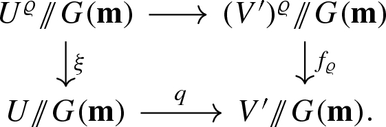
It was shown by Kaledin–Verbitsky [41] and Losev [47] that each symplectic resolution $\mathfrak {M}_{\theta }$ of the quotient singularity Y admits a universal graded Poisson deformation $\mathcal {X} \rightarrow \mathfrak {h}$, where $\mathfrak {h} = N^1(X/Y) \otimes _{\mathbb {Q}} \mathbb {C}\cong \Theta \otimes _{\mathbb {Q}} \mathbb {C}$. Namikawa [62] showed that Y also admits a universal graded Poisson deformations $\mathcal {Y} \rightarrow \mathfrak {h}/ W$. On the other hand, by taking the preimage under the moment map of a point $\lambda \in \mathfrak {h}$, one gets a graded Poisson deformation $\varvec{\mathfrak {M}}_{\theta } \rightarrow \mathfrak {h}$ for any $\theta \in \Theta$. The morphism $f_{\theta } :\mathfrak {M}_{\theta } \rightarrow \mathfrak {M}_0$ obtained by variation of GIT quotient extends to a projective morphism $\varvec{f}_{\theta } :\varvec{\mathfrak {M}}_{\theta } \rightarrow \varvec{\mathfrak {M}}_{0}$.

Theorem 1.10

Let $C\subseteq \Theta$ be a chamber, and let $\theta \in C$.

• (i) There exists a unique $w \in W$ and graded Poisson isomorphism $\varvec{\mathfrak {M}}_{\theta } {\;{\mathop {\rightarrow }\limits ^{_\sim }}\;}\mathcal {X}$ such that the diagram

  

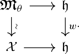
  commutes. Thus, the flat family $\varvec{\mathfrak {M}}_{\theta } \rightarrow \mathfrak {h}$ is the universal graded Poisson deformation of $\mathfrak {M}_{\theta }$.

• (ii) The morphism $\varvec{f}_{\theta } :\varvec{\mathfrak {M}}_{\theta } \rightarrow \varvec{\mathfrak {M}}_{0}$ is a crepant resolution, and an isomorphism in codimension one.

The situation is summarised in the following commutative diagram

where the lower right rectangle is shown to be Cartesian.

1.6 Relation to other work

We have chosen to state Theorem 1.7 in a manner parallel to the main result of Bayer–Macrì [5, Theorem 1.3] on moduli spaces of Bridgeland-stable objects on a projective K3 surface. On the face of it, such a link is perhaps unsurprising because X has trivial canonical class and is projective over an affine. However, it is important to note that X is not derived equivalent to the preprojective algebra $\Pi$; the stability space $\Theta$ studied here is isomorphic to the rational Picard group of X rather than the rational Grothendieck group. Put another way, the framed McKay quiver has too few vertices to be the quiver encoding a tilting bundle on X when $n>1$. In particular, the quiver varieties $\mathfrak {M}_\theta (\varvec{v},\mathbf {w})$ that we study here cannot be realised directly as moduli spaces of Bridgeland-stable objects in the derived category of coherent sheaves on X in the manner described in [4, Section 7].

Recently, McGerty–Nevins [54] have shown that Kirwan surjectivity holds for quiver varieties. That is, for each chamber C, with $\theta \in C$, the natural map $K_C :\mathbb {C}[\mathfrak {g}] = H_G^*(\mathrm {pt},\mathbb {C}) \rightarrow H^*(\mathfrak {M}_\theta (\varvec{v},\mathbf {w}),\mathbb {C})$ is surjective. Our map $L_C$ fits naturally into a commutative diagram

where $\mathbb {X}(\mathfrak {g}) \subset \mathbb {C}[\mathfrak {g}]$ is the space of characters of $\mathfrak {g}$. As noted above, it follows easily from Theorem 1.1 that $L_C$ is an isomorphism. The two vertical maps are also isomorphisms, so the map $K_C :\mathbb {X}(\mathfrak {g}) \rightarrow H^2(\mathfrak {M}_\theta (\varvec{v},\mathbf {w}),\mathbb {C})$ is an isomorphism too in our case. Therefore, our main results demonstrate precisely the extent to which the linear map $K_C$ extends across chambers to give a linear map on a union of chambers.

Since this paper was written, Theorem 1.5 enabled Gammelgaard, Gyenge, Szendrői and the second author [15] to construct the Hilbert scheme of n points on $\mathbb {C}^2/\Gamma$ as a quiver variety $\mathfrak {M}_\theta$ for a particular non-generic parameter $\theta$. Nakajima [60] subsequently used this description in his proof of the conjecture describing the generating series of Euler characteristics of ${{\,\mathrm{{\mathrm {Hilb}}}\,}}^{[n]}(\mathbb {C}^2/\Gamma )$ by Gyenge, Némethi and Szendrői [33].

2 A wall-and-chamber structure

We begin by providing an elementary description of a wall-and-chamber decomposition of a rational vector space $\Theta$, together with an action of the Namikawa Weyl group on $\Theta$. This section is purely combinatorics and uses no machinery from Geometric Invariant Theory (GIT).

2.1 The chamber decomposition

Let $\Gamma \subset \mathrm {SL}(2,\mathbb {C})$ be a finite subgroup and let $n\ge 1$ be an integer. Let V denote the given 2-dimensional representation of $\Gamma$ and list the irreducible representations as $\rho _0,\ldots , \rho _r$, where $\rho _0$ is the trivial representation.

The McKay graph is the affine Dynkin diagram associated to $\Gamma$ by the McKay correspondence; explicitly, the vertex set is $\mathrm {Irr}(\Gamma )$, and there are $\dim {{\,\mathrm{\mathrm {Hom}}\,}}_{\Gamma }(\rho _i,\rho _j\otimes V)$ edges between vertices $\rho _i$ and $\rho _j$. Since V is self-dual, this is symmetric in $\rho _i$ and $\rho _j$. Let $A_\Gamma$ denote the adjacency matrix of this graph. McKay [55] observed that if we define $C_\Gamma := 2\mathrm {Id}-A_\Gamma$ and equip the integral representation ring

$$\begin{aligned} R(\Gamma ):=\bigoplus _{0\le i\le r} \mathbb {Z}\rho _i \end{aligned}$$

with the symmetric bilinear form given by $(\alpha ,\beta )_\Gamma := \alpha ^tC_\Gamma \beta$, then we obtain the root lattice of an affine root system $\Phi _{\mathrm {aff}}$ of type ADE in which the McKay graph is the Dynkin diagram, the irreducible representations $\{\rho _0,\ldots , \rho _r\}$ provide a system of simple roots, and the regular representation

$$\begin{aligned} \delta :=\sum _{0\le i\le r} (\dim _\mathbb {C}\rho _i) \rho _i \end{aligned}$$

is the minimal imaginary root. The corresponding root system of finite type $\Phi \subset \Phi _\mathrm {aff}$ is the intersection of $\Phi _\mathrm {aff}$ with the integer span of the nontrivial irreducible representations. Let $\Phi ^+$ denote the set of positive roots.

Let $\Theta :={{\,\mathrm{\mathrm {Hom}}\,}}(R(\Gamma ),\mathbb {Q})$ denote the rational vector space whose underlying lattice is dual to $R(\Gamma )$. We adopt the following notation: write elements of $\Theta$ as $\theta =(\theta _0,\ldots ,\theta _r)\in \Theta$ where $\theta _i:=\theta (\rho _i)$ for $0\le i\le r$. Given $v\in R(\Gamma )$, we let $v^\perp := \{\theta \in \Theta \mid \theta (v)=0\}$ denote the dual hyperplane; and given $v_1,\ldots , v_m\in R(\Gamma )$, we let $\langle v_1,\ldots ,v_m\rangle ^\vee := \{\theta \in \Theta \mid \theta (v_i)\ge 0 \text { for }1\le i\le m\}$ denote the corresponding polyhedral cone.

Consider the hyperplane arrangement in $\Theta$ given by

$$\begin{aligned} \mathcal {A}= & {} \left\{ \delta ^\perp , (m\delta +\alpha )^\perp \mid \alpha \in \Phi , -n< m< n \right\} \nonumber \\= & {} \{ \delta ^\perp , (m\delta \pm \alpha )^\perp \mid \alpha \in \Phi ^+, \ 0 \le m < n \}. \end{aligned}$$

(2.1)

A chamber in $\Theta$ is the intersection with $\Theta$ of a connected component of the locus

$$\begin{aligned} \big (\Theta \otimes _{\mathbb {Q}} \mathbb {R}\big ) {\smallsetminus } \bigcup _{\gamma ^\perp \in \mathcal {A}} \gamma ^\perp . \end{aligned}$$

and we let $\Theta ^{\mathrm {reg}}$ denote the union of all chambers in $\Theta$. The closure of each chamber defines a top-dimensional cone in a chamber complex in $\Theta$ determined by $\mathcal {A}$, and the codimension-one faces of these top-dimensional cones are called walls in $\Theta$. Each wall is contained in a unique hyperplane from $\mathcal {A}$.

Example 2.1

• 1. The interior $C_-$ of the closed cone

  $$\begin{aligned} \big \langle \delta , \pm m \delta + \alpha \mid 0 \le m < n, \;\alpha \in \Phi ^+\big \rangle ^\vee \end{aligned}$$

  (2.2)

  is a chamber of $\Theta$. Indeed, since $C_-$ is cut out by specifying a strict inequality for each hyperplane in $\mathcal {A}$, the claim follows provided that we show that it’s non-empty. Let $h= \sum _{0\le i\le r} \delta _i$ be the Coxeter number of $\Phi$. If we set $\theta _i = 1$ for $i \ge 1$ and $\theta _0 = \frac{1}{2n} - h + 1$, then $\theta (m \delta ) = \frac{m}{2n}$ and $\theta (\alpha ) \ge 1$ for all $\alpha \in \Phi ^+$. This shows that $\theta \in C_-$ as required.

• 2. The interior $C_+$ of the closed cone

  $$\begin{aligned} \big \langle \delta , \alpha , m \delta \pm \alpha \mid 1 \le m < n, \alpha \in \Phi ^+ \big \rangle ^\vee \end{aligned}$$

  (2.3)

  is also a chamber in $\Theta$, because if we set $\theta _i = 1$ for $i \ge 0$, then $\theta \in C_+$ and the statement follows by the same logic as in part (1). In fact, $C_+$ can be described more simply as the interior of the cone

  $$\begin{aligned} \big \langle \rho _0,\rho _1,\ldots ,\rho _r\big \rangle ^\vee . \end{aligned}$$

  (2.4)

  Indeed, since $\theta _0 = \theta (\delta - \beta )$ where $\beta$ is the highest positive root, we have that the closure of $C_+$ is contained in (2.4). For the opposite inclusion, $m\delta > \alpha$ for $1\le m < n$, so each of $\delta , \alpha , m\delta \pm \alpha$ can be expressed as a positive sum of $\rho _0,\ldots , \rho _r$. It follows that the inequalities defining $C_+$ in (2.3) can be deduced from the inequalities $\theta _i\ge 0$ for $0\le i\le r$ which characterise the cone (2.4).

2.2 The Namikawa Weyl group

We now introduce an action of a finite group on $\Theta$. For $1\le i\le r$, let $s_i:R(\Gamma )\rightarrow R(\Gamma )$ denote reflection in the hyperplane $\{v\in R(\Gamma ) \mid (v,\rho _i)_\Gamma =0\}$ orthogonal to $\rho _i$. Explicitly, for any $0\le j\le r$, if we write $c_{i,j}$ for the (i, j)-th entry of the Cartan matrix $C_{\Gamma }$, then

$$\begin{aligned} s_i(\rho _j) = \rho _j-c_{i,j}\rho _i. \end{aligned}$$

(2.5)

In addition, consider the involution $s_\delta :R(\Gamma ) \rightarrow R(\Gamma )$ defined by sending $\delta$ to $-\delta$ and fixing $\rho _1,\ldots , \rho _r$; explicitly,

$$\begin{aligned} s_{\delta }(\rho _j) = \left\{ \begin{array}{ll} \rho _0 - 2 \delta &{}\quad \text {for}j=0, \\ \rho _j &{}\quad \text {for}1\le j\le r. \end{array}\right. \end{aligned}$$

(2.6)

We caution the reader that the subspace in $R(\Gamma )$ orthogonal (with respect to $( - , - )_{\Gamma }$) to $\rho$ differs from $\rho ^\perp = \{\theta \in \Theta \mid \theta (\rho )=0\}$, which is a hyperplane in the dual space $\Theta$.

We are primarily interested in the dual action on $\Theta$. For $1\le i\le r$, we use the same notation $s_i:\Theta \rightarrow \Theta$ for the linear map defined for $\theta \in \Theta$ and $0\le j\le r$ by setting $s_i(\theta )(\rho _j) = \theta (s_i^{-1}(\rho _j)) = \theta (s_i(\rho _j))$, where we use the fact that $s_i$ is an involution. It follows for $\theta \in \Theta$ and $1\le i\le r$ that $s_i(\theta )\in \Theta$ has components

$$\begin{aligned} s_i(\theta )_j = \theta _j - c_{i,j}\theta _i \end{aligned}$$

for all $0\le j\le r$. Note that $s_i$ is reflection in the hyperplane $\rho _i^\perp$. Similarly, the dual map $s_\delta :\Theta \rightarrow \Theta$ sends $\theta$ to the vector $s_\delta (\theta )$ with components

$$\begin{aligned} s_{\delta }(\theta )_j = \left\{ \begin{array}{ll} \theta _0 - 2 \theta (\delta ) &{}\quad \text {for }j=0, \\ \theta _j &{}\quad \text {for }1\le j\le r. \end{array}\right. \end{aligned}$$

Now define the Namikawa Weyl group to be the group

$$\begin{aligned} W:=\langle s_\delta , s_1,\ldots , s_r\rangle \end{aligned}$$

generated by these reflections of $\Theta$.

Proposition 2.2

The Namikawa Weyl group W satisfies the following properties:

• (i) it is isomorphic to $\mathfrak {S}_2 \times W_{\Gamma }$, where $W_\Gamma$ is the Weyl group of the root system $\Phi$;

• (ii) the simplicial cone in $\Theta$ defined by

  $$\begin{aligned} F:= \langle \delta ,\rho _1,\ldots ,\rho _r\rangle ^\vee \end{aligned}$$

  is a fundamental domain for the action of W on $\Theta$; and

• (iii) the action of W on $\Theta$ permutes the hyperplanes in $\mathcal {A}$ and hence permutes the set of chambers.

In particular, for every chamber C in $\Theta$, there exists a unique $w\in W$ such that $w(C)\subset F$.

Proof

For (i), change basis on $R(\Gamma )$ from $\{\rho _0,\rho _1,\ldots ,\rho _r\}$ to $\{\delta ,\rho _1,\ldots ,\rho _r\}$. The vector $\delta$ is orthogonal to the hyperplane spanned by $\rho _1,\ldots ,\rho _r$ with respect to the symmetric bilinear form on $R(\Gamma )$, so the basis $\{\delta ,\rho _1,\ldots ,\rho _r\}$ provides a set of simple roots for the decomposable root system of type $A_1\oplus \Phi$. Since $s_1,\ldots ,s_r$ generate $W_\Gamma$, it follows $s_\delta ,s_1,\ldots ,s_r$ generate the Weyl group $\mathfrak {S}_2 \times W_{\Gamma }$ of this root system and part (i) follows by changing basis back to $\{\rho _0,\rho _1,\ldots ,\rho _r\}$. For (ii), the positive orthant in the basis $\{\delta ,\rho _1,\ldots ,\rho _r\}$ provides a fundamental domain for the action of the Weyl group $\mathfrak {S}_2 \times W_{\Gamma }$. After changing basis back to $\{\rho _0,\rho _1,\ldots ,\rho _r\}$, we see that the cone F is a fundamental domain for the action of W. For (iii), the action of the generator $s_\delta$ fixes $\delta ^\perp$ and exchanges $(m\delta +\alpha )^\perp$ with $(m\delta -\alpha )^\perp$ for all $0\le m<n$ and $\alpha \in \Phi ^+$, while the simple reflections $s_1,\ldots , s_r$ permute the hyperplanes in $\mathcal {A}$. It follows that W permutes the chambers. $\square$

2.3 Counting chambers

The supporting hyperplanes of F lie in $\mathcal {A}$, so $F\cap \Theta ^\mathrm {reg}$ is a union of chambers. Our next goal is to count the number of chambers in F. We begin with a useful lemma.

Lemma 2.3

The hyperplanes of $\mathcal {A}$ passing through the interior of F are those of the form $(m\delta -\alpha )^\perp$ for $0< m< n$ and $\alpha \in \Phi ^+$.

Proof

We give two proofs. For the first, we claim that F is equal to the cone in $\Theta$ generated by the closures of the cones $C_\pm$ from Example 2.1. Indeed, the cone F is generated by the vectors $f_0,\ldots , f_r\in \Theta$ where $f_0:=(1,0,\ldots ,0)$ and, for $1\le i\le r$, the vector $f_i$ satisfies

$$\begin{aligned} f_i(\rho _j):=\left\{ \begin{array}{ll} -\dim (\rho _i) &{}\quad \text {for }j=0, \\ 1 &{}\quad \text {for }j=i, \\ 0 &{}\quad \text {otherwise}. \end{array}\right. \end{aligned}$$

We have that $f_0\in \overline{C_+}$ and $f_1,\ldots , f_r\in \overline{C_-}$, so F lies in the cone generated by $\overline{C_-}\cup \overline{C_+}$. For the opposite inclusion, we have $C_+\subset F$ by (2.4), while the inequalities $\theta (\alpha )>0$ for $\alpha \in \Phi ^+$ defining $C_-$ include $\theta (\rho _i)>0$ for $1\le i\le r$ and hence $C_-\subset F$. This proves the claim. It follows that the walls passing through the interior of F are those for which the corresponding defining inequality changes from > to < or vice-versa when we compare $C_\pm$. The result follows by comparing the lists from (2.2) and (2.3).

The second approach is more explicit. The hyperplanes $\delta ^\perp$ and $\alpha ^\perp$ for $\alpha \in \Phi ^+$ support the facets of F and can be discarded. Notice that if $\theta$ is in the interior of F then $\theta (\delta ), \theta (\alpha ) > 0$ implies that $\theta (m \delta + \alpha ) > 0$, so the hyperplanes $(m \delta + \alpha )^\perp$ for $\alpha \in \Phi ^+$ and $0<m<n$ do not intersect the interior of F. Hence it suffices to show that $(m \delta - \alpha )^\perp$ intersects the interior of F for all $0< m < n$ and $\alpha \in \Phi ^+$. Let $\theta _i= 1$ for $1\le i\le r$. Then for any choice of $\theta _0$, the parameter $\theta =(\theta _0,\ldots , \theta _r)\in \Theta$ satisfies $\theta (\gamma ) = \mathrm {ht}(\gamma )>0$ for all $\gamma \in \Phi ^+$. Now

$$\begin{aligned} \theta (m \delta - \alpha ) = m \theta _0 + m \mathrm {ht}(\beta ) - \mathrm {ht}(\alpha ), \end{aligned}$$

where $\beta \in \Phi ^+$ is the highest root (notice that $\mathrm {ht}(\beta ) = h - 1$). Set $\theta _0 = \frac{1}{m} \mathrm {ht}(\alpha ) - \mathrm {ht}(\beta )$. Then the parameter $\theta =(\theta _0,\ldots , \theta _r)\in \Theta$ satisfies

$$\begin{aligned} \theta (\delta ) = \frac{1}{m} \mathrm {ht}(\alpha ) - \mathrm {ht}(\beta ) + \mathrm {ht}(\beta ) > 0, \end{aligned}$$

so it lies in the interior of F. By construction, we have $\theta (m \delta - \alpha ) = 0$, so $\theta$ lies on the required hyperplane. $\square$

Theorem 2.4

The cone F contains precisely

$$\begin{aligned} \prod _{i=1}^{r} \frac{(n-1)h+d_i}{d_i} \end{aligned}$$

(2.7)

chambers, where r is the rank, h is the Coxeter number and $d_1,\ldots , d_r$ are the degrees of the basic polynomial invariants of $W_\Gamma$.

Proof

Every chamber in F intersects the affine hyperplane $\Lambda :=\{\theta \in \Theta \mid \theta (\delta )=1\}$ in an open region of dimension r, so it suffices to count the number of these regions. The hyperplanes $\rho _i^\perp$ for $1\le i\le r$ intersect $\Lambda$ to give a system of coordinate hyperplanes in $\Lambda \cong \mathbb {Q}^r$ with origin at $f_0 = (1,0,\ldots ,0)\in \Theta$, and $\Lambda \cap F$ is the positive orthant $\mathbb {Q}^r_{\ge 0}$. More generally, the intersection of $\Lambda$ with the hyperplanes from Lemma 2.3 and the hyperplanes $\rho _i^\perp$ for $1\le i\le r$ defines the following collection of affine hyperplanes in $\Lambda$:

$$\begin{aligned} \big \{\theta \in \Lambda \mid \theta (\beta ) = m\big \} \quad \text {for }0 \le m< n, \; \beta \in \Phi ^+; \end{aligned}$$

this is the $(n-1)$-extended Catalan hyperplane arrangement of $\Phi$ from [3], or one of the truncated $\Phi _\mathrm {aff}$-affine arrangements from [64]. It follows that the connected components of $\Lambda \cap F\cap \Theta ^{\mathrm {reg}}$ are precisely the regions in the fundamental chamber of this hyperplane arrangement. To see that the number of such regions is given by formula (2.7), substitute $d_i=e_i+1$ for $1\le i\le r$ where $e_1,\ldots ,e_r$ are the exponents of the Weyl group $W_\Gamma$ (see, for example, Carter [13, Corollary 10.2.4]), and apply Athanasiadis [3, Corollary 1.3]. $\square$

Remark 2.5

• 1. The proof of Theorem 2.4 shows that the unbounded regions in the $(n-1)$-extended Catalan hyperplane arrangement of $\Phi$ are precisely the intersection with the affine hyperplane $\Lambda$ of those chambers in F whose closure touches the facet $\delta ^\perp$ of F.

• 2. Proposition 2.2 and Theorem 2.4 together imply that there are

  $$\begin{aligned} 2\vert W_\Gamma \vert \prod _{i=1}^{r} \frac{(n-1)h+d_i}{d_i} \end{aligned}$$

  chambers in $\Theta$.

Example 2.6

For $n=4$ and $\Phi$ of type $A_2$, Fig. 1 illustrates in two ways the decomposition of the cone F into chambers: Fig. 1a shows all 22 regions in the fundamental chamber of the 3-extended Catalan hyperplane arrangement of $\Phi$ in the affine plane $\Lambda$ parallel to $\delta ^\perp$ that was introduced in the proof of Theorem 2.4; Fig. 1b shows the height-one slice of F and its division into 22 chambers. In each case, we indicate where the chambers $C_\pm$ lie. The seven unbounded regions in Fig. 1a correspond to the seven chambers in Fig. 1b whose closure touches the facet of F in $\delta ^\perp$. Notice that three chambers in F are not the interior of a simplicial cone.

Fig. 1

Chamber decomposition: a fundamental chamber; b transverse slice of F

3 Étale local normal form for quiver varieties

Modelled on Crawley-Boevey’s étale local description of affine quiver varieties, we give an étale local normal form for the morphism between quiver varieties defined by variation of GIT quotient. Pullback allows us to identify the tautological bundles on the quiver variety with the tautological bundles on the normal form. The results of this section hold for arbitrary quiver varieties.

3.1 Nakajima quiver varieties

Choose an arbitrary finite graph and let H be the set of pairs consisting of an edge, together with an orientation on it. Let ${{\,\mathrm{tl}\,}}(a)$ and ${{\,\mathrm{hd}\,}}(a)$ denote the tail and head respectively of the oriented edge $a \in H$. Let $a^*$ denote the same edge, but with opposite orientation. We fix an orientation of the graph, that is, a subset $\Omega \subset H$ such that $\Omega \cup \Omega ^* = H$ and $\Omega \cap \Omega ^* = \emptyset$. Then $\epsilon : H \rightarrow \{ \pm 1 \}$ is defined to take value 1 on $\Omega$ and $-1$ on $\Omega ^*$. Identify the vertex set of the graph with $\{ 0, 1, \dots , r \}$ for some $r\ge 1$.

Fix collections $V_0, \dots , V_r$ and $W_0, \dots , W_r$ of finite-dimensional complex vector spaces and set

$$\begin{aligned} \varvec{v}= (\dim V_0, \dots , \dim V_r), \quad \mathbf {w}= (\dim W_0, \dots , \dim W_r). \end{aligned}$$

The group $G(\varvec{v}) := \prod _{k = 0}^r {{\,\mathrm{\mathrm {GL}}\,}}(V_k)$ acts naturally on the space

$$\begin{aligned} \mathbf {M}(\varvec{v},\mathbf {w})&:= \left( \bigoplus _{a \in H} {{\,\mathrm{\mathrm {Hom}}\,}}_{\mathbb {C}}(V_{{{\,\mathrm{tl}\,}}(a)}, V_{{{\,\mathrm{hd}\,}}(a)})\right) \\&\quad \oplus \left( \bigoplus _{k = 0}^r \big ({{\,\mathrm{\mathrm {Hom}}\,}}_{\mathbb {C}}(V_k,W_k) \oplus {{\,\mathrm{\mathrm {Hom}}\,}}_{\mathbb {C}}(W_k,V_k)\big )\right) . \end{aligned}$$

This action of $G(\varvec{v})$ is Hamiltonian for the natural symplectic structure on $\mathbf {M}(\varvec{v},\mathbf {w})$ and, after identifying the dual of $\mathfrak {g}(\varvec{v}) := \mathrm {Lie} \ G(\varvec{v})$ with $\mathfrak {g}(\varvec{v})$ via the trace pairing, the corresponding moment map ${\mu } :\mathbf {M}(\varvec{v},\mathbf {w}) \rightarrow \mathfrak {g}(\varvec{v})$ satisfies

$$\begin{aligned} {\mu }(B,i,j) = \left( \sum _{{{\,\mathrm{hd}\,}}(a) = k} \epsilon (a) B_a B_{a^*} + i_k j_k \right) _{k = 0}^r \end{aligned}$$

where $i_k \in {{\,\mathrm{\mathrm {Hom}}\,}}_{\mathbb {C}}(W_k,V_k), j_k \in {{\,\mathrm{\mathrm {Hom}}\,}}_{\mathbb {C}}(V_k,W_k)$ and $B_a \in {{\,\mathrm{\mathrm {Hom}}\,}}_{\mathbb {C}}(V_{{{\,\mathrm{tl}\,}}(a)},V_{{{\,\mathrm{hd}\,}}(a)})$. Though one can talk about arbitrary stability conditions in this context, as was done in [59], it is easier in our case to apply the trick of Crawley-Boevey [19] and reduce to the case where each $W_k = 0$ by introducing a framing vertex.

The set H associated to the graph can be thought of as the arrow set of a quiver. We frame this quiver by adding an additional vertex $\infty$, as well as $\mathbf {w}_i$ arrows from vertex $\infty$ to vertex i and another $\mathbf {w}_i$ arrows from vertex i to vertex $\infty$. This framed (doubled) quiver is denoted $Q = (I,Q_1)$, where $I = \{ \infty , 0, \dots , r \}$. Each dimension vector $\varvec{v}= (\dim V_0, \dots , \dim V_r)$ for the original graph determines a dimension vector for Q that we write (without bold font) as $v = (1,\dim V_0, \dots , \dim V_r)$. We may identify $\mathbf {M}(\varvec{v},\mathbf {w})$ with the space

$$\begin{aligned} {{\,\mathrm{\mathrm {Rep}}\,}}(Q,v):= \bigoplus _{a\in Q_1} {{\,\mathrm{\mathrm {Hom}}\,}}_{\mathbb {C}}(\mathbb {C}^{{{\,\mathrm{tl}\,}}(a)},\mathbb {C}^{{{\,\mathrm{hd}\,}}(a)}) \end{aligned}$$

of representations of Q of dimension vector v in such a way that the $G(\varvec{v})$-action on $\mathbf {M}(\varvec{v},\mathbf {w})$ corresponds to the action of the group $G(v):=\big (\prod _{i\in I} {{\,\mathrm{\mathrm {GL}}\,}}(v_i)\big )/\mathbb {C}^\times$ on ${{\,\mathrm{\mathrm {Rep}}\,}}(Q,v)$ by conjugation and, moreover, that the above map ${\mu }$ corresponds to the moment map $\mu$ induced by this G(v)-action on ${{\,\mathrm{\mathrm {Rep}}\,}}(Q,v)$. If we write

$$\begin{aligned} \Theta _{v}:= \big \{\theta \in {{\,\mathrm{\mathrm {Hom}}\,}}(\mathbb {Z}^I,\mathbb {Q}) \mid \theta (v)=0\big \}, \end{aligned}$$

then every character of G(v) is of the form $\chi _\theta :G(v)\rightarrow \mathbb {C}^\times$ for some integer-valued $\theta \in \Theta _{v}$, where $\chi _\theta (g) = \prod _{i \in I} \det (g_i)^{\theta _i}$ for $g\in G(v)$. For $\theta \in \Theta _v$, after replacing $\theta$ by a positive multiple if necessary, the (Nakajima) quiver variety associated to $\theta$ is the categorical quotient

$$\begin{aligned} \mathfrak {M}_\theta (\varvec{v},\mathbf {w}) := \mu ^{-1}(0)/\,/_{\chi _\theta } G(v)= \mu ^{-1}(0)^{\theta }/\,/G(v) = {{\,\mathrm{\mathrm {Proj}}\,}}\bigoplus _{k\ge 0} \mathbb {C}[\mu ^{-1}(0)]^{\chi _{k\theta }}, \end{aligned}$$

where $\mu ^{-1}(0)^{\theta }$ denotes the locus of $\chi _\theta$-semistable points in $\mu ^{-1}(0)$ and $\mathbb {C}[\mu ^{-1}(0)]^{\chi _{k\theta }}$ is the $\chi _{k\theta }$-semi-invariant slice of the coordinate ring of the affine variety $\mu ^{-1}(0)$. Note that $\mathbb {C}^\times$ acts on $\mathbf {M}(\varvec{v},\mathbf {w})$ by scaling, and this action descends to an action on $\mathfrak {M}_\theta (\varvec{v},\mathbf {w})$.

For a more algebraic description of $\mathfrak {M}_\theta (\varvec{v},\mathbf {w})$, extend $\epsilon$ to Q by setting $\epsilon (a) = 1$ if $a :\infty \rightarrow i$ and $\epsilon (a) = -1$ if $a :i \rightarrow \infty$. The preprojective algebra $\Pi$ is the quotient of the path algebra $\mathbb {C}Q$ by the relation

$$\begin{aligned} \sum _{a \in Q_1} \epsilon (a) aa^* = 0. \end{aligned}$$

(3.1)

Given $\theta \in \Theta _v$, we say that a $\Pi$-module M of dimension vector v is $\theta$-semistable if $\theta (N)\ge 0$ for all submodules $N\subseteq M$, and it is $\theta$-stable if $\theta (N)>0$ for all proper nonzero submodules. A finite dimensional $\Pi$-module is said to be $\theta$-polystable if it is a direct sum of $\theta$-stable $\Pi$-modules. King [42] proved that a $\Pi$-module M of dimension vector v is $\theta$-semistable (resp. $\theta$-stable) if and only if the corresponding point of $\mu ^{-1}(0)$ is $\chi _\theta$-semistable (resp. $\chi _\theta$-stable) in the sense of GIT. In fact [42, Propositions 3.2,5.2] establishes that the quiver variety $\mathfrak {M}_\theta (\varvec{v},\mathbf {w})$ is the coarse moduli space of ${{\,\mathrm{\mathrm {S}}\,}}$-equivalence classes of $\theta$-semistable $\Pi$-modules of dimension vector v, where the closed points of $\mathfrak {M}_\theta (\varvec{v},\mathbf {w})$ are in bijection with the $\theta$-polystable representations of $\Pi$ of dimension v. The (possibly empty) open subset of $\mathfrak {M}_\theta (\varvec{v},\mathbf {w})$ parameterizing $\theta$-stable representations will be denoted $\mathfrak {M}_\theta (\varvec{v},\mathbf {w})^s$.

The geometry of the quiver varieties $\mathfrak {M}_\theta (\varvec{v},\mathbf {w})$ may change as we vary the stability parameter $\theta \in \Theta _v$. We say that $\theta \in \Theta _v$ is effective (with respect to v) if there exists a $\theta$-semistable $\Pi$-module of dimension vector v, and it is generic (with respect to v) if every $\theta$-semistable $\Pi$-module of dimension vector v is $\theta$-stable. The work of Dolgachev–Hu [23] and Thaddeus [65] implies that there is a wall-and-chamber structure on the cone of effective stability parameters in $\Theta _v$, where two generic parameters $\theta , \theta ^\prime \in \Theta _v$ lie in the same (open) GIT chamber if and only if the notions of $\theta$-stability and $\theta ^\prime$-stability coincide, in which case $\mathfrak {M}_\theta (\varvec{v},\mathbf {w})\cong \mathfrak {M}_{\theta ^\prime }(\varvec{v},\mathbf {w})$. The GIT walls of a GIT chamber are the codimension-one faces of the closure of the chamber.

Remark 3.1

Note that a priori, the locus of generic stability parameters could be empty.

3.2 A local normal form

We begin by describing an étale local form for $\mathfrak {M}_{\theta }(\varvec{v},\mathbf {w})$ based on Luna’s slice theorem, generalising [21, Section 4]. Let A be the adjacency matrix of the framed (doubled) quiver Q, i.e.

$$\begin{aligned} A = (a_{i,j}), \quad a_{i,j} := | \{ a \in Q_1 \ | \ {{\,\mathrm{tl}\,}}(a) = i, {{\,\mathrm{hd}\,}}(a) = j \}|. \end{aligned}$$

Then A is a symmetric matrix and we define a symmetric bilinear form on $\mathbb {Z}^I$ by setting

$$\begin{aligned} (\alpha ,\beta ) := \alpha ^t C \beta \end{aligned}$$

where $C = 2 \mathrm {Id} - A$ is the Cartan matrix of Q. Let p be the quadratic form on $\mathbb {Z}^{I}$ defined by setting

$$\begin{aligned} p(\alpha ) = 1 - \frac{1}{2}(\alpha ,\alpha ). \end{aligned}$$

Let $\theta \in \Theta _v$, and choose $\theta _0 \in \Theta _v$ that lies in the boundary of the closure of the GIT chamber containing $\theta$ (the stability condition $\theta _0$ should not be confused with the component of $\theta$ corresponding to the vertex 0; in all that follows, we never refer to the latter). Then there is a projective morphism

$$\begin{aligned} f :\mathfrak {M}_{\theta }(\varvec{v},\mathbf {w}) \rightarrow \mathfrak {M}_{\theta _0}(\varvec{v},\mathbf {w}) \end{aligned}$$

induced by variation of GIT quotient. In this generality, f need not be birational.

Choose a closed point $x \in \mathfrak {M}_{\theta _0}(\varvec{v},\mathbf {w})$ and write $M_{\infty } \oplus M_0^{\mathbf {m}_0} \oplus \cdots \oplus M_k^{\mathbf {m}_k}$ for the corresponding $\theta _0$-polystable representation, where $M_{\infty }$ is the unique $\theta _0$-stable summand with $(\dim M_{i})_{\infty } \ne 0$. For $0\le i\le k$, let $\beta ^{(i)}\in \mathbb {Z}^I$ denote the dimension vector of $M_i$. Following Nakajima [56, Section 6] and Crawley-Boevey [21, Section 4], define the ${{\,\mathrm{\mathrm {Ext}}\,}}$-graph associated to x to be the graph with vertex set $\{ 0, \dots , k \}$, and edge set comprising $p(\beta ^{(i)})$ loops at vertex i and $-(\beta ^{(i)}, \beta ^{(j)})$ edges between i and j; the terminology is motivated by [18, Lemma 1]. Note that the ${{\,\mathrm{\mathrm {Ext}}\,}}$-graph is empty if and only if x is a $\theta _0$-stable point, see Remark 3.3. We form new dimension vectors

$$\begin{aligned} \mathbf {m}= (\mathbf {m}_0, \dots , \mathbf {m}_k) \quad \text { and }\quad \mathbf {n}= (\mathbf {n}_0, \dots , \mathbf {n}_k), \end{aligned}$$

(3.2)

where $\mathbf {n}_i = - (\beta ^{(\infty )},\beta ^{(i)})$. Finally, define the exponent $\varrho \in {{\,\mathrm{\mathrm {Hom}}\,}}(\mathbb {Z}^{k+1},\mathbb {Q})$ for a rational character of $G(\mathbf {m})$ by

$$\begin{aligned} \varrho (\gamma ) = \theta \left( \sum _{i = 0}^k \gamma _i \beta ^{(i)}\right) \end{aligned}$$

(3.3)

for $\gamma = (\gamma _i)\in \mathbb {Z}^{k+1}$. The corresponding character of $G(\mathbf {m})$ is obtained from the character $\chi _\theta$ of $G(\varvec{v})$ by restriction, i.e., $\chi _\varrho = {{\,\mathrm{{\mathrm {res}}}\,}}^{G(\varvec{v})}_{G(\mathbf {m})}(\chi _\theta )$. We write $f_{\varrho } :\mathfrak {M}_{\varrho }(\mathbf {m},\mathbf {n}) \rightarrow \mathfrak {M}_{0}(\mathbf {m},\mathbf {n})$ for the projective morphism.

Theorem 3.2

Let $\ell = p(\beta ^{(\infty )}) \ge 0$. There exist affine open neighbourhoods $V \subset \mathfrak {M}_{\theta _0}(\varvec{v},\mathbf {w})$ and $V^{\prime } \subset \mathfrak {M}_0(\mathbf {m},\mathbf {n}) \times \mathbb {C}^{2\ell }$ of x and 0 respectively, together with a projective morphism $\xi :\overline{Z}\rightarrow Z$ and a closed point $z\in Z$, forming a diagram

where both squares are Cartesian, all horizontal maps are étale, and where $p(z)=x$, $q(z)=0$.

Remark 3.3

If the point x is $\theta _0$-stable, then the ${{\,\mathrm{\mathrm {Ext}}\,}}$-graph is empty, the quiver variety $\mathfrak {M}_0(\mathbf {m},\mathbf {n})$ is a closed point, and $\ell =p(\varvec{v}) = \frac{1}{2}\dim \mathfrak {M}_{\theta _0}(\varvec{v},\mathbf {w})$.

Theorem 3.2 implies:

Corollary 3.4

There is an isomorphism $f^{-1}(x) \cong (f_{\varrho }\times \mathrm {id})^{-1}(0)$. In particular,

• (i) $f^{-1}(x) \ne \emptyset$ if and only if $(f_{\varrho }\times \mathrm {id})^{-1}(0) \ne \emptyset$; and

• (ii) $\dim f^{-1}(x) = \dim \; (f_{\varrho }\times \mathrm {id})^{-1}(0)$.

Passing to the formal neighbourhood of x in V, and the formal neighbourhood of $f^{-1}(x)$ in $f^{-1}(V)$, we deduce, as was explained in [8, Section 2.1.6], that there is a commutative diagram of formal schemes:

3.3 The proof of Theorem 3.2

Choose a lift $y \in \mu ^{-1}(0)^{\theta _0}$ of x whose $G(\varvec{v})$-orbit is closed in $\mu ^{-1}(0)^{\theta _0}$. As shown in [7, Lemma 3.2], the stabiliser subgroup $G(\varvec{v})_y\cong G(\mathbf {m})$ is a reductive subgroup of $G(\varvec{v})$. Since $G(\mathbf {m})$ is reductive, it is explained in [21, Section 4] that one can find a coisotropic $G(\mathbf {m})$-module complement C to $\mathfrak {g}(\varvec{v})\cdot y$ in $\mathbf {M}(\varvec{v},\mathbf {w})$. As in loc. cit., we let $\mu _y$ denote the composition of $\mu$ with the quotient map $\mathfrak {g}(\varvec{v})^* \rightarrow \mathfrak {g}(\mathbf {m})^*$ and let L be a $G(\mathbf {m})$-stable complement to $\mathfrak {g}(\mathbf {m})$ in $\mathfrak {g}(\varvec{v})$. As in loc. cit., we define $\nu :C \rightarrow L^*$ by

$$\begin{aligned} \nu (c)(l) = \omega (c,ly) + \omega (c,lc) + \omega (y,lc), \end{aligned}$$

where $\omega$ is the G-invariant symplectic form on $\mathbf {M}(\varvec{v},\mathbf {w})$. For $c\in C$, $g\in \mathfrak {g}(\mathbf {m})$ and $l\in L$ we calculate

$$\begin{aligned} \mu (y+c)(g+l) = \omega \big (y+c,(g+l)(y+c)\big ) = \nu (c)(l) + \mu _y(c)(g). \end{aligned}$$

(3.6)

The following two results are each a relative version of [7, Theorem 3.3].

Lemma 3.5

There exists a $G(\mathbf {m})$-saturated affine open subset $U_0$ of $0 \in C$ such that:

• (i) the map from $U := U_0 \cap \mu _y^{-1}(0) \cap \nu ^{-1}(0)$ to $\mu ^{-1}(0)^{\theta _0}$ sending c to $y+c$ induces an étale morphism

  $$\begin{aligned} p :G(\varvec{v}) \times _{G(\mathbf {m})} U \rightarrow \mu ^{-1}(0)^{\theta _0} \end{aligned}$$

  whose image V is a $G(\varvec{v})$-saturated affine open subset of $\mu ^{-1}(0)^{\theta _0}$;

• (ii) the map p restricts to an étale map $G(\varvec{v}) \times _{G(\mathbf {m})} U^{\varrho } \rightarrow V^{\theta }$ sending the point (1, 0) to y; and

• (iii) these maps induce a Cartesian diagram

  

  with both horizontal maps étale.

Proof

Equation (3.6) shows that if $c\in \mu _y^{-1}(0)\cap \nu ^{-1}(0)$ then $y+c\in \mu ^{-1}(0)$. We now apply [7, Equation (4), Lemma 3.9] to obtain a $G(\mathbf {m})$-saturated affine open neighbourhood $U_0$ of 0 in C such that (i) holds.

For (ii), it suffices to show that $p^{-1}(V^{\theta }) = G(\varvec{v}) \times _{G(\mathbf {m})} U^{\varrho }$. To show that the left hand side is contained in the right hand side, we need only show that if $c \in U$ such that $y + c \in V^{\theta }$, then $c \in U^{\varrho }$. If $y + c \in V^{\theta }$ then there exists an $m \theta$-semi-invariant function $\gamma$ on V such that $\gamma (y + c) \ne 0$. Define $h:C \rightarrow \mathbb {C}$ by setting $h(c) = \gamma (y + c)$. Then h is $\varrho$-semi-invariant, and hence $c \in U^{\varrho }$. For the opposite inclusion, the tensor product of the counit and the identity map gives a $G(\mathbf {m})$-module homomorphism $\mathbb {C}[G(\varvec{v}) \times _{G(\mathbf {m})} U]\rightarrow \mathbb {C}[U]$, and Frobenius reciprocity [38, Proposition 3.4] gives

$$\begin{aligned} \mathbb {C}[G(\varvec{v}) \times _{G(\mathbf {m})} U]^{\chi _\theta }&\cong {{\,\mathrm{\mathrm {Hom}}\,}}_{G(\varvec{v})}\big (\chi _\theta ,\mathbb {C}[G(\varvec{v}) \times _{G(\mathbf {m})} U]\big )\\&\cong {{\,\mathrm{\mathrm {Hom}}\,}}_{G(\mathbf {m})}\big ({{\,\mathrm{{\mathrm {res}}}\,}}^{G(\varvec{v})}_{G(\mathbf {m})} (\chi _\theta ),\mathbb {C}[U]\big )\cong \mathbb {C}[U]^{\chi _{\varrho }}. \end{aligned}$$

If $c \in U^{\varrho }$ then choose $h \in \mathbb {C}[U]^{k\varrho }$ for some $k>0$ such that $h(c) \ne 0$. We define $h' \in \mathbb {C}[G(\varvec{v}) \times _{G(\mathbf {m})} U]^{\chi _{k\theta }}$ by $h'(g,c) = \chi _\theta (g) h(c)$. Now,

$$\begin{aligned} G(\varvec{v}) \times _{G(\mathbf {m})} U \cong V \times _{V/\,/ G(\varvec{v})} U/\,/ G(\mathbf {m}) \end{aligned}$$

and hence $\mathbb {C}[G(\varvec{v}) \times _{G(\mathbf {m})} U] \cong \mathbb {C}[V] \otimes _{\mathbb {C}[V]^{G(\varvec{v})}} \mathbb {C}[U]^{G(\mathbf {m})}$. Thus, there exist $h_i \in \mathbb {C}[V]^{\chi _{k\theta }}$ and $\gamma _i \in \mathbb {C}[U]^{G(\mathbf {m})}$ such that $h' = \sum _i h_i \otimes \gamma _i$. In particular,

$$\begin{aligned} h(c) = h'(1,c) = \sum _i h_i(y + c) \gamma _i(\overline{c}) \ne 0 \end{aligned}$$

implies that there is some $h_i \in \mathbb {C}[V]^{\chi _{k\theta }}$ such that $h_i(y + c) \ne 0$. In particular, $y + c \in V^{\theta }$, so (ii) holds.

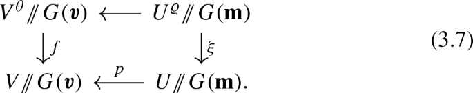
This also implies that that diagram

is Cartesian, with the horizontal maps being étale and $G(\varvec{v})$-equivariant. Taking the GIT quotient gives the Cartesian diagram (3.7), so (iii) holds as required. $\square$

Let $\mu _{\mathbf {m}}$ denote the moment map for the action of $G(\mathbf {m})$ on $\mathbf {M}(\mathbf {m},\mathbf {n})$. It is explained in [21, Section 4] that $C\cap (\mathfrak {g}(\varvec{v}) \cdot y)^\perp$ can be identified, as a $G(\mathbf {m})$-module, with representations of a certain doubled quiver. This doubled quiver is precisely the framed doubled quiver associated to the ${{\,\mathrm{\mathrm {Ext}}\,}}$-graph described in Sect. 3.2, except that we have neglected to include the $p(\beta ^{(\infty )}) = \ell$ loops at vertex $\infty$ in our ${{\,\mathrm{\mathrm {Ext}}\,}}$-graph. Since the dimension vector m of the framed doubled quiver satisfies $m_{\infty } = 1$, there is a factor of $\mathbb {C}^{2 \ell }$ in the representation space, corresponding to the value of the endomorphisms at the loops, on which $G(\mathbf {m})$ acts trivially. That is, we can identify $C\cap (\mathfrak {g}(\varvec{v}) \cdot y)^\perp = \mathbf {M}(\mathbf {m},\mathbf {n}) \times \mathbb {C}^{2 \ell }$ as $G(\mathbf {m})$-modules, where $G(\mathbf {m})$ acts trivially on $\mathbb {C}^{2 \ell }$, in such a way that $\mu _{\mathbf {m}}$ is identified with the restriction of $\mu _y$ to $C \cap (\mathfrak {g}(\varvec{v}) \cdot y)^\perp$.

Lemma 3.6

There exists a $G(\mathbf {m})$-saturated affine open subset U of $0 \in \mu _y^{-1}(0) \cap \nu ^{-1}(0)$ such that:

• (i) the projection $q:U \rightarrow \mu _{\mathbf {m}}^{-1}(0) \times \mathbb {C}^{2 \ell }$ is étale with image W a $G(\mathbf {m})$-saturated affine open subset;

• (ii) q restricts to an étale map $U^{\varrho } \rightarrow (V^{\prime })^{\varrho }$ sending 0 to 0; and

• (iii) these maps induce a Cartesian diagram

  

  with both horizontal maps étale.

Proof

The proof of the lemma is a straight-forward (but easier) adaptation of the proof of [21, Lemma 4.8], as in the proof of Lemma 3.5. $\square$

Theorem 3.2 follows directly from the following more precise statement.

Theorem 3.7

There exists an affine $G(\mathbf {m})$-variety U, and an affine open $G(\varvec{v})$-stable subset $V \subset \mu ^{-1}(0)^{\theta _0}$ containing y and an affine open $G(\mathbf {m})$-stable subset $V^{\prime } \subset \mu _{\mathbf {m}}^{-1}(0) \times \mathbb {C}^{2 \ell }$ containing 0, forming a diagram

where both squares are Cartesian, all horizontal maps are étale, and where the class of a closed point $u\in U$ has image under p and q equal to x and 0 respectively.

Proof

The required properties of diagram (3.8) follow from Lemmas 3.5 and 3.6 since, taking their intersection if necessary, we may assume that the two affine sets U of the lemmata are equal. Note that the image of the class of $u:=0\in U$ under p and q is the class of y and the class of 0 respectively. $\square$

3.4 Tautological bundles

Tautological bundles play a key role in understanding the birational transformations that occur as one crosses the walls in the space $\Theta _v$ of GIT stability conditions. We now describe what happens to the tautological bundles under the morphisms of Theorem 3.2.

Recall that Q is a doubled quiver with framing vertex $\infty$, and v denotes the dimension vector for Q associated to a dimension vector $\varvec{v}$ for $Q {\smallsetminus } \{ \infty \}$. Since v is primitive, King [42, Proposition 5.3] proves that for generic $\theta \in \Theta _v$, the quiver variety $\mathfrak {M}_\theta (\varvec{v},\mathbf {w})=\mu ^{-1}(0)^{\theta } /\,/\ {G(v)}$ is the fine moduli space of isomorphism classes of $\theta$-stable $\Pi$-modules of dimension vector v. In this case, the universal family on $\mathfrak {M}_\theta (\varvec{v},\mathbf {w})$ is a tautological locally-free sheaf

$$\begin{aligned} \mathcal {R}:=\mathcal {R}_\theta (\varvec{v},\mathbf {w}) \cong \bigoplus _{i\in I} \mathcal {R}_i \end{aligned}$$

where $\text {rank} \,(\mathcal {R}_i)=v_i$ for $i\in I$, together with a $\mathbb {C}$-algebra homomorphism $\Pi \rightarrow {{\,\mathrm{\mathrm {End}}\,}}(\mathcal {R})$. Explicitly, for $i \in I$ we write $F_i$ for the representation of G(v) obtained by pulling back the vectorial representation from the ith factor of G(v). Then $\mathcal {R}_i$ is the locally-free sheaf associated to the vector bundle

$$\begin{aligned} \mu ^{-1}(0)^{\theta } \times _{G(v)} F_i \rightarrow \mu ^{-1}(0)^{\theta } /\,/\ {G(v)} = \mathfrak {M}_{\theta }(\varvec{v},\mathbf {w}). \end{aligned}$$

When we wish to emphasise the dependence of $\mathcal {R}_i$ on the dimension vectors, we write $\mathcal {R}_i(\varvec{v},\mathbf {w})$. Since $\mathcal {R}$ is defined only up to tensor product by an invertible sheaf, we normalise by fixing $\mathcal {R}_\infty$ to be the trivial bundle.

As in Sect. 3.2, choosing a closed point $x\in \mathfrak {M}_{\theta _0}(\varvec{v},\mathbf {w})$, where $\theta _0$ lies in the closure of the GIT chamber containing $\theta$, determines $k\ge 0$ and dimension vectors $\beta ^{(0)},\ldots , \beta ^{(k)}\in \mathbb {Z}^{I}$, dimension vectors $\mathbf {m}, \mathbf {n}$ for the Ext-graph of x, and a stability condition $\varrho \in {{\,\mathrm{\mathrm {Hom}}\,}}(\mathbb {Z}^{k+1},\mathbb {Q})$, which determine the quiver variety $\mathfrak {M}_\varrho (\mathbf {m},\mathbf {n})$. Recall now the statement of Theorem 3.2, and specifically, diagram (3.4):

Proposition 3.8

The quiver variety $\mathfrak {M}_\varrho (\mathbf {m},\mathbf {n})$ carries a tautological locally-free sheaf $\bigoplus _{j} \mathcal {R}_j(\mathbf {m},\mathbf {n})$, where j ranges over the set $\{\infty ,0,\ldots ,k\}$. Moreover, for each $i\in I{\setminus } \{\infty \}$, there is an isomorphism of bundles on $Z'$ given by

$$\begin{aligned} p_{\theta }^* \ \mathcal {R}_i(\varvec{v},\mathbf {w}) \cong \bigoplus _{j = 0}^k q_{\varrho }^*\ \mathcal {R}_j(\mathbf {m},\mathbf {n})^{\oplus \beta _i^{(j)}}. \end{aligned}$$

Proof

The vector $\mathbf {m}$ determines a dimension vector m for the framed (doubled) quiver satisfying $m_\infty =1$, so m is primitive. In light of [42, Proposition 5.3], it remains to show that $\varrho$ is generic in order to prove the first statement.

We claim that if $\theta$ is generic with respect to v then $\varrho$ is generic with respect to m. Our argument is based on the proof of [46, Proposition 1.1]. Assume that $\varrho$ is not generic for m. Then the locus of strictly polystable representations in $\mathfrak {M}_\varrho (\mathbf {m},\mathbf {n})$ is non-empty. The scaling action of $\mathbb {C}^{\times }$ on $\mathfrak {M}_0(\mathbf {m},\mathbf {n})$ defined in Sect. 3.1 lifts to $\mathfrak {M}_\varrho (\mathbf {m},\mathbf {n})$, and the locus of strictly polystable representations is both closed and $\mathbb {C}^{\times }$-stable. Hence, there exists a strictly polystable point r in $f_{\varrho }^{-1}(0)$. Choose a lift $(r',0)$ of (r, 0) in $W^{\varrho } \subseteq \mu ^{-1}_{\mathbf {m}}(0) \times \mathbb {C}^{2 \ell }$ whose $G(\mathbf {m})$-orbit is closed. The fact that the diagram (3.8) is Cartesian means that there is a point $z' \in \xi ^{-1}(z)$ mapping to (r, 0). Let $x'$ be the image of this point in $V^{\theta }/\,/G(\varvec{v})$. If $y'$ is a lift of $x'$ in $V^{\theta }$, whose $G(\varvec{v})$-orbit is closed then the final statement of [49, Theoreme du slice étale] implies that $G(\varvec{v})_{y'} \cong G(\mathbf {m})_{(r',0)} = G(\mathbf {m})_{r'}$. The fact that r is strictly polystable means that $G(\mathbf {m})_{r'}$, and hence $G(\varvec{v})_{y'}$, is non-trivial. This in turn implies that $x'$ is strictly polystable, contradicting the assumption that $\theta$ is generic for v.

For the second statement, the locally-free sheaf $p_{\theta }^* \mathcal {R}_i(\varvec{v},\mathbf {w})$ is the sheaf of sections of the map

$$\begin{aligned} (V^{\theta } \times _{G(\varvec{v})} F_i) \times _{V^{\theta } /\,/\ G(\varvec{v})} U^{\varrho } /\,/\ G(\mathbf {m})&\cong (G(\varvec{v}) \times _{G(\mathbf {m})} U^{\varrho }) \times _{G(\varvec{v})} F_i \\&\cong U^{\varrho } \times _{G(\mathbf {m})} F_i \longrightarrow U^{\varrho } /\,/\ G(\mathbf {m}); \end{aligned}$$

here the first isomorphism follows from the proof of Lemma 3.5, and the second is a consequence of Luna’s slice theorem [49]. Similarly, $q_{\varrho }^* \mathcal {R}_j(\mathbf {m},\mathbf {n})$ corresponds to sections of $U^{\varrho } \times _{G(\mathbf {m})} F_j(\mathbf {m},\mathbf {n}) \rightarrow U^{\varrho } /\,/\ G(\mathbf {m},\mathbf {n})$. Thus, the result follows from the fact that

$$\begin{aligned} F_i |_{G(\mathbf {m})} \cong \bigoplus _{j = 0}^k F_j(\mathbf {m},\mathbf {n})^{\oplus \beta _i^{(j)}}. \end{aligned}$$

This latter decomposition is simply the fact that x corresponds to the $\theta _0$-polystable representation

$$\begin{aligned}&M_{\infty } \oplus M_0^{\oplus \mathbf {m}_0} \oplus \cdots \oplus M_k^{\oplus \mathbf {m}_{k}} \\&= M_{\infty } \oplus \big (M_0 \otimes F_1(\mathbf {m},\mathbf {n})\big ) \oplus \cdots \oplus \big (M_k \otimes F_k(\mathbf {m},\mathbf {n})\big ). \end{aligned}$$

This completes the proof. $\square$

3.5 A stratification

There are two natural ways of defining a finite stratification of the quiver variety. The first is Luna’s stratification, coming from the fact that it is a GIT quotient by a reductive group. The second is the stratification into symplectic leaves, which is finite since the quiver variety has symplectic singularities [7, Theorem 1.2]. It is known that these two stratifications agree [7, Proposition 3.6]. In this section, we recall the definition of these strata. In order to do so, we first recall Crawley-Boevey’s canonical decomposition of a dimension vector.

As explained in [39], associated to the Cartan matrix C of the framed (doubled) quiver $Q=(I,Q_1)$ is a root system $R \subset \mathbb {Z}^I$, with positive roots $R^+ = R \cap \mathbb {Z}^I_{\ge 0}$. For $\theta \in {{\,\mathrm{\mathrm {Hom}}\,}}(\mathbb {Z}^{I},\mathbb {Q})$, set $R_{\theta }^+ = \{ \alpha \in R^+ \mid \theta (\alpha ) = 0 \}$ and define

$$\begin{aligned} \Sigma _{\theta }= & {} \left\{ \alpha \in R^+_{\theta } \ \Big | \ p(\alpha )> \sum _{i = 0}^k p\left( \beta ^{(i)}\right) , \ \forall \ \alpha = \beta ^{(0)} + \cdots + \beta ^{(k)},\right. \nonumber \\&\qquad \qquad \left. k > 0, \beta ^{(i)} \in R^+_{\theta } \right\} . \end{aligned}$$

(3.10)

In general, it is very difficult to compute $\Sigma _{\theta }$, but notice that if $\theta (\beta ) \ne 0$ for all roots $\beta < \alpha$, then $\alpha \in \Sigma _{\theta }$.

Theorem 3.9

• (i) For $v\in \mathbb {N}^{I}$, there exists a $\theta$-stable $\Pi$-module of dimension vector v iff $v \in \Sigma _{\theta }$.

• (ii) Let $\mathbb {N}R_{\theta }^+$ denote the subsemigroup of $\mathbb {N}^{I}$ generated by $R_{\theta }^+$. Each $v \in \mathbb {N}R_{\theta }^+$ admits a decomposition

  $$\begin{aligned} v = \gamma ^{(0)} + \cdots + \gamma ^{(\ell )}, \end{aligned}$$

  (3.11)

  where $\gamma ^{(i)} \in \Sigma _{\theta }$ for $0\le i\le \ell$, such that any other decomposition of v as a sum of elements from $\Sigma _\theta$ is a refinement of the sum (3.11); this is the canonical decomposition of v with respect to $\theta$.

• (iii) The canonical decomposition (3.11) is characterised by the fact that

  $$\begin{aligned} \sum _{i = 0}^{\ell } p\left( \gamma ^{(i)}\right) > \sum _{j = 0}^{k} p\left( \beta ^{(j)}\right) \end{aligned}$$

  for any other decomposition $v = \beta ^{(0)} + \cdots + \beta ^{(k)}$ of v with each $\beta ^{(i)} \in \Sigma _{\theta }$.

• (iv) For $v\in \mathbb {N}R_{\theta }^+$ as in (3.11), let M be a generic $\theta$-polystable $\Pi$-module of dimension v with decomposition $M=M_0^{\oplus m_0}\oplus \dots \oplus M_{\ell }^{\oplus m_{\ell }}$ into pairwise non-isomorphic $\theta$-stable representations. Then, grouping like terms together $v = m_1 \xi ^{(1)} + \cdots + m_{\ell } \xi ^{(\ell )}$ in the canonical decomposition (3.11), we have $\dim M_i = \xi ^{(i)}$.

Proof

This is due to Crawley-Boevey [19, 20], but see Bellamy–Schedler [7] in this generality. In particular, property (iii) can be deduced from [20, Corollary 1.4]. $\square$

The strata of $\mathfrak {M}_{\theta }(\varvec{v},\mathbf {w})$ are labelled by the “representation types” of v, which we now recall. A representation type $\tau$ of v is a tuple

$$\begin{aligned} \tau = (n_0,\beta ^{(0)}; \dots ; n_{k}, \beta ^{(k)}) \end{aligned}$$

where $\beta ^{(i)} \in \Sigma _{\theta }$, $n_i \in \mathbb {Z}_{> 0}$ and $\sum _{i = 0}^k n_i \beta ^{(i)} = v$. The stratum labelled by the representation type $\tau$ is:

$$\begin{aligned} \mathfrak {M}_{\theta }(\varvec{v},\mathbf {w})_{\tau }&:= \left\{ M_0^{\oplus n_0} \oplus \cdots \oplus M_{k}^{\oplus n_{k}} \in \mathfrak {M}_{\theta _0}(\varvec{v},\mathbf {w}) \right. \\&\qquad \qquad \left. | \ M_i \text { is } \theta \text {-stable and } \dim M_i = \beta ^{(i)} \right\} . \end{aligned}$$

Remark 3.10

By [7, Corollary 3.25], each stratum is a connected locally-closed, smooth subvariety of $\mathfrak {M}_{\theta }(\varvec{v},\mathbf {w})$. Since the dimension of the locus of $\theta$-stable points in $\mathfrak {M}_{\theta }(\varvec{v},\mathbf {w})$ equals 2p(v), Theorem 3.9(i) implies that the stratum $\mathfrak {M}_{\theta }(\varvec{v},\mathbf {w})_{\tau }$ is non-empty if and only if $\beta ^{(i)} \ne \beta ^{(j)}$ when $\beta ^{(i)}$ and $\beta ^{(j)}$ are real roots. The stratification is finite, and

$$\begin{aligned} \dim \mathfrak {M}_{\theta }(\varvec{v},\mathbf {w})_{\tau } = 2 \sum _{i = 0}^{k} p\left( \beta ^{(i)}\right) . \end{aligned}$$

See [7, Section 3.5] and references therein for more information.

4 Quiver varieties for the framed McKay quiver

We now specialise to the case where the quiver varieties $\mathfrak {M}_\theta (\varvec{v},\mathbf {w})$ are constructed from the affine Dynkin diagram associated to $\Gamma$ by the McKay correspondence.

4.1 Canonical decomposition of roots

Once and for all, we fix the graph to be the McKay graph of $\Gamma \subset \mathrm {SL}(2,\mathbb {C})$ and fix dimension vectors $\varvec{v}:= n \delta$ and $\mathbf {w}= \rho _0$, so that the corresponding framed, doubled quiver Q is the framed McKay quiver, with vertex set $I = \{\rho _\infty ,\rho _0,\rho _1,\ldots ,\rho _r\}$. The dimension vector for representations of Q is

$$\begin{aligned} v:= \rho _{\infty } + n \delta \in \mathbb {Z}^{I}. \end{aligned}$$

Define

$$\begin{aligned} \Theta _v:= \{\theta \in {{\,\mathrm{\mathrm {Hom}}\,}}(\mathbb {Z}^{I},\mathbb {Q}) \mid \theta (v)=0\}, \end{aligned}$$

and write elements of $\Theta _{v}$ as $\theta =(\theta _\infty ,\theta _0,\ldots ,\theta _r)$ where $\theta _i:=\theta (\rho _i)$ for $i\in \{\infty ,0,1,\ldots ,r\}$. For $\theta \in \Theta _v$, set

$$\begin{aligned} \mathfrak {M}_\theta := \mathfrak {M}_\theta (\varvec{v},\mathbf {w}) = \mathfrak {M}_{\theta }(Q,v). \end{aligned}$$

(4.1)

As explained in Sect. 3.5, associated to the quiver Q is the root system $R \subset \mathbb {Z}^I$, and $R^+=\mathbb {N}^{I}\cap R$ the set of positive roots. We can recover the affine root system $\Phi _\mathrm {aff}$ associated to $\Gamma$ in Sect. 2.1 as follows.

Lemma 4.1

We have $\Phi _\mathrm {aff}= \{ \alpha = (\alpha _i)_{i\in I} \in R \mid \alpha _{\infty } = 0 \}$

Proof

The fact that $\Phi _\mathrm {aff}$ is contained in the right-hand side follows from the fact that the adjacency matrix $A_\Gamma$ of the McKay graph is obtained by deleting the row and column indexed by $\rho _\infty$ from the adjacency matrix A for Q. For the opposite inclusion, suppose $\alpha =(\alpha _\infty ,\alpha _0,\ldots ,\alpha _r)\in R^+$ satisfies $\alpha _\infty =0$. Since $\alpha$ is a positive root, we have $(\alpha ,\alpha )\le 2$. If we set $\alpha ^\prime :=(\alpha _0,\ldots ,\alpha _r)\in R(\Gamma )$, then $\alpha _\infty =0$ gives $(\alpha ^\prime ,\alpha ^\prime )_\Gamma =(\alpha ,\alpha )\le 2$ and hence the fact that $A_{\Gamma }$ is positive semi-definite implies, by [39, Proposition 5.10], that $\alpha \in \Phi _\mathrm {aff}^+$. It follows that the set $\{\alpha \in R \mid \alpha _\infty =0\}$ is contained in $\Phi _\mathrm {aff}$. $\square$

Lemma 4.1 enables us to identify the root lattice $\mathbb {Z}^{I}$ with the lattice $\mathbb {Z}\oplus R(\Gamma )$, with the standard basis corresponding to $\{\rho _\infty , \rho _0,\rho _1,\ldots ,\rho _r\}$.

Our next goal is to prove the following result about the canonical decomposition of v (see Theorem 3.9 for the definition).

Proposition 4.2

Let $\theta \in \Theta _{v}$. Then $v\in R_\theta ^+$. Moreover:

• (i) if $\theta _\infty \ne 0$ then the canonical decomposition of v with respect to $\theta$ is v; and

• (ii) if $\theta _\infty = 0$ then the canonical decomposition is $v = \rho _{\infty } + \delta + \cdots + \delta$, where $\delta$ appears n times here.

The proof requires two preliminary results, the first of which is an application of the Frenkel–Kac theorem.

Lemma 4.3

If $\gamma =(\gamma _i)_{i\in I} \in R^+$ satisfies $\gamma _{\infty } = 1$, then there exists $\nu \in \bigoplus _{i\ge 1} \mathbb {Z}\rho _i$ such that

$$\begin{aligned} \gamma = \rho _{\infty } + m \delta + \frac{1}{2} (\nu ,\nu ) \delta - \nu , \end{aligned}$$

(4.2)

where $m=p(\gamma )$. Conversely, any vector of this form lies in $R^+$.

Proof

Let $V(\omega _0)$ be the vacuum module (of level one) for the Kac–Moody algebra with root system R. The Frenkel–Kac theorem [39, Lemma 12.6] says that w is a weight of $V(\omega _0)$ if and only if

$$\begin{aligned} w = \omega _0 - m \delta - \frac{1}{2} (\nu ,\nu ) \delta + \nu , \end{aligned}$$

for some $\nu \in \bigoplus _{i\ge 1} \mathbb {Z}\rho _i$ and $m \ge 0$. Then, the statement follows from [59, Lemma 2.14]. $\square$

Lemma 4.4

For $\theta \in \Theta _{v}$, we have $v\in R_\theta ^+$ and $p(v) = n$. In particular, if $n > 1$ then v is an anisotropic root.

Proof

Lemma 4.3 implies that $v\in R_\theta ^+$. For $i > 0$, we have $(\rho _i,\rho _{\infty } + n \delta ) = 0$. We compute $(\rho _0, \rho _{\infty } + n \delta ) = (\rho _0, \rho _{\infty }) = -1$ and $(\rho _{\infty }, \rho _{\infty } + n \delta ) = 2 - n$, giving $p(v) = n$. Therefore, if $n > 1$, then v belongs to the fundamental domain of Q and $p(v) > 1$. This means that v is an anisotropic root. $\square$

Proof of Proposition 4.2

Lemma 4.4 gives $v \in R_{\theta }^+$, so we obtain a canonical decomposition

$$\begin{aligned} v= \gamma ^{(0)} + \cdots + \gamma ^{(\ell )} \end{aligned}$$

by Theorem 3.9. We may assume that $\gamma ^{(0)}_{\infty } = 1$.

Suppose first that $\theta _\infty =0$, so that $\theta (\delta ) = 0$. Then the fact that $p(s \delta ) = 1$ for all $s \ge 1$ implies that the only multiple of $\delta$ in $\Sigma _{\theta }$ is $\delta$ itself. Similarly, the decomposition

$$\begin{aligned} (\rho _{\infty } + m \delta ) = \rho _{\infty } + \delta + \cdots + \delta \end{aligned}$$

implies that $\rho _{\infty } + m \delta \notin \Sigma _{\theta }$ for any $m > 0$ because $m = p(\rho _{\infty } + m \delta ) = p(\rho _{\infty }) + p(\delta ) + \cdots + p(\delta )$ would contradict the inequality in (3.10). In particular, $v \notin \Sigma _{\theta }$. Therefore the canonical decomposition of v has $\ell \ge 1$. Let $\gamma ^{(1)}, \dots , \gamma ^{(k)}$ be all roots in the expression that equal $\delta$ (for some $1 \le k \le n$). By Lemma 4.3, the root $\gamma ^{(0)}$ is of the form (4.2) for some $m \le n - \ell$ and $\nu \in \oplus _{i \ge 1} \mathbb {Z}\rho _i$. Each $\gamma ^{(i)}$ for $i > k$ is a real root in $(\Phi _\mathrm {aff})^+_{\theta } := \{ v \in \Phi _\mathrm {aff}^+ \mid \theta (v) = 0 \}$. In particular, $\sum _i p\left( \gamma ^{(i)}\right) = m + k$. By definition of $\Sigma _{\theta }$ and the characterisation of canonical decomposition given in Theorem 3.9(iii), we must have

$$\begin{aligned} n = p(v) \le \sum _i p\left( \gamma ^{(i)}\right) = m + k; \end{aligned}$$

otherwise $v \in \Sigma _{\theta }$, which we have shown is not true. Therefore, we deduce that $n = m + k$. This implies that $(\nu ,\nu ) = 0$. Since $( - , - )$ is positive definite on $\bigoplus _{i \ge 1} \mathbb {Z}\rho _i$, this means that $\nu = 0$, forcing $\gamma ^{(0)} = \rho _{\infty } + m \delta$. But we have shown above that this in turn forces $m = 0$ because $\gamma ^{(0)} \in \Sigma _{\theta }$. Hence $k = n$, implying that the canonical decomposition of v is $\rho _{\infty } + \delta + \cdots + \delta$.

If $\theta _{\infty } \ne 0$ then none of the roots $\gamma ^{(i)}$ is a multiple of $\delta$. Hence every $\gamma ^{(i)}$, for $i > 0$, is a real root in $(\Phi _\mathrm {aff})^+_{\theta }$. Again assuming that $\gamma ^{(0)}$ has the form given in (4.2) for some $m \le n$, this implies by Theorem 3.9(iii) that $\sum _i p\left( \gamma ^{(i)}\right) = p\left( \gamma ^{(0)}\right) = m \ge n$. Therefore, we must have $m = n$, and $(\nu ,\nu ) = 0$. Once again, since $( - , - )$ is positive definite on $\bigoplus _{i \ge 1} \mathbb {Z}\rho _i$, this means that $\nu = 0$, and hence $v \in \Sigma _{\theta }$ has trivial canonical decomposition. $\square$

4.2 Characterising smooth quiver varieties

The following description of the affine quotient corresponding to the stability parameter $\theta =0$ is well-known.

Lemma 4.5

There is an isomorphism of algebraic varieties $\mathfrak {M}_0\cong \mathbb {C}^{2n} / \Gamma _n$ that is also an isomorphism of Poisson varieties (up to rescaling the bracket by some $t \in \mathbb {C}^{\times }$).

Proof

This follows from results of Crawley-Boevey [20]; see also Kuznetsov [45, Proposition 33]. Indeed, Proposition 4.2 shows that the canonical decomposition of v in $\Sigma _0$ is $\rho _{\infty } + \delta + \cdots + \delta$, where $\delta$ appears n times in the sum. If $\mathfrak {M}^{\mathrm {pt}}_0(\varvec{v},\mathbf {w})$ denotes a quiver variety associated to the graph with a single vertex and no edges, and $\mathfrak {M}^{\mathrm {Mc}}_0(\varvec{v},\mathbf {w})$ a quiver variety associated to the unframed McKay quiver, then Crawley-Boevey’s canonical decomposition (see also [19, Lemma 9.2]) implies that

$$\begin{aligned} \mathfrak {M}_0 \cong \mathfrak {M}^{\mathrm {pt}}_0(1,0) \times \mathrm {Sym}^n \left( \mathfrak {M}^{\mathrm {Mc}}_0(\delta ,0)\right) \end{aligned}$$

because $\rho _{\infty }$ is real and hence $p(\rho _{\infty }) = 0$. The quiver variety $\mathfrak {M}^{\mathrm {pt}}_0(1,0)$ is of course just a point, and the isomorphism $\mathfrak {M}^{\mathrm {Mc}}_0(\delta ,0) \cong \mathbb {C}^2 / \Gamma$ is due to Kronheimer [44]. The description of $\mathfrak {M}_0$ as an algebraic variety follows from the isomorphism $\mathrm {Sym}^n(\mathbb {C}^2 / \Gamma ) \cong \mathbb {C}^{2n} / \Gamma _n$. For the final statement, both varieties have a natural Poisson structure making them symplectic varieties, i.e. they have a Poisson bracket that is generically non-degenerate. Moreover, in both cases this bracket is homogeneous of degree $-2$. Any such structure on $\mathbb {C}^{2n} / \Gamma _n$ is unique up to rescaling [25, Lemma 2.23]. $\square$

To state the main result of this section, identify the space $\Theta _{v}$ of GIT stability parameters with $\Theta$ via the projection away from the $\theta _\infty$ coordinate. We obtain from (2.1) a hyperplane arrangement in $\Theta _{v}$ given by

$$\begin{aligned} \mathcal {A}_{v} = \{ \delta ^\perp , (m\delta \pm \alpha )^\perp \mid \alpha \in \Phi ^+, \ 0 \le m < n \}, \end{aligned}$$

(4.3)

where now each $\gamma \in \mathbb {Z}^I = \mathbb {Z}\oplus R(\Gamma )$ defines the dual hyperplane $\gamma ^\perp := \{\theta \in \Theta _{v} \mid \theta (\gamma )=0\}$. As before, a chamber in $\Theta _{v}$ is the intersection with $\Theta _v$ of a connected component of the locus

$$\begin{aligned} \big (\Theta _{v}\otimes _{\mathbb {Q}} \mathbb {R}\big ) {\smallsetminus } \bigcup _{\gamma ^\perp \in \mathcal {A}_{v}} \gamma ^{\perp }, \end{aligned}$$

(4.4)

and we let $\Theta _v^{\mathrm {reg}}$ denote the union of all chambers in $\Theta _v$. A wall is a codimension-one face of the closure of a chamber. A vector $w \in \Sigma _{\theta }$ is said to be minimal (with respect to $\theta$) if it does not admit a proper decomposition $w = \beta ^{(0)} + \cdots + \beta ^{(k)}$ with $k > 0$ and $\beta ^{(i)} \in \Sigma _{\theta }$.

Theorem 4.6

For $n>1$, the following conditions on a stability parameter $\theta \in \Theta _{v}$ are equivalent:

• (i) the variety $\mathfrak {M}_\theta$ is smooth;

• (ii) the canonical decomposition of v with respect to $\theta$ is of the form $\sigma ^{(0)} + \cdots + \sigma ^{(\ell )}$ where each $\sigma ^{(i)}\in \Sigma _\theta$ is minimal and a given imaginary root can appear at most once as a summand;

• (iii) the parameter $\theta$ lies in $\Theta _{v}^{\mathrm {reg}}$;

• (iv) the parameter $\theta$ is generic, i.e. every $\theta$-semistable $\Pi$-module of dimension vector v is $\theta$-stable.

Proof

Statements (i) and (ii) are equivalent by [7, Corollary 1.17]. To show that (ii) and (iii) are equivalent, assume first that $\theta \in \Theta ^{\mathrm {reg}}_{v}$. Since $\delta ^\perp = \rho _{\infty }^\perp = \{\theta \mid \theta _{\infty }=0\}$ is a wall, the canonical decomposition of v is v by Proposition 4.2. Assume that v is not minimal, i.e. it admits a proper decomposition $v = \beta ^{(0)} + \cdots + \beta ^{(k)}$ with $k > 0$ and $\beta ^{(i)} \in \Sigma _{\theta }$. Then, without loss of generality $\beta ^{(0)}_{\infty } = 1$. Hence $\beta ^{(i)} \in \Phi _\mathrm {aff}^+$ for $i > 0$. In particular, there exists some $\beta \in E := \{ \beta \in \Phi _\mathrm {aff}^+ \mid 0 < \beta \le n \delta \}$ such that $\theta (\beta ) = 0$; explicitly,

$$\begin{aligned} E= & {} \{ m \delta + \alpha \ | \ 0 \le m< n, \ \alpha \in \Phi ^{+} \} \cup \{ m \delta - \alpha \ | \ 0 < m \le n , \ \alpha \in \Phi ^+ \}\\&\cup \{ m \delta \ | \ 1 \le m \le n \}. \end{aligned}$$

The equations $\theta (\beta ) = 0$ define the hyperplanes in $\mathcal {A}_{v}$, contradicting the assumption $\theta \in \Theta ^{\mathrm {reg}}_{v}$, except in the case $n \delta - \alpha \in E$ for $\alpha \in \Phi ^+$. Suppose v admits a decomposition with some $\beta ^{(i)} = n \delta - \alpha$, for $\alpha \in \Phi ^+$. Then $\rho _{\infty } + \alpha \in \mathbb {N}\Sigma _{\theta }$, and hence $\rho _{\infty } \in \Sigma _{\theta }$ because the support of any root is connected; see for instance [39, Section 5.3]. This implies that $\theta _{\infty } = 0$, so $\theta \in \delta ^\perp$ which contradicts $\theta \in \Theta ^{\mathrm {reg}}_{v}$. Therefore v is minimal, so statement (ii) holds. Conversely, suppose that $\theta \not \in \Theta ^{\mathrm {reg}}_{v}$, i.e. $\theta$ lies in a hyperplane from $\mathcal {A}_{v}$. First, if $\theta \in \delta ^\perp = \rho _\infty ^\perp$, then $\theta _{\infty } = 0$, so the canonical decomposition of v is $\rho _{\infty }+\delta + \cdots + \delta$ by Proposition 4.2. Since $\delta$ is imaginary and $n > 1$, condition (ii) fails to hold. Next, if $\theta \in (m\delta +\alpha )^\perp$ satisfies $\theta _{\infty } \ne 0$ for some $-n< m < n$ and $\alpha \in \Phi$, then the canonical decomposition of v is v by Proposition 4.2. We claim that $v \in \Sigma _{\theta }$ is not minimal. If $m > 0$ then set $\gamma := m \delta + \alpha \in \Phi _\mathrm {aff}^+$, and if $m < 0$ then set $\gamma := - (m \delta + \alpha ) \in \Phi _\mathrm {aff}^+$. Either way, $v - \gamma$ can be expressed as a vector of the form (4.2) and hence $v-\gamma \in R^+$. In fact $v-\gamma \in R_\theta ^+$ because $\theta \in (m\delta +\alpha )^\perp =\gamma ^\perp$ gives $\theta (v-\gamma )= \pm \theta (m\delta +\alpha ) = 0$. Then both $\gamma$ and $v-\gamma$ admit a canonical decomposition by Theorem 3.9(ii), so v admits a proper decomposition. This shows that (ii) fails to hold, so (ii) and (iii) are equivalent.

For the equivalence of (iii) and (iv), the previous paragraph shows that if $\theta$ lies on any of the hyperplanes in $\mathcal {A}_{v}$, then either v admits a canonical decomposition with more than one term (i.e., the generic polystable $\Pi$-module of dimension vector v is not $\theta$-stable), or v admits a proper decomposition. Grouping like terms, such a decomposition defines a representation type $\tau$ consisting of more than one term. This implies that there are $\theta$-semistable representations of dimension v that are not $\theta$-stable. Therefore (iv) implies (iii). Conversely, if $\theta$ does not lie on a hyperplane in $\mathcal {A}_{v}$, then the previous paragraph shows that the only decomposition of v as a sum of elements from $\Sigma _{\theta }$ is v itself. Therefore every $\theta$-semistable representation is $\theta$-stable. $\square$

Remark 4.7

• 1. Theorem 4.6 implies that the wall-and-chamber structure on $\Theta _{v}$ determined by $\mathcal {A}_{v}$ coincides with the wall-and-chamber structure arising from the GIT construction of the quiver varieties $\mathfrak {M}_\theta$ for $\theta \in \Theta _{v}$. In particular, all results of Sect. 2 hold for the GIT decomposition of $\Theta _{v}$, so the walls and chambers introduced there are GIT walls and GIT chambers.

• 2. It follows from Proposition 4.2 that whenever the equivalent conditions of Theorem 4.6 hold, the canonical decomposition of v is v, and moreover v is minimal.

4.3 Crepant resolutions

We now investigate how the quiver varieties $\mathfrak {M}_\theta$ are related to each other.

Proposition 4.8

For any $\theta \in \Theta _{v}$, the morphism to the affine quotient $f_\theta :\mathfrak {M}_\theta \rightarrow \mathfrak {M}_0$ obtained by variation of GIT quotient is projective and birational. If $\theta \in \Theta ^{\mathrm {reg}}_{v}$ then $f_\theta$ is a crepant resolution.

Proof

The morphism $f_{\theta }$ is projective by construction. Moreover, as noted in Theorem A.1, $f_{\theta }$ is a Poisson morphism, birational onto its image. By Proposition 4.2, $\dim \mathfrak {M}_\theta = \dim \mathfrak {M}_0 = 2n$ and hence the image of $f_{\theta }$ is in fact $\mathfrak {M}_0$, Thus, $f_{\theta }$ is birational. Finally, if we assume that $\theta \in \Theta ^{\mathrm {reg}}_{v}$, then Theorem 4.6 says that $\mathfrak {M}_{\theta }$ is a smooth symplectic variety. This implies that $f_{\theta }$ is a symplectic, and hence crepant, resolution. $\square$

Two of the resolutions from Proposition 4.8 are well-known. For the first, let $f_S:S\rightarrow \mathbb {C}^2/\Gamma$ denote the minimal resolution. Since S is smooth, Fogarty [26] shows the Hilbert scheme of n-points on S, denoted

$$\begin{aligned} X:= {{\,\mathrm{{\mathrm {Hilb}}}\,}}^{[n]}(S), \end{aligned}$$

is smooth, and the Hilbert–Chow morphism ${{\,\mathrm{{\mathrm {Hilb}}}\,}}^{[n]}(S)\rightarrow \mathrm {Sym}^n(S)$ is a crepant resolution. By composing this with the functorial morphism $\mathrm {Sym}^n(S)\rightarrow \mathrm {Sym}^n(\mathbb {C}^2/\Gamma )$, we obtain a crepant resolution of singularities

$$\begin{aligned} f:X\longrightarrow Y:= \mathrm {Sym}^n(\mathbb {C}^2/\Gamma )\cong \mathbb {C}^{2n}/\Gamma _n, \end{aligned}$$

(4.5)

where the wreath product $\Gamma _n:=\mathfrak {S}_n \wr \Gamma = \mathfrak {S}_n \ltimes \Gamma ^n$ acts on $(\mathbb {C}^2)^n\cong \mathbb {C}^{2n}$ in the natural way. That f is an example of one of the morphisms from Proposition 4.8 is due to Kuznetsov [45]; the same observation was made independently by Haiman [34] and Nakajima [57]. To state the result, Remark 4.7 enables us to regard the chamber $C_-$ from Example 2.1(1) as a GIT chamber in $\Theta _{\varvec{v}}$.

Theorem 4.9

(Kuznetsov). For any $\theta \in C_-$, there is a commutative diagram

in which the horizontal arrows are isomorphisms and the vertical arrows are symplectic resolutions.

Proof

Kuznetsov [45, Theorem 43] gives the horizontal isomorphism $X\rightarrow \mathfrak {M}_\theta$ for stability parameters $\theta$ in an open subset of $C_-$. Since $C_-$ is a GIT chamber, the isomorphism exists for all $\theta \in C_-$. The lower horizontal isomorphism from the diagram is from Lemma 4.5, and the vertical arrows are the symplectic resolutions from (4.5) and Proposition 4.8. The diagram commutes by [45, Proof of Proposition 44]. $\square$

For the second well-known example of the morphism from Proposition 4.8, set $N:= \vert \Gamma \vert$. The action of $\Gamma$ on $\mathbb {C}^2$ induces an action of $\Gamma$ on the Hilbert scheme ${{\,\mathrm{{\mathrm {Hilb}}}\,}}^{[nN]}(\mathbb {C}^2)$. Let $n\Gamma \text {-}{{\,\mathrm{{\mathrm {Hilb}}}\,}}(\mathbb {C}^2)$ denote the subscheme parametrising $\Gamma$-invariant ideals I in ${{\,\mathrm{{\mathrm {Hilb}}}\,}}^{[nN]}(\mathbb {C}^2)$ such that the quotient $\mathbb {C}[x,y]/I$ is isomorphic to the direct sum of n copies of the regular representation of $\Gamma$. Recall the chamber $C_+$ from Example 2.1(2).

Theorem 4.10

(Varagnolo–Vasserot, Wang). For any $\theta \in C_+$, there is a commutative diagram

in which the horizontal arrows are isomorphisms and the vertical arrows are symplectic resolutions.

Proof

The isomorphism given by the top horizontal arrow is due to Varagnolo–Vasserot [66] and Wang [67, Theorem 2], while commutativity of the diagram is noted in [45, Remark 41]. $\square$

Remark 4.11

The moduli space $\mathfrak {M}_\theta$ defined by any parameter $\theta \in C_+$ is characterised among the moduli $\mathfrak {M}_\theta$ for arbitrary $\theta \in \Theta _{\varvec{v}}$ by the property that the tautological vector bundles $\mathcal {R}_i$ for $i\in I$ on $\mathfrak {M}_\theta$ are all globally generated, see [17, Corollary 2.4].

4.4 The case $n = 1$

This case is somewhat different since the quiver variety $\mathfrak {M}_\theta$ can be smooth even for non-generic parameters.

Lemma 4.12

If $n = 1$, then $\mathfrak {M}_\theta$ is smooth if and only if $\theta$ does not lie on any $\alpha ^{\perp }$, for $\alpha \in \Phi$.

Proof

The proof is identical to the proof of Theorem 4.6, except in this case when $\theta _{\infty } = 0$, the minimal imaginary root $\delta$ only appears with multiplicity one in the canonical decomposition. Therefore, a parameter $\theta$ on the hyperplane $\delta ^{\perp }$, which is not contained in any $\alpha ^{\perp }$ for $\alpha \in \Phi$, is such that $\mathfrak {M}_\theta$ is smooth. Every point of $\mathfrak {M}_{\theta }$ corresponds to a strictly polystable representation even though the moduli space is smooth. $\square$

In particular, when $n=1$ we recover the chamber structure for the unframed McKay quiver moduli construction due to Kronheimer [44] (see also Cassens–Slodowy [14]) in the hyperplane $\delta ^\perp$. Indeed, it is well-known that the chamber decomposition in this case is the Weyl chamber decomposition for $\Phi$.

4.5 Universal Poisson deformations

The description of the Namikawa Weyl group in Sect. 2.2 allows us to identify the space $\Theta _v \otimes _{\mathbb {Q}} \mathbb {C}$ with the (complex) reflection representation $\mathfrak {h}$ of W. For $\theta \in \Theta _v$, consider the family

$$\begin{aligned} \sigma _{\theta }:\varvec{\mathfrak {M}}_{\theta } := \mu ^{-1}(\mathfrak {h})^{\theta } /\,/\, G(v)\longrightarrow \mathfrak {h}\end{aligned}$$

deforming $\mathfrak {M}_{\theta }$. This becomes a graded Poisson morphism if we regard $\mathfrak {h}$ as a Poisson variety with trivial bracket. We now explain how to identify this family, when $\theta$ is generic, with the universal graded Poisson deformation of $\mathfrak {M}_{\theta }$ whose existence was shown by Kaledin–Verbitsky [41] in the ungraded case, and adapted by Losev [47] to the graded case.

There is a commutative diagram

where $\varvec{f}_{\theta } :\varvec{\mathfrak {M}}_{\theta } \rightarrow \varvec{\mathfrak {M}}_0$ is the morphism given by variation of GIT.

Lemma 4.13

The morphism $\varvec{f}_{\theta }$ is projective, birational and Poisson.

Proof

The fact that the morphism is projective and Poisson follows directly from the definition of variation of GIT. To see that it is birational it suffices to note that there is a finite collection of hyperplanes in $\mathfrak {h}$ such that $\varvec{f}_{\theta }$ is an isomorphism away from those hyperplanes. Indeed, let S denote the complement to all hyperplanes $\alpha ^{\perp }$ for $\alpha < v$ a positive root; these define proper hyperplanes in $\mathfrak {h}$ because v is indivisible. If $\lambda \in S$ then the only positive root $\alpha \le v$ in the set $\Sigma _{\lambda }$ is v itself. By [19, Theorem 1.2], this implies that every representation of the deformed preprojective algebra $\Pi ^{\lambda }$ of dimension v is simple, and hence $\theta$-stable. Thus, the restriction of $\varvec{f}_{\theta }$ to $\sigma _{\theta }^{-1}(S)$ is the identity map $\sigma _{\theta }^{-1}(S) \rightarrow \sigma _0^{-1}(S)$ because $\mu ^{-1}(S)^{\theta } = \mu ^{-1}(S)$. In particular, $\varvec{f}_{\theta }$ is birational. $\square$

Lemma 4.14

• (i) The morphism $\sigma _0$ is flat, and $\varvec{\mathfrak {M}}_0$ is irreducible, normal, and Cohen–Macaulay.

• (ii) If $\theta \in \Theta _v^{\mathrm {reg}}$, then $\sigma _\theta$ is flat and $\varvec{\mathfrak {M}}_{\theta }$ is smooth and connected.

Proof

For (i), the locus $\mu ^{-1}(\mathfrak {h})$ is cut out by $n^2 |\Gamma | - r$ equations in the affine space $\mathbf {M}(\varvec{v},\mathbf {w})$ of dimension $2n (n |\Gamma | + 1)$, so it is a complete intersection of dimension $n^2 |\Gamma | + 2n + r$ by [30, Theorem 3.7]. In particular, $\mu ^{-1}(\mathfrak {h})$ is Cohen–Macaulay, and hence the map $\mu ^{-1}(\mathfrak {h}) \rightarrow \mathfrak {h}$ is flat [53, Corollary 23.1]. Since $\mathbb {C}[\mu ^{-1}(\mathfrak {h})]^{G(v)}$ is a direct summand of $\mathbb {C}[\mu ^{-1}(\mathfrak {h})]$ as a $\mathbb {C}[\mathfrak {h}]$-module, it follows that $\sigma _0 :\varvec{\mathfrak {M}}_0 \rightarrow \mathfrak {h}$ is also flat. As for $\varvec{\mathfrak {M}}_0$, each fiber of $\sigma _0$ has symplectic singularities by [7, Theorem 1.2], so the fibres have rational singularities and hence are Cohen–Macaulay. It follows from [53, Corollary 23.3] that $\varvec{\mathfrak {M}}_0$ is Cohen–Macaulay. To show normality, it suffices to show that $\varvec{\mathfrak {M}}_0$ satisfies $(R_1)$. Let U be the set of points x in $\varvec{\mathfrak {M}}_0$ such that x is a regular point in the fiber $\sigma ^{-1}_0(\sigma _0(x))$. Then [53, Theorem 23.7] says that U is contained in the smooth locus of $\varvec{\mathfrak {M}}_0$. Thus, we need to show that the complement C to U in $\varvec{\mathfrak {M}}_0$ has codimension at least two. The image of C in $\mathfrak {h}$ is contained in the finitely many hyperplanes described in the proof of Lemma 4.13 since the set S described there satisfies $\sigma _0^{-1}(S) \subset U$. Since $C \cap \sigma _0^{-1}(\lambda )$ has codimension at least one in $\sigma _0^{-1}(\lambda )$ (in fact it has codimension at least two since each fiber $\sigma _0^{-1}(\lambda )$ is normal), $\mathrm {codim}_{\varvec{\mathfrak {M}}_0} \, C \ge \mathrm {codim}_{\mathfrak {h}} \, \sigma _0(C) + 1 \ge 2$.

For (ii), an argument similar to that for $\sigma _0$ above shows that $\sigma _{\theta }$ is also flat. As for the variety $\varvec{\mathfrak {M}}_\theta$, all maps appearing in diagram (4.6) are equivariant for the natural scaling action of $\mathbb {C}^{\times }$ described in Sect. 3.1, if we make $\mathbb {C}^{\times }$ act on $\mathfrak {h}$ with weight one. This implies that the singular locus of $\varvec{\mathfrak {M}}_{\theta }$ is a $\mathbb {C}^{\times }$-stable closed subvariety. In particular, if it is non-empty then it would intersect the zero fiber $\sigma _{\theta }^{-1}(0) = \mathfrak {M}_{\theta }$ non-trivially. However, since $\sigma _{\theta }$ is flat and $\mathfrak {M}_{\theta }$, $\mathfrak {h}$ are smooth, [53, Theorem 23.7] says that this intersection is trivial. Thus, $\varvec{\mathfrak {M}}_{\theta }$ is smooth. Similarly, each connected component of $\varvec{\mathfrak {M}}_{\theta }$ is a closed $\mathbb {C}^{\times }$-stable subvariety, and hence must intersect $\mathfrak {M}_{\theta }$ non-trivially. But the latter is irreducible, so $\varvec{\mathfrak {M}}_{\theta }$ is connected. $\square$

Proposition 4.15

The morphism $\varvec{f}_{\theta }$ is crepant, and an isomorphism in codimension one.

Proof

Let $2n = \dim \mathfrak {M}_{\theta }$. As in the proof of Lemma 4.14(ii), we note that all maps appearing in diagram (4.6) are equivariant for the natural scaling action of $\mathbb {C}^{\times }$. The Poisson bracket on both $\varvec{\mathfrak {M}}_{\theta }$ and $\varvec{\mathfrak {M}}_{0}$ is $\mathcal {O}_{\mathfrak {h}}$-linear. Since the bracket is homogeneous of degree $-2$, it defines a $\mathbb {C}^{\times }$-equivariant map $\phi _{\theta } :\Omega ^1_{\varvec{\mathfrak {M}}_{\theta }/ \mathfrak {h}} \rightarrow \mathcal {T}_{\varvec{\mathfrak {M}}_{\theta } / \mathfrak {h}} \langle 2\rangle$, where $\mathcal {T}_{\varvec{\mathfrak {M}}_{\theta } / \mathfrak {h}}$ is the sheaf of $\mathcal {O}_{\mathfrak {h}}$-linear derivations on $\varvec{\mathfrak {M}}_{\theta }$, and $\langle 2\rangle$ denotes a shift in the grading by two. The degeneracy locus of $\phi _{\theta }$ is closed and $\mathbb {C}^{\times }$-stable. In particular, if it were non-empty it would intersect the fiber $\sigma _{\theta }^{-1}(0) = \mathfrak {M}_{\theta }$ non-trivially. However, if $i : \mathfrak {M}_{\theta } \hookrightarrow \varvec{\mathfrak {M}}_{\theta }$ is the embedding of the zero fibre, then $i^* \phi _{\theta } :\Omega ^1_{\mathfrak {M}_{\theta }} \rightarrow \mathcal {T}_{\mathfrak {M}_{\theta }}$ is an isomorphism since the Poisson bracket restricted to $\mathfrak {M}_{\theta }$ is non-degenerate. Therefore, we deduce that $\phi _{\theta }$ is an isomorphism. Thus, there is a relative symplectic form $\omega _{\varvec{\mathfrak {M}}_{\theta }/ \mathfrak {h}}$ on $\varvec{\mathfrak {M}}_{\theta }$, dual to the Poisson bracket. Since $\mathfrak {h}$ is obviously smooth, this implies that $\sigma _{\theta }$ is smooth and, if $\omega _{\mathfrak {h}}$ is a nowhere vanishing top form on $\mathfrak {h}$, then $\omega _{\varvec{\mathfrak {M}}_{\theta }/ \mathfrak {h}}^n \wedge \sigma _{\theta }^* \omega _{\mathfrak {h}}$ is a nowhere vanishing top form on $\varvec{\mathfrak {M}}_{\theta }$. In particular, the canonical divisor $K_{\varvec{\mathfrak {M}}_{\theta }}$ is trivial.

Similarly, on $\varvec{\mathfrak {M}}_{0}$, we have $\phi _0 :\Omega ^1_{\varvec{\mathfrak {M}}_{0}/ \mathfrak {h}} \rightarrow \mathcal {T}_{\varvec{\mathfrak {M}}_{0}/ \mathfrak {h}}\langle 2\rangle$. Let $D \subset \varvec{\mathfrak {M}}_{0}$ be its degeneracy locus. This is a closed, $\mathbb {C}^{\times }$-stable subset of $\varvec{\mathfrak {M}}_{0}$. Let $D_{\le i} = \{ x \in D \ | \ \dim (D \cap \sigma _0^{-1}(\sigma _0(x))) \le i \}$. Then, by Chevalley’s Theorem, each $D_{\le i}$ is closed and $\mathbb {C}^{\times }$-stable. We know that $\dim D \cap \sigma ^{-1}_0(0) \le 2n -2$ since the map $\Omega ^1_{\mathfrak {M}_0} \rightarrow \mathcal {T}_{\mathfrak {M}_0}$ is an isomorphism on the smooth locus of $\mathfrak {M}_0$. Therefore, we deduce $D = D_{\le 2n - 2}$ since the $\mathbb {C}^{\times }$-action contracts every $\lambda \in \mathfrak {h}$ to 0. This implies that $\dim D \le (2n - 2) + \dim \mathfrak {h}= \dim \varvec{\mathfrak {M}}_{0} - 2$, i.e. there exists an open subset $U \subset \varvec{\mathfrak {M}}_{0}$ whose complement D has codimension at least two, such that $\phi _0$ is an isomorphism over U. We deduce that there exists a relative symplectic form $\omega _{\varvec{\mathfrak {M}}_{0} /\mathfrak {h}}$ on the open set U. Moreover, the fact that $\varvec{f}_{\theta }$ is Poisson implies that $\varvec{f}_{\theta }^*\omega _{\varvec{\mathfrak {M}}_{0} /\mathfrak {h}} = \omega _{\varvec{\mathfrak {M}}_{\theta } /\mathfrak {h}}$. Again, the top form $\omega _{\varvec{\mathfrak {M}}_{0} /\mathfrak {h}}^n \wedge \sigma _0^* \omega _{\mathfrak {h}}$ trivialises the canonical divisor $K_{\varvec{\mathfrak {M}}_{0}}$ over U, and we deduce by normality that $K_{\varvec{\mathfrak {M}}_{0}} = 0$, i.e. $\varvec{\mathfrak {M}}_{0}$ is Gorenstein. Thus, $\varvec{f}_{\theta }^* K_{\varvec{\mathfrak {M}}_{0}} = K_{\varvec{\mathfrak {M}}_{\theta }}$, i.e. $\varvec{f}_{\theta }$ is crepant.

Finally, we check that $\varvec{f}_{\theta }$ is an isomorphism in codimension one. Suppose otherwise, so $\varvec{f}_{\theta }$ contracts a divisor E in $\varvec{\mathfrak {M}}_{\theta }$. Note that E is necessarily stable under the action of $\mathbb {C}^{\times }$. The map $\sigma _{\theta }$ is proper, therefore $\sigma _{\theta }(E)$ is closed in $\mathfrak {h}$. Since it lies in the complement to the set S defined in the proof of Lemma 4.13, it is a proper subset of $\mathfrak {h}$. Therefore, there must exist a fiber of $\sigma _{\theta } |_E :E \rightarrow \mathfrak {h}$ of dimension at least 2n. Arguing as above, we must in fact have $\dim (\sigma _{\theta } |_E)^{-1}(0) \ge 2n$. But $(\sigma _{\theta } |_E)^{-1}(0) \subset \sigma _{\theta }^{-1}(0) = \mathfrak {M}_{\theta }$, which is irreducible of dimension 2n. Thus, $(\sigma _{\theta } |_E)^{-1}(0) = \mathfrak {M}_{\theta }$. But $\varvec{f}_{\theta } |_{\mathfrak {M}_{\theta }} = f_{\theta }$ is generically an isomorphism. In particular, a generic fiber is zero dimensional. This is a contradiction. $\square$

In the proof of Proposition 4.15, we also established the following result:

Corollary 4.16

The variety $\varvec{\mathfrak {M}}_{0}$ is Gorenstein.

Given any conic symplectic singularity Y that admits a symplectic resolution $X \rightarrow Y$, Namikawa [62] showed that there exist universal graded Poisson deformations $\mathcal {Y} \rightarrow \mathfrak {h}/ W$ and $\mathcal {X} \rightarrow \mathfrak {h}$ of Y and X respectively. Write $q:\mathfrak {h}\rightarrow \mathfrak {h}/W$ for the quotient map.

Theorem 4.17

There exists a unique $w \in W$ and graded Poisson isomorphism $\varvec{\mathfrak {M}}_{\theta } {\;{\mathop {\rightarrow }\limits ^{_\sim }}\;}\mathcal {X}$ such that the diagram

commutes. In particular, the flat family $\varvec{\mathfrak {M}}_{\theta } \rightarrow \mathfrak {h}$ is the universal graded Poisson deformation of the quiver variety $\mathfrak {M}_{\theta }$.

Proof

This follows from the main results of [6, 63]. To see this, first identify $\mathfrak {h}$ with the subset $\{ (\lambda _i \mathrm {Id}_{V_i}) \mid \lambda _i \in \mathbb {C}, \ \lambda (v) = 0 \} \subset \mathfrak {g}(v)$ of diagonal matrices pairing to zero with v. It is shown in the proof of Theorem 1.4 of [52] that there is an explicit isomorphism between $\varvec{\mathfrak {M}}_0 \rightarrow \mathfrak {h}$ and the Calogero–Moser space $\mathsf {CM}(\Gamma _n) \rightarrow \mathfrak {c}$ considered in [6]. In particular, this defines an isomorphism $\mathfrak {h} {\;{\mathop {\rightarrow }\limits ^{_\sim }}\;}\mathfrak {c}$, which one can check is W-equivariant if the action of W on $\mathfrak {c}$ is defined via the isomorphism (3.B) of [6]. Therefore [6, Theorem 1.4] implies that $\varvec{\mathfrak {M}}_0 \rightarrow \mathfrak {h}$ is isomorphic to $\mathcal {Y} \times _{\mathfrak {h}/W} \mathfrak {h}$, where $\mathfrak {h}\rightarrow \mathfrak {h}/W$ is the quotient map q. Since $\varvec{f}_{\theta } :\varvec{\mathfrak {M}}_{\theta } \rightarrow \varvec{\mathfrak {M}}_0$ is a crepant resolution by Proposition 4.15, the theorem follows from [63, Corollary 7]. $\square$

Remark 4.18

The proof of [6, Theorem 1.4] can be applied directly, word for word, to $\varvec{\mathfrak {M}}_0 \rightarrow \mathfrak {h}$ by using the factorisation from [7, Corollary 3.4] to show that $\varvec{\mathfrak {M}}_0 \rightarrow \mathfrak {h}$ is isomorphic to $\mathcal {Y} \times _{\mathfrak {h}/W} \mathfrak {h}$. This avoids using the identification of the former with the Calogero–Moser space, and extends (4.6) to a commutative diagram

where the large rectangle at the front of the diagram is Cartesian.

5 Variation of GIT quotient in the cone $F$

We now describe the geometry of the quiver varieties $\mathfrak {M}_\theta$ under variation of GIT quotient as the stability parameter $\theta$ passes from a chamber of F into a wall of the chamber. We also study the geometry of $\mathfrak {M}_\theta$ and track what happens to the tautological bundles as $\theta$ crosses any wall that passes through the interior of F.

5.1 Classification of walls

Consider the wall-and-chamber structure on the space $\Theta _v$ of GIT stability conditions, as in equation (4.4). We now classify the walls into three families. We say that a wall is:

• (i) an imaginary boundary wall if it is contained in $\delta ^{\perp }$;

• (ii) a real boundary wall if it is contained in $\alpha ^{\perp }$ for some $\alpha \in \Phi ^+$; and

• (iii) a real internal wall otherwise.

This terminology is motivated by the walls that lie in the cone F introduced in Proposition 2.2(ii): each wall in the boundary of F is contained in either $\delta ^{\perp }$ or $\alpha ^{\perp }$ for some $\alpha \in \Phi ^+$; while every other wall in F passes through the interior of F.

5.2 The imaginary boundary wall

The hyperplane $\delta ^{\perp }$ contains a single boundary wall of F. Let $\theta _0$ be a generic point of this wall. There exists a unique chamber C in F, whose closure contains $\theta _0$; this is the chamber $C_-$ introduced in Example 2.1(1). Theorem 4.9 shows that $\mathfrak {M}_\theta \cong {{\,\mathrm{{\mathrm {Hilb}}}\,}}^{[n]}(S)$ for $\theta \in C_-$, and Kuznetsov [45, Remark 48] proves further that the morphism $f:\mathfrak {M}_\theta \rightarrow \mathfrak {M}_{\theta _0}$ is isomorphic to the Hilbert–Chow morphism

$$\begin{aligned} X={{\,\mathrm{{\mathrm {Hilb}}}\,}}^{[n]}(S)\longrightarrow \mathrm {Sym}^n(S). \end{aligned}$$

In particular, f is a divisorial contraction. The statement of Corollary 5.2 below is therefore not new. Nevertheless, we present the next result to provide an independent proof of this fact and, furthermore, to illustrate our approach via the Ext-graph as described in Sect. 3.2.

Proposition 5.1

The strata of $\mathfrak {M}_{\theta _0}$ are $(\mathfrak {M}_{\theta _0})_{\lambda }$, where the partition $\lambda = (n_0, \ldots ,n_{k}) \vdash n$ corresponds to the representation type $\lambda = (1,\rho _{\infty };n_0, \delta ; \dots ; n_{k}, \delta )$. In an étale neighbourhood of $x \in (\mathfrak {M}_{\theta _0})_{\lambda }$, the morphism $f :X=\mathfrak {M}_\theta \rightarrow \mathfrak {M}_{\theta _0}$ is isomorphic to the product of Hilbert–Chow morphisms

$$\begin{aligned} {{\,\mathrm{{\mathrm {Hilb}}}\,}}^{[n_0]}(\mathbb {C}^2) \times \cdots \times {{\,\mathrm{{\mathrm {Hilb}}}\,}}^{[n_{k}]}(\mathbb {C}^2) \longrightarrow \mathrm {Sym}^{n_0} (\mathbb {C}^2) \times \cdots \times \mathrm {Sym}^{n_{k}}(\mathbb {C}^2). \end{aligned}$$

Proof

First, we describe the strata of $\mathfrak {M}_{\theta _0}$ by listing the representation types of v. Since $\theta _0$ is a generic point on $\delta ^{\perp }$, the only positive roots $\gamma < v$ satisfying $\theta _0(\gamma )=0$ are $\rho _{\infty } + m \delta$ and $m \delta$, for $0 \le m < n$. We have $\rho _{\infty }, \delta \in \Sigma _{\theta _0}$; we have seen in the proof of Proposition 4.2 that $\rho _{\infty } + m \delta \notin \Sigma _{\theta _0}$ when $m \ge 1$, even though it is a root. Thus, the representation types of v are

$$\begin{aligned} \lambda = (1,\rho _{\infty };n_0, \delta ; \dots ; n_{k}, \delta ) \ \left( =:(1,\beta ^{(\infty )};n_0, \beta ^{(0)}; \dots ; n_{k}, \beta ^{(k)} \right) ; \end{aligned}$$

here the open stratum corresponds to $\lambda = (1^n)$, and the unique closed stratum is $\lambda = (n)$.

Fix a partition $\lambda = (n_0,\ldots ,n_{k})$ of n and choose $x \in (\mathfrak {M}_{\theta _0})_{\lambda }$. We apply Theorem 3.2 to describe the étale-local picture of $f :\mathfrak {M}_{\theta } \rightarrow \mathfrak {M}_{\theta _0}$ at x. Recall from Sect. 3.2 that the associated Ext-graph has vertices $\{ 0, \dots , k \}$, with $p\left( \beta ^{(i)}\right) = p(\delta ) = 1$ loops at vertex i and $- \left( \beta ^{(i)}, \beta ^{(j)}\right) = - (\delta ,\delta ) = 0$ edges between vertex i and j. That is, the graph is simply the disjoint union of $k+1$ loops. Since $p\left( \beta ^{(\infty )}\right) = p(\rho _{\infty }) = 0$, there are no loops at the framing vertex. Because $-\left( \beta ^{(\infty )},\beta ^{(i)}\right) = - (\rho _{\infty },\delta ) = 1$, the corresponding dimension vectors are

$$\begin{aligned} \mathbf {m}= (n_0,\ldots ,n_{k}), \quad \mathbf {n}= (1, 1, \dots , 1). \end{aligned}$$

Choose $\theta \in C_-$ such that $\theta (\rho _\infty )=n$ and $\theta (\delta ) = -1$. The stability condition $\varrho$ for the Ext-graph satisfies $\varrho _i = \theta (\delta ) = -1$ for $0\le i\le k$ by (3.3). Since the graph has $k+1$ connected components, it is a product

$$\begin{aligned} \mathfrak {M}_{\varrho }(\mathbf {m},\mathbf {n}) \cong \prod _{0\le i\le k} \mathfrak {M}_{(-1,n_i)}((n_i),(1)). \end{aligned}$$

The result follows since $\mathfrak {M}_{(-1,m)}((m),(1)) \cong {{\,\mathrm{{\mathrm {Hilb}}}\,}}^{[m]}(\mathbb {C}^2)$ and $\mathfrak {M}_{0}((m),(1)) \cong \mathrm {Sym}^m(\mathbb {C}^2)$. $\square$

Corollary 5.2

(Kuznetsov). For $\theta \in C_-$, the morphism $f :X=\mathfrak {M}_\theta \rightarrow \mathfrak {M}_{\theta _0}$ is a divisorial contraction and the exceptional locus is an irreducible effective divisor.

Proof

Let Z denote the singular locus of $\mathfrak {M}_{\theta _0}$. Since each of the leaves $(\mathfrak {M}_{\theta _0})_{\lambda }$ is contained in the closure of $(\mathfrak {M}_{\theta _0})_{(2,1^{n-2})}$, and the latter is smooth and connected, we deduce that Z is irreducible. Therefore, to check that the exceptional locus $E = f^{-1}(Z)$ is an irreducible divisor, it suffices to do so étale locally on Z. If $x \in (\mathfrak {M}_{\theta _0})_{\lambda } \subset Z$, then by Proposition 5.1, it suffices to show that the exceptional locus of the Hilbert–Chow morphism ${{\,\mathrm{{\mathrm {Hilb}}}\,}}^{[m]}(\mathbb {C}^2) \rightarrow \mathrm {Sym}^m(\mathbb {C}^2)$ is an irreducible divisor for $m>1$. This is shown in [26]. $\square$

5.3 The stratification induced by real walls

By Lemma 2.3, the real interior walls are precisely those contained in $\gamma ^\perp := (m \delta - \alpha )^{\perp }$ for some $\alpha \in \Phi ^+$ and $0< m < n$. The real boundary walls are contained in $\alpha ^{\perp }$ for some $\alpha \in \Phi ^+$.

Fix a real wall and take $\theta _0$ a generic point of this wall. The hyperplane containing the wall is of the form $\gamma ^\perp = (m\delta -\alpha )^\perp$ for some $\alpha \in \Phi ^+$ and $0\le m < n$, and we define N to be the largest positive integer such that $N(N+m) \le n$.

Lemma 5.3

The variety $\mathfrak {M}_{\theta _0}$ has strata $\{ \mathcal {L}_k \ | \ 0 \le k \le N \}$, where $\mathcal {L}_k$ is isomorphic to the fine moduli space of $\theta _0$-stable $\Pi$-modules of dimension vector $v - k \gamma$ with

$$\begin{aligned} \gamma := \left\{ \begin{array}{ll} m\delta -\alpha &{}\quad \text {if }\, m > 0,\\ \alpha &{}\quad \text {if }\, m = 0. \end{array} \right. \end{aligned}$$

Moreover, $\mathcal {L}_k$ is (non-empty) of codimension $2k(k+m)$.

Proof

We claim that $v - k \gamma \in \Sigma _{\theta _0}$ for all $0 \le k \le N$. First, we note from Lemma 4.3 that

$$\begin{aligned} v - k \gamma = \rho _{\infty } + (n - k(k+m)) \delta + \frac{1}{2} (k \alpha ,k\alpha ) \delta + k\alpha \end{aligned}$$

is a root in $R_{\theta _0}^+$. Next, let $\tau = (1,\beta ^{(\infty )};n_0,\beta ^{(0)}; \dots ;n_{\ell }, \beta ^{(\ell )})$ be a representation type of $v - k \gamma$ with $\beta ^{(i)} \in \Sigma _{\theta _0}$ and $\beta ^{(\infty )}_{\infty } = 1$. The assumption that $\theta _0$ is a generic element in $\gamma ^{\perp }$ implies that the only positive root $\xi < n \delta$ that pairs to zero with $\theta _0$ is $\gamma$. This implies that $\beta ^{(i)} = \gamma$ for all $i \ge 0$. That is, $v - k \gamma = (v - (k + l) \gamma ) + n_0 \gamma + \cdots + n_{\ell } \gamma$. In fact, as noted in Remark 3.10, the fact that $\gamma$ is real forces $\ell = 0$ and hence $n_0 = l$ i.e. $\tau = (1,v - (k + l) \gamma ; l, \gamma )$. Then, the fact that this is a representation type forces $v - (k + l) \gamma \in \Sigma _{\theta _0}$. In particular, $v - (k + l) \gamma$ must be a positive root. Lemma 4.3 implies that

$$\begin{aligned} p(v - (k+ l) \gamma ) = n - (k+l) (m + k + l) \ge 0, \end{aligned}$$

i.e. $0 \le k + l \le N$. Moreover, $\gamma$ is a real root, so $p(\gamma ) = 0$ and

$$\begin{aligned} \sum _{i = 1}^{\ell } p(\beta ^{(i)}) = p(v - (k+l)\gamma ) = n - (k+l)(k+l +m) < n - k(k+m) \end{aligned}$$

if $l \ge 1$. This implies that $v - k \gamma \in \Sigma _{\theta _0}$ for all $0 \le k \le N$.

In particular, this applies to v (in the case $k = 0$) and shows that every representation type of v is of the form $(1,v - k \gamma ;k,\gamma )$. The symplectic leaves of $\mathfrak {M}_{\theta _0}$ are in bijection with these representation types, with the type $(1,v - k \gamma ;k,\gamma )$ corresponding to

$$\begin{aligned} \mathcal {L}_k= & {} \big \{ M = M_{\infty } \oplus M_0^{\oplus k} \ | \ \dim M_{\infty } = v - k \gamma , \ \dim M_0 = \gamma ,\\&\qquad \qquad \text { and } M_{\infty },M_0\text { are } \theta _0\text { -stable} \big \}. \end{aligned}$$

But $\gamma$ is real, so up to isomorphism there is only one $\theta _0$-stable representation of dimension $\gamma$. Therefore $\mathcal {L}_k$ is isomorphic to the fine moduli space of $\theta _0$-stable $\Pi$-modules of dimension vector $v - k \gamma$. The fact that $v - k \gamma \in \Sigma _{\theta _0}$ implies that $\mathcal {L}_k$ is non-empty of dimension $2 p(v - k \gamma ) = 2(n - k(k+m))$. $\square$

5.4 The real boundary walls

Fix a positive real root $\alpha \in \Phi ^+$. The walls of F contained in $\alpha ^{\perp }$ are the real boundary walls. Assume that $\theta$ is chosen in a chamber $C \subset F$ with $\theta _0 \in \overline{C} \cap \alpha ^{\perp }$ a generic point on the wall $\alpha ^{\perp }$.

Proposition 5.4

The morphism $f :\mathfrak {M}_{\theta } \rightarrow \mathfrak {M}_{\theta _0}$ is a divisorial contraction and the exceptional locus is an irreducible effective divisor.

Proof

By Lemma 5.3 with $m=0$, the leaves of $\mathfrak {M}_{\theta _0}$ are $\mathcal {L}_k$ where $k^2 \le n$. The leaf $\mathcal {L}_0$ is open and its complement Z is the singular locus of $\mathfrak {M}_{\theta _0}$, which equals $\overline{\mathcal {L}}_1$. As in the proof of Corollary 5.2, the fact that $\mathcal {L}_1$ is irreducible implies that it suffices to check étale locally on Z that the exceptional locus is an irreducible divisor.

Assume that $x \in \mathcal {L}_k$ for some $k \ge 1$. The representation type of v labelling this leaf is $(1,v - k \alpha ; k, \alpha )$. Note first that $\ell :=p(v-k\alpha ) = n-k^2$. Also, the ${{\,\mathrm{\mathrm {Ext}}\,}}$-graph has one vertex 0, with $p(\alpha ) = 0$ loops at this vertex. We have $\mathbf {m}= (k)$ and the fact that $-(v-k\alpha ,\alpha ) = 2k$ implies that $\mathbf {n}= (2k)$. Finally, we have $\varrho (\infty ) = - \theta (k\alpha ) < 0$ and $\varrho (0) = \theta (\alpha ) > 0$. If we fix a vector space $\Lambda$ of dimension 2k, then an explicit calculation of quiver varieties shows that there is a commutative diagram

in which the horizontal arrows are isomorphisms and the vertical arrows are symplectic resolutions; here, $\mathcal {O} \subset \mathfrak {gl}(\Lambda )$ is the nilpotent orbit of rank k matrices whose square is zero, and $G(k,\Lambda )$ is the Grassmanian of k-planes in $\Lambda$. It now follows from Theorem 3.2 that, étale locally at x, the morphism $f :\mathfrak {M}_{\theta } \rightarrow \mathfrak {M}_{\theta _0}$ can be identified with

$$\begin{aligned} \mathbb {C}^{2 (n-k^2)}\times T^* G(k,\Lambda ) \longrightarrow \mathbb {C}^{2(n-k^2)} \times \overline{\mathcal {O}}, \end{aligned}$$

(5.1)

with x mapped to $0 \in \mathbb {C}^{2(n-k^2)} \times \overline{\mathcal {O}}$. We claim that the exceptional locus of this morphism is an irreducible divisor. It suffices to assume that $n = k^2$. Let $\mathrm {Exp}$ be the exceptional locus. If $\pi : T^* G(k,\Lambda ) \rightarrow \mathrm {G}(k,\Lambda )$ is projection to the zero section, then we claim that $\pi |_{\mathrm {Exp}}$ is a Zariski locally trivial fibre bundle, with each fibre $\pi ^{-1}(V) \cap \mathrm {Exp}$ an irreducible hypersurface in $\pi ^{-1}(V)$. Fixing a basis of V and extending this to a basis of $\Lambda$, we can identify the space $\pi ^{-1}(V) \cap \mathrm {Exp}$ with the space of all $k \times k$ matrices B of rank $< k$ (note that $\dim V = k$ and $\dim \Lambda = 2k$). This is the zero set of the determinant, and hence a hypersurface. Being a special case of a determinantal variety, it is well-known to be irreducible. The claim follows and we deduce that the exceptional locus of f is irreducible. We note that this argument shows that the exceptional divisor is singular. Finally, if x belongs to the open subset $\mathcal {L}_1$ of Z, then (5.1) becomes $\mathbb {C}^{2 n -2}\times T^* \mathbb {P}^1 \rightarrow \mathbb {C}^{2n-2} \times \mathbb {C}^2/\mathbb {Z}_2$ which is a divisorial contraction. $\square$

5.5 Internal walls

In order to state the main result for real internal walls, we recall the definition of a Mukai flop of type A due to Namikawa [61].

Let $\Lambda$ be a finite dimensional vector space and choose an integer $1 \le k < \dim \Lambda$. Let $\mathcal {O} \subset \mathfrak {gl}(\Lambda )$ be the nilpotent orbit of rank k matrices whose square is zero, and let $G(k,\Lambda )$ be the Grassmanian of k-planes in $\Lambda$. Provided $2k \ne \dim \Lambda$, the symplectic singularity $\overline{\mathcal {O}}$ admits two different symplectic resolutions such that the diagram

is a flop [61, Lemma 5.4]; that is, $g_\pm$ are small projective resolutions, and if $L_+$ is a $g_+$-ample line bundle on $T^* G(k,\Lambda )$ then the proper transform $L_-$ is such that $L_-^{-1}$ is $g_-$-ample. In particular, $\psi$ is not regular.

One can obtain the above diagram by variation of GIT quotient for a certain quiver variety: begin with the graph with one vertex 0 and no arrows; take vectors $\varvec{v}= (k)$ and $\mathbf {w}= (\dim \Lambda )$; and calculate that

$$\begin{aligned} T^* G(k,\Lambda )\cong \mathfrak {M}_1(\varvec{v},\mathbf {w}), \quad \overline{\mathcal {O}} = \mathfrak {M}_0(\varvec{v},\mathbf {w}), \quad T^* G(k,\Lambda ^*)\cong \mathfrak {M}_{-1}(\varvec{v},\mathbf {w}), \end{aligned}$$

in such a way that the morphisms $g_+$ and $g_-$ are identified with $f_1$ and $f_{-1}$. Moreover, if $\mathcal {O}_{T^* G(k,\Lambda )}(1)$ is the pull-back to $T^* G(k,\Lambda )$ of $\mathcal {O}_{G(k,\Lambda )}(1)$ then under the identification $T^* G(k,\Lambda )\cong \mathfrak {M}_1(\varvec{v},\mathbf {w})$, the line bundle $\mathcal {O}_{T^* G(k,\Lambda )}(1)$ is identified with $\det \mathcal {R}_0$. Similarly, $\mathcal {O}_{T^* G(k,\Lambda ^*)}(1)$ is identified with $\det \mathcal {R}_0^\prime$, where $\mathcal {R}_0^\prime$ is the summand of the tautological bundle on $\mathfrak {M}_{-1}(\varvec{v},\mathbf {w})$ indexed by vertex 0.

The (real) interior walls are precisely those that are contained in $\gamma ^{\perp }$ for $\gamma = m \delta - \alpha$, where $\alpha \in \Phi ^+$ and $0< m < n$. There are uniquely defined chambers $C, C^\prime$ in F such that the wall is $\overline{C} \cap \overline{C^\prime }$. Choose $\theta \in C$, $\theta ^\prime \in C^\prime$ and let $\theta _0$ be a generic point of this wall; fix conventions so that $\theta (\gamma ) > 0$ and $\theta ^\prime (\gamma ) < 0$. Let N be the largest positive integer such that $N(N+m) \le n$.

Theorem 5.5

The morphisms $f_{\theta } :\mathfrak {M}_{\theta } \rightarrow \mathfrak {M}_{\theta _0}$ and $f_{\theta '} :\mathfrak {M}_{\theta '} \rightarrow \mathfrak {M}_{\theta _0}$ induced by variation of GIT quotient are small contractions.

Proof

First we note by Lemma 5.3 that $\mathfrak {M}_{\theta _0} = \bigsqcup _{k = 0}^N \mathcal {L}_k$ admits a finite stratification by smooth locally closed subvarieties, where the codimension of $\mathcal {L}_k$ is $2k(k+m)$. Choose $x \in \mathcal {L}_k \subset \mathfrak {M}_{\theta _0}$. The representation type of v labelled by x is $(1,\beta ^{(\infty )};k, \beta ^{(0)})$, where $\beta ^{(\infty )} = v - k\gamma$ and $\beta ^{(0)} = \gamma$, so the ${{\,\mathrm{\mathrm {Ext}}\,}}$-graph has only one vertex in this case. Since $p(\gamma ) = 0$, there are no loops at this vertex. The dimension vector $\mathbf {m}$ equals (k) and $\mathbf {n}= (m + 2k)$ because $-\left( \beta ^{(\infty )},\beta ^{(0)}\right) = -(v - k\gamma , \gamma ) = m+2k$. We have $\ell = p\left( \beta ^{(\infty )}\right) = p(v - k\gamma ) = n - k(m+k)$. Finally, the stability condition $\varrho$ is given by $\varrho _0 = \theta (\gamma )$ and $\varrho _{\infty } = \theta (v - k\gamma )$. Similarly, $\varrho _0' = \theta '(\gamma )$ and $\varrho _{\infty }' = \theta ' (v - k\gamma )$. In particular, $\varrho _{\infty } > 0$ and $\varrho _{\infty }' < 0$. Thus, if we choose a vector space $\Lambda$ of dimension $m + 2k$, it follows that étale locally, the morphism $f_{\theta } :\mathfrak {M}_{\theta } \rightarrow \mathfrak {M}_{\theta _0}$ is isomorphic, in a neighbourhood of x, to the morphism $\mathbb {C}^{2 \ell } \times T^* G(k,\Lambda ) \rightarrow \mathbb {C}^{2 \ell } \times \overline{\mathcal {O}}$ in a neighbourhood of 0. Similarly, the morphism $f_{\theta '} :\mathfrak {M}_{\theta '} \rightarrow \mathfrak {M}_{\theta _0}$ is isomorphic, in a neighbourhood of x, to the morphism $\mathbb {C}^{2 \ell } \times T^* G(k,\Lambda ^*) \rightarrow \mathbb {C}^{2 \ell } \times \overline{\mathcal {O}}$ in a neighbourhood of 0. Since the maps $g_\pm$ in diagram (5.2) are small contractions, the result follows. $\square$

Remark 5.6

We prove in Corollary 6.3 below that the rational map $\varphi$ from Theorem 5.5 is a flop. In fact, using quite different techniques it is possible to show that these maps are ‘stratified Mukai flops of type A’ in the sense of Fu [29]. We will come back to this in future work.

The following proposition will be important later.

Proposition 5.7

Let $Z \subset \mathfrak {M}_{\theta }$ denote the unstable locus for the wall containing $\theta _0$, i.e. Z is the set of points consisting of $\theta$-stable $\Pi$-modules that are $\theta '$-unstable. Similarly for $Z' \subset \mathfrak {M}_{\theta '}$. Then:

• (i) there is an isomorphism $\mathfrak {M}_{\theta } {\smallsetminus } Z \cong \mathfrak {M}_{\theta '} {\smallsetminus } Z';$

• (ii) under the identification from part (i), the restriction of the tautological bundle $\mathcal {R}_i$ to $\mathfrak {M}_{\theta } {\smallsetminus } Z$ is identified with the restriction of the tautological bundle $\mathcal {R}_i'$ to $\mathfrak {M}_{\theta '} {\smallsetminus } Z';$ and

• (iii) the closed subschemes Z and $Z'$ have codimension at least $m + 1$ in $\mathfrak {M}_{\theta }$ and $\mathfrak {M}_{\theta '}$ respectively.

Proof

First, we claim that $Z = f_{\theta }^{-1}( \mathfrak {M}_{\theta _0} {\smallsetminus } \mathfrak {M}_{\theta _0}^s)$. It is clear that $f_{\theta }^{-1}(\mathfrak {M}_{\theta _0}^s) \subseteq \mathfrak {M}_{\theta } {\smallsetminus } Z$. For the opposite inclusion, let $x\in \mathfrak {M}_{\theta _0}{\smallsetminus } \mathfrak {M}_{\theta _0}^s$ and apply Lemma 5.3 when $k=0$ to see that x corresponds to the polystable representation $M_{\infty } \oplus M_0^{\oplus k}$, where $\dim M_0 = \gamma$ and $\dim M_{\infty } = v - k \gamma$, for some $k > 0$. Since $\theta (\gamma ) > 0$, and $\theta '(\gamma ) < 0$, any point $y \in f_{\theta }^{-1}(x)$ must correspond to a $\theta$-stable representation N fitting into a sequence

$$\begin{aligned} 0 \rightarrow N_0 \rightarrow N \rightarrow M_{\infty } \rightarrow 0. \end{aligned}$$

Any such point is clearly $\theta '$-unstable, giving $f_{\theta }^{-1}( \mathfrak {M}_{\theta _0} {\smallsetminus } \mathfrak {M}_{\theta _0}^s)\subseteq Z$ which proves the claim. The isomorphism $\mathfrak {M}_{\theta } {\smallsetminus } Z \cong \mathfrak {M}_{\theta '} {\smallsetminus } Z'$ from part (i) is given by the restriction of $f_{\theta '}^{-1} \circ f_{\theta }$ to $\mathfrak {M}_{\theta } {\smallsetminus } Z$. Part (ii) follows from part (i) because both $\mathfrak {M}_{\theta } {\smallsetminus } Z$ and $\mathfrak {M}_{\theta '} {\smallsetminus } Z'$ parametrise precisely those $\Pi$-modules of dimension vector v that are simultaneously $\theta$-stable and $\theta '$-stable. For part (iii), the codimension of Z is the maximum codimension of the locally closed subsets $f_{\theta }^{-1}(\mathcal {L}_k)$ for $k > 0$. Since $f_{\theta }$ is semi-small by Theorem A.1, this number is at least $m+1$ by Lemma 5.3. $\square$

6 Linearisation map to the movable cone

We now construct an isomorphism $L_C :\Theta _v \rightarrow N^1(X/Y)$ of rational vector spaces for each chamber C in $\Theta _v$. For chambers $C,C'$ in the simplicial cone F, it is shown that the isomorphisms $L_C$ and $L_{C'}$ are equal. This allows us to describe explicitly the chamber structure of the movable cone of X over Y.

6.1 Birational geometry

Recall the crepant resolution of singularities from Theorem 4.9:

$$\begin{aligned} f:X:= {{\,\mathrm{{\mathrm {Hilb}}}\,}}^{[n]}(S)\longrightarrow Y:= \mathrm {Sym}^n(\mathbb {C}^2/\Gamma )\cong \mathbb {C}^{2n}/\Gamma _n. \end{aligned}$$

Let $N^1(X/Y)$ denote the rational vector space of $\mathbb {Q}$-Cartier divisor classes on X up to numerical equivalence, where divisors $D, D^\prime$ are numerically equivalent, denoted $D\equiv D^\prime$, if $D\cdot \ell = D^\prime \cdot \ell$ for every proper curve $\ell \subset X$. Since Y is affine, proper curves in X are precisely curves in X that are contracted by f. Equivalently, $N^1(X/Y):=(\mathrm {Pic}(X/Y)\otimes \mathbb {Q}/\,\equiv )$, where line bundles $L, L^\prime$ on X are numerically equivalent if $\deg L\vert _\ell = \deg L^\prime \vert _\ell$ for every proper curve $\ell \subset X$. Given a line bundle L on X, we use the same notation $L\in N^1(X/Y)$ for the corresponding numerical class.

We now introduce several cones in $N^1(X/Y)$. The (relative) movable cone $\mathrm {Mov}(X/Y)\subset N^1(X/Y)$ is the closure of the convex cone generated by the divisor classes D for which the linear system $\vert mD\vert$ has no fixed component for $m\gg 0$. The (relative) nef cone $\mathrm {Nef}(X/Y)\subset N^1(X/Y)$, is the closed cone of divisor classes D satisfying $D\cdot \ell \ge 0$ for every curve $\ell$ contracted by f, and the (relative) ample cone $\mathrm {Amp}(X/Y)$ is the interior of $\mathrm {Nef}(X/Y)$. Note that

$$\begin{aligned} \mathrm {Amp}(X/Y)\subset \mathrm {Nef}(X/Y)\subseteq \mathrm {Mov}(X/Y)\subset N^1(X/Y). \end{aligned}$$

Suppose now that $f^\prime :X^\prime \rightarrow Y$ is another projective, crepant resolution. Since X and $X^\prime$ are birational minimal models over Y [43, Corollary 3.54], there is a commutative diagram

(6.1)

where the birational map $\psi :X\dashrightarrow X^\prime$ is an isomorphism in codimension-one. Taking the proper transform along $\psi$ enables us to identify canonically the vector space $N^1(X^\prime /Y)$ with $N^1(X/Y)$, and the movable cone $\mathrm {Mov}(X^\prime /Y)$ with $\mathrm {Mov}(X/Y)$. The ample and nef cones of $X^\prime$ over Y, however, depend on curves in $X^\prime$, but by taking the proper transform along $\psi$ we may nevertheless identify them with the cones $\psi ^*\mathrm {Amp}(X^\prime /Y)$ and $\psi ^*\mathrm {Nef}(X^\prime /Y)$ respectively in $\mathrm {Mov}(X/Y)$.

We now turn our attention to the quiver varieties for the framed McKay quiver. For any chamber $C\subset \Theta _v$ and any $\theta \in C$, diagram (6.1) specialises to the commutative diagram

(6.2)

where $f_\theta :\mathfrak {M}_\theta \rightarrow Y$ is the symplectic resolution obtained from Proposition 4.8 and Lemma 4.5, and where the birational map $\psi _\theta :X\dashrightarrow \mathfrak {M}_\theta$ is an isomorphism in codimension-one. We may therefore identify $N^1(\mathfrak {M}_\theta /Y)$ with $N^1(X/Y)$ and $\mathrm {Mov}(\mathfrak {M}_\theta /Y)$ with $\mathrm {Mov}(X/Y)$ by taking the proper transform along $\psi _\theta$. We also identify the ample and nef cones of $\mathfrak {M}_\theta$ over Y with the cones $\psi _\theta ^*(\mathrm {Amp}(\mathfrak {M}_\theta /Y))$ and $\psi _\theta ^*(\mathrm {Nef}(\mathfrak {M}_\theta /Y))$ respectively in $\mathrm {Mov}(X/Y)$. All of these cones are of top dimension in $N^1(X/Y)$ because $\mathfrak {M}_\theta$ is projective over Y.

6.2 The linearisation map

Let $C \subset \Theta _v$ be any chamber. Recall that for $\theta \in C$, the quiver variety $\mathfrak {M}_\theta$ carries a tautological locally free sheaf $\mathcal {R}:=\bigoplus _{i\in I} \mathcal {R}_i$ that depends on the choice of chamber C, where $\mathcal {R}_{\infty }\cong \mathcal {O}_{\mathfrak {M}_\theta }$ and where $\mathcal {R}_i$ has rank $n\dim (\rho _i)$ for $i\in I{\setminus } \{\infty \}$. Define a $\mathbb {Q}$-linear map

$$\begin{aligned} L_C :\Theta _v \longrightarrow N^1(X/Y) \end{aligned}$$

as follows: for integer-valued maps $\eta :\mathbb {Z}^{I}\rightarrow \mathbb {Z}$, set

$$\begin{aligned} L_C(\eta ) = \bigotimes _{i \in I} \det (\mathcal {R}_i)^{\otimes \eta _i}, \end{aligned}$$

and define $L_C$ in general by extending linearly over $\mathbb {Q}$. The arguments that follow depend only on the choice of $\eta$ up to a positive multiple, so we may assume without loss of generality that $\eta$ takes only integer values. The line bundle $L_C(\theta )$ descends from the trivial bundle $\mathcal {O}_{\mu ^{-1}(0)}$ linearised by the character $\chi _\theta$, so $L_C(\theta )$ is the ample line bundle $\mathcal {O}_{\mathfrak {M}_\theta }(1)$ obtained from the GIT construction of $\mathfrak {M}_\theta$. More generally, for any stability parameter $\eta \in \overline{C}$, we have that

$$\begin{aligned} L_C(\eta ) = g^*\big (\mathcal {O}_{\mathfrak {M}_{\eta }}(1)\big ), \end{aligned}$$

(6.3)

where $g:\mathfrak {M}_\theta \rightarrow \mathfrak {M}_{\eta }$ is the morphism obtained by variation of GIT quotient.

Proposition 6.1

Let $n>1$ and let $C\subset \Theta _{v}$ be any chamber. The map $L_C$ is an isomorphism of rational vector spaces that satisfies $L_C(C)=\mathrm {Amp}(\mathfrak {M}_\theta /Y)$ and $L_C(\overline{C}) = \mathrm {Nef}(\mathfrak {M}_\theta /Y)$ for any $\theta \in C$.

Proof

It is well known (see, e.g. Etingof–Ginzburg [25, equation (11.1)]) that $\Gamma _n$ contains $r+1$ symplectic reflections, and hence $\Gamma _n$ has $r+1$ junior conjugacy classes by Kaledin [40, Lemma 1.1]. The main result of Ito–Reid [37, Corollary 1.5] implies that $H^2(X,\mathbb {Q})$ has dimension $r+1$. Since Y has rational singularities, we have $H^i(X,\mathcal {O}_X)=0$ for $i>0$, so the first Chern class $c_1:\mathrm {Pic}(X)\rightarrow H^2(X,\mathbb {Z})$ is an isomorphism and hence $N^1(X)\cong H^2(X,\mathbb {Q})$. Since Y is affine, the dimension of $N^1(X/Y)$ is also equal to $r+1$. In particular, $\Theta _v$ and $N^1(X/Y)$ have the same dimension.

Suppose for a contradiction that $L_C$ does not have full rank. We claim that the image of $\overline{C}$ under $L_C$ equals that of the boundary $\partial \overline{C}$. Indeed, for the non-obvious inclusion, suppose there exists $\ell \in L_C(\overline{C}){\setminus } L_C(\partial \overline{C})$. The intersection of the affine subspace $L_C^{-1}(\ell )$ with $\overline{C}$ is a polyhedron P that contains some point of C, so P has positive dimension. The boundary of P is $L_C^{-1}(\ell )\cap \partial \overline{C}$, but this is empty by assumption, so P is an affine subspace of positive dimension. In particular, $\overline{C}$ contains an affine subspace of positive dimension, and hence it contains a vector subspace of positive dimension. But this is a contradiction, because the explicit hyperplane arrangement $\mathcal {A}_v$ from (4.3) allows no room for the closure $\overline{C}$ of any chamber to contain a nonzero subspace. Therefore, if $L_C$ does not have full rank, then $L_C(\overline{C}) = L_C(\partial \overline{C})$ as claimed. If we can deduce from this that $L_C(\partial \overline{C})$ is contained in the boundary of the nef cone, then we obtain a contradiction because $L_C(C)$ is contained in the interior of the nef cone. Thus, to prove that $L_C$ is an isomorphism, we need only prove that $L_C(\zeta )$ is nef but not ample for $\zeta \in \partial \overline{C}$. Suppose otherwise. After replacing $\zeta$ by a positive multiple if necessary, $L_C(\zeta )$ is very ample and (6.3) implies that $g:\mathfrak {M}_{\theta } \rightarrow \mathfrak {M}_{\zeta }$ is a closed immersion. Since $\mathfrak {M}_\theta$ and $\mathfrak {M}_\zeta$ have the same dimension, g is an isomorphism. This is absurd because $\mathfrak {M}_\theta$ is smooth whereas $\mathfrak {M}_\zeta$ is singular by Theorem 4.6, so $L_C(\zeta )$ lies in the boundary of $\mathrm {Nef}(\mathfrak {M}_\theta /Y)$ and hence $L_C$ is an isomorphism.

Since $L_C$ is a linear isomorphism, it identifies C with the interior of a polyhedral cone of full dimension in $\mathrm {Amp}(\mathfrak {M}_\theta /Y)$. Moreover, we proved above that $L_C$ sends the boundary of $\overline{C}$ into the boundary of the nef cone. In particular, the supporting hyperplanes of the closure of the cone $L_C(C)$ must lie in the boundary of the nef cone. This implies $L_C(C)=\mathrm {Amp}(\mathfrak {M}_\theta /Y)$ and hence $L_C(\overline{C}) = \mathrm {Nef}(\mathfrak {M}_\theta /Y)$. $\square$

Remark 6.2

The proof of Proposition 6.1 shows that the rank of the Picard group of $X = {{\,\mathrm{{\mathrm {Hilb}}}\,}}^{[n]}(S)$ is equal to $1+{{\,\mathrm{\mathrm {rk}}\,}}(\mathrm {Pic}(S))$. If S were projective, this would follow from the main result of Fogarty [27].

Corollary 6.3

Let $C, C^\prime$ be adjacent chambers in F, and let $\theta _0$ be generic in the separating wall $\overline{C}\cap \overline{C'}$. Then for $\theta \in C$ and $\theta '\in C'$, the diagram

involving the maps from Theorem 5.5 is a flop.

Proof

In light of Theorem 5.5, it remains to prove that the proper transform of the $f_\theta$-ample bundle $L_C(\theta )$ is $f_{\theta ^\prime }$-antiample. Proposition 5.7 shows that $\det (\mathcal {R}_i)$ is the proper transform along $\varphi$ of $\det (\mathcal {R}_i^\prime )$ for all $i\in I$. In particular, the linearisation maps for the chambers C and $C^\prime$ agree, i.e.

$$\begin{aligned} L_C(\eta ) = L_{C^\prime }(\eta )\quad \text {for all }\eta \in \Theta _v. \end{aligned}$$

(6.5)

It follows that the proper transform of $L_C(\theta )$ is $L_{C^\prime }(\theta )$.

The ample bundle $L_0:=\mathcal {O}_{\mathfrak {M}_{\theta _0}}(1)$ on $\mathfrak {M}_{\theta _0}$ satisfies $L_{C^\prime }(\theta _0) = f_{\theta ^\prime }^*(L_0)$ by (6.3). It is possible to choose $\theta \in C$ and $\theta ^\prime \in C^\prime$ such that $\theta _0 = \frac{1}{2}(\theta +\theta ')$, giving

$$\begin{aligned} L_{C^\prime }(\theta )\otimes L_{C^\prime }(\theta ') = L_{C^\prime }(\theta + \theta ') = L_{C^\prime }(2\theta _0) = f_{\theta }^*(L_0)^{2}. \end{aligned}$$

Proposition 6.1 implies that the set of curve classes contracted by $f_{\theta ^\prime }$ is non-empty. Since $L_{C^\prime }(\theta ^\prime )$ and $f_{\theta ^\prime }^*(L_0)$ have positive and zero degree respectively on all such curves, it follows that

$$\begin{aligned} L_{C^\prime }(\theta )^{-1} = L_{C^\prime }(\theta ^\prime )\otimes f_{\theta ^\prime }^*(L_0)^{-2} \end{aligned}$$

has positive degree on all such curves, so its inverse $L_{C^\prime }(\theta )$ is $f_{\theta ^\prime }$-antiample. $\square$

Proof of Theorem 1.2

Choose any chamber C in F and define $L_F(\theta ):= L_C(\theta )$ for $\theta \in \Theta _{v}$. To see that $L_F$ is well-defined, independent of the choice of C, let $C^\prime$ be a chamber in F that lies adjacent to C. A key fact, established in equation (6.5), is that the linearisation maps $L_C$ and $L_{C^\prime }$ agree. Repeating this successively for all internal walls in F shows that $L_F$ is well-defined. Each $L_C$ is an isomorphism of vector spaces by Proposition 6.1, hence so is $L_F$.

For each chamber C in F, Proposition 6.1 shows that the restriction $L_F\vert _C = L_C$ identifies C with the ample cone $\mathrm {Amp}(\mathfrak {M}_\theta /Y)$ for $\theta \in C$. In particular, the restriction of $L_F$ to the interior of F respects the wall-and-chamber structure on F and the Mori chamber decomposition on $\mathrm {Mov}(X/Y)$. It remains to show that $L_F$ sends every boundary wall of F to a boundary wall of $\mathrm {Mov}(X/Y)$. For this, let $\theta _0\in \Theta _v$ be generic in a wall of a chamber C that lies in one of the boundary walls of F. According to our classification, each boundary wall of F is either real or imaginary, in which case the morphism $f:\mathfrak {M}_\theta \rightarrow \mathfrak {M}_{\theta _0}$ induced by the line bundle $L_F(\theta _0)$ is a divisorial contraction by Corollary 5.2 or Proposition 5.4 respectively. Therefore $L_F$ also identifies the boundary of F with that of $\mathrm {Mov}(X/Y)$. This completes the proof. $\square$

This result immediately implies Corollary 1.3. More specifically, we have established the following:

Corollary 6.4

Every projective crepant resolution $X^\prime$ of Y is of the form $\mathfrak {M}_\theta$ for any $\theta$ in the unique chamber C in F satisfying $L_F(C) = \mathrm {Amp}(X^\prime /Y)$.

Theorem 1.2 also provides a new proof for several results from the literature:

• 1. together with Theorem 2.4, it follows that the number of non-isomorphic projective crepant resolutions of $\mathbb {C}^{2n}/\Gamma _n$ is given by (2.7). This agrees with the count of Bellamy [6, Equation (1.B)].

• 2. that $\mathrm {Mov}(X/Y)$ is a simplicial cone. This recovers a special case of [1, Theorem 4.1].

In addition, Theorem 1.2 leads to a new, purely quiver-theoretic proof of the following result that is due originally to Andreatta–Wiśniewski [1, Theorem 3.2] for $n=2$, and to Namikawa [63, Lemma 1, Lemma 6] for $n>2$. Recall that a divisor class D is semi-ample if kD is basepoint-free for some $k\ge 1$.

Corollary 6.5

(Andreatta–Wiśniewski, Namikawa). The variety $X={{\,\mathrm{{\mathrm {Hilb}}}\,}}^{[n]}(S)$ is a relative Mori Dream Space over Y. That is,

• (i) the cone $\mathrm {Nef}(X/Y)$ is generated by finitely many semi-ample line bundles; and

• (ii) there are only finitely many small birational models $X=X_0, X_1,\ldots , X_k$ of X over Y, and

  $$\begin{aligned} \mathrm {Mov}(X/Y) = \bigcup _{0\le i\le k} \mathrm {Nef}(X_i/Y), \end{aligned}$$

  (6.6)

  where each cone in this description is generated by finitely many semi-ample line bundles.

Proof

The closure $\overline{C}$ of each chamber C in $\Theta _{v}$ is finitely generated because the hyperplane arrangement $\mathcal {A}_{v}$ is finite, hence so is the cone $\mathrm {Nef}(\mathfrak {M}_\theta /Y)$ for any $\theta \in C$ by Proposition 6.1. Each class in the interior of $\mathrm {Nef}(\mathfrak {M}_\theta /Y)$ is ample and hence semi-ample. For a class D in the boundary of $\mathrm {Nef}(\mathfrak {M}_\theta /Y)$, Proposition 6.1 implies that $\eta :=L_C^{-1}(D)\in \overline{C}{\setminus } C$. After multiplying by $\ell >0$ if necessary, equation (6.3) shows that $L_C(\ell \eta ) = g^*(\mathcal {O}_{\mathfrak {M}_{\ell \eta }}(1))$ for the morphism $g:\mathfrak {M}_\theta \rightarrow \mathfrak {M}_{\ell \eta }$ obtained by variation of GIT quotient. In particular, we have that $\ell D=g^*(\mathcal {O}_{\mathfrak {M}_{\ell \eta }}(1))$ is basepoint-free, so D is semi-ample. This proves part (i) and, given Corollary 6.4, also establishes the final statement of part (ii). To obtain the description (6.6) of $\mathrm {Mov}(X/Y)$, apply the isomorphism $L_F$ to the description

$$\begin{aligned} F = \bigcup _{C\subset F} \overline{C}, \end{aligned}$$

bearing in mind that $L_F(F) = \mathrm {Mov}(X/Y)$ by Theorem 1.2 and $L_F(\overline{C}) = L_C(\overline{C}) = \mathrm {Nef}(\mathfrak {M}_\theta /Y)$ for any $\theta \in C$ by Proposition 6.1. It remains to note that each birational model $X_i$ is of the form $\mathfrak {M}_\theta$ for $\theta \in L_C^{-1}(\mathrm {Amp}(X_i/Y))$ by Corollary 6.4. $\square$

6.3 The movable cone

Combining Theorem 1.2 with Lemma 2.3 leads immediately to the description of the Mori chamber decomposition of the movable cone $\mathrm {Mov}(X/Y)$ given in Theorem 1.5.

Corollary 6.6

The intersection of $\mathrm {Mov}(X/Y)$ with the affine hyperplane $\{L_F(\theta ) \mid \theta (\delta )=1\}$ is isomorphic to the decomposition of the fundamental chamber of the $(n-1)$-extended Catalan hyperplane arrangement of $\Phi$ studied in [3, 64]. Moreover, the wall-and-chamber decomposition of $\mathrm {Mov}(X/Y)$ is determined completely by this hyperplane arrangement.

Proof

For the first statement, it is enough by Theorem 1.2 to prove that the slice $\Lambda :=\{\theta \in \Theta _v \mid \theta (\delta )=1\}$ in the wall-and-chamber structure of F is isomorphic to the decomposition of the fundamental chamber of the $(n-1)$-extended Catalan hyperplane arrangement of $\Phi$. This is precisely the content of the proof of Theorem 2.4. The second statement follows from the fact that every chamber in F intersects the slice $\Lambda$. $\square$

The result of Theorem 1.5 in the special case where $n=2$ and $\Phi$ is of type $A_r$ is due originally to Andreatta–Wiśniewski [1, Theorem 1.1]. We now show how to recover their description from ours.

Example 6.7

Let $n=2$ and suppose that $\Phi$ is of type $A_r$. Let $e_0,\ldots e_r$ denote the standard basis of $\mathbb {Q}^{r+1}$. Consider the surjective linear map $T:(\mathbb {Z}\oplus R(\Gamma ))\otimes _\mathbb {Z}\mathbb {Q}\rightarrow \mathbb {Q}^{r+1}$ given by

$$\begin{aligned} T(\rho _i) = \left\{ \begin{array}{ll} -2e_0 &{}\quad \text {for }i=\infty , \\ e_0-e_1-\dots - e_r &{}\quad \text {for }i=0, \\ e_i &{}\quad \text {for }1\le i\le r. \end{array}\right. \end{aligned}$$

(6.7)

The kernel of T is spanned by the vector $v=\rho _\infty +2(\rho _0+\cdots + \rho _r)$, so T induces an isomorphism between $\Theta _{v}$ and ${{\,\mathrm{\mathrm {Hom}}\,}}(\mathbb {Q}^{r+1},\mathbb {Q})$. For $\theta \in \Theta _{v}$, we have $\theta (\delta )\ge 0$ iff $\theta (\rho _\infty )\le 0$, so T identifies $F=\langle -\rho _\infty ,\rho _0,\rho _1,\ldots ,\rho _r\rangle ^\vee$ with the cone $\langle e_0,e_1,\ldots , e_r\rangle ^\vee$. Moreover, if we write $\alpha _{i,j}:= \rho _i+\rho _{i+1}+\dots + \rho _j$ for $1\le i<j\le r$, then the normal vector $\delta -\alpha _{i,j}$ to each hyperplane in $\mathcal {A}_v$ passing through F is identified with

$$\begin{aligned} T(\delta - \alpha _{i,j}) = T\left( -\frac{\rho _\infty }{2} - (\rho _i+\dots +\rho _j)\right) = e_0 - (e_i+\dots + e_j). \end{aligned}$$

Therefore the Mori chamber decomposition of $\mathrm {Mov}(X/Y)$ from Theorem 1.5 coincides with the decomposition of the cone $\langle e_0,e_1,\ldots , e_r\rangle ^\vee$ obtained by cutting with the hyperplanes $\big (e_0 - (e_i+\dots + e_j)\big )^\perp$ for $1\le i<j\le r$. Thus we recover the result of Andreatta–Wiśniewski [1, Theorem 1.1].

Example 6.8

For $n=4$ and $\Phi$ of type $A_2$, consider again Example 2.6. The affine slice $\{L_F(\theta ) \mid \theta (\delta )=1\}$ of $\mathrm {Mov}(X/Y)$ is obtained by applying the isomorphism $L_F$ to the slice of F shown in Fig. 1a; and similarly for the transverse slice of $\mathrm {Mov}(X/Y)$ shown in Fig. 1b.

7 Reflection functors and the Namikawa Weyl group

Our results thus far, and specifically Theorem 1.2, give an understanding of the quiver varieties $\mathfrak {M}_\theta$ for generic parameters $\theta$ that lie in the simplicial cone F. We now use the fact that F is a fundamental domain for the action of the Namikawa Weyl group W to study the moduli spaces $\mathfrak {M}_\theta$ for any generic $\theta \in \Theta _v$.

7.1 Reflection functors

Reflection functors were introduced by Nakajima [58], but were also studied independently by Lusztig [50], Crawley-Boevey–Holland [22], and Maffei [51].

Let $C \subset \Theta _{v}$ be a chamber and let $\theta \in C$. Recall that for $1\le i\le r$, we write $s_i:\Theta _v\rightarrow \Theta _v$ for reflection in the hyperplane $\rho _i^\perp$. By Proposition 2.2(iii), the action of the Namikawa Weyl group W permutes the chambers in $\Theta _v$, so $s_i(C)$ is a chamber containing the parameter $s_i(\theta )$. The following result is a special case of a general result of Losev [47, Lemma 6.4.2].

Lemma 7.1

(Losev). For $1\le i\le r$, the reflection functor $s_i$ induces an isomorphism $S_i :\mathfrak {M}_{s_i(\theta )} \rightarrow \mathfrak {M}_{\theta }$ of schemes over $Y=\mathfrak {M}_0$.

Recall that for $j\in I$, we let $\mathcal {R}_j$ denote the corresponding tautological bundle on the fine moduli space $\mathfrak {M}_\theta$. For simplicity, we write $\mathcal {R}_j^\prime$ for the corresponding tautological bundle on $\mathfrak {M}_{s_i(\theta )}$.

Lemma 7.2

Let $1\le i\le r$ and $\theta \in C$. The reflection isomorphism $S_i :\mathfrak {M}_{s_i(\theta )} {\mathop {\longrightarrow }\limits ^{\sim }} \mathfrak {M}_{\theta }$ satisfies

$$\begin{aligned} S_i^* \left( \bigotimes _{j \in I} \det (\mathcal {R}_j)^{\otimes \eta _j} \right) \cong \bigotimes _{j \in I} \det (\mathcal {R}'_j)^{\otimes s_i(\eta )_j} \end{aligned}$$

(7.1)

for all $\eta \in \Theta _v$. In particular, the linearisation maps for C and $s_i(C)$ fit into a commutative diagram

Proof

For simplicity, we follow the set-up described in [51, Section 3]. We let $Z := Z_i^{\theta } /\,/\, G_{i,v}$, where $Z_i^{\theta }$ and $G_{i,v}$ are defined in [51, Section 3]; note that $\theta$ is denoted m there. We may assume without loss of generality that $\theta _i > 0$. Then there are explicit isomorphisms

Moreover, statements in and preceding [51, Definition 27] imply that for indices $j \ne i$ there is an isomorphism $p^* (\mathcal {R}_{j}) \cong (p')^* (\mathcal {R}_{j}')$, while for the index i there is a short exact sequence

$$\begin{aligned} 0 \longrightarrow (p')^* (\mathcal {R}_{i}') \longrightarrow \bigoplus _{{{\,\mathrm{hd}\,}}(a) = i} (p')^* (\mathcal {R}_{{{\,\mathrm{tl}\,}}(a)}') \longrightarrow p^* (\mathcal {R}_{i}) \longrightarrow 0 \end{aligned}$$

of bundles on Z, where the sum is over arrows $a \in H$; here we use the isomorphisms $p^* (\mathcal {R}_{{{\,\mathrm{tl}\,}}(a)}) \cong (p')^* (\mathcal {R}_{{{\,\mathrm{tl}\,}}(a)}')$ for arrows with ${{\,\mathrm{hd}\,}}(a)=i$ and the fact that the McKay quiver Q has no loops. Taking determinants, we have $p^* (\det \mathcal {R}_{j}) \cong (p')^* (\det \mathcal {R}_{j}')$ for indices $j \ne i$, while for the index i we have

$$\begin{aligned} p^* (\det \mathcal {R}_{i}) \cong (p')^* \left( (\det \mathcal {R}_{i}')^{\otimes -1}\otimes \bigotimes _{{{\,\mathrm{hd}\,}}(a) = i} \det \mathcal {R}_{{{\,\mathrm{tl}\,}}(a)}' \right) . \end{aligned}$$

Since $S_i := p \circ (p')^{-1}$, the left hand side of equation (7.1) is therefore

$$\begin{aligned} \left( (\det \mathcal {R}_{i}')^{\otimes -\eta _i}\otimes \bigotimes _{{{\,\mathrm{hd}\,}}(a) = i} \det (\mathcal {R}_{{{\,\mathrm{tl}\,}}(a)}')^{\otimes \eta _i} \right) \otimes \bigotimes _{j\ne i} \det (\mathcal {R}_j^\prime )^{\otimes \eta _j}. \end{aligned}$$

(7.2)

Recall from equation (2.5) that $s_i(\eta )_j = \eta _j - c_{i,j}\eta _i$ for any $\eta \in \Theta _v$, so the right hand side of (7.1) is

$$\begin{aligned} \bigotimes _{j \in I} \det (\mathcal {R}'_j)^{\otimes (\eta _j - c_{i,j}\eta _i)}&\cong \det (\mathcal {R}'_i)^{\otimes - \eta _i}\otimes \bigotimes _{{{\,\mathrm{hd}\,}}(a) = i} \det (\mathcal {R}_{{{\,\mathrm{tl}\,}}(a)}')^{\otimes (\eta _j + \eta _i)}\\&\quad \otimes \bigotimes _{j\in J}\det (\mathcal {R}'_j)^{\otimes \eta _j}, \end{aligned}$$

where $J = \{j\in I \mid j\ne i, j\ne {{\,\mathrm{tl}\,}}(a) \text { for some }a\in Q_1 \text { with }{{\,\mathrm{hd}\,}}(a)=i\}$. This equals (7.2) as required. It now follows directly from the definition that $S_i^*(L_C(\eta )) \cong L_{s_i(C)}(s_i(\eta ))$ for all $\eta \in \Theta _v$. The final statement of the lemma follows by considering this isomorphism for $\eta \in C$ and using the equalities $L_C(C) = \mathrm {Amp}(\mathfrak {M}_\theta /Y)$ from Proposition 6.1 for the chambers C and $s_i(C)$.

$\square$

The orbit of the cone F under the action of the subgroup of W generated by the reflections $s_1,\ldots , s_r$ covers the half-space $\{\theta \in \Theta _v \mid \theta (\delta )\ge 0\}$. By combining the results from this section with Theorem 1.2, it follows that we now understand the moduli spaces $\mathfrak {M}_\theta$ and their tautological bundles for all generic parameters $\theta$ that lie in this halfspace.

7.2 Crossing the hyperplane $\delta ^\perp$

Ideally, we would like to reflect at the vertex 0 as well, but this is not possible since v is not fixed by $s_0$. In order to study the moduli $\mathfrak {M}_\theta$ for $\theta$ in the half-space $\{\theta \in \Theta _v \mid \theta (\delta )<0\}$, we instead use the fact that the preprojective algebra is isomorphic to its dual.

Let $\iota$ denote the involution on $\mathrm {Irr}(\Gamma )$ given by $\rho \mapsto \rho ^*$. Since V is self-dual, this is a graph automorphism. It is described as follows: if $\Gamma$ is of type $A_n$ ($n>1$), $D_n$ (n odd) or $E_6$, then $\iota$ is the involution of $\mathrm {Irr}(\Gamma )$ induced by the order 2 symmetry of the McKay graph described in [10, item (XI) in Planche I-VII]; otherwise, $\Gamma$ is of type $A_1$, $D_n$ (n even), $E_7, E_8$ and $\iota$ is the identity. Let $H_{\mathrm {aff}} \subset H$ denote the set of oriented edges of the unframed affine Dynkin graph. Then $\iota$ is uniquely defined on $H_{\mathrm {aff}}$ by the rule

$$\begin{aligned} {{\,\mathrm{tl}\,}}(\iota (a)) = \iota ({{\,\mathrm{hd}\,}}(a)), \quad {{\,\mathrm{hd}\,}}(\iota (a)) = \iota ({{\,\mathrm{tl}\,}}(a)). \end{aligned}$$

This defines an anti-involution of the path algebra associated to $H_{\mathrm {aff}}$. Since $\iota (a)^* = \iota (a^*)$, the anti-involution $\iota$ descends to an anti-involution $\iota :\Pi _{\mathrm {aff}} {\mathop {\longrightarrow }\limits ^{\sim }} \Pi ^{\mathrm {op}}_{\mathrm {aff}}$ of the preprojective algebra corresponding to $H_{\mathrm {aff}}$. We extend $\iota$ to an anti-involution $\iota :\Pi {\mathop {\longrightarrow }\limits ^{\sim }} \Pi ^{\mathrm {op}}$ of the preprojective algebra for the framed McKay graph as follows: set $\iota (\rho _{\infty }) = \rho _{\infty }$, and for the arrows $u :\rho _{\infty } \rightarrow \rho _0$ and $u^* :\rho _0 \rightarrow \rho _{\infty }$ set $\iota (u) = u^*$ and $\iota (u^*) = u$. On dimension vectors, we define $\iota (\alpha )$ by $\iota (\alpha )_i = \alpha _{\iota (i)}$, and on stability conditions, define $\iota (\theta )_i := \theta _{\iota (i)}$.

Let $A:= \mathbb {C}[V] \rtimes \Gamma$ be the skew-group algebra. We define an analogous anti-involution $\nu :A {\mathop {\longrightarrow }\limits ^{\sim }} A^{\mathrm {op}}$ by setting $\nu (x) = x$ and $\nu (g) = g^{-1}$ for $x \in V^* \subset \mathbb {C}[V]$ and $g \in G$. For each $0\le i\le r$, choose an idempotent $f_i \in \mathbb {C}\Gamma$ such that $(\mathbb {C}\Gamma ) f_i \cong \rho _i$.

Lemma 7.3

The idempotents $f_0,\ldots ,f_r$ can be chosen so that $\nu (f_i) = f_{\iota (i)}$. In particular, $f := f_0 + \cdots + f_r$ is invariant under $\nu$.

Proof

If $\iota (i) \ne i$, simply choose $f_{\iota (i)} = \nu (f_i)$. If $\iota (i) = i$, then $\nu$ restricts to an anti-involution of the block of $\mathbb {C}\Gamma$ corresponding to $\rho _i$. Since this block is just matrices of size $\delta _i$ over $\mathbb {C}$, it is straight-forward to check that one can choose a primitive idempotent fixed by $\nu$ (every anti-automorphism of a matrix algebra is conjugate to the transpose by the Skolem–Noether Theorem). $\square$

Work of Crawley-Boevey–Holland [22, Theorem 3.4] establishes an isomorphism $f A f\cong \Pi _{\mathrm {aff}}$, so f defines a Morita equivalence $A \sim \Pi _{\mathrm {aff}}$.

Lemma 7.4

The isomorphism $f A f \cong \Pi _{\mathrm {aff}}$ can be chosen to identify the anti-involution $\nu |_{f A f}$ with $\iota$.

Proof

The proof of this lemma is rather lengthy since we must show that the isomorphism in the “Key Lemma” [22, Lemma 3.2] can be made compatible with the anti-involutions. First, we note that the case where $\Gamma$ is of type A can be checked explicitly by hand, so we assume that $\Gamma$ is of type D or E. In this case, the definition of $\iota$ implies that there is no arrow a in $H_{\mathrm {aff}}$ such that $a :i \rightarrow \iota (i)$ for some vertex i, and that $\iota (a) \ne a$ for all a. In particular, we can choose an orientation $\Omega _{\mathrm {aff}} \subset H_{\mathrm {aff}}$ of the McKay graph so that $\epsilon (\iota (a)) = - \epsilon (a)$ for all arrows a.

Next, as in [22], we let $C_1 = V \otimes _{\mathbb {C}} \mathbb {C}\Gamma$ be the $\Gamma$-bimodule with diagonal left action and right action on the right factor only. Let $C_2 = C_1 \otimes _{\Gamma } C_1$. Then,

$$\begin{aligned} f C_1 f = \bigoplus _{i,j \in Q_0} f_j C_1 f_i, \end{aligned}$$

with $\dim f_j C_1 f_i = {{\,\mathrm{\mathrm {Hom}}\,}}_\Gamma (\rho _j,V\otimes \rho _i) = 1$ if there is an arrow in $H_{\mathrm {aff}}$ from i to j, and zero otherwise. The “Key Lemma” of [22], rephrased as [22, Lemma 3.3], exhibits a basis $\theta _a$ of $f_{{{\,\mathrm{hd}\,}}(a)} C_1 f_{{{\,\mathrm{tl}\,}}(a)}$ such that

$$\begin{aligned} \sum _{{\mathop {{{\,\mathrm{tl}\,}}(a) = i}\limits ^{a \in Q_1}}} \epsilon (a) \theta _{a^*} \theta _a = \delta _i f_i (xy - yx) \end{aligned}$$

in $C_2$, where x, y is the standard basis of V and where $\delta _i = \dim _{\mathbb {C}} \rho _i$. Now, Lemma 7.4 and the fact that $\nu$ is an anti-involution implies that $\nu (\theta _a) = m_a \theta _{\iota (a)}$ for some $m_a \in \mathbb {C}$ with $m_{\iota (a)} = m_a^{-1}$. Next,

$$\begin{aligned} f_i C_2 f_i = \bigoplus _{j \ne i} f_i C_1 f_j C_1 f_i \end{aligned}$$

and we can (uniquely) decompose $\delta _i f_i (xy - yx) = \sum _{j \ne i} d_{i,j}$, with $d_{i,j} \in f_i C_1 f_j C_1 f_i$. Since

$$\begin{aligned} \nu (\delta _i f_i (xy - yx)) = - \delta _{\iota (i)} f_{\iota (i)} (xy - yx) \end{aligned}$$

we have $\nu (d_{i,j}) = - d_{\iota (i),\iota (j)}$. Since there is at most one arrow from i to j in $H_{\mathrm {aff}}$, we deduce that either $d_{i,j} = \epsilon (a) \theta _{a^*} \theta _{a}$ or $d_{i,j} = 0$. This implies that

$$\begin{aligned} - \epsilon (\iota (a)) \theta _{\iota (a)} \theta _{\iota (a)^*} = - d_{\iota (i),\iota (j)} = \epsilon (a) \nu (\theta _{a}) \nu (\theta _{a^*}) = \epsilon (a) m_a m_{a^*}\theta _{\iota (a)} \theta _{\iota (a)^*}, \end{aligned}$$

and hence $m_{a^*} = m_a^{-1}$.

The fact that $\iota (a)\ne a$ for all a implies that either

• (i) $a^* = \iota (a)$ (when $\iota ({{\,\mathrm{tl}\,}}(a)) = {{\,\mathrm{tl}\,}}(a)$ and $\iota ({{\,\mathrm{hd}\,}}(a)) = {{\,\mathrm{hd}\,}}(a)$), in which case we let $t_a$ be a square root of $m_a$ and set $t_{\iota (a)} = t^{-1}_a$; or

• (ii) $a,a^*,\iota (a),\iota (a)^*$ are all distinct, in which case let $t_a$ again be a square root of $m_a$ and set $t_a = t_{\iota (a)^*} = t_{a^*}^{-1} = t_{\iota (a)}^{-1}$.

Finally, define $\widetilde{\theta }_a := \frac{1}{t_a}\theta _a$. Then

$$\begin{aligned} \nu (\widetilde{\theta }_a ) = \frac{1}{t_a}\nu (\theta _a) = \frac{1}{t_a}m_a \theta _{\iota (a)} = \widetilde{\theta }_{\iota (a)}, \end{aligned}$$

and $\theta _a \theta _{a^*} = \widetilde{\theta }_a \widetilde{\theta }_{a^*}$. Combining this with the proof of [22, Theorem 3.4], we obtain a well-defined isomorphism $\Pi _{\mathrm {aff}} \rightarrow f A f$ sending $\rho _i$ to $f_i$ and a to $\widetilde{\theta }_a$ that is compatible with the anti-involutions $\iota$ and $\nu |_{f A f}$. $\square$

Let $\Pi _{\mathrm {aff}}\text {-}{\mathsf {mod}}$ and $A\text {-}{\mathsf {mod}}$ denote the categories of finite dimensional left $\Pi _{\mathrm {aff}}$-modules and A-modules respectively. There is a contravariant equivalence

$$\begin{aligned} D :\Pi _{\mathrm {aff}}\text {-}{\mathsf {mod}} \longrightarrow \Pi _{\mathrm {aff}}\text {-}{\mathsf {mod}} \end{aligned}$$

satisfying $D(M) = M^*={{\,\mathrm{\mathrm {Hom}}\,}}_{\mathbb {C}}(M,\mathbb {C})$, where the $\Pi _{\mathrm {aff}}$-module structure satisfies $(a \cdot \lambda )(m) = \lambda (\iota (a) \cdot m)$ for $a \in \Pi _{\mathrm {aff}}, m \in M$ and $\lambda \in M^*$. Similarly, there is a second contravariant equivalence $\mathbb {D}:A\text {-}{\mathsf {mod}} \rightarrow A\text {-}{\mathsf {mod}}$, and Lemma 7.4 implies that $f \circ \mathbb {D} \cong D \circ f$ as functors $A\text {-}{\mathsf {mod}} \rightarrow \Pi _{\mathrm {aff}}\text {-}{\mathsf {mod}}$.

Lemma 7.5

Let $\theta \in \Theta _{v}$. The functor D induces an isomorphism $D^* : \mathbb {C}[\mu ^{-1}(0)]^{\theta } {\mathop {\longrightarrow }\limits ^{\sim }} \mathbb {C}[\mu ^{-1}(0)]^{- \iota (\theta )}$, where semi-invariants are taken with respect to the actions of the groups G(v) and $G(\iota (v))$ on the domain and codomain of $D^*$.

Proof

Let $M = (V_i,\psi _a \mid i \in I, a \in H)$ be a point in $\mu ^{-1}(0)$. Then $D(M)= (V_i^*,\psi _{\iota (a)}^T)$. We now define $\iota :G(v) {\mathop {\longrightarrow }\limits ^{\sim }} G(\iota (v))$ by $\iota (g)_i = g_{\iota (i)}$. Then $D(g \cdot M) = (\iota (g)^{-1})^T D(M)$. Hence, if $f \in \mathbb {C}[\mu ^{-1}(0)]^{\theta }$ then

$$\begin{aligned} (g \cdot D^*(f))(M)&= D^*(f)(g^{-1} \cdot M) \\&= f(D(g^{-1} \cdot m)) = f(\iota (g)^T \cdot D(M)) \\&= ((\iota (g)^{-1})^T \cdot f)(D(M)) = (- \iota (\theta ))(g) f(D(M)), \end{aligned}$$

as required. $\square$

Proposition 7.6

There is an isomorphism $D :\mathfrak {M}_{- \iota (\theta )} \rightarrow \mathfrak {M}_{\theta }$ of schemes over $Y=\mathfrak {M}_0$.

Proof

Since $\iota (v) = v$, Lemma 7.5 gives an isomorphism $D :\mathfrak {M}_{-\iota (\theta )} \rightarrow \mathfrak {M}_{\theta }$ of $\mathbb {C}$-schemes. It remains to check that the isomorphism $D:\mathfrak {M}_0 \rightarrow \mathfrak {M}_0$ is the identity. We can do this by looking at closed points. Thus, it is enough to show that if M is a semi-simple $\Pi$-module of dimension v then $D(M) \cong M$. By Theorem 3.9(iv) and Proposition 4.2, we have $M = M_{\infty } \oplus M_1 \oplus \cdots \oplus M_n$, where $\dim M_{\infty } = \rho _{\infty }$ and $\dim M_i = \delta$ for all $i \ge 1$. If $L_i$ is the simple $\Pi$-module of dimension $\rho _i$, then $D(L_i) \cong L_{\iota (i)}$ and hence $D(M_{\infty }) \cong M_{\infty }$. Therefore, we need only show that if M is semi-simple of dimension $\delta$, then $D(M) \cong M$. Note that the action of $\Pi$ on M now factors through $\Pi _{\mathrm {aff}}$, so we may replace the former by the latter. Since simple $\Pi _{\mathrm {aff}}$-modules have dimension vector corresponding to positive affine roots, there are two cases to consider: either $M \cong \bigoplus _{0\le i \le r} L_i^{\oplus \delta _i}$; or M is simple. In the former case, $D(L_i) \cong L_{\iota (i)}$ and $\delta _i = \delta _{\iota (i)}$ implies that $D(M) \cong M$ as required. Otherwise, we may assume that M is simple. Under the Morita equivalence $A \sim \Pi _{\mathrm {aff}}$, we have $M = f N$, where N is a simple A-module such that $N |_{\Gamma } \cong \mathbb {C}\Gamma$. Since $\Gamma$ acts freely on $V {\smallsetminus } \{ 0 \}$, N is uniquely defined up to isomorphism by the maximal ideal $\mathrm {ann}_Z N$, where $Z := Z(A) = \mathbb {C}[V]^{\Gamma }$. But, if $z \in Z$, $\lambda \in N^*$ and $n \in N$, then

$$\begin{aligned} (z \cdot \lambda )(n) = \lambda (\nu (z) n) = \lambda (zn) = 0 \end{aligned}$$

because $\nu$ is the identity on $\mathbb {C}[V]^{\Gamma }$. Therefore, $\mathrm {ann}_Z N = \mathrm {ann}_Z \mathbb {D}(N)$ and hence $N \cong \mathbb {D}(N)$. $\square$

We now compute what happens to the tautological bundles under D. For $i\in I$, write $\mathcal {R}_i$ and $\mathcal {R}_i^\prime$ for the corresponding tautological bundles on $\mathfrak {M}_{\theta }$ and $\mathfrak {M}_{-\iota (\theta )}$ respectively.

Lemma 7.7

For all $i\in I$, we have $D^*(\det \mathcal {R}_i) \cong (\det \mathcal {R}_{\iota (i)}')^{-1}$ on $\mathfrak {M}_{- \iota (\theta )}$.

Proof

Choose a non-zero semi-invariant $f \in \mathbb {C}[\mu ^{-1}(0)]^{-m \theta }$ for some $m > 0$, and let $U \subset \mathfrak {M}_{\theta }$ be the affine open subset that is complementary to the zero-locus of f. Then

$$\begin{aligned} \Gamma (U,\det \mathcal {R}_i) = \mathbb {C}\left[ \frac{h}{f^l} \ \Big | \ h \in \mathbb {C}[\mu ^{-1}(0)]^{-\chi _i - l m \theta }\right] , \end{aligned}$$

and hence, by Lemma 7.5, we have

$$\begin{aligned} \Gamma (D^{-1}(U),D^*(\det \mathcal {R}_i)) = \mathbb {C}\left[ \frac{g}{D^*(f)^l} \ \Big | \ g \in \mathbb {C}[\mu ^{-1}(0)]^{\chi _{\iota (i)} + l m \iota (\theta )}\right] . \end{aligned}$$

This equals $\Gamma (D^{-1}(U),(\det \mathcal {R}_{\iota (i)}')^{-1})$ since $\chi _{\iota (i)} + l m \iota (\theta ) = -(-\chi _{\iota (i)}) - l m (-\iota (\theta ))$. $\square$

Remark 7.8

In fact all of the results of this section are valid even when $\Gamma$ is trivial if we set $\iota$ to be the identity. This gives rise to an isomorphism $D:\mathfrak {M}_{-\theta }\rightarrow \mathfrak {M}_{\theta }$ over $\mathrm {Sym}^n(\mathbb {C}^2)$. In this case, there are only two GIT chambers and it is well known that $\mathfrak {M}_{\theta }$ is the Hilbert scheme of n-points on $\mathbb {C}^2$.

7.3 The main results

We can now prove the main result which gives an understanding of the moduli spaces $\mathfrak {M}_\theta$ for any generic $\theta \in \Theta _v$. It is convenient to first establish a compatibility result for the linearisation maps associated to the chambers C and w(C) for any $w\in W$; here, w(C) is a chamber by Proposition 2.2(iii).

Lemma 7.9

For any chamber $C\subset \Theta _v$, we have that $L_{w(C)}(w(\theta )) = L_C(\theta )$ for all $w\in W$ and $\theta \in \overline{C}$.

Proof

The birational map $\psi _\theta :X\dashrightarrow \mathfrak {M}_\theta$ of schemes over $\mathfrak {M}_0$ from Sect. 6.1 is unique; it’s determined by the linear system $\vert L_{C_-}(\ell \theta )\vert$ for sufficiently large $\ell$, where $C_-$ is the unique chamber in F satisfying $X\cong \mathfrak {M}_\theta$ for $\theta \in C_-$ (see Theorem 4.9). For clarity, in the course of this proof we choose not to suppress making reference to these maps when identifying nef cones and line bundles, so in fact our goal is to prove that

$$\begin{aligned} \psi _{w(\theta )}^*L_{w(C)}(w(\theta )) = \psi _\theta ^*L_C(\theta ) \end{aligned}$$

(7.3)

for all $w\in W$ and $\theta \in \overline{C}$.

If $w_0$ is the longest element in $W_{\Gamma }$, with respect to the set of simple reflections $\{ s_1, \dots , s_r \}$, then we deduce from Bourbaki [10, item (XI) in Planche I-VII] that $w_0$ acts on the hyperplane in $R(\Gamma )$ spanned by $\rho _1,\ldots ,\rho _r$ as multiplication by $-\iota$; here $\iota$ is the involution of the Dynkin diagram introduced at the beginning of Sect. 7.2. The element $s_{\delta }$ fixes all vectors in this hyperplane. Therefore to show that $s_{\delta } w_0 = w_0 s_{\delta }$ acts as $- \iota$ on $R(\Gamma )$ it suffices to check that $w_0 s_{\delta }(\rho _0) = - \rho _0$. Let $\beta \in \Phi ^+$ be the highest root. Then

$$\begin{aligned} w_0 s_{\delta }(\rho _0) = w_0(\rho _0 - 2\delta ) = w_0(-\delta - \beta ) = - \delta + \beta = -\rho _0 \end{aligned}$$

since $w_0(\beta ) = - \beta$. By definition, $s_{\delta } w_0$ also acts on $\Theta _{v}$ as multiplication by $-\iota$. Since W is generated by $\{ s_1, \dots , s_r \}$ and $s_{\delta } w_0$, it suffices to check that equation (7.3) holds for $w=s_i$ for $1\le i\le r$, and for $s_{\delta } w_0$. In the first case, for $1\le i\le r$ we have $\psi _\theta = S_i\circ \psi _{s_i(\theta )}$, so

$$\begin{aligned} \psi _\theta ^*L_C(\theta ) = \psi _{s_i(\theta )}^*\big (S_i^*(L_C(\theta )\big ) = \psi _{s_i(\theta )}^*L_{s_i(C)}(s_i(\theta )) \end{aligned}$$

by Lemma 7.2. In the second case, we have $\psi _\theta = D\circ \psi _{-\iota (\theta )}$, so

$$\begin{aligned} \psi _\theta ^*L_C(\theta ) = \psi _{-\iota (\theta )}^*\big (D^*(L_C(\theta )\big ) = \psi _{-\iota (\theta )}^*L_{-\iota (C)}(-\iota (\theta )) \end{aligned}$$

by Lemma 7.7. Therefore equation (7.3) holds as required. $\square$

We are finally in a position to prove the strong form of our main result.

Proof of Theorem 1.7

For (i), define L by setting $L(\theta ):= L_C(\theta )$ for $\theta \in \Theta _v$, where C is any chamber satisfying $\theta \in \overline{C}$. To see that L is well-defined, we need only show that for adjacent chambers $C, C^\prime \subset \Theta _{v}$, the maps $L_C, L_{C^\prime }$ agree on the separating wall, i.e. that $L_C(\theta _0) = L_{C^\prime }(\theta _0)$ for all $\theta _0\in \overline{C}\cap \overline{C^\prime }$ (we do not assume $\theta _0$ is generic in the wall). Since F is a fundamental domain for W, we may assume without loss of generality by Lemma 7.9 that $C \subset F$. There are three cases to consider. First, if $C^\prime$ also lies in F, then the proof of Theorem 1.2 shows that $L_C(\eta ) = L_{C^\prime }(\eta )$ for all $\eta \in \Theta _v$. Second, if the wall separating C from $C^\prime$ is a real boundary wall of F, then it is contained in a hyperplane $\rho _i^\perp$ for some $1 \le i \le r$. In this case, $C^\prime =s_i(C)$ and $\theta _0 = s_i(\theta _0)$ for all $\theta _0 \in \overline{C}\cap \overline{C'}$, giving $L_{C'}(\theta _0) = L_{s_i(C)}(s_i \theta ) = L_C(\theta )$, as required. Finally, if the wall separating C from $C^\prime$ is an imaginary boundary wall, then $C' = s_{\delta }(C)$ and, as above, we deduce that $L_{C'}(\theta _0) = L_C(\theta _0)$. Therefore L is a well-defined, piecewise-linear map.

For (ii), let C be any chamber such that $\theta \in \overline{C}$. Then $w(\theta )\in \overline{w(C)}$ and hence Lemma 7.9 gives

$$\begin{aligned} L(w(\theta )) = L_{w(C)}(w(\theta )) = L_C(\theta ) = L(\theta ) \end{aligned}$$

which establishes W-invariance. We have $L\vert _F = L_F$ by construction, so $L(F) = \mathrm {Mov}(X/Y)$ by Theorem 1.2, and since F is a fundamental domain for W, the W-invariance of L now implies that $L(\Theta _v) = \mathrm {Mov}(X/Y)$. For (iii), observe first that $L\vert _F$ is compatible with the chamber decompositions of $\Theta _v$ and $\mathrm {Mov}(X/Y)$ by Theorem 1.2. Part (ii) now implies that $L\vert _{w(F)}$ is compatible with the chamber decompositions for each $w\in W$, and the statement of part (iii) follows from Proposition 2.2(ii). Part (iv) follows from Proposition 6.1, because the restriction of L to C equals $L_C$. $\square$

Corollary 7.10

Let $C, C^\prime \subset \Theta _{v}$ be chambers and let $\theta \in C$, $\theta ^\prime \in C^\prime$. Then $\mathfrak {M}_\theta \cong \mathfrak {M}_{\theta ^\prime }$ as schemes over Y if and only if there exists $w \in W$ such that $w(C) = C^\prime$.

Proof

If $\mathfrak {M}_\theta \cong \mathfrak {M}_{\theta ^\prime }$ as schemes over Y then $L(C) = \mathrm {Amp}(\mathfrak {M}_{\theta ^\prime }/Y) = L(C^\prime )$ by Theorem 1.7(iv). Since F is a fundamental domain for the action of W on $\Theta _{v}$, there exists $w_1, w_2\in W$ such that $w_1(C), w_2(C^\prime )\subset F$. Theorem 1.7(i) implies that

$$\begin{aligned} L(w_1(C)) = L(C)=L(C^\prime ) = L(w_2(C^\prime )). \end{aligned}$$

The map $L\vert _F=L_F$ identifies the chamber decomposition of F with that of $\mathrm {Mov}(X/Y)$ by Theorem 1.2, so $w_1(C)=w_2(C^\prime )$ and hence $w:=w_2^{-1}w_1$ satisfies $w(C)=C^\prime$. For the converse, if there exists $w\in W$ such that $w(\theta )\in C^\prime$, then Theorem 1.7(i) implies that $L(\theta ) = L(w(\theta ))\in L(C^\prime ) = \mathrm {Amp}(\mathfrak {M}_{\theta ^\prime }/Y)$ and hence $\mathfrak {M}_\theta \cong \mathfrak {M}_{\theta ^\prime }$ as schemes over Y by Theorem 1.7(iv). $\square$

For completeness, we now present the analogues of Proposition 6.1 and Theorem 1.7 in the degenerate case when $n=1$. Note that $X\cong S$ and $Y\cong \mathbb {C}^2/\Gamma$.

Proposition 7.11

Let $n=1$.

• (i) For each chamber C in $\Theta _v$, the map $L_C:\Theta _v\rightarrow N^1(S/(\mathbb {C}^2/\Gamma ))$ is surjective, the kernel is spanned by $(-1,1,0,\ldots ,0)$, and it satisfies $L_C(C) = \mathrm {Amp}(\mathfrak {M}_\theta /Y)$ for $\theta \in C$.

• (ii) There is a piecewise-linear, continuous map $L:\Theta _{v}\rightarrow N^1\big (S/(\mathbb {C}^2/\Gamma ))$ that is invariant with respect to the action of W on $\Theta _v$, and whose image is $\mathrm {Nef}(S/(\mathbb {C}^2/\Gamma ))$.

Proof

For (i), suppose first that C lies in the half-space $\{\theta \in \Theta _v\mid \theta (\delta )>0\}$, so each $\theta \in C$ satisfies $\theta _\infty <0$. If $a\in Q_1$ is the unique arrow with tail at $\rho _\infty$, then the relation $a^*a = 0$ in $\Pi$ ensures that any $\theta$-stable point $(V_i,\psi _a \mid i \in I, a \in Q_1)$ in $\mu ^{-1}(0)$ satisfies $\psi _a\ne 0$ and $\psi _{a^*}=0$. Therefore, we have a nowhere-zero morphism $\mathcal {R}_{\rho _\infty }\rightarrow \mathcal {R}_{\rho _0}$ which is necessarily an isomorphism. It follows that $\kappa := (-\,1,1,0,\ldots ,0)$ lies in the kernel of $L_C$. Gonzalez-Sprinberg–Verdier [32] implies that the line bundles $\det (\mathcal {R}_i)$ for $1\le i\le r$ provide an integral basis of $N^1(S/(\mathbb {C}^2/\Gamma ))$, so $L_C$ is surjective and hence $\kappa$ spans the kernel of $L_C$. It remains to note that the image of C in $\Theta _v/\langle \kappa \rangle \cong \delta ^\perp$ is a Weyl chamber in the decomposition associated to $\Phi$, so the final statement from (i) follows from Kronheimer [44] and Lemma 4.12. The case where C lies in the half-space $\{\theta \in \Theta _v\mid \theta (\delta )>0\}$ is similar. For part (ii), the proof of Theorem 1.7 carries over verbatim, bearing in mind that F is the closure of a unique chamber since $n=1$. $\square$

Appendix A. Variation of GIT for quiver varieties

In the appendix we describe the properties of quiver varieties under variation of GIT that are required in the main body of the article. We adopt once again the notation and assumptions of Sect. 3.1, so that $(\varvec{v},\mathbf {w})$ are a pair of dimension vectors for a fixed graph with vertex set $\{0,1,\ldots ,r\}$ and v is the dimension vector of the corresponding framed doubled quiver $Q=(I,Q_1)$ for $I=\{\infty ,0,1,\ldots ,r\}$.

1.1 A.1.

Recall that a representation type $\tau$ of v is a tuple $(n_0, \beta ^{(0)}; \dots ; n_k, \beta ^{(k)})$, where $v = \sum _{i = 0}^k n_i \beta ^{(i)}$, $\beta ^{(i)} \in \Sigma _{\theta }$ and if $\beta ^{(i)} = \beta ^{(j)}$ for some $i \ne j$, then $p(\beta ^{(i)}) > 0$, i.e. $\beta ^{(i)}$ is imaginary. Then $\mathfrak {M}_{\theta }(\varvec{v},\mathbf {w})$ admits a finite stratification

$$\begin{aligned} \mathfrak {M}_{\theta }(\varvec{v},\mathbf {w}) = \bigsqcup _{\tau } \mathfrak {M}_{\theta }(\varvec{v},\mathbf {w})_{\tau } \end{aligned}$$

by smooth locally closed subvarieties (each one being symplectic), where the union is over all representation types of v. When $\theta = 0$, there is always the “minimal representation type” $\varvec{0} = (v_{\infty },e_{\infty };v_0,e_0;\dots ;v_r,e_r)$ of v, where $\{e_\infty ,e_0,e_1,\dots ,e_r\}$ is the integer basis of $\mathbb {Z}^I$. This corresponds to the unique closed stratum $\mathfrak {M}_{0}(\varvec{v},\mathbf {w})_{\varvec{0}}$ in $\mathfrak {M}_{0}(\varvec{v},\mathbf {w})$. Hereafter, write $\mathfrak {M}_{\theta } := \mathfrak {M}_{\theta }(\varvec{v},\mathbf {w})$.

Theorem A.1

Let $\theta \ge \theta _0 \in \Theta _{v}$ such that $\mathfrak {M}_{\theta } \ne \emptyset$. There exists a unique representation type $\tau$ such that:

• (i) the morphism $f:\mathfrak {M}_{\theta } \rightarrow \mathfrak {M}_{\theta _0}$ obtained by variation of GIT quotient satisfies $\mathrm {Im} \, f = \overline{\mathfrak {M}_{\theta _0,\tau }}$; and

• (ii) the resulting morphism $f :\mathfrak {M}_{\theta } \rightarrow \overline{\mathfrak {M}_{\theta _0, \tau }}$ is birational and semi-small.

Remark A.2

The above theorem was shown by Nakajima [56, 59] in the case where $\mathfrak {M}_{\theta }$ is smooth. We give a different proof that does not rely on the topological arguments of loc. cit.

1.2 A.2. Proof

The difficult part of Theorem A.1 is to show that f is semi-small. We reduce this statement to the following, whose proof relies on a result of Bozec. Recall that a root $\alpha$ is anisotropic if $p(\alpha ) > 1$.

Proposition A.3

Assume that v is an anisotropic root and $\theta \in \Theta _{v}$ sufficiently general and satisfies $v \in \Sigma _{\theta }$. If $f : \mathfrak {M}_{\theta } \rightarrow \mathfrak {M}_{0}$ is the corresponding projective morphism then

$$\begin{aligned} 2 \dim f^{-1}(0) \le \dim \mathfrak {M}_{\theta } - \dim \mathfrak {M}_{0,\varvec{0}}. \end{aligned}$$

Proof

We begin by establishing

$$\begin{aligned} 2 \dim \big (f^{-1}(0) \cap \mathfrak {M}_{\theta }^s\big ) \le \dim \mathfrak {M}_{\theta } - \dim \mathfrak {M}_{0,\varvec{0}}. \end{aligned}$$

(A.1)

Abusing notation, let us write $\Omega$ for a quiver whose double $\overline{\Omega }$ equals the framed doubled quiver Q. Let N be the number of loops in $\Omega$, so that Q has 2N loops and $\dim \mathfrak {M}_{0,\varvec{0}} = 2N$ (one has the freedom to assign to each loop in Q a scalar). Let $L \subset \Omega _1$ be the set of loops in $\Omega$, and let $\Lambda \subset {{\,\mathrm{\mathrm {Rep}}\,}}(Q,v)$ denote the closed subset of seminilpotent representations, as defined by Bozec [11]. Then $\Lambda$ is isotropic by [11, Lemma 1.2], so $\dim \Lambda \le \frac{1}{2} \dim {{\,\mathrm{\mathrm {Rep}}\,}}(Q,v)$. We define

$$\begin{aligned} \Lambda _0 = \{ x \in \Lambda \ | \ {{\,\mathrm{\mathrm {Tr}}\,}}(a^*) = 0, \ \forall \ a \in L \}. \end{aligned}$$

Then taking trace defines an isomorphism $\Lambda \cong \Lambda _0 \times \mathbb {C}^{N}$. We note that $f^{-1}(0) \cap \mathfrak {M}_{\theta }^s \subset \Lambda _0^s \, /\,/\, G(v)$. Also note that PG(v) acts freely on $\Lambda _0^s$. Thus,

$$\begin{aligned} 2 \dim \big (f^{-1}(0) \cap \mathfrak {M}_{\theta }^s\big )&\le 2 \dim \Lambda _0^s \, /\,/\, G \ \le 2 \ \dim \Lambda _0^s - 2 \dim PG(v) \\&= 2 \dim \Lambda - 2 \dim PG(v) - \dim \mathfrak {M}_{0,\varvec{0}} \\&\le \dim {{\,\mathrm{\mathrm {Rep}}\,}}(Q,v) - 2 \dim PG(v) - \dim \mathfrak {M}_{0,\varvec{0}} \\&= \dim \mathfrak {M}_{\theta } - \dim \mathfrak {M}_{0,\varvec{0}}, \end{aligned}$$

demonstrating inequality (A.1).

Next, write $v = d \alpha$, where $d \in \mathbb {Z}_{> 0}$ and $\alpha$ an indivisible dimension vector. We recall from [7, Theorem 2.2] that $\alpha$ is an anisotropic root, and so too is every multiple $m \alpha$ of it. Our assumption that $\theta$ is sufficiently general is introduced to ensure that $\theta (\beta ) \ne 0$ for all positive roots $\beta \le v$ that are not a multiple of $\alpha$. It then follows from [7, Theorem 2.2] that either (a) $\alpha \in \Sigma _{\theta }$, or (b) every proper multiple of $\alpha$ belongs to $\Sigma _{\theta }$ but $\alpha$ itself does not. Then the only representation types of v are

$$\begin{aligned} \nu = (n_0,\nu _0 \alpha ; \dots , ; n_k, \nu _k \alpha ), \end{aligned}$$

the “weighted partitions” of d, as described in [7, Section 6.1], where we only allow weighted partitions with $\nu _i > 1$ for all i if we are in case (b). Since this stratification is finite, it suffices to show that

$$\begin{aligned} 2 \dim \big (f^{-1}(0) \cap \mathfrak {M}_{\theta ,\nu }\big ) \le \dim \mathfrak {M}_{\theta } - \dim \mathfrak {M}_{0,\varvec{0}} \end{aligned}$$

for every such $\nu$. For any root $\gamma \le v$ satisfying $\theta (\gamma ) = 0$, we write $\mathfrak {M}_{\theta }(\gamma )$ for the quiver variety associated to $\gamma$. Each closed point of $\mathfrak {M}_{\theta ,\nu }$ has the form $\bigoplus _{0\le i\le k} M_i^{\oplus n_i}$, where $M_i \in \mathfrak {M}_{\theta }(\nu _i \alpha )^s$ and $M_i \not \cong M_j$ for $i \ne j$. If $\mathcal {V}_i$ denotes the flat family of $\theta$-stable $\Pi$-modules of dimension vector $\nu _i\alpha$ on $\mathfrak {M}_{\theta }(\nu _i \alpha )^s$ for $0\le i\le k$, then the fibre of the vector bundle $\bigoplus _{0\le i\le k} \mathcal {V}_i^{\oplus n_i}$ over the closed point $\bigoplus _{0\le i\le k} M_i^{\oplus n_i}$ in the variety $\prod _{0\le i\le k} \mathfrak {M}_{\theta }(\nu _i \alpha )^s$ is $\theta$-semistable, because each $M_i$ is $\theta$-stable. The universal property of the coarse moduli space $\mathfrak {M}_\theta$ then gives a morphism

$$\begin{aligned} \xi :\prod _{0\le i\le k} \mathfrak {M}_{\theta }(\nu _i \alpha )^s \longrightarrow \mathfrak {M}_{\theta } \end{aligned}$$

whose image is contained in the closure of $\mathfrak {M}_{\theta ,\nu }$. In particular, there is an open subset $U\subseteq \prod _{0\le i\le k} \mathfrak {M}_{\theta }(\nu _i \alpha )^s$ such that $\xi (U)=\mathfrak {M}_{\theta ,\nu }$. For each $0\le i\le k$, we write $f_{\nu _i} :\mathfrak {M}_{\theta }(\nu _i\alpha ) \rightarrow \mathfrak {M}_{0}(\nu _i\alpha )$ for the projective morphism obtained by variation of GIT quotient, and let $M_i\in \mathfrak {M}_\theta (\nu _i\alpha )^s$ satisfy $(M_0,\ldots ,M_k)\in U$. After identifying the closed point $0\in \mathfrak {M}_0$ with $(0,\ldots ,0)\in \prod _i\mathfrak {M}_0(\nu _i\alpha )$, we have that

$$\begin{aligned} 0= & {} f\big (\xi (M_0,\ldots ,M_k)\big ) = f\big (M_0^{\oplus n_0}\oplus \cdots \oplus M_k^{\oplus n_k}\big ) \\= & {} f_{\nu _0}(M_0)^{\oplus n_0}\oplus \cdots \oplus f_{\nu _k}(M_k)^{\oplus n_k} \end{aligned}$$

if and only if $f_{\nu _i}(M_i)=0\in \mathfrak {M}_0(\nu _i\alpha )$ for all $0\le i\le k$. Therefore the locus $\xi ^{-1}\big (f^{-1}(0) \cap \mathfrak {M}_{\theta ,\nu })$ coincides with $U \cap \left( \prod _i f_{\nu _i}^{-1}(0)\cap \mathfrak {M}_{\theta }(\nu _i \alpha )^s \right)$. Now, U is dense in $\prod _{0\le i\le k} \mathfrak {M}_{\theta }(\nu _i \alpha )^s$, and $\xi$ has finite fibres by a dimension count, so we deduce that

$$\begin{aligned} \dim \big (f^{-1}(0) \cap \mathfrak {M}_{\theta ,\nu }) = \sum _i \dim \left( f_{\nu _i}^{-1}(0)\cap \mathfrak {M}_{\theta }(\nu _i \alpha )^s\right) . \end{aligned}$$

(A.2)

Inequality (A.1), applied to each $v = \nu _i \alpha$, gives

$$\begin{aligned} 2 \dim \big (f^{-1}_{\nu _i}(0) \cap \mathfrak {M}_{\theta }(\nu _i \alpha )^s\big ) \le \dim \mathfrak {M}_{\theta }(\nu _i \alpha ) - \dim \mathfrak {M}_{0}(\nu _i \alpha )_{\varvec{0}} \end{aligned}$$

for all $0\le i\le k$. Combining this with (A.2) gives

$$\begin{aligned} 2\dim \big (f^{-1}(0) \cap \mathfrak {M}_{\theta ,\nu }\big ) \le \sum _i \big (\dim \mathfrak {M}_{\theta }(\nu _i \alpha ) - \dim \mathfrak {M}_{0}(\nu _i \alpha )_{\varvec{0}}\big ). \end{aligned}$$

Since $\dim \mathfrak {M}_{0}(m\alpha )_{\varvec{0}} = 2N$ is independent of m, and since $\sum _i \dim \mathfrak {M}_{\theta }(\nu _i \alpha ) = \dim \mathfrak {M}_{\theta ,\nu } \le \dim \mathfrak {M}_{\theta }$, we have

$$\begin{aligned} 2\dim \big (f^{-1}(0) \cap \mathfrak {M}_{\theta ,\nu }\big ) \le \dim \mathfrak {M}_{\theta } - \dim \mathfrak {M}_{\theta ,\varvec{0}}, \end{aligned}$$

which implies the statement of the proposition. $\square$

Proof of Theorem A.1

For (i), it was shown in [7] that $\mathfrak {M}_{\theta }$ and $\mathfrak {M}_{\theta _0}$ are irreducible symplectic varieties, whose leaves are precisely the strata $\mathfrak {M}_{\theta ,\tau }$ and $\mathfrak {M}_{\theta _0,\tau }$ respectively. As noted in [7, Lemma 2.4], the morphism f is a projective Poisson morphism. Therefore $\mathrm {Im} \, f$ is a closed, irreducible Poisson subvariety of $\mathfrak {M}_{\theta _0}$, so there must exist a representation type $\tau$ such that $\mathrm {Im} \, f = \overline{\mathfrak {M}_{\theta _0,\tau }}$.

For (ii), we show first that f is semi-small. It suffices to show that

$$\begin{aligned} 2 \dim f^{-1}(x) \le \dim \mathfrak {M}_{\theta } - \dim \mathfrak {M}_{\theta _0,\eta } \end{aligned}$$

for each $x \in \mathfrak {M}_{\theta _0,\eta }$ with $\mathfrak {M}_{\theta _0,\eta } \subset \overline{\mathfrak {M}_{\theta _0,\tau }}$, where $\tau$ is specified as above. Applying Theorem 3.2 to the Ext-graph associated to x, we may assume that $\theta _0 = 0$, $\eta = \varvec{0}$ and $x = 0$ in $\mathfrak {M}_{0,\varvec{0}}$. Thus, we are reduced to showing that $2 \dim f^{-1}(0) \le \dim \mathfrak {M}_{\theta } - \dim \mathfrak {M}_{0,\varvec{0}}$. We begin by assuming that v has trivial canonical decomposition, i.e. $v \in \Sigma _{\theta }$. There is a trichotomy here: either

• (a) v is a real root, in which case $\mathfrak {M}_{\theta }$ is a point (and the statement is vacuous),

• (b) v is an isotropic imaginary root, in which case it follows from [7, Lemma 4.1] that $\mathfrak {M}_{\theta }$ is a partial resolution of the Kleinian singularity $\mathfrak {M}_{0}$ (and hence f is semi-small); or

• (c) v is anisotropic.

We need only deal with case (c). In this case, choose some $\theta ' \in \Theta _{v}$ such that such that $\theta ' \ge \theta$ and $\theta '(\beta ) \ne 0$ for all positive roots $\beta < v$ that are not a multiple of v. Then we have a commutative diagram

Since $v \in \Sigma _{\theta }$, we have $v \in \Sigma _{\theta '}$ and part (i) applied to h implies that $f'$ is surjective because every $\theta$-stable representation is $\theta '$-stable (and $\theta$-stable representations exist by Theorem 3.9). The dimension of $\mathfrak {M}_{\theta }$ and $\mathfrak {M}_{\theta '}$ both equal 2p(v). Thus, it suffices to show that

$$\begin{aligned} 2 \dim h^{-1}(0) \le \dim \mathfrak {M}_{\theta '} - \dim \mathfrak {M}_{0,\varvec{0}}. \end{aligned}$$

But this is precisely the statement of Proposition A.3.

Next we consider the general situation. As in the proof of Proposition A.3, if $\gamma \le v$ is a root with $\theta (\gamma ) = 0$, then we write $\mathfrak {M}_{\theta }(\gamma )$ for the quiver variety associated to $\gamma$. If (after grouping like terms) $v = m_0 \gamma ^{(0)} + \cdots + m_{\ell } \gamma ^{(\ell )}$ is the canonical decomposition of v in $\Sigma _{\theta }$, then [7, Theorem 1.4] says that there is an isomorphism

$$\begin{aligned} \prod _{0\le i\le \ell } \mathrm {Sym}^{m_i} \mathfrak {M}_{\theta }\big (\gamma ^{(i)}\big ) {\mathop {\longrightarrow }\limits ^{\sim }} \mathfrak {M}_{\theta }. \end{aligned}$$

This gives two projective morphisms, $f :\mathfrak {M}_{\theta } \rightarrow \mathfrak {M}_0$ and

$$\begin{aligned} \prod _i\mathrm {Sym}^{m_i}(f_i) :\mathfrak {M}_{\theta } \rightarrow \prod _{i} \mathrm {Sym}^{m_i} \mathfrak {M}_{0}\big (\gamma ^{(i)}\big ) \end{aligned}$$

which both factor through the map $a :\mathfrak {M}_{\theta } \rightarrow \mathfrak {M}_{\theta }^{\mathrm {aff}} := {{\,\mathrm{\mathrm {Spec}}\,}}\Gamma (\mathfrak {M}_{\theta },\mathcal {O})$. The induced morphisms $\mathfrak {M}_{\theta }^{\mathrm {aff}} \rightarrow \mathfrak {M}_0$ and $\mathfrak {M}_{\theta }^{\mathrm {aff}} \rightarrow \prod _{i} \mathrm {Sym}^{m_i} \mathfrak {M}_{0}\left( \gamma ^{(i)}\right)$ are closed immersions of affine cones, so

$$\begin{aligned} f^{-1}(0) = a^{-1}(0) = \left( \prod _i\mathrm {Sym}^{m_i}(f_i)\right) ^{-1}(0,\ldots ,0). \end{aligned}$$

(A.3)

As in the first part of the proof of Proposition A.3, we assume that v is sincere, i.e. $\mathrm {Supp}\, v = Q$ and that Q has 2N loops, so that $\dim \mathfrak {M}_{0,\varvec{0}} = 2N$. Let $2N_i$ denote the number of loops appearing in the subquiver $\mathrm {Supp}\, \gamma ^{(i)}$ of Q so that $\dim \mathfrak {M}_{0,\varvec{0}}(\gamma ^{(i)}) = 2N_i$. Then, equality (A.3) implies that

$$\begin{aligned} 2 \dim f^{-1}(0)&= 2 \sum _{i} \dim \mathrm {Sym}^{m_i}(f_i)^{-1}(0) = 2 \sum _{i} m_i \dim f_i^{-1}(0)\\&\le \sum _{i} m_i \left( \dim \mathfrak {M}_{\theta }(\gamma ^{(i)}) - \mathfrak {M}_{0}(\gamma ^{(i)})_{\varvec{0}} \right) \\&= \dim \mathfrak {M}_{\theta } - \sum _{i} m_i \dim \mathfrak {M}_{0,\varvec{0}}(\gamma ^{(i)}) = \dim \mathfrak {M}_{\theta } - \sum _{i} 2m_i N_i. \end{aligned}$$

The fact that $v = m_0 \gamma ^{(0)} + \cdots + m_{\ell } \gamma ^{(\ell )}$ implies that each loop in Q must appear in the support of at least one of the $\gamma ^{(i)}$. Hence $\sum _{i = 0}^{\ell } N_i \ge N$. This means that $\sum _{i = 0}^{\ell } 2m_i N_i \ge 2 N$ and hence

$$\begin{aligned} 2 \dim f^{-1}(0) \le \dim \mathfrak {M}_{\theta } - \dim \mathfrak {M}_{0,\varvec{0}} \end{aligned}$$

as required.

Finally, we must show that f is birational onto its image. Since f is semi-small, it is generically finite. Therefore it suffices to show that a generic fibre is connected. Let $x \in \mathfrak {M}_{\theta _0,\tau }$ be generic. Passing to the Ext-graph at x, it suffices to show that $f^{-1}(0)$ is connected when $f : \mathfrak {M}_{\theta } \rightarrow \mathfrak {M}_{0}$ has the property that $\mathrm {Im} \, f = \mathfrak {M}_{0,\varvec{0}}$. As in the proof of Proposition A.3, let $L \subset \Omega _1$ denote the loops in $\Omega$. Then taking trace of each $a,a^*$ for $a \in L$ defines an isomorphism $\mathfrak {M}_{\theta } \cong \mathfrak {M}_{\theta }^0 \times \mathbb {C}^{2N}$, where $\mathfrak {M}_{\theta }^0$ is the subvariety of all representation with ${{\,\mathrm{\mathrm {Tr}}\,}}(a) = {{\,\mathrm{\mathrm {Tr}}\,}}(a^*) = 0$ for $a \in L$. Since $\mathfrak {M}_{0,\varvec{0}} = \{ 0 \} \times \mathbb {C}^{2N}$, with $\{ 0 \} = \mathfrak {M}_{0,\varvec{0}}^0$, we see in this case that $\mathfrak {M}_{\theta }^0 = f^{-1}(0)$ and f is a trivial fiber bundle over $\mathbb {C}^{2N}$. The quiver variety $\mathfrak {M}_{\theta }$ is irreducible. Therefore, $f^{-1}(0) = \mathfrak {M}_{\theta }^0$ is also irreducible as required. Note that we have actually shown that $\mathfrak {M}_0^0$ is a single point in this case and the morphism f is a closed embedding, i.e. $\mathfrak {M}_{\theta } \cong \mathfrak {M}_{0,\varvec{0}}$. $\square$

References

Andreatta, M., Wiśniewski, J.A.: 4-Dimensional symplectic contractions. Geom. Dedic. 168, 311–337 (2014)
Arbarello, E., Saccà, G.: Singularities of moduli spaces of sheaves on K3 surfaces and Nakajima quiver varieties. Adv. Math. 329, 649–703 (2018)
Athanasiadis, C.: Generalized Catalan numbers, Weyl groups and arrangements of hyperplanes. Bull. Lond. Math. Soc. 36(3), 294–302 (2004)
Bayer, A., Craw, A., Zhang, Z.: Nef divisors for moduli spaces of complexes with compact support. Sel. Math. (N.S.) 23(2), 1507–1561 (2017)
Bayer, A., Macrì, E.: MMP for moduli of sheaves on K3s via wall-crossing: nef and movable cones, Lagrangian fibrations. Invent. Math. 198(3), 505–590 (2014)
Bellamy, G.: Counting resolutions of symplectic quotient singularities. Compos. Math. 152(1), 99–114 (2016)
Bellamy, G., Schedler. T.: Symplectic resolutions of quiver varieties (2016). arXiv:1602.00164v2
Bezrukavnikov, R., Losev, I.: Etingof conjecture for quantized quiver varieties (2013). arXiv:1309.1716v1
Bezrukavnikov, R.V., Kaledin, D.B.: McKay equivalence for symplectic resolutions of quotient singularities. Trans. Mat. Inst. Steklova, 246 (Algebr. Geom. Metody, Svyazi i Prilozh.), pp. 20–42 (2004)
Bourbaki, N.: Éléments de mathématique. Fasc. XXXIV. Groupes et algèbres de Lie. Chapitre IV: Groupes de Coxeter et systèmes de Tits. Chapitre V: Groupes engendrés par des réflexions. Chapitre VI: systèmes de racines. Actualités Scientifiques et Industrielles, No. 1337. Hermann, Paris (1968)
Bozec, T.: Quivers with loops and generalized crystals. Compos. Math. 152(10), 1999–2040 (2016)
Braden, T., Licata, A., Proudfoot, N., Webster, B.:: Quantizations of conical symplectic resolutions. Société Mathématique de France (2016). Astérisque 384
Carter, R.W.: Simple Groups of Lie Type. Wiley Classics Library. Wiley, New York (1989). Reprint of the 1972 original, A Wiley-Interscience Publication
Cassens, H., Slodowy, P.: On Kleinian singularities and quivers. In: Singularities (Oberwolfach, 1996), Volume 162 of Progr. Math., pp. 263–288. Birkhäuser, Basel (1998)
Craw, A., Gammelgaard, S., Gyenge, Á., Szendrői, B.: Punctual Hilbert schemes for Kleinian singularities as quiver varieties (2019). arXiv:1910.13420
Craw, A., Ishii, A.: Flops of \(G\)-Hilb and equivalences of derived categories by variation of GIT quotient. Duke Math. J. 124(2), 259–307 (2004)
Craw, A., Ito, Y., Karmazyn, J.: Multigraded linear series and recollement. Math. Z. 289(1), 535–565 (2018)
Crawley-Boevey, W.: On the exceptional fibres of Kleinian singularities. Am. J. Math. 122(5), 1027–1037 (2000)
Crawley-Boevey, W.: Geometry of the moment map for representations of quivers. Compos. Math. 126(3), 257–293 (2001)
Crawley-Boevey, W.: Decomposition of Marsden–Weinstein reductions for representations of quivers. Compos. Math. 130(2), 225–239 (2002)
Crawley-Boevey, W.: Normality of Marsden–Weinstein reductions for representations of quivers. Math. Ann. 325(1), 55–79 (2003)
Crawley-Boevey, W., Holland, M.P.: Noncommutative deformations of Kleinian singularities. Duke Math. J. 92(3), 605–635 (1998)
Dolgachev, I.V., Hu, Y.: Variation of geometric invariant theory quotients. Inst. Hautes Études Sci. Publ. Math. 87, 5–56 (1998). With an appendix by Nicolas Ressayre
Donten-Bury, M., Grab, M.: Cox rings of some symplectic resolutions of quotient singularities (2015). arXiv:1504.07463
Etingof, P., Ginzburg, V.: Symplectic reflection algebras, Calogero–Moser space, and deformed Harish–Chandra homomorphism. Invent. Math. 147(2), 243–348 (2002)
Fogarty, J.: Algebraic families on an algebraic surface. Am. J. Math 90, 511–521 (1968)
Fogarty, J.: Algebraic families on an algebraic surface. II. The Picard scheme of the punctual Hilbert scheme. Am. J. Math. 95, 660–687 (1973)
Fu, B.: Symplectic resolutions for nilpotent orbits. Invent. Math. 151(1), 167–186 (2003)
Fu, B.: Mukai flops and deformations of symplectic resolutions. Math. Z. 253(1), 87–96 (2006)
Gan, W.L., Ginzburg, V.: Almost-commuting variety, \(D\)-modules, and Cherednik algebras. IMRP Int. Math. Res. Pap., pp. 26439, 1–54 (2006). With an appendix by Ginzburg
Ginzburg, V., Kaledin, D.: Poisson deformations of symplectic quotient singularities. Adv. Math. 186(1), 1–57 (2004)
Gonzalez-Sprinberg, G., Verdier, J.-L.: Construction géométrique de la correspondance de McKay. Ann. Sci. École Norm. Sup. (4) 16(3), 409–449 (1984), 1983
Gyenge, Á., Némethi, A., Szendrői, B.: Euler characteristics of Hilbert schemes of points on simple surface singularities. Eur. J. Math. 4(2), 439–524 (2018)
Haiman, M.: Hilbert schemes as quiver varieties (2000). http://sma.epfl.ch/~hausel/seminars/quiver/seminar10.html
Haiman, M.: Combinatorics, symmetric functions, and Hilbert schemes. In: Current Developments in Mathematics, 2002, pp. 39–111. Int. Press, Somerville (2003)
Ishii, A., Ueda, K.: Dimer models and crepant resolutions. Hokkaido Math. J. 45(1), 1–42 (2016)
Ito, Y., Reid, M.: The McKay correspondence for finite subgroups of \(\text{SL}(3,\mathbb{C})\). In: Higher-Dimensional Complex Varieties (Trento, 1994), pp. 221–240. de Gruyter, Berlin (1996)
Jantzen, J.C.: Representations of Algebraic Groups, Volume 107 of Mathematical Surveys and Monographs, 2nd edn. American Mathematical Society, Providence (2003)
Kac, V.G.: Infinite-Dimensional Lie Algebras, second edn. Cambridge University Press, Cambridge (1985)
Kaledin, D.: McKay correspondence for symplectic quotient singularities. Invent. Math. 148(1), 151–175 (2002)
Kaledin, D., Verbitsky, M.: Period map for non-compact holomorphically symplectic manifolds. Geom. Funct. Anal. 12(6), 1265–1295 (2002)
King, A.D.: Moduli of representations of finite-dimensional algebras. Q. J. Math. Oxf. Ser. (2) 45(180), 515–530 (1994)
Kollár, J., Mori, S.: Birational Geometry of Algebraic Varieties, Volume 134 of Cambridge Tracts in Mathematics. Cambridge University Press, Cambridge (1998). With the collaboration of C. H. Clemens and A. Corti, Translated from the 1998 Japanese original
Kronheimer, P.B.: The construction of ALE spaces as hyper-Kähler quotients. J. Differ. Geom. 29(3), 665–683 (1989)
Kuznetsov, A.: Quiver varieties and Hilbert schemes. Mosc. Math. J. 7(4), 673–697 (2007)
Le Bruyn, L: Simple roots of deformed preprojective algebras (2001). arXiv:math/0107027v2
Losev, I.: Isomorphisms of quantizations via quantization of resolutions. Adv. Math. 231(3–4), 1216–1270 (2012)
Losev, I.: On Procesi bundles. Math. Ann. 359(3–4), 729–744 (2014)
Luna, D.: Slices étales. In: Sur les groupes algébriques, pp. 81–105. Bull. Soc. Math. France, Paris, Mémoire 33. Soc. Math. France, Paris (1973)
Lusztig, G.: Quiver varieties and Weyl group actions. Ann. Inst. Fourier (Grenoble) 50(2), 461–489 (2000)
Maffei, A.: A remark on quiver varieties and Weyl groups. Ann. Sc. Norm. Super. Pisa Cl. Sci. (5) 1(3), 649–686 (2002)
Martino, M.: Stratifications of Marsden-Weinstein reductions for representations of quivers and deformations of symplectic quotient singularities. Math. Z. 258(1), 1–28 (2008)
Matsumura, H.: Commutative Ring Theory, Volume 8 of Cambridge Studies in Advanced Mathematics, 2nd edn. Cambridge University Press, Cambridge (1989). Translated from the Japanese by M. Reid
McGerty, K., Nevins, T.: Kirwan surjectivity for quiver varieties. Invent. Math. 212(1), 161–187 (2018)
McKay, J.: Graphs, singularities, and finite groups. In: The Santa Cruz Conference on Finite Groups (Univ. California, Santa Cruz, Calif., 1979), volume 37 of Proc. Sympos. Pure Math., pp. 183–186. Amer. Math. Soc., Providence (1980)
Nakajima, H.: Instantons on ALE spaces, quiver varieties, and Kac–Moody algebras. Duke Math. J. 76(2), 365–416 (1994)
Nakajima, H.: Private communication with A. Kuznetsov (2000)
Nakajima, H.: Reflection functors for quiver varieties and Weyl group actions. Math. Ann. 327(4), 671–721 (2003)
Nakajima, H.: Quiver varieties and branching. SIGMA Symmetry Integrability Geom. Methods Appl., 5: Paper 003, 37 (2009)
Nakajima, H.: Euler numbers of Hilbert schemes of points on simple surface singularities and quantum dimensions of standard modules of quantum affine algebras (2020). arXiv:2001.03834
Namikawa, Y.: Birational geometry of symplectic resolutions of nilpotent orbits. In: Moduli Spaces and Arithmetic Geometry, Volume 45 of Adv. Stud. Pure Math., pp. 75–116. Math. Soc. Japan, Tokyo (2006)
Namikawa, Y.: Poisson deformations of affine symplectic varieties. Duke Math. J. 156(1), 51–85 (2011)
Namikawa, Y.: Poisson deformations and birational geometry. J. Math. Sci. Univ. Tokyo 22(1), 339–359 (2015)
Postnikov, A., Stanley, R.P.: Deformations of Coxeter hyperplane arrangements. J. Combin. Theory Ser. A 91(1–2), 544–597 (2000). In memory of Gian-Carlo Rota
Thaddeus, M.: Geometric invariant theory and flips. J. Am. Math. Soc. 9(3), 691–723 (1996)
Varagnolo, M., Vasserot, E.: On the \(K\)-theory of the cyclic quiver variety. Internat. Math. Res. Not. 18, 1005–1028 (1999)
Wang, W.: Hilbert schemes, wreath products, and the McKay correspondence (1999). arXiv:math/9912104
Wemyss, M.: Flops and clusters in the homological minimal model programme. Invent. Math. 211(2), 435–521 (2018)
Acknowledgements
The first author thanks Travis Schedler for many interesting discussions regarding quiver varieties. The second author thanks Michael Wemyss for a useful discussion about Procesi bundles. We also thank the anonymous referee for many helpful comments and corrections.
Author information
Authors and Affiliations
Corresponding author
Additional information
Publisher's Note
Springer Nature remains neutral with regard to jurisdictional claims in published maps and institutional affiliations.