
Abstract
We enumerate rational curves in toric surfaces passing through points and satisfying cross-ratio constraints using tropical and combinatorial methods. Our starting point is (Tyomkin in Adv Math 305:1356–1383, 2017), where a tropical-algebraic correspondence theorem was proved that relates counts of rational curves in toric varieties that satisfy point conditions and cross-ratio constraints to the analogous tropical counts. We proceed in two steps: based on tropical intersection theory we first study tropical cross-ratios and introduce degenerated cross-ratios. Second we provide a lattice path algorithm that produces all rational tropical curves satisfying such degenerated conditions explicitly. In a special case simpler combinatorial objects, so-called cross-ratio floor diagrams, are introduced which can be used to determine these enumerative numbers as well.
We’re sorry, something doesn't seem to be working properly.
Please try refreshing the page. If that doesn't work, please contact support so we can address the problem.
1 Introduction
Tropical geometry is a rather young field of mathematics that is intimately connected to algebraic geometry, non-Archimedean analytic geometry and combinatorics. In the past tropical geometry turned out to be a powerful tool to answer enumerative questions. To apply tropical geometry to enumerative questions, so-called correspondence theorems are needed. A correspondence theorem states that an enumerative number equals its tropical counterpart, where in tropical geometry we have to count each tropical object with a suitable multiplicity reflecting the number of classical objects in our counting problem that tropicalize to the given tropical object. Thus tropical geometry hands us a new approach to enumerative problems: first find a suitable correspondence theorem, then use combinatorics to enumerate the tropical objects in question. A famous example is the following: let \(d\in \mathbb {N}_{>0}\) be a degree and assume that points in general position in \(\mathbb {P}^2\) are given in such a way that only finitely many rational plane curves of degree d pass through these points. What is the number \(N_d\) of curves passing through these points? For small d, this question can be answered using methods from classical algebraic geometry. In the ’90s, Kontsevich presented a recursive formula that computes \(N_d\) for arbitrary d [19]. Tropical geometry offers a new approach to compute the numbers \(N_d\), and generalizations thereof: in [22], Mikhalkin pioneered the use of tropical methods in enumerative geometry by proving a correspondence theorem for counts of curves in toric surfaces satisfying point conditions.
Moduli spaces of (stable) curves resp. maps to toric surfaces are an important tool in enumerative geometry, both in algebraic and in tropical geometry. Often, an enumerative problem can be expressed as an intersection product on the moduli space parametrizing the objects to be counted. Gathmann and Markwig started to use tropical moduli space techniques in order to give a tropical proof of Kontsevich’s formula in [15]. Both in the original proof of Kontsevich and in this tropical proof, the count of rational plane curves of degree d satisfying point, line and a cross-ratio condition is an essential ingredient.
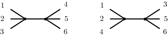
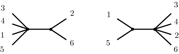
A cross-ratio is a rational number associated to four collinear points. It encodes the relative position of these four points to each other. It is invariant under projective transformations and can therefore be used as a constraint that four points on \(\mathbb {P}^1\) should satisfy. So a cross-ratio can be viewed as a condition on elements of the moduli space of n-pointed rational stable maps to a toric variety. Tropical cross-ratios were first introduced by Mikhalkin under the name “tropical double ratio” in [23] and can be thought of as paths of fixed lengths in a tropical curve. More precisely: A parameterized plane rational tropical curve (alternatively: tropical stable map) is a 1-dimensional polyhedral complex (mapped to \(\mathbb {R}^2\) satisfying the balancing condition) whose first Betti number is zero and whose unbounded polyhedra (points on a tropical curve are contracted unbounded polyhedra) are uniquely labeled (see Definition 2.16). A tropical cross-ratio consists of two pieces of information: First a pair of pairs of labels of unbounded polyhedra such that all occuring labels are pairwise different and second a length. A parameterized plane rational tropical curve satisfies a tropical cross-ratio if forgetting the map to \(\mathbb {R}^2\) and all unbounded polyhedra which are not given in the cross-ratio leaves an abstract tropical curve whose bounded parts’ lengths sum up to the given length in the cross-ratio such that forgetting the bounded parts splits the four remaining labels into the two given pairs—see Fig. 1 for an example and Definition 3.1 for more details. It is natural to ask: Given point conditions \(p_1,\dots ,p_n\) and cross-ratio constraints \(\lambda _1,\dots ,\lambda _l\) in such a way that there are only finitely many parametrized rational tropical curves of a given degree in a toric surface satisfying them, then
-
(1)
How many of these curves are there and what are their multiplicities?
-
(2)
Can we construct them?
These questions motivated the study in this paper. Recall that applying tropical geometry to an enumerative problem happens in two steps: use a correspondence theorem, then use combinatorics. The correspondence theorem we are going to use is provided by Tyomkin in [31]. It also describes the multiplicities with which parameterized rational tropical curves have to be counted when they satisfy cross-ratio constraints.
Our approach to answer questions (1) and (2) can be subdivided into two steps. The first step is to develop a notion of degenerated tropical cross-ratios that helps us to simplify the combinatorics. Notice that Tyomkin’s correspondence theorem provides the multiplicities only in the non-degenerated case. The tradeoff when simplifying the combinatorics by considering degenerated tropical cross-ratios is that the multiplicities coming from the cross-ratio constraints get more involved. The second step to answer questions (1) and (2) is to explicitly construct all parameterized rational tropical curves that satisfy the given point and degenerated cross-ratio conditions using combinatorial methods. We want to explain these two steps and the methods used more precisely:

Left: a degree two plane tropical curve that is fixed by two points \(q_1,q_2\) and three cross-ratios: the red length associated to the four labels (16|23), the blue length associated to the four labels \((1q_2|35)\) and the green length associated to the four labels (23|45) are fixed. Right: degenerating the cross-ratio associated to the green path means shrinking the green path, thus producing a 4-valent vertex (with two unbounded edges on top of each other) (color figure online)
1.1 Degenerated cross-ratios
In Sect. 3 a generalization of Mikhalkin’s definition of tropical cross-ratios is introduced that allows us to use tropical intersection theory in order to degenerate tropical cross-ratios. If we think of a cross-ratio as a path of fixed length in a tropical curve, then a degenerated cross-ratio is a path of length zero—see Fig. 1. Obviously, the set of tropical curves satisfying given conditions becomes easier when degenerating the cross-ratios. The difficult part is to determine the multiplicities with which we have to count such curves. These multiplicities have a local description, which we present in Theorem 3.20 together with the fact that the number of parameterized tropical curves (counted with multiplicity) satisfying point and cross-ratio conditions stays invariant when degenerating the cross-ratios. The techniques used to prove Theorem 3.20 are tropical moduli spaces and tropical intersection theory.
Moduli spaces of abstract rational tropical curves were studied in [23]. They also show up in the study of the tropical Grassmannian as the space of trees [6, 29]. It turns out that these tropical moduli spaces are tropicalizations of the corresponding moduli spaces in algebraic geometry in a suitable embedding [17, 30]. Tropicalizations of moduli spaces of curves of higher genus (in a toroidal and non-Archimedean setting) were studied by Abramovich, Caporaso and Payne [1]. The theory of rational tropical stable maps was introduced by Gathmann, Kerber and Markwig in [16]. Recently, Ranganathan [24] tropicalized the moduli space of stable rational maps to toric surfaces using logarithmic and non-Archimedean geometry. An excellent overview of the current development concerning compactifications of moduli spaces and tropical moduli spaces can be found in [12].
We use tropical intersection theory on moduli spaces of rational stable maps, building on Allermann and Rau [3, 26]. Katz [18] related tropical intersection theory to intersection theory on toric varieties studied by Fulton and Sturmfels in [14]. For matroidal fans (i.e. tropicalizations of linear spaces) Shaw offers in [27] a framework of tropical intersection theory. Tropical intersection theory is still an active area of research.
All in all degenerating cross-ratios is a natural approach in the following sense: A parameterized rational tropical curve satisfying non-degenerated conditions can be degenerated to a parameterized rational tropical curve that satisfies degenerated conditions itself. This observation allows us to answer question (2) if we can construct parameterized rational tropical curves that satisfy degenerated conditions. We offer an algorithm for this construction in Sect. 4.
1.2 Combinatorial methods
Both the lattice path algorithm and floor diagrams are well-known combinatorial tools in tropical geometry. In Sect. 4 we generalize the lattice path algorithm to a cross-ratio lattice path algorithm. Lattice paths were used in [21] and [22] to construct curves satisfying point conditions. Since we want to find tropical curves that satisfy point and degenerated cross-ratio conditions, we need to generalize this approach. There are other generalizations (in particular [20]) of lattice paths that inspired our definition of cross-ratio lattice paths. The lattice path algorithm can also be extended to determine invariants connected to counts of real curves as well, see [28].
In Sect. 5 we prove Theorem 5.3, which states that the lattice path algorithm yields the number of rational parameterized tropical curves satisfying point and tropical cross-ratio conditions counted with multiplicity. Thus Theorem 5.3 answers question (1). Moreover, the cross-ratio lattice path algorithm we provide allows us to construct all tropical curves of a given degree that satisfy the given point conditions and the degenerated tropical cross-ratio constraints.
In Sect. 6 we restrict to curves in Hirzebruch surfaces and impose a restriction to our cross-ratios such that we can use simpler combinatorial objects than the ones we deal with when applying the cross-ratio lattice path algorithm. These simpler combinatorial objects are called cross-ratio floor diagrams. They are a generalization of floor diagrams. Floor diagrams are graphs that arise from so-called floor decomposed tropical curves by forgetting some information. Floor diagrams were introduced by Mikhalkin and Brugallé in [10] (and [11]) to give a combinatorial description of Gromov–Witten invariants of Hirzebruch surfaces. Floor diagrams have also been used to establish polynomiality of the node polynomials [13] and to give an algorithm to compute these polynomials in special cases—see [7]. Moreover, floor diagrams have been generalized, for example in case of \(\Psi \)-conditions, see [8], or for counts of curves relative to a conic [9].
Theorem 6.14 states that counting floor diagrams with multiplicities yields the same numbers as counting parameterized rational tropical curves with multiplicities that satisfy point and tropical cross-ratio conditions. Hence floor diagrams offer (besides the cross-ratio lattice path algorithm) another (simpler) way of answering question (1).
2 Preliminaries
In this preliminary section we give a short introduction to tropical intersection theory and tropical moduli spaces as needed in this paper. We fix the following conventions: polytopes are convex, and we work over a non-Archimedean closed field of characteristic zero.
2.1 Tropical intersection theory
This subsection summarizes intersection theoretic background from [2,3,4].
Definition 2.1
(Normal vectors and balanced fans) Let \(V:=\Gamma \otimes _{\mathbb {Z}}\mathbb {R}\) be the real vector space associated to a given lattice \(\Gamma \) and let X be a fan in V. The lattice generated by \({\text {span}}(\kappa )\cap \Gamma \), where \(\kappa \) is a cone of X, is denoted by \(\Gamma _\kappa \). Let \(\sigma \) be a cone of X and \(\tau \) be a face of \(\sigma \) of dimension \(\dim (\tau )=\dim (\sigma )-1\) (we write \(\tau <\sigma \)). A vector \(u_{\sigma }\in \Gamma _\sigma \) that generates \(\Gamma _\sigma / \Gamma _\tau \) such that \(u_\sigma +\tau \subset \sigma \) defines a class \(u_{\sigma / \tau }:=[u_\sigma ]\in \Gamma _\sigma / \Gamma _\tau \) that does not depend on the choice of \(u_\sigma \). This class is called normal vector of \(\sigma \) relative to \(\tau \).
X is a weighted fan of dimension k if X is of pure dimension k and there are weights on its facets (i.e. its k-dimensional faces), that is there is a map \(\omega _X:X^{(k)}\rightarrow \mathbb {Z}\). The number \(\omega _X(\sigma )\) is called weight of the facet \(\sigma \) of X. To simplify notation, we write \(\omega (\sigma )\) if X is clear. Moreover, a weighted fan \((X,\omega _X)\) of dimension k is called a balanced fan of dimension k if
holds in \(V/\langle \tau \rangle _{\mathbb {R}}\) for all faces \(\tau \) of dimension \(\dim (\tau )=\dim (\sigma )-1\).
Definition 2.2
(Affine cycles) Let \(V:=\Gamma \otimes _{\mathbb {Z}}\mathbb {R}\) be the real vector space associated to a given lattice \(\Gamma \). A tropical fan X (of dimension k) is a balanced fan of dimension k in V and \([(X,\omega _X)]\) denotes the refinement class of X with weights \(\omega _X\) (see Definition 2.8 and Construction 2.10 of [3]). Such a class is also called an affine (tropical) k-cycle in V. Denote the set of all affine k-cycles in V by \(Z^{\text {aff}}_k(V)\). For a fan X in V, we may also define an affine k-cycle in X as an element \([(Y,\omega _Y)]\) of \(Z^{\text {aff}}_k(V)\) such that the support of Y with nonzero weights lies in the support of X (see Definition 2.15 of [3]). Define \(|[(X,\omega _X)]|:=X^*\), where \(X^*\) denotes the support of X with nonzero weights.
The set \(Z^{\text {aff}}_k(V)\) (resp. \(Z^{\text {aff}}_k([(X,\omega _X)])\)) can be turned into an abelian group by taking unions while refining appropriately.
Definition 2.3
(Rational functions) Let \([(X,\omega _X)]\) be an affine k-cycle. A (nonzero) rational function on \([(X,\omega _X)]\) is a continuous piecewise linear function \(\varphi :|[(X,\omega _X)]|\rightarrow \mathbb {R}\), i.e. there exists a representative \((X,\omega _X)\) of \([(X,\omega _X)]\) such that on each cone \(\sigma \in X\) the map \(\varphi \) is the restriction of an integer affine linear function. The set of (nonzero) rational functions of \([(X,\omega _X)]\) is denoted by \(\mathcal {K}^*([(X,\omega _X)])\).
Define \(\mathcal {K}\left( [(X,\omega _X)]\right) :=\mathcal {K}^*([(X,\omega _X)])\cup \{-\infty \}\) such that \((\mathcal {K}([(X,\omega _X)]),{\text {max}},+)\) is a semifield, where the constant function \(-\infty \) is the “zero” function.
Definition 2.4
(Divisor associated to a rational function) Let \([(X,\omega _X)]\) be an affine k-cycle in \(V=\Gamma \otimes _{\mathbb {Z}}\mathbb {R}\) and \(\varphi \in \mathcal {K}^*([(X,\omega _X)])\) a rational function on \([(X,\omega _X)]\). Let \((X,\omega )\) be a representative of \([(X,\omega _X)]\) on whose cones \(\varphi \) is affine linear and denote these linear pieces by \(\varphi _\sigma \). We denote by \(X^{(i)}\) the set of all i-dimensional cones of X. We define \({\text {div}}(\varphi ):=\varphi \cdot [(X,\omega _X)]:= [(\bigcup _{i=0}^{k-1}X^{(i)},\omega _{\varphi })]\in Z^{\text {aff}}_{k-1}([(X,\omega _X)])\), where
and the \(v_{\sigma /\tau }\) are arbitrary representatives of the normal vectors \(u_{\sigma /\tau }\). If \([(Y,\omega _Y)]\) is an affine k-cycle in \([(X,\omega _X)]\), we define \(\varphi \cdot [(Y,\omega _Y)]:=\varphi \mid _{|[(Y,\omega _Y)]|}\cdot [(Y,\omega _Y)]\).
Example 2.5
Let \([(X,\omega _X)]\) be the affine 1-cycle with representative \((X,\omega _X)\) whose weights are all 1 and whose 1-dimensional rays are given by \(-e_x,-e_y,e_x+e_y\), where \(e_x,e_y\) are the vectors of the standard basis of \(\mathbb {R}^2\) such that \(X\subset \mathbb {R}^2\). Then
is a rational function on \([(X,\omega _X)]\) and \((X,\omega _X)\) is a representative such that \(\varphi \) is integer linear affine on each cone. The divisor associated to \(\varphi \), namely \(\varphi \cdot X\), is given by the 1-skeleton of X which is just one point (namely \(0\in \mathbb {R}^2\)) and that point has weight 1. We calculate this weight as an example: Let \(\tau =0\in \mathbb {R}^2\), \(\sigma _1={\text {cone}}\left( -e_x \right) ,\sigma _2={\text {cone}}\left( -e_y\right) \) and \(\sigma _3={\text {cone}}\left( e_x+e_y\right) \) be cones of X. Applying Definition 2.4, we get
because \(\varphi _{\sigma _1},\varphi _{\sigma _2},\varphi _{\tau }\equiv 0\) and \(\varphi _{\sigma _3}\left( e_x+e_y \right) =\max (1,1,0)\).
Definition 2.6
(Affine intersection product) Let \([(X, w_X)]\) be an affine k-cycle. The subgroup of globally linear functions in \(\mathcal {K}^*([(X, w_X)])\) with respect to \(+\) is denoted by \(\mathcal {O}^*([(X, w_X)])\). We define the group of affine Cartier divisors of \([(X, w_X)]\) to be the quotient group \({\text {Div}}([(X, w_X)]):=\mathcal {K}^*([(X, w_X)])/\mathcal {O}^*([(X, w_X)])\). Let \([\varphi ]\in {\text {Div}}([(X, w_X)])\) be a Cartier divisor. The divisor associated to this function is denoted by \({\text {div}}([\varphi ]):={\text {div}}(\varphi )\) and is well-defined. The following bilinear map is called affine intersection product
Definition 2.7
(Morphisms of fans) Let X be a fan in \(V=\Gamma \otimes _{\mathbb {Z}}\mathbb {R}\) and Y a fan in \(V'=\Gamma '\otimes _{\mathbb {Z}}\mathbb {R}\). A morphism \(f:X\rightarrow Y\) is a \(\mathbb {Z}\)-linear map from \(|X|\subseteq V\) to \(|Y|\subseteq V'\) induced by a \(\mathbb {Z}\)-linear map on the lattices. A morphism of weighted fans is a morphism of fans. A morphism of affine cycles \(f:[(X,\omega _X)]\rightarrow [(Y,\omega _Y)]\) is a morphism of weighted fans \(f:X^*\rightarrow Y^*\) that is independent of the choice of representatives, where \(X^*\) (resp. \(Y^*\)) denotes the support of X (resp. Y) with nonzero weight.
Definition 2.8
(Push-forward of affine cycles) Let \(V=\Gamma \otimes _{\mathbb {Z}}\mathbb {R}\) and \(V'=\Gamma '\otimes _{\mathbb {Z}}\mathbb {R}\). Let \([(X, w_X)]\in Z^{\text {aff}}_m(V)\) and \([(Y, w_Y)]\in Z^{\text {aff}}_n(V')\) be cycles with representatives \((X,\omega _X)\) and \((Y,\omega _Y)\). Let \(f:X\rightarrow Y\) be a morphism. Choosing a refinement of \((X,\omega _X)\), the set of cones
is a tropical fan in \(V'\) of dimension m with weights
for all \(\sigma '\in f_*X^{(m)}\). The equivalence class of \((f_*X,\omega _{f_*X})\) is uniquely determined by the equivalence class of \((X,\omega _X)\). For \([(Z,\omega _Z)]\in Z^{\text {aff}}_k([(X,\omega _X)])\) we define
The map
is well-defined, \(\mathbb {Z}\)-linear and \(f_*[(Z, w_Z)]\) is called push-forward of \([(Z, w_Z)]\) along f.
Definition 2.9
(Pull-back of Cartier divisors) Let \([(X, w_X)]\in Z^{\text {aff}}_m(V)\) and \([(Y, w_Y)]\in Z^{\text {aff}}_n(V')\) be cycles in \(V=\Gamma \otimes _{\mathbb {Z}}\mathbb {R}\) and \(V'=\Gamma '\otimes _{\mathbb {Z}}\mathbb {R}\). Let \(f:[(X, w_X)]\rightarrow [(Y, w_Y)]\) be a morphism. The map
is well-defined, \(\mathbb {Z}\)-linear and \(f^*[h]\) is called pull-back of [h] along f.
So far, we introducted affine cycles only. Affine cycles are building blocks of abstract cycles. Since the whole “affine-to-abstract”-procedure is quite technical, we omit it here and refer to section 5 of [3] instead. For our purposes the following definition of abstract cycles is sufficient:
Definition 2.10
(Abstract cycles) An abstract k-cycle C is a class under a refinement relation of a balanced polyhedral complex of pure dimension k which is locally isomorphic to tropical fans.
Remark 2.11
(Rational functions on abstract cycles) In the same way rational functions on affine cycles led to an affine intersection product, one can also consider rational functions on abstract cycles to obtain a intersection product. Again, we want to omit technicalities and refer to Definition 6.1 of [3] instead. The main point of considering rational functions on abstract cycles is that they are no longer piecewiese linear but pieceweise affine linear.
As we see below, it happens that we start with an affine cycle \([(X,\omega _X)]\) and want to intersect it with a rational function f that is pieceweise affine linear. In order to do so, we need to refine \([(X,\omega _X)]\) in such a way that f is linear on faces. Hence \([(X,\omega _X)]\) becomes a polyhedral complex which is a representative of an abstract cycle C. Then we can intersect f with C.
In the following we want to restrict to tropical intersection theory on \(\mathbb {R}^n\).
Definition 2.12
(Degree map) Let \(A_0(\mathbb {R}^n)\) denote the set of abstract 0-cycles in \(\mathbb {R}^n\) up to rational equivalence. The map
is a well-defined morphism and for \(D\in A_0(\mathbb {R}^n)\) the number \({\text {deg}}(D)\) is called the degree of D.
Remark 2.13
(Rational equivalence) Concepts like pull-backs and push-forwards carry over to abstract cycles. Moreover, there is a concept of rational equivalence of abstract cycles (section 8 of [3]). When we consider abstract cycles, we usually consider them up to this equivalence relation. The most important facts about rational equivalence that we use are the following:
-
(a)
Pull-backs of rationally equivalent cycles are rationally equivalent.
-
(b)
If two 0-dimensional cycles are rationally equivalent, then their degrees are the same.
-
(c)
Two cycles in \(\mathbb {R}^n\) that only differ by a translation are rationally equivalent.
2.2 Tropical moduli spaces
This subsection collects background on tropical moduli spaces following [16].
Definition 2.14
(Moduli space of abstract tropical curves of genus zero) An abstract rational tropical curve is a metric tree \(\Gamma \) with unbounded edges called ends and with \({\text {val}}(v)\ge 3\) for all vertices \(v\in \Gamma \). It is called rational n-marked tropical curve of genus zero \((\Gamma ,x_1,\dots ,x_n)\) if \(\Gamma \) has exactly n ends that are labeled with pairwise different \(x_1,\dots ,x_n\in \mathbb {N}\). Two n-marked tropical curves of genus zero \((\Gamma ,x_1,\dots ,x_n)\) and \((\tilde{\Gamma },\tilde{x}_1,\dots ,\tilde{x}_n)\) are isomorphic if there is a homeomorphism \(\Gamma \rightarrow \tilde{\Gamma }\) mapping \(x_i\) to \(\tilde{x}_i\) for all i and each edge of \(\Gamma \) is mapped onto an edge of \(\tilde{\Gamma }\) by an affine linear map of slope \(\pm 1\). The set \(\mathcal {M}_{0,n}\) of all n-marked tropical curves of genus zero up to isomorphism is called moduli space of n-marked tropical curves of genus zero. Forgetting all lengths of an n-marked tropical curve gives us its combinatorial type.
Remark 2.15
(\(\mathcal {M}_{0,n}\) is a tropical fan) We have the distance map
and define \(v_I\) (\(I\subset \{1,\dots ,n\}, |I|\ge 2, |I^C|\ge 2\)) to be the image under dist of the n-marked tropical curve that has only one bounded edge of length one with markings I on one and markings \(I^C\) on the other side. Moreover, the map
induces (by abuse of notation) an injective map
If we choose
to be the lattice of \(\mathbb {R}^{n\atopwithdelims ()2}/{\text {Im}}(\phi )\), then \(\mathcal {M}_{0,n}\subseteq \mathbb {R}^{n\atopwithdelims ()2}/{\text {Im}}(\phi )\) is a tropical fan of pure dimension \(n-3\) with its fan structure given by combinatorial types, and with all weights equal one, i.e. \(\mathcal {M}_{0,n}\) represents an affine cycle in some \(\mathbb {R}^t\), see Fig. 2. This allows us to use tropical intersection theory on \(\mathcal {M}_{0,n}\).

One way of embedding the moduli space \(\mathcal {M}_{0,4}\) into \(\mathbb {R}^2\) centered at the origin of \(\mathbb {R}^2\). The length of a bounded edge of a tropical curve depicted above is given by the distance between the point in \(\mathcal {M}_{0,4}\) corresponding to this curve and the origin of \(\mathbb {R}^2\)
Definition 2.16
(Degree) Let \(\#\Delta \in \mathbb {N}_{>0}\). A set \(\Delta :=\lbrace (v_i,x_i)\rbrace _{i=1,\dots ,\#\Delta }\) of tuples is called degree if
-
(1)
\(0\ne v_i\in \mathbb {R}^2\) for all \(i=1,\dots ,\#\Delta \), and \(\langle v_1,\dots ,v_{\#\Delta }\rangle =\mathbb {R}^2\), and \(\sum _i v_i=0\).
-
(2)
\(x_i\in \mathbb {N}_{>0}\) for all \(i=1,\dots ,\#\Delta \), and \(x_i\ne x_j\) for all \(i\ne j\). An \(x_i\) is called label.
Let \(\Sigma \) be a 2-dimensional lattice polytope in \(\mathbb {R}^2\) with facets \(E_1,\dots ,E_m\) whose lattice lengths are denoted by \(|E_1|,\dots ,|E_m|\) and let \(e_1,\dots ,e_m\) be unordered partitions of \(E_1,\dots ,E_m\), that is \(e_i\) is a partition of \(E_i\) of some length denoted by \(l(e_i)\) for \(i=1,\dots ,m\). If
where \({\text {pnv}}(E_i)\) is the primitive normal vector of \(E_i^\perp \) for \(i=1,\dots ,m\), then \(\Delta \) is said to be associated to a polytope \(\Sigma \) with partitions \(e_1,\dots ,e_m\) and is referred to as \(\Delta \left( \Sigma (e_1,\dots ,e_m)\right) \).
Important special cases that we use later are the following:
-
If each entry of each partition \(e_i\) is one, then the associated degree is denoted by \(\Delta (\Sigma )\).
-
In case of degree d curves in \(\mathbb {P}^2\), the degree \(\Delta \) is defined as follows: Let \(\Sigma _d\) be the convex hull of \(\lbrace (0,0),(d,0),(d,0)\rbrace \in \mathbb {R}^2\) for some \(d\in \mathbb {N}_{>0}\), then \(\Delta _d\) is the degree associated to \(\Sigma _d\), where the labels are given by: vectors parallel to (and with the same direction as) \((-1,0)\in \mathbb {R}^2\) have labels \(1,\dots ,d\), vectors parallel to (and with the same direction as) \((0,-1)\) have labels \(d+1,\dots ,2d\) and vectors parallel to (and with the same direction as) (1, 1) have labels \(2d+1,\dots ,3d\).
-
In case of degree \((|\alpha |,|\beta |)\) curves of contact orders \(\alpha ,\beta \) in the first Hirzebruch surface, the degree \(\Delta \) is defined as follows: Let \(s\in \mathbb {N}_{>0}\) and \(b\in \mathbb {N}\). Let \(\alpha =(\alpha _1,\dots )\) be an unordered partition of \(b+s\), let \(\beta =(\beta _1,\dots )\) be an unordered partition of b and let \(\Sigma (\alpha ,\beta )\) be the convex hull of \(\lbrace (0,0),(s,0),(s,b),(0,b+s)\rbrace \in \mathbb {R}^2\). We associate the degree \(\Delta \left( \alpha ,\beta \right) \) to the polytope \(\Sigma (\alpha ,\beta )\), where the partition of the left facet is given by \(\alpha \) and the partition of the right facet is given by \(\beta \). Moreover, vectors parallel to (and with the same direction as) \((-1,0)\in \mathbb {R}^2\) have labels \(1,\dots , l(\alpha )\), vectors parallel to (and with the same direction as) (1, 0) have labels \(l(\alpha )+1,\dots ,l(\alpha )+l(\beta )\).
Definition 2.17
(Moduli space of rational tropical stable maps to \(\mathbb {R}^2\)) An n-pointed rational tropical stable map of degree \(\Delta \) to \(\mathbb {R}^2\) (alternatively: rational tropical curve with n points) is a tuple \((\Gamma ,x_1,\dots ,x_N,h)\), where \((\Gamma ,x_1,\dots ,x_N)\) is an N-marked rational tropical curve (with \(N=\#\Delta +n\) and \(x_{n+1},\dots ,x_{N}\) the labels given by \(\Delta \)) and \(h:\Gamma \rightarrow \mathbb {R}^2\) such that:
-
(a)
Let \(e\in \Gamma \) be an edge with length \(l(e)\in [0,\infty ]\), identify e with [0, l(e)] and denote the vertex of e that is identified with \(0\in [0,l(e)]=e\) by V. The map h is integer affine linear when restricted to e, i.e. \(h\mid _e:t\mapsto tv+a\) with \(a\in \mathbb {R}^2\) and \(v(e,V):=v\in \mathbb {Z}^2\), where v(e, V) is called direction vector of e at V and the weight of an edge (denoted by \(\omega (e)\)) is the \(\gcd \) of the entries of v(e, V). If \(e=x_i\in \Gamma \) is an end, then \(v(x_i)\) denotes the direction vector of \(x_i\) pointing away from its one vertex it is adjacent to.
-
(b)
If \(i>n\), then the direction vector \(v(x_i)\) of an end labeled with \(x_i\) is given by
$$\begin{aligned} v(x_i):=v_{i-n}, \end{aligned}$$where \(v_{i-n}\) is defined by \(\Delta \). If \(i\le n\), then the direction vector of the end labeled with \(x_i\) is zero. Ends with direction vector zero are called contracted ends or points.
-
(c)
The balancing condition
$$\begin{aligned} \sum _{\begin{array}{c} e\in \Gamma \text { an edge}, \\ V \text { vertex of }e \end{array}}v(e,V)=0 \end{aligned}$$holds for every vertex \(V\in \Gamma \).
Two n-pointed rational tropical stable maps of degree \(\Delta \), namely \((\Gamma ,x_1,\dots ,x_N,h)\) and \((\Gamma ' ,x_1', \dots , x_N',h')\), are isomorphic if there is an isomorphism \(\varphi \) of their underlying N-marked tropical curves of genus zero such that \(h'\circ \varphi =h\).
The set \(\mathcal {M}_{0,n}(\mathbb {R}^2,\Delta )\) of all n-pointed rational tropical stable maps of degree \(\Delta \) up to isomorphism is called moduli space of n-pointed rational tropical stable maps of degree \(\Delta \).
Remark 2.18
(\(\mathcal {M}_{0,n}(\mathbb {R}^2,\Delta )\) is a fan) The map
with \(N=\#\Delta +n\) is bijective and \(\mathcal {M}_{0,n}\left( \mathbb {R}^2,\Delta \right) \) is a tropical fan of dimension \(\#\Delta -1\), see Proposition 4.7 of [16]. Hence \(\mathcal {M}_{0,n}\left( \mathbb {R}^2,\Delta \right) \) represents an affine cycle in some \(\mathbb {R}^t\). This allows us to use tropical intersection theory on \(\mathcal {M}_{0,n}\left( \mathbb {R}^2,\Delta \right) \).
Definition 2.19
(Evaluation maps) For \(i=1,\dots ,n\), the map
is called i-th evaluation map. Under the identification from Remark 2.18 the i-th evaluation map is a morphism of fans \({\text {ev}}_i:\mathcal {M}_{0,N}\times \mathbb {R}^2 \rightarrow \mathbb {R}^2\), see Proposition 4.8 of [16]. This allows us to pull-back cycles via the evaluation map.
Example 2.20
(Pull-back of a point) A point \(p=(p_1,p_2)\in \mathbb {R}^2\) is an intersection product of two rational functions, e.g.
where x, y are the coordinates in \(\mathbb {R}^2\). The pull-back of the point p under \({\text {ev}}_i\) is defined to be
Definition 2.21
For \(n\ge 4\) the map
where \(\Gamma '\) is the stabilization (straighten 2-valent vertices) of \(\Gamma \) after removing its end marked by \(x_n\) is called the n-th forgetful map. Applied recursively, it can be used to forget several ends with markings in \(I^C\subset \{x_1,\ldots ,x_n\}\), denoted by \({\text {ft}}_I\), where \(I^C\) is the complement of \(I\subset \{x_1,\ldots ,x_n\}\). With the identification from Remark 2.18, and additionally forgetting the map to the plane, we can also consider
Any forgetful map is a morphism of fans. This allows us to pull-back cycles via the forgetful map.
2.3 Correspondence theorem
The tropical counterpart to calssical cross-ratios was first introduced by Mikhalkin under the name tropical double ratio in [23]. The correspondence theorem of [31] we use states that the number of classical curves satisfying point and cross-ratio conditions and the number of tropical curves satisfying point and tropical double ratio conditions are equal. Since different classical curves may tropicalize to the same tropical curve, each tropical curve has to be counted with a multiplicity. We recall the definition of these multiplicities. For that we stick to the notation used in [31], for more details see (4.1) of [31].
Definition 2.22
(Tropical double ratios defined by [23, 31]) Let \((\Gamma ,x_1,\dots ,x_N,h)\in \mathcal {M}_{0,n}\left( \mathbb {R}^2,\Delta \right) \). Let \(\lbrace \beta _{i_1},\beta _{i_3}\rbrace \) and \(\lbrace \beta _{i_2},\beta _{i_4}\rbrace \) be two sets of labels of ends of \(\Gamma \) such that \(\beta _{i_1},\dots ,\beta _{i_4}\) are pairwise different. A bounded edge \(\gamma \) of \(\Gamma \) separates \(\beta _{i_1},\beta _{i_2}\) from \(\beta _{i_3},\beta _{i_4}\) if \(\beta _{i_1},\beta _{i_2}\) belong to one of the two connected components of \(\Gamma \backslash \lbrace \gamma \rbrace \) and \(\beta _{i_3},\beta _{i_4}\) to another.
The tropical double ratio \(\lambda '_i\) of \(\lbrace \beta _{i_1},\beta _{i_2}\rbrace \) and \(\lbrace \beta _{i_3},\beta _{i_4}\rbrace \) is given by
where the sum goes over all bounded edges of \(\Gamma \) and \(|\gamma |\) is the length of a bounded edge and
See Fig. 3 for an example. Notice that by abuse of notation we do not incorporate the \(\beta _i\)’s into the notation of a tropical double ratio \(\lambda _i'\).

Schematic picture of the three cases of \(\epsilon (\gamma ,i)\) for \(\lambda _i'\) as in Definition 2.22 for a 4-marked curve. From left to right: \(\epsilon (\gamma ,i)=1,-1,0\)
Remark 2.23
(Tropical double ratios and tropicalizations) Note that tropical double ratios are indeed tropicalizations of classical cross-ratios (see Lemma 3.1 of [31]), i.e. given a classical curve that satisfies a classical cross-ratio, then its tropicalization satisfies a tropical double ratio which is given by applying the valuation map to the classical cross-ratio.
Definition 2.24
(Multiplicities) Let \(C=(\Gamma ,x_1,\dots ,x_N,h)\) be a tropical curve that satisfies given point conditions \(p_1,\dots ,p_n\) and tropical double ratios \(\lambda '_1,\dots ,\lambda '_l\).
Let \(x_1\) be the end of \(\Gamma \) that is contracted to \(p_1\) under h. We refer to the vertex adjacent to \(x_1\) in \(\Gamma \) as root vertex and orient all edges of \(\Gamma \) away from the root vertex. The head of a bounded edge \(\gamma \) is denoted by \(\mathfrak {h}(\gamma )\) and its tail by \(\mathfrak {t}(\gamma )\). Let \(V(\Gamma )\) be the set of vertices of \(\Gamma \) and let \(E^b(\Gamma )\) be the set of bounded edges of \(\Gamma \). We refer to a vertex of \(\Gamma \) as v and to a bounded edge of \(\Gamma \) as \(\gamma \) for now. The vertices adjacent to ends \(x_1,\dots ,x_N\) are denoted by \(v_1,\dots ,v_N\) and do not need to be different. Define the complex
given by the maps (that are defined copywise)
where \(a_v\) is the coordinate vector of h(v) and where (see Definition 2.17 for the notation of \(v(\gamma ,\mathfrak {t}(\gamma ))\))
and
Let \(\theta _\mathbb {Z}\) be the map from above in the complex (1)\(\otimes _\mathbb {Z}\mathbb {Z}\). Finally, we can define the multiplicity of C
which is equal to \(|\det (B)|\).
Theorem 2.25
(Correspondence Theorem 5.1 of [31]) Let \(\Sigma \) be a 2-dimensional lattice polytope and let \(X_\Sigma \) be its toric variety. Let \(q_1,\dots ,q_n\) be points in \(X_\Sigma \) and let \(\mu _1,\dots ,\mu _l\) be classical cross-ratio constraints. Let these conditions be in general position such that there is only a finite number of rational curves in \(X_\Sigma \) that fulfill them. Denote this number by \(N^{\text {class}}_{0,n}\left( \mu _1,\dots ,\mu _l \right) \). Let \(p_1,\dots ,p_n,\lambda '_1,\dots ,\lambda '_l\) be the tropicalizations (see Remark 2.23) of the conditions above. Then
holds, where \(N_{0,n}(\lambda '_1,\dots ,\lambda '_l)\) is the number of rational tropical curves of degree \(\Delta (\Sigma )\) that satisfy the point conditions \(p_1,\dots ,p_n\) and the tropical double ratio constraints \(\lambda '_1,\dots ,\lambda '_l\).
Example 2.26
When going through the (tropical) proof of Kontsevich’s formula [15], we can see that it allows us to determine the number of unlabeled tropical curves of degree \(\Delta _d\) satisfying point conditions and exactly one tropical double ratio constraint which involves two point conditions and two line conditions. In this case unlabeled means that non-contracted edges not involved in any tropical double ratio condition are not equipped with a label.
In case of \(d=3\), Kontsevich’s formula yields 40 unlabeled curves (counted with multiplicity). Moreover, the proof of Kontsevich’s formula allows us to actually draw these tropical curves. Hence we can determine the number of labeled curves by putting labels on ends, which yields 1440 labeled curves.
3 Tropical cross-ratios
In this section we introduce tropical cross-ratios and their degenerations from an intersection theoretic point of view. Given a tropical curve that satisfies degenerated cross-ratios, we express its multiplicity locally.
Definition 3.1
(Cross-ratios) A (tropical) cross-ratio \(\lambda '\) is an unordered pair of pairs of unordered numbers \((\beta _1\beta _2|\beta _3\beta _4)\) together with an element in \(\mathbb {R}_{>0}\) denoted by \(|\lambda '|\), where \(\beta _1,\dots ,\beta _4\) are pairwise distinct ends of a tropical curve of \(\mathcal {M}_{0,n}(\mathbb {R}^2,\Delta )\). We say that \(C\in \mathcal {M}_{0,n}(\mathbb {R}^2,\Delta )\) satisfies the cross-ratio constraint \(\lambda '\) if \(C\in {\text {ft}}^*_{\lambda '}(|\lambda '| )\cdot \mathcal {M}_{0,n}(\mathbb {R}^2,\Delta )\), where \(|\lambda '|\) is the canonical local coordinate of the ray \((\beta _1\beta _2|\beta _3\beta _4)\) in \(\mathcal {M}_{0,4}\).
Remark 3.2
Definition 3.1 generalizes Definition 2.22 of tropical double ratios used by Mikhalkin and Tyomkin since we can find a suitable projektion \(\pi :\mathcal {M}_{0,4}\rightarrow \mathbb {R}\) shrinking on ray to zero, sending another one to \(\mathbb {R}_{>0}\) and the last one to \(\mathbb {R}_{<0}\) such that \(\pi \circ {\text {ft}}_{\lambda '}\) coincides with Definition 2.22. In particular, Theorem 2.25 holds for our notion of tropical cross-ratios.
Definition 3.3
(General position I) Let \(p_1,\dots ,p_n\) be points in \(\mathbb {R}^2\) and \(\lambda '_1,\dots ,\lambda '_l\) be cross-ratios that have pairwise distinct pairs of unordered numbers. These conditions are in general position if \(\prod _{j=1}^{l}{\text {ft}}_{\lambda '_j}^*\left( |\lambda '_j|\right) \cdot \prod _{i=1}^n{\text {ev}}_i^*( p_i)\cdot \mathcal {M}_{0,n}(\mathbb {R}^2,\Delta )\) is a nonempty finite set that is contained in the union of the interiors of top-dimensional polyhedra of \(\mathcal {M}_{0,n}(\mathbb {R}^2,\Delta )\) and \(n+l=\#\Delta -1\). We say that \(p_1,\dots ,p_{n'},\lambda _1,\dots ,\lambda _{l'}\) with \(n'+l'<\#\Delta -1\) are in general position if there are \(p_{n'+1},\dots ,p_n,\lambda '_{l'+1},\dots ,\lambda '_l\) such that \(n+l=\#\Delta -1\) and \(p_1,\dots ,p_n,\lambda '_1,\dots ,\lambda '_l\) are in general position. If \(p_1,\dots ,p_n,\lambda '_1,\dots ,\lambda '_l\) with \(n+l=\#\Delta -1\) are in general position, we define
the number of rational tropical curves of degree \(\Delta \) satisfying the point conditions \(p_i\) and the cross-ratio conditions \(\lambda '_i\). Denote by \(\mathcal {C}_{0,n}( \lambda '_1,\dots ,\lambda '_l)\) the set of tropical curves contributing to \(N_{0,n}(\lambda '_1,\dots ,\lambda '_l)\).
Remark 3.4
The numbers \(N_{0,n}(\lambda '_1,\dots ,\lambda '_l)\) are independent of the exact positions of the points since two sets of n points are rationally equivalent and so their pull-backs are rationally equivalent leading to the same degree (see Remark 2.13). Notice also that all points in \(\mathcal {M}_{0,4}\) are rationally equivalent using Remark 2.13 since \(\mathcal {M}_{0,4}\) can be embedded (cf. Fig. 2) by a morphism into \(\mathbb {R}^2\) and all points of \(\mathbb {R}^2\) are rationally equivalent. Hence the numbers \(N_{0,n}(\lambda '_1,\dots ,\lambda '_l)\) are independent of the lengths \(|\lambda '_i|\) of the cross-ratios. In particular, the lengths can be zero. This observation is crucial and is used extensively later. Moreover, \(N_{0,n}(\lambda '_1,\dots ,\lambda '_l)\) does not depend on the partition of the four entries of each cross-ratio into pairs.
Note that the intersection theoretic definition of tropical cross-ratios automatically assigns a multiplicity to each tropical curve satisfying given point conditions and cross-ratio constraints. In our case, Lemma 1.2.9 of [25] states that the intersection theoretic multiplicity of a tropical curve C is the absolute value of the determinant of the so called \({\text {ev}}\)-\({\text {ft}}\)-matrix which is given by the locally (around C) linear maps \({\text {ev}}:\mathcal {M}_{0,n}(\mathbb {R}^2,\Delta )\rightarrow \mathbb {R}^{2n}\) and \({\text {ft}}:\mathcal {M}_{0,n}(\mathbb {R}^2,\Delta )\rightarrow \mathcal {M}_{0,4}\), where the coordinates on \(\mathcal {M}_{0,n}(\mathbb {R}^2,\Delta )\) and \(\mathcal {M}_{0,4}\) are the bounded edges’ lengths.
Often, tropical intersection theory yields multiplicities needed for correspondence theorems, which enables us to count tropical curves by means of tropical intersection theory on tropical moduli spaces. The same holds true for the counts of curves satisfying cross-ratio conditions we consider here. We prove this in the following proposition, using methods well-known to the experts in the area.
Proposition 3.5
Let C be a tropical curve contributing to (2). The intersection theoretic multiplicity of C coincides with \(m_\mathbb {C}(\Gamma ,h)\) defined in Definition 2.24.
Proof
Let \(C=(\Gamma ,x_1,\dots ,x_N,h)\) be a tropical curve that contributes to \(N_{0,n}(\lambda '_1,\dots ,\lambda '_l)\). In terms of tropical intersection theory the multiplicity of C is given by \(|\det (A)|\), where A is the \({\text {ev}}\)-\({\text {ft}}\)-matrix that is given by the (around C) linear maps \({\text {ev}},{\text {ft}}\) and the lengths of the edges as coordinates on the moduli space. We want to sketch how to prove that \(|\det (A)|\) and \(|\det (B)|\) (from Definition 2.24) are equal. For that, we start with the following complex
where the first summand on the left belongs to the root vertex defined in Definition 2.24. There are maps between the complex above and the complex (1) in the following way: Let \(\alpha _2:N_2\rightarrow M_2\) be the canonical embedding and let
be a map where a is the coordinate of the root vertex, \(e_i\) is the length of the edge \(\gamma _i\) and \(u_{e_i}\) is the primitive direction vector of \(\gamma _i\). Moreover, we choose \(a+\sum \pm e_i u_{e_i}\) in such a way that it is the shortest path between the root vertex and the vertex associated to the j-th contracted end depending on which entry of the vector in the image we are considering (the choice of ± should be consistent with the orientation on \(\Gamma \)). Note that \(\alpha _1,\alpha _2\) are both injective and that the diagram given by the maps \(A,B,\alpha _1,\alpha _2\) commutes. This commutative diagram extends to the commutative diagram shown below. By definition
Considering the definitions of \(B,\zeta _2\), we can see that \(\zeta _2\circ B\) is surjective. Hence C is surjective. Since C is a surjective morphism of free module of the same rank it is an isomorphism. Therefore \({\text {coker}}\alpha _3\) vanishes which guarantees that \(\alpha _3\) is surjective. The map \(\partial \) which we obtain from applying the snake lemma yields that G vanishes. Therefore \(\alpha _3\) is an isomorphism. Thus
follows.

\(\square \)
The strength of our intersection theoretic definition of tropical cross-ratios is that it allows us to degenerate tropical cross-ratios easily. For that note that from an intersection theoretic point of view it does not matter if we pull-back \(0\in \mathcal {M}_{0,4}\) instead of a nonzero point.
Definition 3.6
(Cross-ratios with \(|\lambda |=0\)) A (tropical) cross-ratio \(\lambda \) with \(|\lambda |=0\) (or degenerated cross-ratio) is defined as a set \(\lbrace \beta _1,\dots ,\beta _4\rbrace \), where \(\beta _1,\dots ,\beta _4\) are pairwise distinct ends of a tropical curve \(\mathcal {M}_{0,n}(\mathbb {R}^2,\Delta )\). We say that \(C\in \mathcal {M}_{0,n}(\mathbb {R}^2,\Delta )\) satisfies the cross-ratio constraint \(\lambda \) (with \(|\lambda |=0\)) if \(C\in {\text {ft}}^*_\lambda (0 )\cdot \mathcal {M}_{0,n}(\mathbb {R}^2,\Delta )\). Notice that \(|\lambda |\) does not denote the number of elements in the set \(\lambda \) here. We use the symbol \(\#\) to indicate that we mean the number of elements in a set.
Another way to think about a cross-ratio \(\lambda \) with \(|\lambda |=0\) is that \(\lambda \) is the degeneration of cross-ratios \(\lambda '_j, j\in \mathbb {N}\) which have the same pairs of unordered numbers and \(|\lambda '_j|\rightarrow 0\) for \(j\rightarrow \infty \), where the pairs become a set in the limit. Because of Remark 3.4 it makes sense to refer to \(\lambda \) as the degeneration of \(\lambda '_j\) for some \(j\in \mathbb {N}\).
Definition 3.7
(General position II) Let \(\lambda _1,\dots ,\lambda _{l'}\) be cross-ratios with \(|\lambda _j|=0\) for \(j=1,\dots ,l'\). These cross-ratios are in general position if there are general positioned cross-ratios \(\lambda '_1,\dots ,\lambda '_{l'}\) such that \(\lambda _j\) is the degeneration of \(\lambda '_j\) for \(j=1,\dots ,l'\). More precisely, points \(p_1,\dots ,p_n\) in \(\mathbb {R}^2\), cross-ratios \(\lambda _1,\dots ,\lambda _{l'},\lambda _{l'+1},\dots ,\lambda _l\) with \(|\lambda _j|=0\) for \(j=1,\dots ,l'\) and \(|\lambda _j|>0\) otherwise are in general position if \(p_1,\dots ,p_n,\lambda '_1,\dots ,\lambda '_{l'},\lambda _{l'+1},\dots ,\lambda _l\) are in general position, where \(\lambda _j\) is the degeneration of \(\lambda '_j\) for \(j=1,\dots ,l'\).
Notation 3.8
We want to fix the following conventions. If we mention a set of conditions, then we assume that these conditions are in general position and that the cross-ratio constraints are totally ordered by their lengths, i.e. \(|\lambda _1|>|\lambda _2|>\dots \). Point conditions are always denoted by \(p_1,\dots ,p_n\). Cross-ratios are denoted by \(\lambda _i'\), where we have \(l'\) of these cross-ratios if the intersection defined by the conditions \(p_1,\dots ,p_n,\lambda _1',\dots ,\lambda _{l'}'\) is not a 0-dimensional cycle, and we have l cross-ratios if the intersection defined by the conditions \(p_1,\dots ,p_n,\lambda _1',\dots ,\lambda _{l}'\) is 0-dimensional. If we write \(\lambda _i\), then \(\lambda _i\) is the degeneration of \(\lambda _i'\). It may also happen that we need classical (i.e. non-tropical) cross-ratios. A classical cross-ratio is denoted by \(\mu _i\) and its tropical counterpart obtained from applying the valuation map of the ground field is denoted by \(\lambda _i'\).
Our next aim is to describe the multiplicity of a curve that satisfies point conditions and degenerated cross-ratio conditions. For that we observe that degenerating a cross-ratio means to shrink an edge, i.e. degenerating the tropical curve satisfying it as well. Therefore the multiplicity of such a degenerated tropical curve C can be described in terms of the number of tropical curves degenerating to C.
Definition 3.9
(Resolving vertices w.r.t. a cross-ratio with \(|\lambda |=0\)) The combinatorial type of a polyhedron \(\tau \subset \mathcal {M}_{0,n}(\mathbb {R}^2,\Delta )\) (resp. \(\mathcal {M}_{0,m}\)) is denoted by \(\mathfrak {c}(\tau )\). Let \(\lambda _1,\dots ,\lambda _{l'}\) be degenerated cross-ratios and let \(\tau \subset \mathcal {M}_{0,n}(\mathbb {R}^2,\Delta )\) be some polyhedron. The set \(\lambda _v\) of cross-ratios associated to a vertex v of \(\mathfrak {c}(\tau )\) consists of the cross-ratios \(\lambda _j\) such that the image of v under \({\text {ft}}_{\lambda _j}\) is 4-valent. If
holds, then we say that v is resolved according to \(\lambda '_i\) (we use Notation 3.8) if we replace v by two vertices \(v_1,v_2\) that are connected by a new edge such that
is a union of pairwise disjoint sets and
holds for \(k=1,2\).
Example 3.10
In this example we want to point out that resolving a vertex according to a cross-ratio is not unique. It is neither unique in the sense (A) that the edges adjacent to \(v_1,v_2\) are uniquely determined nor in the (weaker) sense (B) that the \(\lambda _{v_i}\) are uniquely determined.
Let \(\tau \) be the 0-dimensional cell of \(\mathcal {M}_{0,6}\), that is \(\mathfrak {c}(\tau )\) has only one vertex v to which all ends are adjacent to. We choose the following cross-ratios:
-
(A)
If we resolve v according to \(\lambda '_3\), we have at least two choices shown in the figure below.
-
(B)
If we choose another \(\lambda '_3\), namely \(\lambda '_3=(15|26)\), we also have at least two choices shown in the figure below.


Lemma 3.11
For notation, see Notation 3.8. The intersection product \(X:=\prod _{j=1}^{l'}{\text {ft}}_{\lambda _j}^*( 0)\cdot \mathcal {M}_{0,n}(\mathbb {R}^2,\Delta )\) lies in \(\mathcal {M}_{0,n}(\mathbb {R}^2,\Delta )^{(l')}\) and its top-dimensional polyhedra are top-dimensional polyhedra \(\tau \) of \(\mathcal {M}_{0,n}(\mathbb {R}^2,\Delta )^{(l')}\) such that for all vertices v of \(\mathfrak {c}(\tau )\)
holds and the weight of a top-dimensional polyhedron \(\tau \) of X is given recursively by
where the sum runs over all top-dimensional polyhedra of \(\prod _{j=2}^{l'}{\text {ft}}_{\lambda _j}^*( 0)\cdot \mathcal {M}_{0,n}(\mathbb {R}^2,\Delta )\) such that \(\mathfrak {c}(\sigma )\) is given by resolving the vertex \(v\in \mathfrak {c}(\tau )\), that is defined by \(\lambda _1\in \lambda _v\), according to \(\lambda '_1\). In particular, all weights of X are non-negative.
Note that the intersection product X above does not depend on the non-degenerated cross-ratios \(\lambda '_1,\dots ,\lambda '_{l'}\) that degenerate to \(\lambda _1,\dots ,\lambda _l\). We consider X up to rational equivalence. We use \(\lambda '_1,\dots ,\lambda '_{l'}\) to describe a representative of X under this equivalence relation.
Proof
Let \(\lambda '_1,\dots ,\lambda '_{l'}\) be cross-ratios such that \(\lambda _j\) is the degeneration of \(\lambda '_j\) for \(j=1,\dots ,l'\). The pull-back of 0 along \({\text {ft}}_{\lambda _j}\) is given by a Cartier divisior \(\max ({\text {ft}}_{\lambda _j}(\star ),0)\) (see Example 2.5), where \(\max (\star ,\star ,0):(x,y)\mapsto \max (x,y,0)\) is a Cartier divisor on \(\mathcal {M}_{0,4}\subset \mathbb {R}^2\) (see Fig. 2). Note that \(\max ({\text {ft}}_{\lambda _j}(\star ),0)\) is a linear function on every cell of \(\mathcal {M}_{0,n}(\mathbb {R}^2,\Delta )\) for \(j=1,\dots ,l'\). Therefore no refinement of \(\prod _{j\ne i}{\text {ft}}_{\lambda _j}^*( 0)\cdot \mathcal {M}_{0,n}(\mathbb {R}^2,\Delta )\) is necessary when intersecting with some \({\text {ft}}_{\lambda _i}^*( 0)\). Hence X lies in the codimension-\(l'\)-skeleton of \(\mathcal {M}_{0,n}(\mathbb {R}^2,\Delta )\). Moreover, every intersection with a Cartier divisor lowers the dimension by one, so the dimension of X is exactly the dimension of top-dimensional cells of the codimension-\(l'\)-skeleton of \(\mathcal {M}_{0,n}\left( \mathbb {R}^2,\Delta \right) \).
To prove the last part of the lemma, we set \(m=n+\#\Delta \) and identify
as in Remark 2.18 such that it is sufficient to prove the statements for \(\mathcal {M}_{0,m}\) because cross-ratio constraints only fix a tropical curve up to translation in \(\mathbb {R}^2\). To do so, we use induction on the number of cross-ratio constraints. Let \(m\in \mathbb {N}_{>3}\).
We start with one cross-ratio \(\lambda _1=\lbrace \beta _1,\dots ,\beta _4\rbrace \) with \(|\lambda _1|=0\). Obviously, a top-dimensional polyhedron \(\tau \) of \({\text {ft}}^*_{\lambda _1}\left( 0 \right) \cdot \mathcal {M}_{0,m}\) is a top-dimensional polyhedron \(\mathcal {M}_{0,m}^{(1)}\) such that \({\text {val}}(v)=3+\#\lambda _v\) holds for the only 4-valent vertex v of \(\mathfrak {c}(\tau )\) since \(\#\lambda _v=\#\lbrace \lambda _1\rbrace =1\). Note that the three resolutions of v correspond to three top-dimensional polyhedra \(\sigma _{(\beta _1\beta _2|\beta _3\beta _4)},\sigma _{(\beta _1\beta _3|\beta _2\beta _4)},\sigma _{(\beta _1\beta _4|\beta _2\beta _3)}\) of \(\mathcal {M}_{0,m}\) that arise from inserting a new edge e, where \(\sigma _{(\beta _1\beta _2|\beta _3\beta _4)}\) denotes the polyhedron where e separates \(\lbrace \beta _1,\beta _2 \rbrace \) from \(\lbrace \beta _3,\beta _4 \rbrace \). On two of the polyhedra \(\sigma _{(\beta _1\beta _2|\beta _3\beta _4)},\sigma _{(\beta _1\beta _3|\beta _2\beta _4)},\sigma _{(\beta _1\beta _4|\beta _2\beta _3)}\) the map \(\max \left( {\text {ft}}_{\lambda _j}(\star ),0\right) \) is the zero function and on one of that polyhedra it maps each point to the length of the edge that was obtained from resolving the vertex v. Which of the \(\sigma _{(\beta _1\beta _2|\beta _3\beta _4)},\sigma _{(\beta _1\beta _3|\beta _2\beta _4)}\) or \(\sigma _{(\beta _1\beta _4|\beta _2\beta _3)}\) are mapped to zero depends on the choice of coordinates of \(\mathcal {M}_{0,4}\subset \mathbb {R}^2\). Let \(v_{(\beta _1\beta _2|\beta _3\beta _4)}\) denote the direction vector in \(\mathcal {M}_{0,m}\) associated to a tropical curve that has only one edge of length one that separates the ends \(\beta _1,\beta _2\) from \(\beta _3,\beta _4\) (see the following figure). and define \(v_{(\beta _1\beta _3|\beta _2\beta _4)},v_{(\beta _1\beta _4|\beta _2\beta _3)}\), respectively. See Fig. 4 for an example of the notation used.
We assume without loss of generality that \(\sigma _{(\beta _1\beta _2|\beta _3\beta _4)}\) is not mapped to zero under \(\max \left( {\text {ft}}_{\lambda _j}(\star ),0\right) \). Therefore \(v_{(\beta _1\beta _2|\beta _3\beta _4)}\) is mapped to 1 under \(\max \left( {\text {ft}}_{\lambda _j}(\star ),0\right) \) and \(v_{(\beta _1\beta _3|\beta _2\beta _4)},v_{(\beta _1\beta _4|\beta _2\beta _3)}\) are mapped to zero. We write \(\varphi :=\max \left( {\text {ft}}_{\lambda _j}(\star ),0\right) \). The weight \(\omega _\varphi (\tau )\) is
where \(\varphi _\sigma ,\varphi _\tau \) denote the linear parts of \(\varphi \) on \(\sigma ,\tau \), \(\omega (\sigma )=1\) denotes the weight of \(\sigma \) in \(\mathcal {M}_{0,m}\) and \(v_{\sigma /\tau }\) denotes an arbitrary representative of the normal vector \(u_{\sigma /\tau }\). Moreover, \(v_{\sigma _{(\beta _1\beta _2|\beta _3\beta _4)}/\tau }=v_{(\beta _1\beta _2|\beta _3\beta _4)}\) and \(v_{\sigma _{(\beta _1\beta _3|\beta _2\beta _4)}/\tau }\), \(v_{\sigma _{(\beta _1\beta _4|\beta _2\beta _3)}/\tau }\), respectively. Note that the second sum is in \(\tau \) as \(\mathcal {M}_{0,m}\) is balanced and because of \(\tau \subset {\text {ft}}^{-1}_{\lambda _1}\left( 0 \right) \) this second sum vanishes under \(\varphi _\tau \). As discussed above only one summand of the first sum is nonzero, namely \(\sigma =\sigma _{(\beta _1\beta _2|\beta _3\beta _4)}\). Hence \(\omega _\varphi (\tau )=1\).
Next, we perform the induction step from \(l'-1\) to \(l'\). We denote the elements of \(\lambda _1\) as above, that is \(\lambda _1=\lbrace \beta _1,\dots ,\beta _4\rbrace \) with \(|\lambda _1|=0\). We use the fact that
and then use the induction hypothesis for \(\prod _{j=2}^{l'}{\text {ft}}_{\lambda _j}^*\left( 0\right) \cdot \mathcal {M}_{0,m}\). A top-dimensional polyhedron \(\tau \) of \({\text {ft}}_{\lambda _1}^*\left( 0\right) \cdot \left( \prod _{j=2}^{l'}{\text {ft}}_{\lambda _j}^*\left( 0\right) \cdot \mathcal {M}_{0,m}\right) \) is a top-dimensional polyhedron of \(\mathcal {M}_{0,m}^{(l')}\) such that there is a vertex v of \(\mathfrak {c}(\tau )\) with \(\lambda _1\in \lambda _v\). Since the interior of \(\tau \) is in the codimension-1-boundary of \(\prod _{j=2}^{l'}{\text {ft}}_{\lambda _j}^*\left( 0\right) \cdot \mathcal {M}_{0,m}\) and the cross-ratio lengths are without loss of generality small, the vertex v is obtained by shrinking an edge connecting two vertices \(v_1,v_2\) in the combinatorial type of a top-dimensional polyhedron of \(\prod _{j=2}^{l'}{\text {ft}}_{\lambda _j}^*\left( 0\right) \cdot \mathcal {M}_{0,m}\) such that
Again there are three resolutions of v and we choose the coordinates on \(\mathcal {M}_{0,4}\) such that the top-dimensional polyhedra of \(\prod _{j=2}^{l'}{\text {ft}}_{\lambda _j}^*\left( 0\right) \cdot \mathcal {M}_{0,n}\left( \mathbb {R}^2,\Delta \right) \) given by resolving the vertex v according to the pairs of unordered numbers of \(\lambda '_1\) are not mapped to zero. The weight \(\omega _\varphi (\tau )\) is
where the sums run over all top-dimensional polyhedra of \(\prod _{j=2}^{l'}{\text {ft}}_{\lambda _j}^*\left( 0\right) \cdot \mathcal {M}_{0,n}\left( \mathbb {R}^2,\Delta \right) \) that have \(\tau \) in their boundaries. Since \(\prod _{j=2}^{l'}{\text {ft}}_{\lambda _j}^*\left( 0\right) \cdot \mathcal {M}_{0,n}\left( \mathbb {R}^2,\Delta \right) \) is balanced, the second sum is in \(\tau \) and vanishes. Moreover, the arguments above yield that \(\varphi _\sigma \left( v_{\sigma /\tau }\right) \) is zero if and only if v is not resolved according to \(\lambda '_1\). By definition \(\varphi _\sigma \left( v_{\sigma /\tau }\right) =1\) otherwise.
Definition 3.12
(Local description of the weights of X) Let \(\tau \) be a top-dimensional polyhedron of X (for notation, see Lemma 3.11) of weight \(\omega (\tau )\). Let \(\mathfrak {c}(\tau )\) be the combinatorial type of \(\tau \) such that \(\mathfrak {c}(\tau )\) satisfies all given degenerated cross-ratios \(\lambda _1,\dots ,\lambda _l\). That is, the disjoint union over all \(\lambda _v\) of \(\mathfrak {c}(\tau )\) is exactly \(\lambda _1,\dots ,\lambda _l\) and each vertex v of \(\mathfrak {c}(\tau )\) satisfies \({\text {val}}(v)=3+\#\lambda _v\). If \(v\in \mathfrak {c}(\tau )\) is a vertex with \({\text {val}}(v)>3\), then cut all adjacent bounded edges of v, stretch the remaining edges to infinity and denote the component that contains v by \(C_v\). If \(\lambda =\lbrace \beta _1,\dots ,\beta _4\rbrace \in \lambda _v\) is a given cross-ratio and \(\beta _i\) is not adjacent to v after cutting some bounded edges, then replace \(\beta _i\) by the label of the edge adjacent to v that is contained in the shortest path from v to \(\beta _i\) in \(\mathfrak {c}(\tau )\). Let \(\tilde{\lambda }_1,\dots ,\tilde{\lambda }_r\) be the cross-ratios obtained this way such that \(\lbrace \tilde{\lambda }_1,\dots ,\tilde{\lambda }_r\rbrace =\lambda _v\) in \(C_v\) and let \(\Delta '\) be the degree associated to \(C_v\). The component of v is by definition the 0-dimensional cell of \(\prod _{j=1}^r {\text {ft}}_{\tilde{\lambda }_j}^*\left( 0\right) \cdot \mathcal {M}_{0,n}\left( \mathbb {R}^2,\Delta ' \right) \). We call its weight the local weight of v and denote it by \(\omega _v(\tau )\).
Using the proof of Lemma 3.11, we can deduce the following corollary:
Corollary 3.13
Under the same assumption as Lemma 3.11, we have that
where the product runs over all vertices of \(\mathfrak {c}(\tau )\) and \(\omega _v(\tau )\) is the local weight of v.
Corollary 3.13 allows us to deduce the following:
Lemma 3.14
For notation, see Notation 3.8. Let C be a point in the interior of a top-dimensional polyhedron \(\tau \) of \(X:=\prod _{j=1}^{l}{\text {ft}}_{\lambda _j}^*\left( 0\right) \cdot \mathcal {M}_{0,n}\left( \mathbb {R}^2,\Delta \right) \) such that its multiplicity \(\omega (\tau )\) is nonzero. Let \(v\in C\) be a vertex of C such that \({\text {val}}(v)>3\). Then for every edge e adjacent to v in C there is a \(\beta _i\) in some \(\lambda _j\in \lambda _v\) such that e is in the shortest path from v to \(\beta _i\).
Proof
We use the notation from Definition 3.12: Let \(C_v\) be the component of v in C and let \(\mu _1,\dots ,\mu _r\) be the cross-ratios associated to v in \(C_v\). Then \({\text {val}}(v)=3+r\) by Lemma 3.11. Denote the ends adjacent to v by \(e_1,\dots , e_{3+r}\) suppose that there is an end \(e_i\) adjacent to v in \(C_v\) such that there is no \(\mu _j\) with \(e_i\in \mu _j\). Since the multiplicity of \(\tau \) is nonzero, Corollary 3.13 guarantees that there is a total resolution of v, that is there is a tropical curve \(C_v'\) and cross-ratios \(\mu '_1,\dots ,\mu '_r\) such that \(C_v'\) is 3-valent and \(C_v'\) arises from resolving \(\mu _1,\dots ,\mu _r\) in \(C_v\) according to \(\mu _1',\dots ,\mu _r'\). The end \(e_i\) does not appear in any \(\mu _j\) and therefore it does not appear in any \(\mu _j'\) for \(j=1,\dots ,r\). Let \(v_i\) be the vertex of \(C_v'\) to which \(e_i\) is adjacent to. Note that there is a bounded edge b adjacent to \(v_i\) that is shrunk first when degenerating \(\mu _1',\dots ,\mu _r'\) step by step. Therefore there is a cross-ratio \(\mu _j'\) shrinking exactly b. Hence \(e_i\) appears in \(\mu _j'\) as \(v_i\) is 3-valent. This is a contradiction.
Remark 3.15
Let \(\Delta \) be a degree. Let \(p_1,\dots ,p_n\) be points in \(\mathbb {R}^2\) and let \(\lambda '_1,\dots ,\lambda '_{l'},\lambda _{l'+1},\dots ,\lambda _l\) be cross-ratios such that \(p_1,\dots ,p_n,\lambda '_1,\dots ,\lambda '_l,\lambda _{l'+1},\dots ,\lambda _l\) are in general position and \(n+l=\#\Delta -1\) holds. Let
be an intersection product, where \(\lambda _1,\dots ,\lambda _{l'}\) are the degenerations of \(\lambda '_1,\dots ,\lambda '_{l'}\). Then, using general position, the curves \(\prod _{i=1}^n{\text {ev}}_i^*\left( p_i\right) \cdot X\) are in the interior of top-dimensional cells of X.
Proposition 3.16
Let \(\Delta \) be a degree, let \(p_1,\dots ,p_n,\lambda _1,\dots ,\lambda _{l'},\lambda '_{l'+1},\dots ,\lambda '_l\) be conditions as in Notation 3.8 such that
and let
Then the multiplicity \({\text {mult}}(C)\) with which a curve C in \(\prod _{i=1}^n{\text {ev}}_i^*\left( p_i\right) \cdot X\) contributes to the degree of this 0-dimensional cycle is
where \(\omega (\sigma _C)\) is the weight of the top-dimensional cell \(\sigma _C\) of X that contains C and \({\text {mult}}_{{\text {ev}}}(C)\) is the absolute value of the determinant of the locally (around C) linear map \({\text {ev}}:X\rightarrow \mathbb {R}^{2n}\).
Proof
This follows from Lemma 3.11, Remark 3.15 and Lemma 1.2.9 of [25].
Having expressed \(\omega (\sigma _C)\) locally already (see Corollary 3.13), our next goal is to express \({\text {mult}}_{{\text {ev}}}(C)\) locally.
Definition 3.17
(Free and fixed components) Let C be a rational tropical curve (possibly with vertices of higher valence) that is fixed by general positioned points \(p_1,\dots ,p_n\). Let v be an m-valent vertex of C such that there is no point lying on v and denote adjacent edges of v by \(e_1,\dots ,e_m\). Fix \(i\in \lbrace 1,\dots ,m\rbrace \), cut the edge \(e_i\) and stretch it to infinity. Now there are two tropical curves, namely one that contains v and one that does not. The tropical curve \(C_i\) that does not contain v is called a component of v. A component of v is called a fixed component of v if it is fixed by the points on it (if this component is only a line, then this line is considered fixed if there is a point on it). Otherwise it is called a free component of v.
Note that there are exactly two fixed components of v: It is clear that every vertex has at least two fixed components, otherwise it could be moved. On the other hand general positioned points do not allow the number of fixed components to be greater than two. Hence the following multiplicities that generalize the well-know local \({\text {ev}}\)-multiplicities for 3-valent vertices are well-defined.
Definition 3.18
(Local multiplicities) Let C be a rational tropical curve (possibly with vertices of higher valence) that is fixed by general positioned points \(p_1,\dots ,p_n\). Let v be a vertex of C. If there is a point on v, then define \({\text {mult}}(v)=1\). Otherwise, let v be a vertex of C with fixed components \(C_1,C_2\) associated to the edges \(e_1,e_2\) adjacent to v. Let \(v_i\) denote the weighted primitive vector of \(e_i\) for \(i=1,2\). The multiplicity of v is defined as
Another way to think about the multiplicity of a higher-valent vertex is to add up edges of free components, to be more precise, consider the following example:

On the left there is a 4-valent vertex whose black edges belong to fixed components and its blue edges belong to free components. The multiplicity of this vertex is completely determined by its black edges. If we “add” these blue edges (add their direction vectors), we obtain the 3-valent vertex on the right whose multiplicity is again completely determined by its black edges.
Lemma 3.19
Let \(p_1,\dots ,p_n,\lambda _1,\dots ,\lambda _l\) be in general position, where \(|\lambda _j|=0\) for \(j=1,\dots ,l\) and let C be a rational tropical curve of some degree such that C is fixed by \(p_1,\dots ,p_n,\lambda _1,\dots ,\lambda _l\), then
Proof
We prove this by induction on the number of vertices of C which is denoted by k. Let \(k=1\) and denote the vertex of C by v. There are two choices of general positioned conditions that fix this curve:
-
1.
If there is no point on v and v is at least 3-valent, then we have \(n+2\) parameters of C that need to be fixed. On the other hand each point \(p_i\) for \(i=1,\dots ,n\) is in \(\mathbb {R}^2\) and therefore \(2n=n+2\) for a natural number \(n>0\). Hence \(n=2\), so there are two ends \(e_1,e_2\) that are equipped with points. Denote the weighted primitive vector of \(e_1\) (pointing away from v) by \(u=\left( u_1,u_2\right) \) and the vector of \(e_2\) by w, respectively. If we choose \(p_1\) as the base point of the ev-matrix M(C) of C, then
$$\begin{aligned} M(C)= \left( \begin{array}{cccc} 1&{}\quad 0&{}\quad 0&{}\quad 0\\ 0&{}\quad 1&{}\quad 0&{}\quad 0\\ 1&{}\quad 0&{}\quad -u_1&{}\quad w_1\\ 0&{}\quad 1&{}\quad -u_2&{}\quad w_2 \end{array} \right) \end{aligned}$$(3)has determinant \({\text {mult}}(v)\).
-
2.
If there is a point on v and this point fixes the position of C, then \({\text {mult}}_{{\text {ev}}}(C)=1\) since it is the determinant of the \(2\times 2\) identity matrix.
Let \(k> 1\). In order to use induction and lower the number of vertices, we have to split off components. This has been done in the case where all vertices are 3-valent, see Proposition 3.8 of [15]. Let v be a vertex of C and let \(C_1\) be a component of v that contains at least on vertex. Denote by \(C'\) the tropical curve after cutting \(e_1\) that belongs to v. Introduce a new point p on \(e'_1\in C'\), where \(e_1'\) denotes the cut and stretched edge \(e_1\) in \(C'\) and denote \(C'\) with its new point by \(C''\). The proof of Proposition 3.8 in [15] given by Gathmann and Markwig can easily be adapted to our situation, such that
holds and the induction hypothesis can be applied. \(\square \)
We finish this section by summing up the most important results of this section in a theorem.
Theorem 3.20
Let \(\Delta \) be a degree and let \(p_1,\dots ,p_n,\lambda '_1,\dots ,\lambda '_l\) be conditions as defined in Notation 3.8. Let \(\lambda _1,\dots ,\lambda _{l}\) denote the degenerations of \(\lambda '_1,\dots ,\lambda '_{l}\) and define
Then
holds, where \(N_{0,n}\left( \lambda '_1,\dots ,\lambda '_l\right) \) is defined in Definition 3.3. Moreover, the multiplicity of a tropical curve contributing to the right side can be expressed locally as
where \(\omega _v(\sigma _C)\) is the local weight of the top-dimensional cell \(\sigma _C\) of X that contains C (see Definition 3.12) and \({\text {mult}}_{{\text {ev}}}(v)\) is defined in Definition 3.18.
Proof
The first part is a consequence of Remark 2.13. For the second part, note that if C is a tropical curve corresponding to a point in \(\prod _{i=1}^n{\text {ev}}_i^*\left( p_i\right) \cdot X\) such that
then the contribution of C to \(N_{0,n}\left( \lambda _1,\dots ,\lambda _l\right) \) is
due to Proposition 3.16, Lemma 3.19 and Corollary 3.13. \(\square \)
Combining the Correspondence Theorem 2.25 and Theorem 3.20 enables us to enumerate classical curves satisfying point and classical cross-ratio conditions using degenerated tropical cross-ratios. We state this in the following corollary, which is used to obtain a cross-ratio lattice path algorithm in the next section.
Corollary 3.21
Use the same notations/assumptions as in the Correspondence Theorem 2.25 and denote the degenerations of \(\lambda '_1,\dots ,\lambda '_l\) by \(\lambda _1,\dots ,\lambda _l\). Then
holds.
The results of this section can be generalized to counts of curves satisfying tangency conditions to the toric boundary, point conditions and cross-ratio conditions in a straightforward way. We make use of this in Sect. 6 when dealing with floor diagrams. Here, we sum up the relevant notations.
Lemma 3.22
(Evaluation of horizontal ends) Let \(\Delta \left( \alpha ,\beta \right) \) be a degree associated to curves in the first Hirzebruch surface with given contact orders as in Definition 2.16. The pull-backs of the maps
are well-defined for \(k=1,\dots ,l(\alpha )+l(\beta )\).
Proof
This follows immediately from
for some label h of an ending, where \(\pi _y\) is the projection on the y-coordinate of \(\mathbb {R}^2\) and Proposition 1.12 of [26]. \(\square \)
Remark 3.23
The pull-back of a map \(\partial {\text {ev}}_k\) for some k imposes a condition on the height of a horizontal end, corresponding to tangency conditions with the toric boundary. General position for point-, end- and cross-ratio conditions can be defined analogously to Definitions 3.3 and 3.7. The multiplicity of a curve in a 0-dimensional cycle in the moduli space of rational tropical stable maps corresponding to point-, end- and cross-ratio conditions can be computed similarly to Lemma 3.19 (i.e. locally on the vertices): If there is no end with an end condition adjacent to a vertex v, then its evaluation multiplicity equals \({\text {mult}}_{{\text {ev}}}(v)\). Otherwise (note that in this case there cannot be a point on v since all conditions are in general position), its local evaluation multiplicity equals \(\frac{1}{\omega }{\text {mult}}_{{\text {ev}}}(v)\), where \(\omega \) is the weight of the end adjacent to v that fulfills a end condition. This can be seen from an easy Laplace expansion argument that leads to the matrix (3) occurring in the proof of Lemma 3.19. The matrix M used in the \(\partial {\text {ev}}_k\) case is obtained from the one in (3) by erasing the third row and the fourth column, or in other words (using notations as in the proof of Lemma 3.19), we can pick \(w_1=\omega \) and \(w_2=0\) such that
follows.
4 Cross-ratio lattice path algorithm
In this section we present a generalized lattice path algorithm to determine the number of rational tropical curves passing through prescribed points and satisfying given degenerated cross-ratio constraints. Before diving into technical details, we want to shortly recall the “usual” lattice path algorithm introduced by Mikhalkin in [21, 22].
The lattice path algorithm determines the number of rational tropical of degree \(\Delta _d\) (see Definition 2.16) in \(\mathbb {R}^2\) that satisfy \(n=3d-1\) general positioned point conditions. It does so by explicitly constructing these curves for a specific configuration of points (the points are still in general position).

From left to right: an arbitrary \(\tau \) with its \(\sigma _{(\beta _1\beta _3|\beta _2\beta _4)}\) and the curve associated to \(v_{(\beta _1\beta _3|\beta _2\beta _4)}\)
To obtain a suitable point configuration, pick points \(p_1,\dots ,p_n\) in general position linearly ordered on a line L with a small negative slope such that distances of consecutive points grow, i.e.
Let C be a curve satisfying these point conditions and let \(\mathcal {S}_C\) be its dual subdivision of \(\Delta _d\). It can be achieved that \(\mathcal {S}_C\) consists of triangles and parallelograms only since C is 3-valent. Hence each contracted end \(x_i\) of C that satisfies a point condition \(p_i\) is dual to an edge \(a_i\) of \(\mathcal {S}_C\). A crucial observation is that the set \(\mathcal {A}:=\lbrace a_i \mid i=1,\dots ,n\rbrace \) forms a path in \(\mathcal {S}_C\), a so-called lattice path with respect to the chosen line L on which \(p_1,\dots ,p_n\) lie. Figure 5 provides an example of a rational degree \(\Delta _3\) curve satisfying eight point conditions, its dual subdivision and its associated lattice path.

From left to right: a rational degree \(\Delta _3\) curve in \(\mathbb {R}^2\) satisfying the point conditions \(p_1,\dots ,p_8\), its associated dual subdivision and its associated lattice path in bold red. Although \(p_1,\dots ,p_8\) are not lying on a line with small negative slope, they can be moved into this position without effecting the combinatorial type (resp. the dual subdivision) of the curve drawn. We just draw the points this way to get a better picture (color figure online)
The idea of the lattice path algorithm is to go the other way round: start with a lattice path \(\mathcal {A}\) and reconstruct all tropical curves C that satisfy \(p_1,\dots ,p_n\) and yield the given lattice path \(\mathcal {A}\). To do so, construct all possible dual subdivisions by recursively filling in the missing polytopes \(\Delta _d\) such that these polytopes are compatible with the given lattice path \(\mathcal {A}\). The lattice path algorithm provides the necessary rules which govern how triangles and parallelograms can be filled in. For more details about the “usual” lattice path algorithm, we refer to [21, 22] (Fig. 7).
We now want to generalize the lattice path algorithm to curves satisfying point conditions and degenerated cross-ratio constraints. Notice that degenerated cross-ratios lead to vertices with valency \(>3\), which means that nor there are only triangles and parallelograms in our subdivisions, neither \(\mathcal {A}\) needs to be a path (i.e. a collection of connected edges). Moreover, edges may be mapped onto vertices when our curves are embedded into \(\mathbb {R}^2\), see Fig. 8. We overcome these technical problems by equipping polytopes with additional information and carefully adapting the rules of filling in missing polytopes.

From left to right: a segment \(S_1\) and a 2-dimensional labeled polytope \(\tilde{P}\) whose Minkowski sum forms the labeled polytope P on the right. The colors indicate the matching of labelings of \(P_1,P_2\) to their Minkowski summands (color figure online)

Let \(\Sigma ={\text {conv}}\left( (0,d),(0,0),(d,0) \right) \). From left to right: \(\mathcal {A}=\lbrace P_1,\dots ,P_5\rbrace , \gamma _+, \gamma _-\)

On the left is the Minkowski labeled polytope P introduced in Fig. 6 and on the right is its dual tropical curve
Definition 4.1
-
An edge E is a 1-dimensional lattice polytope in \(\mathbb {R}^2\) consisting of one 1-dimensional face and two 0-dimensional faces. A labeled edge is a tuple \(\left( E,\tau ^E\right) \), where \(\tau ^E\) is a multiset of \(m>0\) elements denoted by \(\tau ^E_1,\dots ,\tau ^E_m\) in \(\mathbb {N}_{>0}\) such that \(\sum _i \tau ^E_i=|E|\), where |E| denotes the lattice length of E. We refer to \(\tau ^E\) as labeling of E and to \(\tau ^E_1,\dots ,\tau ^E_m\) as labels of E.
-
In particular, we call a labeled edge \(\left( E,\tau ^E \right) \) where \(\tau ^E=\lbrace n\rbrace \) for some \(n\in \mathbb {N}_{>0}\) a segment.
-
Let P be a lattice polytope in \(\mathbb {R}^2\) where each of its e facets is a labeled edge. Denote the labeling of an edge \(E^j\) of P by \(\tau ^j\). Then \(\left( P,\tau \right) \) with \(\tau =\left( \tau ^1,\dots ,\tau ^e \right) \) is called a labeled polytope.
Definition 4.2
(Minkowski labeled polytopes) Let P be the Minkowski sum of a labeled polytope \(\tilde{P}\subset \mathbb {R}^2\) that is either 0-dimensional or 2-dimensional and segments \(S_1,\dots ,S_r\) such that each segment is parallel to an edge of \(\tilde{P}\) and P is 2-dimensional. Note that if \(\tilde{P}\) is a point, then every segment is by definition parallel to it. Moreover, we require that if \(\tilde{P}\) is 0-dimensional, then there are two segments \(S_{i_1},S_{i_2}\in \lbrace S_1,\dots , S_r\rbrace \) such that all other Minkowski summands of P are parallel to one of them. Let E be an edge of P and denote by \(F_1,\dots ,F_k\) edges of the Minkowski summands \(\tilde{P},S_1,\dots ,S_r\) that contribute to E. If \(\tau ^{F_i}\) is the labeling of \(F_i\), then we define \(\mathcal {\tau }^E\) to be the multiset

A pair \(\left( P,\tau \right) \) of such a polytope P with e edges \(E^1,\dots ,E^e\) and a tuple of multisets \(\tau =\left( \tau ^{E^1},\dots ,\tau ^{E^e} \right) \), where \(\tau ^{E^i}\) is defined above, together with maps that match labels to the summands they come from
such that if \(f_P\mid _E(t)=A\in \lbrace \tilde{P},S_1,\dots ,S_r \rbrace \), then \(t\in \tau ^{F_i}\) for \(F_i\subset A\), is called a Minkowski labeled polytope. See Fig. 6 for an example.
We always denote the non-segment Minkowski summand of a Minkowski labeled polytope P by \(\tilde{P}\).
Definition 4.3
-
A Minkowski labeled polytope P is called k-marked if \(\tilde{P}\) has e edges \(E^j\) with labelings \(\tau ^j\) such that \(\sum _{j=1}^{e} \#\tau ^j=3+k\) holds, where \(\#\tau ^j\in \mathbb {N}_{>0}\) is the number of entries of \(\tau ^j\). If \(k=0\) or \(\tilde{P}\) is 0-dimensional, then P is called unmarked.
-
A Minkowski labeled polytope is called valid polytope if it is either unmarked or k-marked. Two valid polytopes that share an edge E are compatible if their labelings of E coincide.
-
Let \(\tilde{P}\) be a 1-dimensional polytope where each side of its edge E is equipped with a labeling. The Minkowski sum of \(\tilde{P}\) with segments \(S_1,\dots ,S_r\) parallel to it, where each summand contributes a label to the two labelings of E as in Definition 4.2 is called a pointed segment. If \(\tilde{P}\) is 0-dimensional, then it is called a non-pointed segment (all \(S_i\) are then parallel). The notion of compatibility extends to (non-)pointed segments as well: If a valid polytope and a (non-)pointed segment share an edge, then they are compatible if their labelings on this (side of the) edge coincide. We can refer to a (non-)pointed segment as k-marked as above.
Definition 4.4
(Coloring) A coloring of a labeled polytope P is a 2-coloring of all of its labels on each of its edges. The two colors are called fixed and free. A colored polytope is called free (or fixed) if it is monochromatic of the color free (or fixed). Given a colored Minkowski labeled polytope P, we say that exactly \(\tilde{P}\) is fixed if all labels associated to \(\tilde{P}\) are colored fixed and the rest is colored free.
Algorithm 4.5
(Adjusting colors of two compatible polytopes) Let \(P_1,P_2\) be two colored polytopes that are compatible and denote their shared edge by E with labelings \(\tau _{P_1}^E,\tau _{P_2}^E\). Let \(f_{P_1}\mid _E,f_{P_2}\mid _E\) be maps as in Definition 4.2 and let \(g:\tau _{P_1}^E\rightarrow \tau _{P_2}^E\) be a bijective map such that \(g(t)=t\) for all \(t\in \tau ^E\cap \mathbb {N}_{>0}\). Let \(t\in \tau _{P_1}^E\) be a colored label of E in \(P_1\) and let g(t) be its image under g in \(\tau _{P_2}^E\). When comparing and adjusting the colors of t and g(t), we follow the slogan “fixed wins”:
-
(1)
If t is colored fixed and g(t) is colored fixed, we leave the colors the way they are.
-
(2)
If t is colored fixed and g(t) is colored free, we change g(t) to fixed. When changing g(t) to fixed, we check whether all other labels coming from \(f_{P_2}\mid _E(g(t))\) are fixed. If this is not the case, then change them to fixed if \(f_{P_2}\mid _E(g(t))\) is a segment. If \(f_{P_2}\mid _E\) associates g(t) to \(\tilde{P}_2\), then change the labels associated to \(\tilde{P}_2\) to fixed if exactly two of the labels associated to \(\tilde{P}_2\) are fixed (where g(t) is one of them).
-
(3)
If t is colored free and g(t) is colored fixed, then do the same as in (2) but with the roles of t, g(t) and \(P_1,P_2\) exchanged.
-
(4)
If t is colored free and so is g(t), then do nothing.
We repeat this procedure using different labels in \(\tau _{P_1}^E\) until no color of labels of \(P_1,P_2\) can be changed according to the rules above. Note that this algorithm terminates since colors can only be changed from free to fixed.
Algorithm 4.6
(Adjusting colors of a set of polytopes) Let \(P_1,\dots ,P_z\) be a finite set of colored polytopes, where two polytopes are compatible if they share an edge. Go through all pairs of compatible polytopes of \(P_1,\dots ,P_z\) and adjust their colors according to Algorithm 4.5. Repeat this procedure until no colors can be changed. This algorithm terminates because we only allow changing a color from free to fixed, following the slogan that fixed wins.
Note that the notion of coloring and adjusting colors extends to (non-)pointed segments.
The following definitions can be found in [21] and [20].
Definition 4.7
(Lattice path) Fix \(\theta \) to be a linear map of the form
where \(\epsilon \) is a small irrational number. A path \(\gamma :\left[ 0,n\right] \rightarrow \mathbb {R}^2\) is called a lattice path if \(\gamma \mid _{[j-1,j]}\) for \(j=1,\dots ,n\) is an affine-linear map and \(\gamma (j)\in \mathbb {Z}^2\) for all \(j=0,\dots ,n\). For \(j=1,\dots ,n\), we call \(\gamma \mid _{[j-1,j]}\left( [j-1,j] \right) \) a step (the j-th step) of the lattice path \(\gamma \). A lattice path is called \(\theta \)-increasing if \(\theta \circ \gamma \) is strictly increasing. If every step in a lattice path is a labeled edge, the lattice path is called labeled lattice path.
Definition 4.8
(Cross-ratio lattice path) Let \(\Sigma \) be a polytope in \(\mathbb {R}^2\) and let \(n\in \mathbb {N}_{>0}\). Let \(\mathcal {A}\) be a set \(\lbrace P_1,\dots ,P_{n+z} \rbrace \) of colored polytopes in \(\Sigma \) such that there are polytopes \(\lbrace P_{i_1},\dots ,P_{i_n}\rbrace \subset \mathcal {A}\) such that \(P_{i_j}\) is a pointed segment or a valid polytope such that \(\tilde{P}_{i_j}\) is fixed and not 0-dimensional for \(j=1,\dots ,n\). The other polytopes in \(\mathcal {A}\backslash \lbrace P_{i_1},\dots ,P_{i_n}\rbrace \) are non-pointed segments that are colored free. The set \(\mathcal {A}\) is called a cross-ratio lattice path if the following conditions are satisfied:
-
(1)
two polytopes \(P_i,P_j\) intersect in at most one point,
-
(2)
if an edge E of a polytope \(P_i\) lies in the boundary \(\partial \Sigma \) of \(\Sigma \) it is labeled by \(\tau ^E=\left( 1,\dots , 1\right) \),
-
(3)
there are sets \(\gamma _+,\gamma _-\) of edges of \(P_1,\dots ,P_{n+z}\) such that \(\gamma _+,\gamma _-\) form \(\theta \)-increasing labeled lattice paths, \(\gamma _+\cup \gamma _-\) is the set of all edges of \(P_1,\dots ,P_{n+z}\) and for all \(x\in \pi _x\left( \Sigma \right) \) (where \(\pi _x\) is the projection of \(\mathbb {R}^2\) to the x-axis) and all \(E_+\in \gamma _+,E_-\in \gamma _-\) such that there are points \(\left( x,y_+ \right) \in E_+ \subset \mathbb {R}^2,\left( x,y_- \right) \in E_- \subset \mathbb {R}^2\) the inequality \(y_+\ge y_-\) holds (see Fig. 7),
-
(4)
the order of the polytopes \(P_1,\dots ,P_{n+z}\) agrees with the obvious order given by \(\gamma _+\) and \(\gamma _-\), respectively,
-
(5)
let p and q be the points in \(\Sigma \) where \(\theta \mid _\Sigma \) reaches its minimum (resp. maximum), then \(p=\gamma _+(0)=\gamma _-(0)\) and \(q=\gamma _+(n_+)=\gamma _-(n_-)\), where \(\gamma _+:\left[ 0,n_+\right] \rightarrow \mathbb {R}^2\) and \(\gamma _-:\left[ 0,n_-\right] \rightarrow \mathbb {R}^2\) are defined as above.
Figure 7 provides an example of a cross-ratio lattice path. Throughout the following, we fix a degree \(\Delta (\Sigma )\) from a polytope \(\Sigma \subset \mathbb {R}^2\), see Definition 2.16, point conditions \(p_1,\dots ,p_n\) and degenerated cross-ratio constraints \(\lambda _1,\dots ,\lambda _l\) in general position.
Construction 4.9
(Constructing subdivisions of \(\Sigma \) from a cross-ratio lattice path \(\mathcal {A}\)) Let \(\mathcal {A}\) be a cross-ratio lattice path in the polytope \(\Sigma \) with \(\#\mathcal {A}=n+z\) for some \(z\in \mathbb {N}\) such that \(z\le \#\left( \Sigma \cap \mathbb {Z}^2\right) \). Let \(\gamma _+\) be the associated labeled lattice path as before. Recall that in the “standard” lattice path algorithm left (resp. right) turns of a given lattice path are filled up with triangles and parallelograms. In our case we must allow more polytopes than only triangles and parallelograms.
Let \(\gamma _+(j)\) and \(\gamma _+(j+1)\) be the j-th and the \((j+1)\)-th labeled edge of \(\gamma _+\) that form the first left turn. Fill up this left turn with a valid polytope \(P\subset \Sigma \) that is colored free, whose edges that equal \(\gamma _+(j)\) and \(\gamma _+(j+1)\) are compatible with \(\gamma _+(j)\) and \(\gamma _+(j+1)\) and if P shares other edges with our polytopes, it should there be compatible, too. Whenever two compatible labeled edges with labelings \(\tau ^E\) come together, we choose a bijective map \(g:\tau ^E\rightarrow \tau ^E\) such that \(g(t)=t\) for all \(t\in \tau ^E\cap \mathbb {N}_{>0}\). Moreover, we use Algorithm 4.6 to adjust the colors of the set of polytopes we have so far. If P shares an edge E with \(\partial \Sigma \), then we require \(\tau ^E=\left( 1,\dots , 1\right) \) and we choose a bijective map \(g':\tau ^E\rightarrow M\), where M is a submultiset of the labels of the degree \(\Delta (\Sigma )\) that are associated to vectors orthogonal (and pointing away from \(\Sigma \)) to E (see Definition 2.16). When another polytope \(P'\) shares an edge with \(\partial \Sigma \), then we choose \(M'\) in the set of labels of \(\Delta (\Sigma )\) minus M and so on. In the same way the right turns of \(\gamma _-\) can be filled up.
Repeating these steps, we obtain subdivisions of \(\Sigma \) if and only if \(\Sigma =\mathcal {A}\cup \bigcup \lbrace P\rbrace \), where the union runs over all valid polytopes P used to fill up turns during the process described above. The cells of such a subdivision are valid polytopes which are compatible and connected via maps called g above. Such a subdivision is called a lattice path subdivision of \(\mathcal {A}\) if all polytopes are fixed. The set of all lattice path subdivisions of \(\mathcal {A}\) is denoted by \(\mathcal {S}_0(\mathcal {A})\).
Construction 4.10
(Dual tropical curve) Let \(\mathcal {S}\in \mathcal {S}_0(\mathcal {A})\) be a lattice path subdivision. We want to construct the dual tropical curve \(C_\mathcal {S}\) associated to a point in \(\mathcal {M}_{0,n}\left( \mathbb {R}^2,\Delta (\Sigma ) \right) \) to \(\mathcal {S}\). For that draw a k-valent vertex v for every k-marked (\(k>0\)) polytope P in \(\mathcal {S}\) and an edge passing through this vertex for every segment of P. An edge e adjacent to v is dual to an edge E of \(\tilde{P}\), that is the weight of e is given by an entry of the labeling \(\tau ^E\) of E. The weight of an edge passing through v is given by the label of its associated segment that is dual to this edge. If two polytopes \(P,Q\in \mathcal {S}_0(\mathcal {A})\) share an edge E with labeling \(\tau ^E\), we connect the edge associated to \(\tau ^E_i\) in P with the edge associated to \(g\left( \tau ^E_i\right) \) in Q for all i, where g is a map as in Construction 4.9. Moreover, if \(P\in \mathcal {A}\) and P is neither a pointed segment nor a non-pointed segment, then add a point (a contracted end) to the vertex dual to \(\tilde{P}\). If \(P\in \mathcal {A}\) and P is a pointed segment, then the edges dual to the labelings associated to \(\tilde{P}\) meet in one vertex which is in addition adjacent to a point. In this way, we obtain the combinatorial type of \(C_\mathcal {S}\). From the general construction of tropical curves dual to lattice paths (see [22]) and the fact that all polytopes are fixed, it follows that for given points \(p_1,\dots ,p_n\) in general position linearly ordered on a line with a small negative slope such that distances grow (\(|p_{i}-p_{i-1}| \ll |p_{i+1}-p_i|\)) there is exactly one curve of type \(C_\mathcal {S}\) that satisfies the point conditions.
Since we are only interested in genus zero curves, we need to remove subdivisions whose dual tropical curves are reducible. We denote the set of lattice path subdivisions for a given cross-ratio lattice path \(\mathcal {A}\) which are dual to irreducible tropical curves by \(\mathcal {S}_1(\mathcal {A})\).
Definition 4.11
Let \(\Lambda :=\bigcup _{j=1}^l \lambda _j\) the union of all given degenerated cross-ratio constraints. Let \(\mathcal {S}\) be a lattice path subdivision in \(\mathcal {S}_1(\mathcal {A})\) and let P be a valid polytope or a pointed segment in \(\mathcal {S}\). Consider the summand \(\tilde{P}\) of P and define for all entries \(\tau _1,\dots ,\tau _m\) of labelings of edges of P associated to \(\tilde{P}\) the sets \(\Lambda (P,i)\subset \Lambda \) of points and ends appearing in the cross-ratios \(\lambda _1,\dots ,\lambda _l\) that can be reached from P via \(\tau _i\). That is, we obtain the elements of \(\Lambda (P,i)\) with the following procedure:
-
If the edge E of P where \(\tau _i\) appears is contained in \(\partial \Sigma \), then its dual edge is a labeled end determined by \(g(\tau _i)\) (Construction 4.9), and we add it to \(\Lambda (P,i)\).
-
Else there is a valid polytope (or a pointed segment) Q in \(\mathcal {S}\) such that \(Q\ne P\) and P, Q share an edge E such that \(\tau _i\) appears in \(\tau ^E\). Then either:
-
\(\tau _i\) is mapped to \(\tilde{Q}\) (via the map \(f_Q\mid _E\) from Definition 4.2) and \(Q\notin \mathcal {A}\), then continue with all other labels mapped to \(\tilde{Q}\) instead of \(\tau _i\).
-
\(\tau _i\) is mapped to \(\tilde{Q}\) and \(Q=P_j\in \mathcal {A}\), then add the marked point \(x_j\) to \(\Lambda (P,i)\) and continue with all other labels mapped to \(\tilde{Q}\) instead of \(\tau _i\)
-
\(\tau _i\) is mapped to a segment of Q, then there is exactly one \(\tau _i'\) in another edge \(E'\) of Q that is mapped to the same segment. We continue with this.
In each case, we follow all appearing edges until we reach edges in \(\partial \Sigma \) for which we add the labels of the dual ends to \(\Lambda (P,i)\).
-
Furthermore, if P is a polytope appearing in the lattice path \(\mathcal {A}\) itself as j-th step, then we set \(\Lambda (P,0):=\lbrace x_j \rbrace \), the j-th marked point. Otherwise, we set \(\Lambda (P,0):=\emptyset \).
Moreover, we define
and we say that the lattice path subdivision \(\mathcal {S}\) fits the cross-ratios \(\lambda _1,\dots ,\lambda _l\) if
where the sum goes over all valid polytopes and pointed segments in \(\mathcal {S}\) and
For a cross-ratio lattice path \(\mathcal {A}\), the subset of \(\mathcal {S}_1(\mathcal {A})\) of subdivisions which fit the given cross-ratios is denoted by \(\mathcal {S}_2(\mathcal {A})\).
Definition 4.12
(Multiplicity of a subdivision) In order to associate a multiplicity to a lattice path subdivision \(\mathcal {S}\) in \(\mathcal {S}_2(\mathcal {A})\), define
where the product goes over all valid polytopes and pointed segments in \(\mathcal {S}\), and \({\text {mult}}(P)\) is defined as follows: If \(\tilde{P}\) is 0-dimensional or \(P\in \mathcal {A}\), then \({\text {mult}}(P):=1\). Otherwise let \(\tau _1,\dots ,\tau _m\) denote the entries of labelings of edges of P associated to \(\tilde{P}\), let \(\mathcal {E}_i\) be the number of ends that can be reached from P via \(\tau _i\) and let \(\mathcal {C}_i\) be the number of constraints that can be reached from P via \(\tau _i\) (using the procedure from Definition 4.11), that is
where the sum goes over all valid polytopes and pointed segments in \(\mathcal {S}\) that can be reached from P via \(\tau _i\), \(\Lambda (P')\) is defined in Definition 4.11 and \(\mathcal {C}_i^{\left( \text {points}\right) }\) is the number of points that can be reached from P via \(\tau _i\). We have either \(\mathcal {E}_i-1=\mathcal {C}_i\) or \(\mathcal {E}_i-2=\mathcal {C}_i\): in the first case, the edge dual to \(\tau _i\) in the tropical curve leads to a fixed component, in the second to a free component (see Definition 3.17). Every vertex of the dual tropical curve has exactly two fixed components, we use the indices \(i_0\) and \(i_1\) for those labels corresponding to edges in the dual tropical curve that lead to a fixed component. Then we set
where \(v_0\) is the primitive vector of the edge \(E_0\) of P that belongs to \(\tau _{i_0}\) and \(v_1\), respectively.
Furthermore let \(C_\mathcal {S}\) be the dual tropical curve of \(\mathcal {S}\) (see Construction 4.10). Let \(X:=\prod _{j=1}^{l}{\text {ft}}_{\lambda _j}^*\left( 0\right) \cdot \mathcal {M}_{0,n}\left( \mathbb {R}^2,\Delta (\Sigma ) \right) \). Note that \(C_\mathcal {S}\in X\) since the lattice path subdivision \(\mathcal {S}\) fits the cross-ratios \(\lambda _1,\dots ,\lambda _l\). Moreover, \(C_\mathcal {S}\) passes through the points \(p_1,\dots ,p_n\) by Construction 4.10. Using Remark 3.15, we know that \(C_\mathcal {S}\) lies in the interior of a top-dimensional cell of X. Denote this top-dimensional cell by \(\sigma _\mathcal {S}\) and define \(\omega (\sigma _\mathcal {S})\) to be its weight. Recall that this weight has a local structure, see Corollary 3.13.
We define the multiplicity \({\text {mult}}(\mathcal {S})\) of \(\mathcal {S}\) as
By definition, we have \({\text {mult}}(\mathcal {S}) = {\text {mult}}(C_\mathcal {S})\) for all \(\mathcal {S}\in \mathcal {S}_2(\mathcal {A})\).
Definition 4.13
Given cross-ratio constraints \(\lambda _1,\dots ,\lambda _l\), we denote the sum over all \(\mathcal {S}\in \mathcal {S}_2(\mathcal {A})\) (counted with multiplicity) for all cross-ratio lattice paths \(\mathcal {A}\) with \(n+z\) steps for all z by \(N_{0,n}^{\text {lpa}}\left( \lambda _1,\dots ,\lambda _l\right) \).
Remark 4.14
(Arbitrary degree) Note that we do not need to restrict to a degree \(\Delta \) coming from a polytope where all entries of all partitions are one (see Definition 2.16). We restrict to \(\Delta (\Sigma )\) here to keep notation as simple as possible. The cross-ratio lattice path algorithm can be extended to arbitrary degrees.

A complete example of lattice paths, subdivisions and their multiplicities
Example 4.15
We want to give an example of the lattice path algorithm. Fix the degree \(\Delta _d\) for \(d=3\) (cf. Definition 2.16). We choose points \(p_1,\dots ,p_7\) and a degenerated cross-ratio \(\lambda =\lbrace x_1,x_2,7,8\rbrace \). It turns out that all cross-ratio lattice paths we need to consider have 7 steps. The top row of Fig. 9 shows these cross-ratio lattice paths. There are no labels on polytopes and colors in Fig. 9 because all labels are 1 and all labels are colored fixed. The column under each of these cross-ratio lattice paths shows the subdivisions arising from these lattice paths. The maps that glue together the polytopes in a subdivision (maps like g from Construction 4.9) are not mentioned in Fig. 9 since they are the obvious ones. However, the glueing maps that connect the polytopes in the subdivsion to the boundary of \(\Delta _3\) are not unique since we labeled ends of tropical curves (we come back to this later). The grey polytopes are 1-marked, that is \(\lambda \) sits at these polytopes. Note that all subdivions fit the cross-ratio \(\lambda \) for an appropriate choice of glueing the polytopes to the boundary.
The numbers in the rightmost column correspond to subdivisions shown on the left. Each of these numbers is a product, where the first factor is the multiplicity \({\text {mult}}(\mathcal {S})\) of its associated subdivision \(\mathcal {S}\). Note that \(\omega (\sigma _\mathcal {S})=1\) for all subdivisions since there is only one way of resolving the 4-valent vertex dual to each 1-marked polytope according to some \(\lambda '\) degenerating to \(\lambda \). The second factor comes from different glueings of polytopes to the boundary of \(\Delta _3\) and can easily be seen from an example, see Fig. 10.
The total sum of the numbers in the right column is 40, which is the number of unlabeled tropical curves satisfying the given point conditions and the cross-ratio constraint. Since the second factor of each product in the rightmost column equals the number of ways to label ends parallel to the vector \((1,1)\in \mathbb {R}^2\), we obtain the number of labeled tropical curves satisfying our given conditions by multiplying 40 with \(\left( 3!\right) ^2\), which is 1440 as we would expect considering Example 2.26. Thus we checked that we are not missing any subdivisions.

The subdivision in the right top corner of Fig. 9 and the 4 different choices of labels of ends in \(\lambda \) such that the subdivision still fits \(\lambda \)
5 Duality: tropical curves and subdivisions
In this section we want to prove Theorem 5.3 that relates the numbers obtained from the cross-ratio lattice path algorithm to the enumerative numbers \(N_{0,n}\left( \lambda '_1,\dots ,\lambda '_l\right) \) of tropical curves satisfying point conditions and cross-ratio constraints. Moreover, it makes \(N_{0,n}\left( \lambda '_1,\dots ,\lambda '_l\right) \) computable using the cross-ratio lattice path algorithm. As a consequence the numbers \(N^{\text {class}}_{0,n}\left( \mu _1,\dots ,\mu _l \right) \) (we use Notation 3.8) become computable too.
Definition 5.1
(Simple tropical curves) An element \(\left( \Gamma ,x_1,\dots ,x_n,h \right) \) in \(\mathcal {M}_{0,n}\left( \mathbb {R}^2,\Delta \right) \) is called simple if is satisfies:
-
the map h that embeds \(\Gamma \) in \(\mathbb {R}^2\) is injective on vertices,
-
if \(h(v)\in h(e)\) for a vertex v and an edge e, then there is an edge \(e'\) adjacent to v such that h(e) and \(h(e')\) intersect in infinitely many points and then there are a vertex \(v'\) and finite sequences \((e_i)^r_i,(e'_j)^{r'}_j\) of edges (with \(e_0=e,e'_0=e'\)) that lie in \({\text {span}}(e)\) such that two consecutive elements in a sequence meet in a vertex and such that \(h(e_r)\) and \(h(e_{r'})\) are adjacent to \(h(v')\),
-
assume \(p\in \mathbb {R}^2\) is a point through which more than two edges pass. Divide these edges into equivalence classes depending on the slope of the line they are mapped to. Then there are at most two equivalence classes.
Remark 5.2
Given a rational tropical stable map \((\Gamma ,x_1,\dots ,x_N,h)\) to \(\mathbb {R}^2\), we can associate two different graph structures to the image of \(\Gamma \) in \(\mathbb {R}^2\). The first graph structure is the one coming from \(\Gamma \). The second graph structure is the one of \(h(\Gamma )\subset \mathbb {R}^2\), i.e. whenever edges of \(h(\Gamma )\) in \(\mathbb {R}^2\) intersect, this intersection is considered a vertex, see Fig. 11. Notice that Minkowski labeled polytopes as in Fig. 8 help us to keep track of the graph structures.

Left: a local picture of \(\Gamma \) and its graph structure. Middle: a local picture of a vertex of \(h(\Gamma )\), where the two edges on the left are mapped on top of each other, we shifted them slightly to get a better picture. Right: the graph structure of \(h(\Gamma )\) induced from intersections of edges
Theorem 5.3
For notation, see Notation 3.8. The number \(N_{0,n}\left( \lambda '_1,\dots ,\lambda '_l\right) \) of rational tropical curves satisfying point and cross-ratio conditions (see Definition 3.3) equals the number \(N_{0,n}^{\text {lpa}}\left( \lambda _1,\dots ,\lambda _l\right) \) obtained from the cross-ratio lattice path algorithm (see Definition 4.13) if the input data of the algorithm are the number of point conditions and the degenerated cross-ratios. More precisely, the equality
holds.
Proof
Using Theorem 3.20, we deduce that \(N_{0,n}\left( \lambda '_1,\dots ,\lambda '_l\right) \) equals the number of tropical curves satisfying the degenerated cross-ratio conditions \(\lambda _1,\dots ,\lambda _l\).
Let \(\mathcal {S}_{0,n}\left( \lambda _1,\dots ,\lambda _l\right) \) denote the set of elements that contribute to \(N_{0,n}^{\text {lpa}}\left( \lambda _1,\dots ,\lambda _l\right) \). As before, we pick points \(p_1,\dots ,p_n\) in general position linearly ordered on a line with a small negative slope such that distances grow (\(|p_{i}-p_{i-1}| \ll |p_{i+1}-p_i|\)), and we let \(\mathcal {R}_{0,n}\left( \lambda _1,\dots ,\lambda _l\right) \) denote the set of degenerated tropical curves satisfying degenerated cross-ratio constraints, that is \(\mathcal {R}_{0,n}\left( \lambda _1,\dots ,\lambda _l\right) \) denotes the set of elements that contribute to \(N_{0,n}\left( \lambda _1,\dots ,\lambda _l\right) \). Consider the map
that maps a lattice path subdivision \(\mathcal {S}\) to its dual tropical curve \(C_\mathcal {S}\) given by Construction 4.10. This map is obviously well-defined because we only have subdivisions where all polytopes are fixed and the map is injective because curves with different combinatorial types are different. To see that \(\phi \) is surjective, we need to construct a preimage for a given curve \(C=(\Gamma ,x_1,\dots ,x_n,h)\) in \(\mathcal {R}_{0,n}\left( \lambda _1,\dots ,\lambda _l\right) \). Note that C carries two different graph structures, namely one induced by \(\Gamma \) and one induced by \(h(\Gamma )\), see Remark 5.2. If we refer to a vertex in \(h(\Gamma )\), we mean the graph structure induced by h and if we refer to a vertex in \(\Gamma \), we mean the graph structure of \(\Gamma \).
First of all, associate a valid polytope (resp. a pointed segment) to every vertex \(v\in h(\Gamma )\): Let v be a vertex of \(h(\Gamma )\) and consider its dual polytope \(P_v\). The polytope \(P_v\) can be turned into a labeled polyotpe (resp. a pointed segment) if we label its edges \(E_i\) with weights of its dual edges \(e_{i_1},\dots ,e_{i_m}\in \Gamma \). Moreover, denote by \(\tilde{P}_v\) the dual polytope of \(v\in \Gamma \) and label its edges as before. Note that \(P_v\) is a Minkowski sum of \(\tilde{P}_v\) and segments \(S_1,\dots , S_r\) that correspond to edges of \(v\in h(\Gamma )\) that are no edges of \(v\in \Gamma \). We can choose the points \(p_1,\dots ,p_n\) in such a way that C is a simple tropical curve. Then, edges of \(v\in h(\Gamma )\) that are no edges of \(v\in \Gamma \) can only be parallel to edges of \(v\in \Gamma \). Furthermore, if \(\tilde{P}\) is 0-dimensional, then there are two segments \(S_{i_1},S_{i_2}\in \lbrace S_1,\dots , S_r\rbrace \) such that all other Minkowski summands of P are parallel to one of them. Note also that there are mappings of entries of labeled edges of \(P_v\) to its Minkowski summands. In addition, \(P_v\) is unique because permuting parallel edges of \(v\in h(\Gamma )\) leads to the same dual polytope. In this way, we can assign a valid polytope (resp. pointed segment) to every vertex \(v\in h(\Gamma )\).
The second step is to associate a subdivision \(\mathcal {S}_C\in \mathcal {S}_{0,n}\left( \lambda _1,\dots ,\lambda _l\right) \) to C: The tropical curve \(h(\Gamma )\) determines how to glue the polytopes \(P_v\) (via maps called g in Construction 4.9) for all vertices \(v\in h(\Gamma )\) together. Note that if two vertices \(v,v'\in h(\Gamma )\) are adjacent, then their dual valid polytopes \(P_v,P_{v'}\) are compatible. Denote the subdivision obtained this way by \(\mathcal {S}_C\). The dual polytopes resp. segments associated to the vertices and edges of \(h(\Gamma )\) meeting the points \(p_1,\dots ,p_n\) and non-pointed segment we associate in the obvious way to the edges of C intersecting the line the points \(p_1,\dots ,p_n\) lie on form a cross-ratio lattice path \(\mathcal {A}\). Hence \(\mathcal {S}_C\) is a lattice path subdivision whose dual tropical curve is C, the genus of C is zero, all polytopes of \(\mathcal {S}_C\) are fixed and \(\mathcal {S}_C\) fits to the given cross-ratios by definition. Therefore \(\mathcal {S}_C\in \mathcal {S}_2(\mathcal {A})\) for a cross-ratio lattice path \(\mathcal {A}\). Thus \(\phi \) is bijective and preserves weights. \(\square \)
Now that we established Theorem 5.3, we can apply Corollary 3.21 and in particular the correspondence theorem shown by Tyomkin in [31] such that the next corollary follows immediately.
Corollary 5.4
We use the notation from Notation 3.8. Under the same assumptions as in Theorem 2.25 the equality
holds.
6 Floor diagrams for cross-ratio counts
In this section, we want to impose some restrictions on the degree \(\Delta \) and the cross-ratios such that we can work with simple combinatorial objects called floor diagrams. Let \(\Sigma _d\) be the convex hull of \(\lbrace (0,0),(d,0),(d,0)\rbrace \in \mathbb {R}^2\) for some \(d\in \mathbb {N}_{>0}\) and \(\Delta _d:=\Delta \left( \Sigma _d\right) \) (see Definition 2.16). As in Sect. 4, we first want to recall “usual” floor diagrams introduced by Mikhalkin and Brugallé in [10, 11]. Floor diagrams are degenerations of tropical curves. These diagrams are combinatorial objects that reflect the combinatorial properties of tropical curves well. If each floor diagram is counted with the weighted number of tropical curves degenerating to it, we obtain in total the count of tropical curves we are looking for. The idea of floor diagrams is to choose points in a specific configuration, namely:
Definition 6.1
(Stretched point configuration) General positioned points \(p_1,\dots ,p_n\) in \(\mathbb {R}^2\) are in a stretched configuration if the y-coordinates of the points \(p_1,\dots ,p_n\) are contained in a small interval \(I\subset \mathbb {R}\) while the distances between the x-coordinates are large compared to I.
Points in a stretched point configuration yield curves that are of a particularly nice form, namely:
Definition 6.2
(Floors and elevators) An elevator of a tropical curve of degree \(\Delta _d\) is an edge that is parallel to \((-1,0)\in \Delta _d\). A connected component of a tropical curve that remains if the interiors of the elevators are removed is called floor of size s if there are exactly s ends that are in this connected component and that are parallel to \((1,1)\in \Delta _d\). The case \(s=0\) is possible for floors consisting of a single contracted marked point. A tropical curve that is fixed by points and cross-ratios is called floor decomposed if each point lies on its own floor.
Figure 12 provides an example of a floor decomposed tropical rational curve C of degree \(\Delta _3\) satisfying eight point conditions. This curve can be degenerated the following way: Forget ends and shrink floors to points. What remains is a tree without ends on n vertices (there are two types of vertices), where n is the number of given point conditions. This tree is called a floor diagram. The floor diagram associated to C is shown in Fig. 12. In case of point conditions only, each floor is either of size 0 or of size 1 and no floor of size 1 is connected to another floor of size 1. Therefore enumerating floor diagrams is straightforward in this case. Notice that floor diagrams allow us to boil the counting problem of tropical rational plane curves of degree \(\Delta _d\) through \(3d-1\) general positioned points down to a purely combinatorial counting problem.

A floor decomposed rational tropical degree \(\Delta _3\) curve satisfying eight point conditions \(p_1,\dots ,p_8\). Its floors are indicated by dotted lines. Under the curve, its associated floor diagram is shown. White vertices indicate floors of size 1 and black ones indicate floors of size 0
To obtain floor decomposed tropical curves from a stretched point configuration while allowing degenerated cross-ratios conditions, we need to restrict the cross-ratios we consider.
Definition 6.3
A degenerated cross-ratio \(\lbrace \beta _1,\beta _2,\beta _3,\beta _4\rbrace \) is said to have t points if the number of \(\beta _i\) that are labels of contracted ends that satisfy point conditions is t. A set of degenerated cross-ratios \(\lambda _1,\dots ,\lambda _l\) has t points if each cross-ratio in the set does. This definition also applies to non-degenerated cross-ratios.
Assume in the following that all cross-ratios have 4 points. Now we can show that our curves also decompose into floors.
Lemma 6.4
A tropical curve C of degree \(\Delta _d\) (see Definition 2.16) that is fixed by general positioned points \(p_1,\dots ,p_n\) in a stretched configuration (Definition 6.1) and degenerated cross-ratio constraints \(\lambda _1,\dots ,\lambda _l\) that have 4 is floor decomposed.
Proof
A string is a path in a tropical curve connecting two non-contracted ends such that no point lies on that path. A string gives rise to a 1-dimensional family of tropical curves. Let \(I\subset \mathbb {R}\) be a compact interval such that \(p_1,\dots ,p_n\) lie in the stripe \(\mathbb {R}\times I\) of \(\mathbb {R}^2\). Assume there is a vertex v of C whose y-coordinate (among all vertices of C) is (without loss of generality) maximal and v lies above the stripe. There are two cases.
-
(1)
Assume v has valency greater 3, that is there are cross-ratios such that \({\text {val}}(v)=3+\#\lambda _v\) (see Definition 3.9). By the balancing condition there is an edge adjacent to v whose direction vector has y-coordinate greater zero. But this edge cannot lead to a point since all points lie beneath v and v has maximal y-coordinate. This contradicts Lemma 3.14 since all cross-ratios have 4 points.
-
(2)
Assume v is 3-valent. We follow the proof of Proposition 5.3 of [11]: Since the y-coordinate of v is maximal there is an edge \(e_1\) that is an end with direction vector \(u_1\) adjacent to v. The given degree \(\Delta _d\) guarantees that \(u_1=(\alpha ,1)\) for some \(\alpha \). Denote the two other direction vectors by \(u_2,u_3\). Using the balancing condition, we can (without loss of generality) write \(u_2=(\gamma ,\beta )\) and \(u_3=(\epsilon ,\delta )\) for some integers \(\beta \ge 0,\delta <0\). Note that the edge \(e_2\) associated to \(u_2\) is an end if \(\beta >0\) and this leads to a string from \(e_1\) to \(e_2\) which is a contradiction. Therefore \(\beta =0\) and \(e_2\) is no end. Let \(v'\) be the vertex to which v is connected to via \(e_2\). By case (1) \(v'\) is also 3-valent, and \(v'\) is (by the balancing condition) adjacent to an end denoted by \(e_1'\). Thus there is a string from \(e_1\) to \(e_1'\) which is a contradiction.
Since no vertex of C lies outside the stripe \(\mathbb {R}\times I\), Corollary 5.4 of [11] can be applied, which yields that C is floor decomposed. \(\square \)
The next step is to define suitable cross-ratio floor diagrams.
Definition 6.5
(Cross-ratio floor diagrams) Let \(d\in \mathbb {N}_{>0}\) and let \(\mathcal {F}\) be a tree on a totally ordered set of vertices \(v_1,\dots ,v_n\), then \(\mathcal {F}\) is called a cross-ratio floor diagram of degree \(\Delta _d\) if:
-
(1)
Each edge of \(\mathcal {F}\) consists of two half-edges. There are two types of half-edges, thin and thick ones. A thin half-edge can only be completed to an edge with a thick half-edge and vice versa.
-
(2)
Each vertex v is labeled with \(s_v,\#\lambda _v\in \mathbb {N}\) and a set \(\delta _v\) of labels that appear in \(\Delta _d\), where \(\#\lambda _v\) is called the number of cross-ratios of v and \(s_v\) is called the size of v such that
$$\begin{aligned} s_v=\lbrace x\in \delta _v\mid d+1\le x\le 2d \rbrace = \lbrace x\in \delta _v\mid 2d+1\le x\le 3d \rbrace \end{aligned}$$and \(\emptyset =\delta _v\cap \delta _{v'}\) for all \(v\ne v'\) and \(\bigcup _v \delta _v\) is the set of all labels appearing in \(\Delta _d\).
-
(3)
The number of thick edges adjacent to a vertex v is \(2-2s_v+\#\lambda _v\).
-
(4)
The total ordering on the vertices induces directions on the edges in the following way: we order the vertices on a line starting with the smallest vertex \(v_1\) on the left and direct the edges from smaller to larger vertices. Each edge e of the graph is equipped with a weight \(\omega (e)\in \mathbb {N}\) such that the balancing condition
$$\begin{aligned} s_v-\left( \#\delta _v-2s_v \right) +\sum \pm \omega (e)=0 \end{aligned}$$holds for all vertices v, where the sign is \(+\) for outgoing edges and − for incoming edges of v. \(\square \)
Definition 6.6
Let \(\lambda =\lbrace \beta _1,\dots ,\beta _4 \rbrace \) be a degenerated cross-ratio on \(\mathcal {M}_{0,n}\left( \mathbb {R}^2,\Delta _d \right) \). Let \(\mathcal {F}\) be a floor diagram of degree \(\Delta _d\). Each element \(\beta _i\) of \(\lambda \) is associated to a vertex of \(\mathcal {F}\) the following way:
-
(1)
If \(\beta _i\) is the label \(t\in \lbrace 1,\dots ,3d\rbrace \) of an end, then \(\beta _i\) is associated to the unique vertex \(v\in \mathcal {F}\) such that \(t\in \delta _v\).
-
(2)
If \(\beta _i\) is the label of a contracted end \(x_j\in \lbrace x_1,\dots ,x_n\rbrace \), then \(\beta _i\) is associated to \(v_j\).
Hence a pair \(\lbrace \beta _i,\beta _j\rbrace \) induces a unique path in \(\mathcal {F}\). If the paths associated to \(\lbrace \beta _{i_1},\beta _{i_2} \rbrace \) and \(\lbrace \beta _{i_3},\beta _{i_4} \rbrace \) intersect in exactly one vertex v of \(\mathcal {F}\) for all pairwise different choices of \(i_1,\dots ,i_4\) such that \(\lbrace i_1,\dots ,i_4 \rbrace =\lbrace 1,\dots ,4 \rbrace \), then the cross-ratio \(\lambda \) is satisfied at v. A cross-ratio floor diagram satisfies the degenerated cross-ratios \(\lambda _1,\dots ,\lambda _l\) if for each cross-ratio there is a vertex of \(\mathcal {F}\) satisfying it and \(\#\lambda _v\) is exactly the total number of cross-ratios that are satisfied at a vertex v for each vertex.
Remark 6.7
Note that the condition ‘all choices of \(i_1,\dots ,i_4\) lead to exactly one vertex in the intersection of the paths’ is equivalent to ‘one choice of \(i_1,\dots ,i_4\) leads to exactly one vertex in the intersection of the paths’. This makes it easier to check if \(\mathcal {F}\) satisfies a degenerated cross-ratio.
Example 6.8
The figure below shows a cross-ratio floor diagram, where all weights on the edges are 1 and where thick edges are drawn thick. Note that we have \(d=3\) and this cross-ratio floor diagram satisfies the degenerated cross-ratio \(\lambda =\lbrace x_1x_4x_5x_6 \rbrace \).

Definition 6.9
(i-th piece of \(\mathcal {F}\)) Let \(\mathcal {F}\) be a cross-ratio floor diagram of degree \(\Delta _d\) on the ordered set of vertices \(v_1,\dots ,v_n\) corresponding to given point conditions \(p_1,\dots ,p_n\) such that \(\mathcal {F}\) satisfies the degenerated cross-ratios \(\lambda _1,\dots ,\lambda _l\). The i-th piece \(\Big (\mathcal {F}_i,\delta _{v_i},s_{v_i},\#\lambda _{v_i},\tilde{\lambda }_{i_1},\dots ,\tilde{\lambda }_{i_{|\lambda _{v_i}|}}\Big )\) (for \(i=1,\dots ,n\)) of \(\mathcal {F}\) is obtained from \(\mathcal {F}\) in the following way: Cut all edges that connect the vertex \(v_i\) to other vertices of \(\mathcal {F}\) into (thick or thin) half-edges, and call the connected component containing \(v_i\) now \(\mathcal {F}_i\), equip the cut edges with the labels indicating the vertices that they used to be connected to. Moreover, we want to adapt the cross-ratios that are satisfied at \(v_i\): If \(\lambda =\lbrace \beta _1,\dots ,\beta _4 \rbrace \) is a degenerated cross-ratio which is satisfied at \(v_i\), the paths associated to \(\lambda \) in \(\mathcal {F}\) (see Definition 6.6) might have been cut by cutting the edges connecting \(v_i\) to the rest of \(\mathcal {F}\). Let \(\beta _j\in \lambda \) be such that the path from the vertex associated to \(\beta _j\) to \(v_i\) is cut. Replace \(\beta _j\) by the label of the edge in the path that has been cut and denote the cross-ratio obtained that way by \(\tilde{\lambda }\). We shorten the notation to \(\mathcal {F}_i\) if the additional data \(\left( \mathcal {F}_i,\delta _{v_i},s_{v_i},\#\lambda _{v_i},\tilde{\lambda }_{i_1},\dots ,\tilde{\lambda }_{i_{\#\lambda _{v_i}}}\right) \) is obvious from the context.
Definition 6.10
(Multiplicities of cross-ratio floor diagrams) Let \(\mathcal {F}\) be a cross-ratio floor diagram of degree \(\Delta _d\) on the ordered set of vertices \(v_1,\dots ,v_n\) that satisfies the degenerated cross-ratios \(\lambda _1,\dots ,\lambda _l\) and let \(p_1,\dots ,p_n\) be points in a stretched configuration. Let \(\mathcal {F}_i\) be a piece of a floor diagram \(\mathcal {F}\) like above. The weighted incoming edges of \(\mathcal {F}_i\) induce a partition \(\alpha \) of the sum of all weights of incoming edges of \(\mathcal {F}_i\) in a natural way and the weighted outgoing edges induce a partition \(\beta \), respectively. Let \(\kappa \) be the set of labels of thin edges adjacent to \(v_i\in \mathcal {F}_i\). The multiplicity of the piece \(\mathcal {F}_i\) is defined as
where \({\text {deg}}\) is the degree of a cycle (Definition 2.12) and \(p_i,\lambda _{i_1},\dots ,\lambda _{i_{\#\lambda _{v_i}}},\lbrace y_k\mid k\in \kappa \rbrace \) are in general position (cf. Lemma 3.22). The multiplicity of \(\mathcal {F}\) is defined as
where the first product goes over all edges of \(\mathcal {F}\) and \(\omega (e)\) is the weight of an edge e.
Construction 6.11
(Floor decomposed curve \(\mapsto \) cross-ratio floor diagram) Let \(\Delta _d\) be a degree, let \(p_1,\dots ,p_n,\lambda _1,\dots ,\lambda _l\) be in general position, where \(p_1,\dots ,p_n\in \mathbb {R}^2\) are points in a stretched configuration (Definition 6.1), \(\lambda _1,\dots ,\lambda _l\) are degenerated cross-ratios with 4 points such that \(3d-1=n+l\) holds. Curves satisfying these conditions are floor decomposed by Lemma 6.4. We obtain a cross-ratio floor diagram \(\mathcal {F}_C\) the following way: Cut all elevators of C, that is cut all edges parallel to \((1,0)\in \mathbb {R}^2\) such that each remaining component contains exactly one point. Shrinking these components to points \(v_i\), we get the vertices of \(\mathcal {F}_C\). We connect \(v_i,v_j\in \mathcal {F}_C\) if and only if the components obtained from \(p_i,p_j\) are connected by an elevator. Distribute the conditions \(\lambda _1,\dots ,\lambda _l\) to the components analogous to Definition 6.9. We draw half-edges thin if they lead to a fixed component, and thick if they lead to a free component (see Definition 3.17). We set
where the sum runs over all vertices u in the component of \(p_i\) where \(\lambda _u\) is introduced in Definition 3.9, \(s_{v_i}\) is the size of the component associated to \(p_i\) and \(\delta _{v_i}\) is the set of labels of ends in \(\Delta _d\) that are adjacent to the component associated to \(p_i\) by cutting. Finally, the balancing condition of C turns \(\mathcal {F}_C\) into a cross-ratio floor diagram.
Example 6.12
In order to illustrate Construction 6.11, a tropical curve (see Fig. 13) of degree \(\Delta _3\) through points \(p_1,\dots ,p_7\) in a stretched configuration satisfying the cross-ratio \(\lambda =\lbrace x_1x_4x_5x_6\rbrace \) is given such that this curve is by Construction 6.11 associated to the cross-ratio floor diagram of Example 6.8. The floors of the curve are indicated by dotted lines.

A floor decomposed curve
Lemma 6.13
Let G be a tree without ends such that each edge of G consists of two half-edges and there are two types of half-edges, thin and thick ones. A thin half-edge can only be completed to an edge with a thick half-edge and vice versa. Then there is a vertex of G that is only adjacent to thick half-edges.
Proof
This can be shown by induction over the number n of vertices of G. For \(n=2\) it is obviously true. If \(n>2\), there is a 1-valent vertex v of G since G is a tree. There are two cases: either v is adjacent to a thick half-edge, then we are done or v is adjacent to a thin half-edge. If v is adjacent to a thin half-edge, then remove this edge and v from G. The graph \(G'\) obtained this way has one vertex less than G such that there is a vertex \(v'\in G'\) that is only adjacent to thick half-edges. Again there are two cases: if \(v'\) is not connected to v in G, then we are done. Otherwise, the edge connecting \(v'\) to v in G is thick at \(v'\) since it is thin at v. \(\square \)
Theorem 6.14
For notation, see Notation 3.8. Let \(d\in \mathbb {N}_{>0}\) and let \(\Delta _d\) be its associated degree (see Definition 2.16). The number \(N_{0,n}\left( \lambda '_1,\dots ,\lambda '_l\right) \) of rational tropical curves satisfying point and cross-ratio conditions with 4 points (see Definitions 3.3, 6.3) equals the number obtained from counting floor diagrams. More precisely, the equality
holds, where the sum goes over all cross-ratio floor diagrams of degree \(\Delta _d\) on an ordered set of vertices \(v_1,\dots ,v_n\) that satisfy \(\lambda _1,\dots ,\lambda _l\).
Proof
We use Theorem 3.20 to show that \(N_{0,n}\left( \lambda '_1,\dots ,\lambda '_l\right) \) equals the number of tropical curves satisfying the degenerated cross-ratio conditions \(\lambda _1,\dots ,\lambda _l\).
Let \(p_1,\dots ,p_n\in \mathbb {R}^2\) be points in a stretched configuration as in Definition 6.1. Let \(\mathcal {R}_{0,n}\left( \lambda _1,\dots ,\lambda _l\right) \) denote the set of tropical curves that contribute to \(N_{0,n}\left( \lambda _1,\dots ,\lambda _l\right) \). Then all curves in \(\mathcal {R}_{0,n}\left( \lambda _1,\dots ,\lambda _l\right) \) are floor decomposed by Lemma 6.4. Let C be such a curve. By Construction 6.11 there is a cross-ratio floor diagram \(\mathcal {F}_C\) associated to C. Recall that all weights are local (see Theorem 3.20), hence \(\mathcal {F}_C\) contributes to the right-hand side of (5) since cutting C along its elevators yields \({\text {mult}}({\mathcal {F}_C}_i)\ne 0\) for all pieces of \(\mathcal {F}_C\).
Let \(\mathcal {F}_{0,n}\left( \lambda _1,\dots ,\lambda _l\right) \) denote the set of elements that contribute to the right-hand side of (5). The arguments above show that
is a well-defined map. We want to show that \(\phi \) is onto by constructing preimages. Let \(\mathcal {F}\in \mathcal {F}_{0,n}\left( \lambda _1,\dots ,\lambda _l\right) \). Using Lemma 6.13, there is a vertex \(v_i\) of \(\mathcal {F}\) such that \(v_i\) is only adjacent to thick half-edges. Let \(\left( \mathcal {F}_i,\delta _{v_i},s_{v_i},\#\lambda _{v_i},\tilde{\lambda }_{i_1},\dots ,\tilde{\lambda }_{i_{\#\lambda _{v_i}}}\right) \) be the piece of \(\mathcal {F}\) that includes \(v_i\). The weighted incoming elevators and ends of \(\mathcal {F}_i\) induce an unordered partition \(\alpha ^{(i)}\) and the weighted outgoing elevators and ends of \(\mathcal {F}_i\) induce \(\beta ^{(i)}\), respectively. Since \({\text {mult}}(\mathcal {F}_i)\ne 0\) there is a curve \(C_i\) corresponding to a point in \({\text {ev}}^*_i(p_i) \cdot \prod _{j=1}^{\#\lambda _{v_i}}{\text {ft}}_{\tilde{\lambda }_{i_j}}^*\left( 0\right) \cdot \mathcal {M}_{0,n}\left( \mathbb {R}^2,\Delta \left( \alpha ^{(i)},\beta ^{(i)}\right) \right) \) (see Definition 2.16) that is fixed by \(p_i,\tilde{\lambda }_{i_1},\dots ,\tilde{\lambda }_{i_{\#\lambda _{v_i}}}\). Remove \(v_i\) and its adjacent edges from \(\mathcal {F}\). The resulting graph might be disconnected. Let K be a component of this graph. Using Lemma 6.13, there is a vertex \(v_j\) of K such that \(v_j\) is only adjacent to thick half-edges. There are two cases:
-
(1)
If \(v_j\in \mathcal {F}\) is only adjacent to thick half-edges, then associate a curve \(C_j\) to \(v_j\) like we did before for \(v_i\).
-
(2)
There is an edge e in \(\mathcal {F}\) that connects \(v_i\) and \(v_j\) such that the thick half-edge of e is adjacent to \(v_i\). Let \(y_e\in \mathbb {R}\) be the height of the horizontal end associated to e in \(C_i\). Now that we fixed that height, we can argue like before: Let \(\left( \mathcal {F}_j,\delta _{v_j},s_{v_j},\#\lambda _{v_j},\tilde{\lambda }_{j_1},\dots ,\tilde{\lambda }_{j_{\#\lambda _{v_i}}}\right) \) be the piece of \(\mathcal {F}\) that includes \(v_j\). The weighted incoming elevators and ends of \(\mathcal {F}_j\) induce \(\alpha ^{(j)}\) and \(\beta ^{(j)}\) as before. Since \({\text {mult}}(\mathcal {F}_j)\ne 0\) there is a curve \(C_j\) corresponding to a point in \({\text {ev}}^*_j(p_j) \cdot \partial {\text {ev}}_e^*\left( y_e \right) \cdot \prod _{z=1}^{\#\lambda _{v_j}}{\text {ft}}_{\tilde{\lambda }_{z_j}}^*\left( 0\right) \cdot \mathcal {M}_{0,n}\left( \mathbb {R}^2,\Delta \left( \alpha ^{(j)},\beta ^{(j)}\right) \right) \) that is fixed by \(p_i,\tilde{\lambda }_{i_1},\dots ,\tilde{\lambda }_{i_{\#\lambda _{v_i}}}\).
Iterating this procedure gives us a curve \(C_t\) for each piece \(\mathcal {F}_t\) of \(\mathcal {F}\) such that \(C_1,\dots ,C_n\) can be glued together by construction. Denote the curve obtained from this glueing by C. The multiplicity of C is given by
because of Theorem 3.20. Therefore \(C\in \phi ^{-1}(\mathcal {F})\).
Note that the procedure above does not depend on the choice of \(C_t\) we associated to each \(\mathcal {F}_t\). Hence (consider Remark 3.23)
holds. \(\square \)

Cross-ratio floor diagrams with floors of size 0 (black) and 1 (white)
We can now apply Corollary 3.21 and the Correspondence Theorem 2.25 such that the next corollary follows immediately.
Corollary 6.15
We use the notation from Notation 3.8. Under the same assumptions as in Theorem 6.14 the equality
holds, where the sum goes over all cross-ratio floor diagrams of degree \(\Delta _d\) on an ordered set of vertices \(v_1,\dots ,v_n\) that satisfy \(\lambda _1,\dots ,\lambda _l\).
Remark 6.16
The results of this section are not restricted to degree \(\Delta _d\) curves and can be generalized to Hirzebruch surfaces or other surfaces with h-transverse polytopes (see [5]) since the cross-ratio floor diagram techniques can be extended to these degrees in a straightforward way.
Example 6.17
Fix the degree \(\Delta _3\), let \(p_1,\dots ,p_7\) be points and let \(\lambda =\lbrace x_1,\dots ,x_4\rbrace \) be a degenerated cross-ratio. We want to determine the number \(N_{0,7}\left( \lambda \right) \) using floor diagrams. For that draw all floor diagrams of degree \(\Delta _3\) on 7 vertices that satisfy the degenerated cross-ratio \(\lambda \). Since we have 7 points, there are no floors of size 3 or 2. Figure 14 shows all possible floor diagrams. Note that in this example we do not need all discrete data a floor diagram is equipped with, i.e. floors of size 1 are drawn white and floors of size 0 are drawn black (instead of specifying \(s_{v_i}\) for each floor), the number of degenerated cross-ratios satisfied at each floor is obvious (we only have one cross-ratio) and the labels of ends adjacent to each floor are dropped here, so we need to add a factor of \((d!)^3\) to the final count. By considering the multiplicities of each piece \(\mathcal {F}_i\) of a floor diagram \(\mathcal {F}\) in Fig. 14, we end up with multiplicity 1 for all floor diagrams shown in Fig. 14. Hence
Note that this number is not the same as the one in Example 4.15 because we considered a cross-ratio with 4 points here, whereas we considered a cross-ratio with 2 points in Example 4.15.
References
Abramovich, D., Caporaso, L., Payne, S.: The tropicalization of the moduli space of curves. Ann. Sci. Éc. Norm. Supér. (4) 48(4), 765–809 (2015)
Allermann, L.: Tropical intersection theory. PhD thesis, TU Kaiserslautern (2010). https://kluedo.ub.uni-kl.de/files/2171/main.pdf
Allermann, L., Rau, J.: First steps in tropical intersection theory. Math. Z. 264(3), 633–670 (2010)
Allermann, L., Hampe, S., Rau, J.: On rational equivalence in tropical geometry. Can. J. Math. 68(2), 241–257 (2016)
Ardila, F., Block, F.: Universal polynomials for Severi degrees of toric surfaces. Adv. Math. 237, 165–193 (2013)
Ardila, F., Klivans, C.J.: The Bergman complex of a matroid and phylogenetic trees. J. Combin. Theory Ser. B 96(1), 38–49 (2006)
Block, F.: Computing node polynomials for plane curves. Math. Res. Lett. 18(4), 621–643 (2011)
Block, F., Gathmann, A., Markwig, H.: Psi-floor diagrams and a Caporaso–Harris type recursion. Isr. J. Math. 191(1), 405–449 (2012)
Brugallé, E.: Floor diagrams relative to a conic, and GW-W invariants of del Pezzo surfaces. Adv. Math. 279, 438–500 (2015)
Brugallé, E., Mikhalkin, G.: Enumeration of curves via floor diagrams. C. R. Math. Acad. Sci. Paris 345(6), 329–334 (2007)
Brugallé, E., Mikhalkin, G.: Floor decompositions of tropical curves: the planar case. In: Proceedings of 15th Gökova Geometry-Topology Conference, pp. 64–90 (2009)
Caporaso, L: Recursive combinatorial aspects of compactified moduli spaces. In: Proceedings of the International Congress of Mathematicians—Rio de Janeiro 2018, vol. II. Invited lectures, pp. 635–652. World Sci. Publ., Hackensack (2018)
Fomin, S., Mikhalkin, G.: Labeled floor diagrams for plane curves. J. Eur. Math. Soc. 012(6), 1453–1496 (2010)
Fulton, W., Sturmfels, B.: Intersection theory on toric varieties. Topology 36(2), 335–353 (1997)
Gathmann, A., Markwig, H.: Kontsevich’s formula and the WDVV equations in tropical geometry. Adv. Math. 217(2), 537–560 (2008)
Gathmann, A., Kerber, M., Markwig, H.: Tropical fans and the moduli spaces of tropical curves. Compos. Math. 145, 173–195 (2009)
Gibney, A., Maclagan, D.: Equations for Chow and Hilbert quotients. Algebra Number Theory 4(7), 855–885 (2010)
Katz, E.: Tropical intersection theory from toric varieties. Collect. Math. 63(1), 29–44 (2012)
Kontsevich, M., Manin, Y.: Gromov–Witten classes, quantum cohomology and enumerative geometry. Commun. Math. Phys. 164, 525–562 (1994)
Markwig, H., Rau, J.: Tropical descendant Gromov–Witten invariants. Manuscr. Math. 129(3), 293–335 (2009)
Mikhalkin, G.: Counting curves via lattice paths in polygons. C. R. Math. Acad. Sci. Paris 336, 629–634 (2003)
Mikhalkin, G.: Enumerative tropical algebraic geometry in \({\mathbb{R}}^2\). J. Am. Math. Soc. 18(2), 313–377 (2005)
Mikhalkin, G.: Moduli spaces of rational tropical curves. In: Proceedings of 13th Gökova Geometry-Topology Conference, pp. 39–51 (2007)
Ranganathan, D.: Skeletons of stable maps I: rational curves in toric varieties. J. Lond. Math. Soc. (2) 95(3), 804–832 (2017)
Rau, J.: Tropical intersection theory and gravitational descendants. PhD thesis, TU Kaiserslautern (2009). https://kluedo.ub.uni-kl.de/files/2122/Published.pdf
Rau, J.: Intersections on tropical moduli spaces. Rocky Mt. J. Math. 46(2), 581–662 (2016)
Shaw, K.M.: A tropical intersection product in matroidal fans. SIAM J. Discrete Math. 27(1), 459–491 (2013)
Shustin, E.: A tropical calculation of the Welschinger invariants of real toric del Pezzo surfaces. J. Algebr. Geom. 15(2), 285–322 (2006)
Speyer, D., Sturmfels, B.: The tropical Grassmannian. Adv. Geom. 4(3), 389–411 (2006)
Tevelev, J.: Compactifications of subvarieties of tori. Am. J. Math. 129(4), 1087–1104 (2007)
Tyomkin, I.: Enumeration of rational curves with cross-ratio constraints. Adv. Math. 305, 1356–1383 (2017)
Acknowledgements
Open Access funding provided by Projekt DEAL. The author is indebted to Hannah Markwig for interesting discussions and many suggestions. The author would like to thank Ilya Tyomkin for interesting discussions. This work was partially completed during the program “Tropical Geometry, Amoebas and Polytopes” at the Institute Mittag-Leffler in spring 2018. The author would like to thank the institute for its hospitality. The author gratefully acknowledges support by DFG-collaborative research center TRR 195 (INST 248/237-1).
Author information
Authors and Affiliations
Corresponding author
Additional information
Publisher's Note
Springer Nature remains neutral with regard to jurisdictional claims in published maps and institutional affiliations.
Rights and permissions
Open Access This article is licensed under a Creative Commons Attribution 4.0 International License, which permits use, sharing, adaptation, distribution and reproduction in any medium or format, as long as you give appropriate credit to the original author(s) and the source, provide a link to the Creative Commons licence, and indicate if changes were made. The images or other third party material in this article are included in the article’s Creative Commons licence, unless indicated otherwise in a credit line to the material. If material is not included in the article’s Creative Commons licence and your intended use is not permitted by statutory regulation or exceeds the permitted use, you will need to obtain permission directly from the copyright holder. To view a copy of this licence, visit http://creativecommons.org/licenses/by/4.0/.
About this article

Cite this article
Goldner, C. Counting tropical rational curves with cross-ratio constraints. Math. Z. 297, 133–174 (2021). https://doi.org/10.1007/s00209-020-02506-8
Received:
Accepted:
Published:
Issue Date:
DOI: https://doi.org/10.1007/s00209-020-02506-8