
Abstract
For any free oriented Borel–Moore homology theory A, we construct an associative product on the A-theory of the stack of Higgs torsion sheaves over a projective curve C. We show that the resulting algebra \(A\mathbf{Ha}_C^0\) admits a natural shuffle presentation, and prove it is faithful when A is replaced with usual Borel–Moore homology groups. We also introduce moduli spaces of stable triples, heavily inspired by Nakajima quiver varieties, whose A-theory admits an \(A\mathbf{Ha}_C^0\)-action. These triples can be interpreted as certain sheaves on \(\mathbb {P}_C(\omega _C\oplus \mathcal {O}_C)\). In particular, we obtain an action of \(A\mathbf{Ha}_C^0\) on the cohomology of Hilbert schemes of points on \(T^*C\).
1 Introduction
Let \(\mathcal C\) be a hereditary abelian category over finite field \(\mathbb {F}_q\), such that all \({\text {Hom }}\)- and \({\text {Ext }}\)-spaces have finite dimension. We have two important examples of such categories:
-
for a finite quiver Q, the category of finite dimensional representations \({\text {Rep }}Q=\mathrm {Rep}_{\mathbb {F}_q}Q\);
-
for a smooth projective curve C over \(\mathbb {F}_q\), the category of coherent sheaves \({\text {Coh }}C\).
Given a category \(\mathcal C\) satisfying the conditions above, one can associate to it the Hall algebra\(\mathcal H(\mathcal C)\), as defined in [46]. Broadly speaking, its basis is given by isomorphism classes of objects in \(\mathcal C\), and the product is given by the sum of all non-isomorphic extensions. In the case \(\mathcal C={\text {Rep }}Q\), where Q is a quiver of Dynkin type, a famous theorem by Ringel [44] describes the Hall algebra \(\mathcal H({\text {Rep }}Q)\) as the positive half of the quantum group \(U_\nu (\mathfrak {g}_Q)\), specialized at \(\nu =q^{1/2}\). Moreover, one can upgrade \(\mathcal H(\mathcal C)\) to a (twisted, topological) bialgebra, such that the Drinfeld double \(D(\mathcal H({\text {Rep }}Q))\) is isomorphic to the quantum group itself.
By contrast, the Hall algebra \(\mathcal H({\text {Coh }}C)\) seems to be far less understood. For instance, an explicit description of (the spherical part of) \(\mathcal H({\text {Coh }}C)\) by generators and relations is known only when C is rational [22] or elliptic [6]. Our principal motivation is to get a better understanding of this algebra. One way to do it is to study its representation theory. Unfortunately, since we do not possess an explicit combinatorial description of \(\mathcal H({\text {Coh }}C)\) in terms of generators and relations (see, however, [46, Section 4.11] for partial results), we have to construct its representations indirectly.
We use an approach close in spirit to the well-known construction of Nakajima [36], which realizes irreducible representations of the universal enveloping algebra \(U(\mathfrak {g})\) of a simple Lie algebra \(\mathfrak {g}\) as homology groups of certain varieties. Let us summarize a variant of this construction, following the point of view from [52]. Namely, for a finite type quiver \(Q=(I,E)\) and a projective \(\mathbb {C}Q\)-module P with top of graded dimension \(\mathbf{w}\in \mathbb {Z}_+^I\), one considers the algebraic stack \(T^*{\text {Rep }}_\mathbf{v}^{\leftarrow P}Q\), where \({\text {Rep }}_\mathbf{v}^{\leftarrow P}Q\) parametrizes pairs \((V,\varphi )\) with \(V\in {\text {Rep }}Q\), \({\underline{\dim }}V=\mathbf{v}\), and \(\varphi \in {\text {Hom }}_{\mathbb {C}Q}(P,V)\). The \(\mathbb {C}\)-points of this stack can be identified with representations of a quiver \({\overline{Q}}^\heartsuit \), satisfying certain conditions [16, Section 5]. For every dimension vector \(\mathbf{v}\in \mathbb {Z}_+^I\), one introduces a stability condition on these representations, such that subrepresentations of stable representations are stable, and the moduli stack of stable representations forms a smooth variety \(\mathcal M(\mathbf{v},\mathbf{w})\). Inside these varieties, one has Lagrangian subvarieties \(\mathcal L(\mathbf{v},\mathbf{w}):=\pi _\mathbf{v}^{-1}(0)\), where \(\pi _\mathbf{v}{:}\,\mathcal M(\mathbf{v},\mathbf{w})\rightarrow {\text {Spec }}\Gamma (\mathcal {O}_{\mathcal M(\mathbf{v},\mathbf{w})})\) is the affinization map. Finally, one considers a correspondence \(Z_\mathbf{v}\subset (T^*{\text {Rep }}_\mathbf{v}Q\times M(\mathbf{v}_1,\mathbf{w}))\times \mathcal M(\mathbf{v}+\mathbf{v}_1,\mathbf{w})\), which parametrizes triples \((V,V_1,V_2)\) with \(V_2/V_1\simeq V\). Denoting the projections on the first and second factor by \(\Phi _\mathbf{v}\) and \(\Psi _\mathbf{v}\) correspondingly, we have the following operators in Borel–Moore homology:
where \(\epsilon _i\) is the dimension vector of the simple representation at vertex \(i\in I\). Then \(e_i:=\sum _\mathbf{v}e_{i,\mathbf{v}}\), \(f_i:=\sum _\mathbf{v}f_{i,\mathbf{v}}\) give rise to an action of \(U(\mathfrak {g}_Q)\) on \(M_\mathbf{w}=\bigoplus _\mathbf{v}H(\mathcal M(\mathbf{v},\mathbf{w}))\), and moreover its restriction to \(\bigoplus _\mathbf{v}H(\mathcal L(\mathbf{v},\mathbf{w}))\) is the irreducible highest module of weight \(\mathbf{w}\).
In fact, this action can be extended to a much bigger algebra, so-called Yangian. This can be achieved by realizing it inside the cohomological Hall algebra [48, 52], isomorphic to \(\bigoplus _\mathbf{v}H(T^*{\text {Rep }}_\mathbf{v} Q)\) as a vector space (see [31] for another perspective on Yangians). The latter algebra then acts on \(M_\mathbf{w}\) by correspondences similar to the ones described above. The purpose of this paper is to begin investigation of analogous algebras and their representations in the context of curves.
In order to apply the same set of ideas to our situation, we have to introduce several modifications to our context. First, we have to consider \(T^*\mathop {\underline{\mathcal Coh}} C\) instead of \(\mathop {\underline{\mathcal Coh}} C\); note that the former stack is isomorphic to the stack of Higgs sheaves \(\mathop {\underline{\mathcal Higgs}} C\). Secondly, we will study a homological version of Hall algebra. It will be modeled on the vector space \(A(\mathop {\underline{\mathcal Higgs}} C)\), where A is either Borel–Moore homology or an arbitrary free oriented Borel–Moore homology theory (see [30, Chapter 5] for the definition of the latter).
Optimistically, our program is as follows:
-
(1)
construct a (bi-)algebra structure \(A\mathbf{Ha}_C\) on \(A(\mathop {\underline{\mathcal Higgs}} C)\);
-
(2)
define a suitable stability condition on \(T^*\underline{\mathcal Coh}^{\leftarrow \mathcal F}C\), where \(\underline{\mathcal Coh}^{\leftarrow \mathcal F}C\) is the stack of pairs \((\mathcal E,\alpha )\) with \(\mathcal E\in {\text {Coh }}C\), \(\alpha \in {\text {Hom }}(\mathcal F,\mathcal E)\);
-
(3)
construct an action of the Drinfeld double \(D(A\mathbf{Ha}_C)\) on the A-theory \(A(\mathcal M)\) of the moduli of stable objects.
In the present article, we treat a very particular case of the plan above. Namely, we restrict our attention to the category of torsion sheaves on C. Then, we have the following result:
Theorem 0.1
There exists an associative product on \(\bigoplus _d A(\mathop {\underline{\mathcal Higgs}}\nolimits _{d}^{0} C)\), which makes it into an algebra \(A\mathbf{Ha}_{0,C}\) (Theorem 2.2).
The proof uses the techniques found in [49, 52]. Because of our restrictions on the rank of sheaves, all stacks we consider can be explicitly realized as global quotients, and thus we can forget their stacky nature and work with equivariant A-theory of their atlases instead. In positive rank the stack \(\underline{\mathcal Coh}_{r,d}\) is only locally a quotient stack, so that one has to check that separate constructions in each patch can be glued together. This was done in [45].
Note that we do not construct a coproduct on \(A\mathbf{Ha}_{C}^{0}\). However, if we denote by \(A\mathbf{Ha}^{0,T}_{C}\) the version of \(A\mathbf{Ha}_{C}^{0}\) equivariant with respect to the scaling action of \(\mathbb {G}_m\) on the cotangent fibers, one can define a certain algebra \(A\mathbf{Sh}_C\) with explicit formulas for multiplication and construct a map \(\rho {:}\,A\mathbf{Ha}^{0,T}_{C}\rightarrow A\mathbf{Sh}_C\). Roughly speaking, \(A\mathbf{Sh}_C\) looks like the space of formal series with coefficients in A(C), and the product is given by twisted symmetrization (see Definition 3.3). We expect \(\rho \) to be injective (Conjecture 4.12). This prediction is supported by the following theorem:
Theorem 0.2
If \(A=H\) are the usual Borel–Moore homology groups, the map \(\rho {:}\,H\mathbf{Ha}^{0,T}_{0,C}\rightarrow H\mathbf{Sh}_C\) becomes injective after tensoring by \({\text {Frac }}(A_T(pt))\) (Corollary 4.5).
If the conjecture is true, this map can be used to find relations in \(A\mathbf{Ha}^{0,T}_{C}\) via direct computations, and also to transport a natural coproduct from \(A\mathbf{Sh}_C\).
Next, let us pick a locally free sheaf \(\mathcal F\) as framing.
Definition
A stable Higgs triple of rank 0, degree d and frame \(\mathcal F\) is a triple \((\mathcal E,\alpha ,\theta )\) with \(\mathcal E\in {\text {Coh }}_{0,d}C\), \(\alpha \in {\text {Hom }}(\mathcal F,\mathcal E)\), \(\theta \in \mathbb {E}\hbox {xt}^1(\mathcal E,(\mathcal F\xrightarrow {\alpha }\mathcal E)\otimes \omega )\), such that the image of \(\alpha \) generates \(\mathcal E\) under \(\theta \) (Definition 5.3).
Theorem 0.3
Let C be a smooth projective curve, and d, n positive integers.
-
(1)
The moduli of stable Higgs triples of degree d and frame \(\mathcal F\) is represented by a smooth quasi-projective variety \({\mathscr {B}}(d,\mathcal F)\) (Theorem 5.8);
-
(2)
Let \(\mathcal F=\mathbb {k}^n\otimes \mathcal {O}\). Then for any n, the space \(A{\mathscr {M}}_n=\bigoplus _d A(\mathscr {B}(d,\mathbb {k}^n\otimes \mathcal {O}))\) is equipped with a structure of an \(A\mathbf{Ha}^0_{C}\)-module (Corollary 5.10).
The second part of this theorem is proved by the same methods as Theorem 0.2. We strongly expect that the same result holds for any locally free \(\mathcal F\). As for the first part, it is done by realizing stable Higgs triples as sheaves on a compactification of \(T^*C\). Namely, we have the following theorem:
Theorem 0.4
The variety \({\mathscr {B}}(d,\mathcal F)\) is isomorphic to the moduli space of f-semisimple torsion-free sheaves on \(\mathbb {P}_C(\omega \oplus \mathcal {O})\), equipped with framing at infinity and satisfying certain numerical conditions. In particular, \(\mathscr {B}(d,\mathcal {O})\) is isomorphic to the Hilbert scheme of points \({\text {Hilb }}_d T^*C\) (Sect. 7).
This isomorphism can be understood as a relative version of classical derived equivalence between the category of sheaves on \(\mathbb {P}^1\) and of representations of the Kronecker quiver [3]. We refer the reader to Sect. 7 for definitions and precise statement.
Unfortunately, it is not entirely clear how to extend a \(A\mathbf{Ha}^{0,T}_{C}\)-module structure on \(A{\mathscr {M}}^T_n\) to a Yetter–Drinfeld module [43] with respect to some coproduct on \(A\mathbf{Ha}^{0,T}_{C}\). Still, the isomorphism \(\mathscr {B}(d,\mathcal {O})\simeq {\text {Hilb }}_{d}(T^*C)\) suggests that \(A\mathscr {M}^T_n\) should admit an action of the Drinfeld double of \(A\mathbf{Ha}^{0,T}_{C}\), similar to [37, Chapter 8].
In higher rank, we expect the moduli of stable Higgs triples to retain a close relation to the moduli of sheaves on \(\mathbb {P}_C(\omega \oplus \mathcal {O})\) framed at infinity. This is evidenced by the fact that similar objects appear in the works of Neguţ [38, 39], where for any smooth projective surface S he defines an action of a certain \(\mathcal W\)-algebra on the K-theory of moduli of stable sheaves on S. We expect that for \(S=T^*C\), these algebras get embedded into a suitable completion of \(K\mathbf{Ha}^0_{C}\). In general, since Higgs sheaves on C can be thought of as coherent sheaves with proper support on \(T^*C\) via BNR-correspondence [2], one can imagine a much more general picture:
Guiding principle
Let S be a smooth projective surface together with a smooth divisor \(D\subset S\). Denote by \(\underline{\mathcal Coh}(S,D)\) the stack of \(\mathcal {O}_S\)-modules with support disjoint from D, and by \(\underline{\mathcal Coh}_0(S,D)\) its substack of \(\mathcal {O}_S\)-modules of finite length. Then \(A\mathbf{Ha}_S=A(\underline{\mathcal Coh}(S,D))\) should admit a Hall-like structure of an associative algebra, such that \(A\mathbf{Ha}^0_{S}=A(\underline{\mathcal Coh}_0(S,D))\) is a subalgebra containing A-theoretic \(\mathcal W\)-algebra. Furthermore, the Drinfeld double \(D(A\mathbf{Ha}_S)\) should act on the A-theory of stable sheaves on S framed at D, for a certain stability condition.
For this principle to hold true, one will certainly need additional technical assumptions, such as transversality of the divisor defining stability condition with D. However, this discussion reaches far beyond the scope of this article.
Since the first draft of the present paper has appeared, some additional progress has been made in generalizing its results. As mentioned above, the definition of algebra \(A\mathbf{Ha}^0_{C}\) was extended to positive rank Higgs sheaves in [45]. In K-theory, the rank 0 algebra \(K\mathbf{Ha}^0_{S}\) was defined for any smooth surface S in [53]. In homology, the full algebra \(H\mathbf{Ha}_S\) was defined in [24]. Moreover, it was shown there that \(H\mathbf{Ha}_S\) acts on the Borel–Moore homology groups of rank 1 semi-stable sheaves on S. Finally, a certain categorified version of \(H\mathbf{Ha}_S\) was introduced in [42].
Let us finish the introduction with a brief outline of the structure of the paper. In Sect. 1 we choose explicit presentations of \(\underline{\mathcal Coh}_{0,d}\) and \(\underline{\mathcal Higgs}_{0,d}\) as global quotient stacks, given by certain \(\mathcal Quot\)-schemes. We also recollect basic facts about these schemes. In Sect. 2 we recall a construction introduced in works of Schiffmann and Vasserot, which permits us to define an associative product on \(\bigoplus _d A(\underline{\mathcal Higgs}_{0,d})\). In Sect. 3 we introduce global shuffle algebras\(A\mathbf{Sh}_g\), prove that these algebras satisfy some quadratic relations, and obtain a shuffle presentation \(\rho \) of \(A\mathbf{Ha}_C^{0,T}\) for a certain choice of g. The map \(\rho \) is obtained by localizing our product diagrams to the fixed point sets of a certain torus \(\mathbb {T}\). In passing, we also propose a geometric interpretation of the difference between two types of shuffle product, appearing in literature in similar context (Corollary 3.10). In Sect. 4, we prove that for \(A=H\) the shuffle presentation \(\rho \) is faithful. The proof uses the scaling torus action and weight filtration in a crucial way, so that it cannot be easily translated to other homology theories. However, we conjecture that \(\rho \) is faithful for general A. In Sect. 5 we introduce the moduli stack of Higgs triples, construct an action of \(A\mathbf{Ha}_C^{0}\) on \(\bigoplus _d A({\mathscr {B}}(d,n))\), and discuss how it can be related to the classical action of Heisenberg algebra on cohomology groups of Hilbert schemes of points on \(T^*C\) [37]. In Sect. 6, we collect some technical facts about quiver sheaves for later use. In Sect. 7, we provide an alternative description of \({\mathscr {B}}(d,n)\) as a moduli of sheaves on a compactification of \(T^*C\). We also briefly describe the relation between our work and the W-algebras of Neguţ. Finally, in “Appendix A” we recall the notion of oriented Borel–Moore homology functor, following the monograph by Levine and Morel [30], and gather the statements necessary for our proofs. In particular, we adapt the localization theorem of Borel–Atiyah–Segal to this framework.
1.1 Conventions
We denote by \(\mathrm {Sch}/\mathbb {k}\) the category of \(\mathbb {k}\)-schemes of finite type over \(\mathbb {k}\); pt stands for the terminal object \({\text {Spec }}\mathbb {k}\in \mathrm {Sch}/\mathbb {k}\). For any \(X\in \mathrm {Sch}/\mathbb {k}\), the category of coherent \(\mathcal {O}_X\)-sheaves is denoted by \({\text {Coh }}X\). We will usually denote coherent sheaves by calligraphic letters, and implicitly identify locally free sheaves with corresponding vector bundles. For any \(\mathcal E,\mathcal F\in {\text {Coh }}X\), we write \({\text {Ext }}^i(\mathcal E,\mathcal F)\) for Ext-functors, \({\text {Hom }}:={\text {Ext }}^0\), and \(\mathcal Ext^i(\mathcal E,\mathcal F)\) for Ext-sheaves, \(\mathcal Hom:=\mathcal Ext^0\). More generally, for any two complexes of sheaves \(\mathcal E^\bullet ,\mathcal F^\bullet \) we denote by \(\mathbb {H}\hbox {om}(\mathcal E^\bullet ,\mathcal F^\bullet )\) the space of morphisms in the derived category \(\mathcal D^b({\text {Coh }}X)\), and \(\mathbb {E}\hbox {xt}^i(\mathcal E^\bullet ,\mathcal F^\bullet ):=\mathbb {H}\hbox {om}(\mathcal E^\bullet ,\mathcal F^\bullet [i])\). Finally, we will liberally use the language of stacks; see [28, 41] for background.
2 Coherent sheaves and \(\mathcal Quot\)-schemes
Let \(\mathbb {k}\) be an algebraically closed base field of characteristic 0. Let C be a smooth projective curve defined over \(\mathbb {k}\), and \(\mathcal {O}\) its structure sheaf. Then one can define the following algebraic stacks (over \(\mathrm {Sch}/\mathbb {k}\) in étale topology):
-
\(\underline{\mathcal Coh}_{0,d}\), the stack of torsion sheaves on C of degree d [28, Théorème 4.6.2.1];
-
for any \(\mathcal F\in {\text {Coh }} C\), the stack \(\underline{\mathcal Coh}_{0,d}^{\leftarrow \mathcal F}\) of pairs \((\mathcal E\in {\text {Coh }}_{0,d}C,\alpha \in {\text {Hom }}(\mathcal F,\mathcal E))\) [15, Section 4.1];
-
the cotangent stack \(\underline{\mathcal Higgs}_{0,d}:=T^*\underline{\mathcal Coh}_{0,d}\). It is defined as the relative Spec of the symmetric algebra of the tangent sheaf; see [28, Chapitre 14, 17] for the relevant definitions.
Remark 1.1
Note that the tangent sheaf of a stack is not the same as the tangent complex, but is rather its zeroth cohomology.
All of the stacks above can be realized as global quotient stacks. Below we will make an explicit choice of such presentation for computational purposes.
Definition 1.2
Let \(\underline{\mathcal Quot}_{0,d}\) be the following functor:

Moreover, let us consider its open subfunctor \(\underline{\mathcal Quot}^\circ _{0,d}\subset \underline{\mathcal Quot}_{0,d}\), consisting of quotients
such that the map \(H^0(\varphi _t){:}\,\mathbb {k}^d\rightarrow H^0(\mathcal E_t)\) is an isomorphism for all \(t\in T\).
Let \(G_d:=GL_d(\mathbb {k})\). Note that \(G_d\) acts on \(\underline{\mathcal Quot}^\circ _{0,d}\) via linear transformations of \(\mathbb {k}^d\).
Proposition 1.3
Let \(d>0\) be an integer.
-
(1)
\(\underline{\mathcal Quot}_{0,d}\) and \(\underline{\mathcal Quot}^\circ _{0,d}\) are representable by smooth schemes \(\mathcal Quot_{0,d}\) and \(\mathcal Quot^\circ _{0,d}\) respectively, and \(\mathcal Quot_{0,d}\) is a projective variety of dimension \(d^2;\)
-
(2)
we have an isomorphism \([\mathcal Quot_{0,d}^\circ /G_d]\simeq \underline{\mathcal Coh}_{0,d};\)
-
(3)
let \(\mathcal F\simeq V\otimes \mathcal {O}\) for some finite dimensional vector space V. Then we have an isomorphism \([({\text {Hom }}(V,\mathbb {k}^d)\times \mathcal Quot_{0,d}^\circ )/G_d]\simeq \underline{\mathcal Coh}^{\leftarrow \mathcal F}_{0,d}\).
Proof
For (1), see [29]. The claim (2) follows from the observation that any torsion sheaf of degree d is generated by its global sections, and every isomorphism of torsion sheaves is completely determined by its action on global sections. Finally, for (3) let us consider the natural map \(\underline{\mathcal Coh}_{0,d}^{\leftarrow V\otimes \mathcal {O}}\rightarrow \underline{\mathcal Coh}_{0,d}\). This is a vector bundle, which is trivialized in the atlas given by \(\mathcal Quot^\circ _{0,d}\):
The statement of (2) then implies the desired isomorphism. \(\square \)
Remark 1.4
Note that (3) fails for other sheaves \(\mathcal F\not \simeq V\otimes \mathcal {O}\). In general, we would have to pick a certain closed subvariety out of \({\text {Hom }}(\mathcal F,\mathbb {k}^d\otimes \mathcal {O})\times \mathcal Quot_{0,d}^\circ \); see [20] for more details.
Recall that for any algebraic group G and any smooth G-variety X the cotangent bundle \(T^*X\) is naturally equipped with a Hamiltonian G-action. Let \(\mu {:}\,T^*X\rightarrow \mathfrak {g}^*\) be the corresponding moment map, where \(\mathfrak {g}\) is the Lie algebra of G, and put \(T^*_G X:=\mu ^{-1}(0)\). Note that the infinitesimal G-action provides a morphism \(\mathfrak {g}\otimes \mathcal {O}_X\xrightarrow {\mu ^*} \mathcal T_X\), where \(\mathcal T_X\) is the tangent sheaf of X.
Lemma 1.5
Let X be a smooth variety equipped with an action of G. Then we have a natural isomorphism of stacks \(T^*[X/G]\simeq [T^*_G X/G]\).
Proof
It follows from the definition of the moment map that the composition
coincides with \(\mu \). Therefore \({\text {Spec }}{\text {Sym }}({\text {Coker }}\mu ^*)\simeq \mu ^{-1}(0)=T^*_G X\), and we obtain the desired isomorphism after descending to [X/G]. \(\square \)
The lemma above implies that
Example 1.6
Let \(d=1\). As a set, \(\mathcal Quot_{0,1}(\mathbb {k})=\{\mathcal {O}\xrightarrow {\varphi } \mathcal E\mid \mathcal E\in {\text {Coh }}_{0,1}, \varphi \ne 0\}\). Note that since the \(G_1=\mathbb {G}_m\)-action is trivial here and \({\text {Hom }}(\mathcal {O},\mathcal E)=\mathbb {k}\) by Riemann–Roch, we actually have \(\mathcal Quot_{0,1}\simeq \mathcal Quot^\circ _{0,1}\simeq C\), and \(\underline{\mathcal Coh}_{0,1}\simeq C\times \mathrm B\mathbb {G}_m\). The corresponding universal family is given by \(\mathcal {O}_\Delta \in {\text {Coh }}(C\times C)\), where \(\mathcal {O}_\Delta \) is the structure sheaf of the diagonal \(\Delta \subset C\times C\). Moreover, \(T^*_G \mathcal Quot_{0,1}\simeq T^* \mathcal Quot_{0,1}\simeq T^* C\), and thus \(\underline{\mathcal Higgs}_{0,d}\simeq T^*C\times \mathrm {B}\mathbb {G}_m\).
Let us also define the following filtered version of \(\mathcal Quot^\circ _{0,d}\).
Definition 1.7
For any \(d_\bullet =\{0=d_0\le d_1\le \cdots \le d_k=d\}\), fix a filtration \(\mathbb {k}^{d_1}\subset \cdots \subset \mathbb {k}^{d}\). Denote by \(\widetilde{\mathcal Quot}_{0,d_\bullet }\) the subset of \(\mathcal Quot_{0,d}\) consisting of quotients \(\mathbb {k}^d\otimes \mathcal {O}\xrightarrow {\varphi } \mathcal E\) such that the map \(H^0(\varphi )|_{\mathbb {k}^{d_i}\otimes \mathcal {O}}{:}\,\mathbb {k}^{d_i}\rightarrow H^0({\text {Im }}\varphi |_{\mathbb {k}^{d_i}\otimes \mathcal {O}})\) is an isomorphism for any i.
We introduce the following notations for later use:
We also fix isomorphisms \(\mathbb {k}^{d_i}/\mathbb {k}^{d_{i-1}}\simeq \mathbb {k}^{d_i-d_{i-1}}\) for each \(i\in [1,k]\), so that \(G_{d_i-d_{i-1}}\) gets identified with invertible maps in \({\text {Hom }}(\mathbb {k}^{d_i-d_{i-1}},\mathbb {k}^{d_i}/\mathbb {k}^{d_{i-1}})\), and quotients of \((\mathbb {k}^{d_i}/\mathbb {k}^{d_{i-1}})\otimes \mathcal {O}\) are parametrized by the variety \(\mathcal Quot_{0,d_i-d_{i-1}}\).
Proposition 1.8
\(\widetilde{\mathcal Quot}_{0,d_\bullet }\) is a smooth closed subvariety in \(\mathcal Quot^\circ _{0,d}\).
Proof
In order to prove that \(\widetilde{\mathcal Quot}_{0,d_\bullet }\) is a closed subvariety of \(\mathcal Quot^\circ _{0,d}\), let us recall the construction of \(\mathcal Quot\)-schemes in [29, Chapter 4]. Namely, fix \(n\gg 0\) and an ample line bundle \(\mathcal {O}(1)\) on C. Denote by \(H=H^0(\mathcal {O}(n))\) the space of global sections of \(\mathcal {O}(n)\), \(h=\dim H\). Let \({\text {Grass }}^d(\mathbb {k}^d\otimes H)\) be the Grassmanian of subspaces of codimension d in \(\mathbb {k}^d\otimes H\), and consider the following map:
It is a closed embedding for n big enough. Now, for each quotient \(\mathbb {k}^d\otimes \mathcal {O}\xrightarrow {\varphi } \mathcal E\) and for each \(i\in [1,k]\) we have the restricted short exact sequence
with \(\mathcal K_i:=\mathcal K\cap (\mathbb {k}^{d_i}\otimes \mathcal {O})\), \(\varphi _i=\varphi |_{\mathbb {k}^{d_i}\otimes \mathcal {O}}\), and \(\mathcal E_i={\text {Im }}\varphi _i\). Since \(H^0(\varphi )\) is an isomorphism, \(H^0(\varphi _i)\) is injective for all i, and thus \(h^0(\mathcal E_i)\ge d_i\) for all i; moreover, \(\varphi \) belongs to \(\widetilde{\mathcal Quot}_{0,d_\bullet }\) precisely when all the previous inequalities turn into equalities. Tensoring (1) by \(\mathcal {O}(n)\) and taking global sections, we get an exact sequence
for n big enough and all \(\mathcal K_i\). Since \(\mathcal E_i\) is torsion sheaf, there exists an isomorphism \(\mathcal E_i(n)\simeq \mathcal E_i\), and the exact sequence above implies that
where the equality holds if and only if \(\varphi \) belongs to \(\widetilde{\mathcal Quot}_{0,d_\bullet }\). Therefore

The second set is closed in \({\text {Grass }}(\mathbb {k}^d\otimes H)\), and thus \(\widetilde{\mathcal Quot}_{0,d_\bullet }\) is closed in \(\mathcal Quot^\circ _{0,d}\) as well.
In order to prove that \(\widetilde{\mathcal Quot}_{0,d_\bullet }\) is smooth, consider the following diagram:

where we identify \(G_{d_i-d_{i-1}}\) with invertible maps in \({\text {Hom }}(\mathbb {k}^{d_i-d_{i-1}},\mathbb {k}^{d_i}/\mathbb {k}^{d_{i-1}})\), the map p sends \((\varphi , (g_i)_{i=1}^k)\) to \(\left( (g_i^*(\varphi |_{\mathbb {k}^{d_i}/\mathbb {k}^{d_{i-1}}}))_{i=1}^k,(g_i)_{i=1}^k\right) \), and q is the projection on the first coordinate. Note that we have the following map between short exact sequences for any point in \(\widetilde{\mathcal Quot}_{0,d_\bullet }\):

It follows that the map \(\varphi |_{\mathbb {k}^{d_i}/\mathbb {k}^{d_{i-1}}}{:}\,(\mathbb {k}^{d_i}/\mathbb {k}^{d_{i-1}})\otimes \mathcal {O}\rightarrow \mathcal E_i/\mathcal E_{i-1}\) induces an isomorphism on global sections, and thus the image of p belongs to \(\mathcal Quot^\circ _{0,d_\bullet }\times G_{d_\bullet }\). Moreover, the diagram above also implies that p is an affine fibration over \(\mathcal Quot^\circ _{0,d_\bullet }\) with fiber
of dimension \((d_i-d_{i-1})d_{i-1}\). Since \(\mathcal Quot^\circ _{0,d_\bullet }\) is smooth and q is a trivial \(G_{d_{\bullet }}\)-torsor, this observation implies the smoothness of \(\widetilde{\mathcal Quot}_{0,d_\bullet }\). \(\square \)
Remark 1.9
In the proof above we chose an n big enough so that all \(\mathcal K\)’s and \(\mathcal K_i\)’s cease to have higher cohomology groups and become generated by global sections after tensoring by \(\mathcal {O}(n)\). It is possible because all our sheaves are parametrized by a finite union of \(\mathcal Quot\)-schemes, and thus form bounded families (see Lemma 4.4.4 in [29]).
Notation
Throughout the paper, for any quotient \(\mathbb {k}^d\otimes \mathcal {O}\xrightarrow {\varphi }\mathcal E\) in \(\mathcal Quot_{0,d}\) we will denote \({\text {Ker }}\varphi \) by \(\mathcal K\), and the inclusion \(\mathcal K\hookrightarrow \mathbb {k}^d\otimes \mathcal {O}\) by \(\iota \). We will also decorate \(\mathcal K\), \(\mathcal E\), \(\varphi \) and \(\iota \) with appropriate indices and markings.
Next, we recall the description of tangent spaces of \(\mathcal Quot\)-schemes.
Proposition 1.10
Let \(\mathbb {k}^d\otimes \mathcal {O}\xrightarrow {\varphi } \mathcal E\) be a point in \(\mathcal Quot_{0,d}\), and let \(\mathcal K={\text {Ker }}\varphi \). Then the tangent space \(T_\varphi \mathcal Quot_{0,d}\) at \(\varphi \) is naturally isomorphic to \({\text {Hom }}(\mathcal K,\mathcal E)\). Moreover, if \(\varphi \in \widetilde{\mathcal Quot}_{0,d_\bullet }\) we have
Proof
The proof of the first claim can be found in [29, Chapter 8]. The second claim can be proved in a similar fashion, keeping track of the condition of admitting a sub-quotient throughout the proof of the first claim. \(\square \)
Because of this proposition, we will usually regard \(T^*\mathcal Quot^\circ _{0,d}\) as a variety, whose \(\mathbb {k}\)-points are identified with pairs
Additionally, let us define for later purposes the nilpotent part \((T_\varphi \widetilde{\mathcal Quot}_{0,d_\bullet })^{nilp}\) of \(T_\varphi \widetilde{\mathcal Quot}_{0,d_\bullet }\):
Note that
with the second isomorphism being induced by \(H^0(\varphi ){:}\,\mathbb {k}^d\xrightarrow {\sim }H^0(\mathcal E)\). In these terms the moment map for the \(G_d\)-action on \(T^*\mathcal Quot^\circ _{0,d}\) can be written as follows:
Since \(\mathcal E\) is a torsion sheaf, we have \({\text {Ext }}^1(\mathbb {k}^d\otimes \mathcal {O}, \mathcal E)=0\), and thus over each \(\varphi \in \mathcal Quot^\circ _{0,d}\) the restriction \(\mu _\varphi \) of the map \(\mu \) to \(T^*_\varphi \mathcal Quot^\circ _{0,d}\) can be embedded in a long exact sequence:
This implies that \(\mu _\varphi ^{-1}(0)\simeq {\text {Ext }}^1(\mathcal E,\mathcal E)^*\), and we get an identification on the level of \(\mathbb {k}\)-points
Example 1.11
Let \(C=\mathbb {A}^1\). Even though this curve is not projective, we can fix an isomorphism \(\mathbb {A}^1= \mathbb {P}^1{\setminus } \{\infty \}\), and define
Then the open subvariety
parametrizes quotients \(\mathbb {k}^d[t]\xrightarrow {\alpha } V\), where V is a torsion \(\mathbb {k}[t]\)-module of length d, and \(\alpha \) induces an isomorphism of \(\mathbb {k}\)-vector spaces \(\mathbb {k}^dt^0\simeq V\). Equivalently, \(\mathcal Quot_{0,d}^\circ (\mathbb {A}^1)\) parametrizes linear operators on \(\mathbb {k}^d\), that is
where the \(G_d\)-action on the left gets identified with the adjoint action on the right. Thus \(T^*\mathcal Quot_{0,d}^\circ (\mathbb {A}^1)\simeq ({\mathfrak {g}}_d)^2\), and \(T_{G_d}^*\mathcal Quot_{0,d}^\circ (\mathbb {A}^1)\) is isomorphic to the commuting variety \({\mathscr {C}}(\mathfrak g_d)=\{(u,v)\in ({\mathfrak {g}}_d)^2{:}\,[u,v]=0\}\).
In light of the example above, we will refer to \(T^*_{G_d}\mathcal Quot_{0,d}^\circ \) as the commuting variety of C, and denote it by \({\mathscr {C}}_d={\mathscr {C}}_d(C)\). We will also write \({\mathscr {C}}_{d_\bullet }=\mathscr {C}_{d_\bullet }(C):=T^*_{G_{d_\bullet }}\mathcal Quot^\circ _{0,d_\bullet }\).
Example 1.12
Let us fix a geometric point \(x\in C(\mathbb {k})\), and consider the punctual\(\mathcal Quot\)-scheme
Such quotient is completely determined by its localization at x. More explicitly, since C is smooth, the completion \({\hat{\mathcal {O}}}_x\) is (non-canonically) isomorphic to \(\mathbb {k}\llbracket t\rrbracket \). The stalk of \(\alpha \) at x is thus of the form \(\mathbb {k}^d \llbracket t\rrbracket \xrightarrow {\alpha _1}\mathcal E\), where \(\mathcal E\) is a \(\mathbb {k}\llbracket t\rrbracket \)-module, and \(\alpha _1\) induces an isomorphism of \(\mathbb {k}\)-vector spaces \(\mathbb {k}^dt^0\simeq \mathcal E\). Such quotient is in its turn uniquely determined by a nilpotent operator T on \(\mathbb {k}^d\), the correspondence given by
Thus we see that \(\mathcal Quot_{0,d}^\circ (x)\) is isomorphic to the nilpotent cone \({\mathscr {N}}_d\subset \mathfrak {g}_d\) together with the adjoint action of \(G_d\). Moreover, under this identification the cotangent space \({\text {Hom }}(\mathcal K,\mathcal E)^*\) in \(\mathcal Quot^\circ _{0,d}\) of a point \(\alpha \) gets identified with \(\mathfrak {g}_d\), and the restriction of the moment map \(\mu {:}\,T^*\mathcal Quot^\circ _{0,d}\rightarrow \mathfrak {g}_d\) to \({\mathscr {N}}_d\times \mathfrak {g}_d\) is the commutator. In particular,
3 The product
Let us once and for all fix a free oriented Borel–Moore homology theory (OBM) A; for the definition and basic facts about this notion, see “Appendix A”. As explained there, we abuse the notation somewhat and consider the usual Borel–Moore homology \(H_*\) as if it were a free OBM. We also equip the cotangent bundle \(T^*C\) with an action of \(\mathbb {G}_m\), given by dilations along the fibers; let us denote this torus by T.
We begin by recalling a general construction from [47]. Let G be an algebraic group with fixed Levi and parabolic subgroups \(H\subset P\). Assume we are given smooth quasi-projective varieties \(X'\), Y, V, equipped with actions of G, H, P respectively, and H-equivariant morphisms

such that p is an affine fibration and q is a closed embedding. Set \(W=G\times _P V\), \(X=G\times _P Y\), where the P-action on Y is induced by the natural projection \(P\rightarrow H\), and consider the following maps of G-varieties:

The map \((f,g){:}\,W\rightarrow X\times X'\) is a closed embedding, so from now on we will identify the smooth variety W with its image in \(X\times X'\). Let \(Z=T^*_W(X\times X')\) be the conormal bundle. Projections on factors define two maps:

We denote \(Z_G=Z\cap (T^*_G X\times T^*_G X')\). Then \(\Phi ^{-1}(T^*_G X)=\Psi ^{-1}(T^*_G X')=Z_G\) [49, Lemma 7.3(b)], and we have the following induced diagram:

Now, \(\Psi \) and \(\Psi _G\) are projective, \(\Phi \) is an lci map, so that we get the following morphisms in A-groups:
By composing these two maps and using the induction isomorphism \(A^H(T^*_H Y)\xrightarrow {\sim }A^G(T^*_G X)\) (see Proposition A.6), we obtain a map
Let us apply this general construction to a particular case of \(\mathcal Quot\)-schemes of rank 0. Namely, let \(d_\bullet =\{0=d_0\le d_1\le \cdots \le d_k=d\}\), denote \(G=G_d\), \(H=G_{d_\bullet }\), and let \(P=P_{d_\bullet }\) be the parabolic group preserving the flag \(\mathbb {k}^{d_1}\subset \cdots \subset \mathbb {k}^d\). We use Gothic letters \(\mathfrak {g}\), \(\mathfrak {p}\), \(\mathfrak {h}\) for corresponding Lie algebras, and \(\mathfrak {p}_-\) for the parabolic algebra opposite to \(\mathfrak {p}\). Next, put
By Proposition 1.8 we have a closed embedding \(g{:}\,V\hookrightarrow X'\) and an affine fibration \(f={\text {gr }}{:}\,V\twoheadrightarrow Y\).
The following lemma will help us to identify all the terms in diagram (4).
Lemma 2.1
Let \(G,P,H,X',X,V,Y\) be as above.
-
(1)
There exist natural isomorphisms of G-varieties
$$\begin{aligned} T^* X'= & {} T^*\mathcal Quot^\circ _{0,d},\\ Z= & {} G\times _P\left\{ (\varphi ,\beta )\in T^* \mathcal Quot^\circ _{0,d}|_{\widetilde{\mathcal Quot}_{0,d_\bullet }}{:}\, \beta |_{(T_\varphi \widetilde{\mathcal Quot}_{0,d_\bullet })^{nilp}}=0\right\} ,\\ T^* X= & {} G\times _P({\mathfrak {p}}_-^*\times _{{\mathfrak {h}}^*}T^* \mathcal Quot^\circ _{0,d_\bullet })\\= & {} G\times _P\{(x,(\varphi _\bullet ,\beta _\bullet ))\in {\mathfrak {p}}_-^*\times T^* \mathcal Quot^\circ _{0,d_\bullet } {:}\, x|_{{\mathfrak {h}}}=\mu (\varphi _\bullet ,\beta _\bullet )\}, \end{aligned}$$where \((T_\varphi \widetilde{\mathcal Quot}_{0,d_\bullet })^{nilp}\) is defined as in (2). For each \((\varphi , \beta )\in T^*\widetilde{\mathcal Quot}_{0,d_\bullet }\) we have
$$\begin{aligned} \Phi ((g,\varphi ,\beta ){\text {mod }}P)&=(g,\mu (\varphi ,\beta ),{\text {gr }}(\varphi ,\beta )){\text {mod }}P,\\ \Psi ((g,\varphi ,\beta ){\text {mod }}P)&=g.(\varphi ,\beta ). \end{aligned}$$ -
(2)
There are isomorphisms of G-varieties
$$\begin{aligned} T^*_G X'={\mathscr {C}}_d, \quad T^*_G X=G\times _P \mathscr {C}_{d_\bullet }. \end{aligned}$$
Proof
-
(1)
The first isomorphism is obvious, so we start with \(T^* X\):
$$\begin{aligned} T^* X&=T^*(G\times _P \mathcal Quot^\circ _{0,d_\bullet })=T^*_P(G\times \mathcal Quot^\circ _{0,d_\bullet })/P\\&=\left\{ (g,x,(\varphi _\bullet ,\beta _\bullet ))\in G\times {\mathfrak {g}}^*\times T^* \mathcal Quot^\circ _{0,d_\bullet }{:}\,g.x|_{{\mathfrak {p}}}-\mu (\varphi _\bullet ,\beta _\bullet )=0\in {\mathfrak {p}}^*\right\} /P\\&=G\times _P\left\{ (x,(\varphi _\bullet ,\beta _\bullet ))\in \mathfrak p_-^*\times T^* \mathcal Quot^\circ _{0,d_\bullet }{:}\,x|_{\mathfrak h}=\mu (\varphi _\bullet ,\beta _\bullet )\right\} . \end{aligned}$$Let us also note that the moment map \(\mu {:}\, T^*X\rightarrow \mathfrak {g}^*\) is given by
$$\begin{aligned} \mu \left( (g,x,\varphi _\bullet ,\beta _\bullet )\text { mod }P \right) =g.x. \end{aligned}$$By the same reasoning,
$$\begin{aligned}&T^* (X\times X')=T^*\left( G\times _P (\mathcal Quot^\circ _{0,d_\bullet }\times \mathcal Quot^\circ _{0,d})\right) \\&=T^*_P\left( G\times \mathcal Quot^\circ _{0,d_\bullet }\times \mathcal Quot^\circ _{0,d}\right) /P\\&=G\times _P\left\{ \begin{array}{ll}(x,(\varphi _\bullet ,\beta _\bullet ),(\varphi , \beta ))\in {\mathfrak {g}}^*\times T^* \mathcal Quot^\circ _{0,d_\bullet } \\ \quad \hbox {such that}\,x|_{\mathfrak p}=\mu (\varphi _\bullet ,\beta _\bullet )+\mu (\varphi ,\beta )|_{{\mathfrak {p}}}\end{array}\right\} . \end{aligned}$$Next, let us compute \(Z=T^*_W(X\times X')\). We have \(W=G\times _P \widetilde{\mathcal Quot}_{0,d_\bullet }\), and therefore
$$\begin{aligned} T^* W&= T^*_P(G\times \widetilde{\mathcal Quot}_{0,d_\bullet })/P\\&= \left\{ (g,x,\varphi ,\beta )\in G\times {\mathfrak {g}}^*\times T^*\widetilde{\mathcal Quot}_{0,d_\bullet }{:}\,g.x|_{{\mathfrak {p}}}-\mu (\varphi ,\beta )=0\right\} /P\\&= G\times _P\left\{ (x,\varphi ,\beta )\in {\mathfrak {g}}^*\times T^*\widetilde{\mathcal Quot}_{0,d_\bullet }{:}\,x|_{\mathfrak p}=\mu (\varphi ,\beta )\right\} , \end{aligned}$$so that
$$\begin{aligned}&T^*(X\times X')|_W \\&\quad = G\times _P\left\{ \begin{array}{c} (x,\varphi ,\beta _\bullet ,\beta )\in {\mathfrak {g}}^*\times \widetilde{\mathcal Quot}_{0,d_\bullet } \times T^*_{{\text {gr }}\varphi } \mathcal Quot^\circ _{0,d_\bullet } \times T^*_\varphi \mathcal Quot^\circ _{0,d}\\ \text {such that }x|_{\mathfrak p}=\mu (\varphi _\bullet ,\beta _\bullet )+\mu (\varphi ,\beta )|_{{\mathfrak {p}}} \end{array} \right\} . \end{aligned}$$But the conormal bundle \(T^*_W(X\times X')\) can be expressed as the kernel of the following map of vector bundles:
$$\begin{aligned} T^*(X\times X')|_W&\rightarrow T^* W,\\ (g,x,\varphi ,\beta _\bullet , \beta ){\text {mod }} P&\mapsto \left( g,x,\varphi ,\beta _\bullet -\beta |_{T_\varphi \widetilde{\mathcal Quot}_{0,d_\bullet }}\right) {\text {mod }} P. \end{aligned}$$Therefore, we finally obtain
$$\begin{aligned}&T^*_W(X\times X') =G\times _P \left\{ \begin{array}{ll}(\varphi ,\beta _\bullet ,\beta )\in \widetilde{\mathcal Quot}_{0,d_\bullet } \times T^*_{{\text {gr }}\varphi } \mathcal Quot^\circ _{0,d_\bullet }\times T^*_{\varphi } \mathcal Quot^\circ _{0,d_\bullet } \\ \quad \mathrm{such} \mathrm{that} \beta |_{T_\varphi \widetilde{\mathcal Quot}_{0,d_\bullet }}=\beta _\bullet \end{array}\right\} \\&\simeq G\times _P\left\{ \begin{array}{ll}(\varphi ,\beta )\in \widetilde{\mathcal Quot}_{0,d_\bullet } \times T^*_\varphi \mathcal Quot^\circ _{0,d}{:}\, \beta |_{(T_\varphi \widetilde{\mathcal Quot}_{0,d_\bullet })^{nilp}}=0\end{array}\right\} . \end{aligned}$$Note that the desired formula for \(\Phi \) follows from the first equality, and the formula for \(\Psi \) is evident. The claim (2) follows from the explicit descriptions of moment maps \(T^*X'\rightarrow \mathfrak {g}^*\), \(T^*X\rightarrow \mathfrak {g}^*\).
\(\square \)
The general construction thus produces a map
For instance, if \(k=2\), then \(H=G_{d'}\times G_{d''}\), \(d=d'+d''\), and we get a bilinear map
We denote \(A\mathbf{Ha}_C^0=\bigoplus _{d\ge 0} A\mathbf{Ha}_C^0[d]\), where \(A\mathbf{Ha}_C^0[0]:=A(pt)\).
Theorem 2.2
\((A\mathbf{Ha}_C^0,\Upsilon )\) is an associative algebra.
Proof
We begin by introducing some notations. Let \(d_1\le d_2\le d\), \(d_\bullet =(d_1,d_2,d)\), \(d'_\bullet =(d_1,d)\), \(d''_\bullet =(d_2-d_1,d-d_1)\), \(G=G_d\), \(P=P_{d_\bullet }\), \(P'=P_{d'_\bullet }\). Define the following varieties:
These varieties are \(\mathcal Quot\)- and \(\widetilde{\mathcal Quot}\)-bundles over certain partial flag varieties, so we may identify their \(\mathbb {k}\)-points as pairs (flag, quotient). Adopting “mod 3”-notation for indices, we have obvious inclusions \(W_i\hookrightarrow X_{i-1}\times X_{i+1}\).
Lemma 2.3
Using the notations above,
-
(1)
we have an isomorphism \(W_2\rightarrow W_1\times _{X_2} W_3;\)
-
(2)
the intersection \((W_1\times X_1)\cap (X_3\times W_3)\) in \(X_3\times X_2\times X_1\) is transversal.
Proof
First of all, we introduce a small abuse of notation. Namely, for any morphism of sheaves \(\mathcal E\xrightarrow {f}\mathcal F\) and for any subsheaf \(\mathcal E'\hookrightarrow \mathcal E\), the codomain of \(H^0(f)|_{\mathcal E'}\) is assumed to be \(H^0(f(\mathcal E'))\). With that in mind, we have
-
\(X_1=\left\{ (D_\bullet , (\varphi _i)_{i=1}^3)\left| \begin{matrix} \dim D_\bullet =d_\bullet , \varphi _i{:}\,D_i/D_{i-1}\otimes \mathcal {O}\rightarrow \mathcal E_i,\\ H^0(\varphi _i)\text { is an iso}, i\in \{1,2,3\} \end{matrix}\right. \right\} \);
-
\(X_2=\{(D'_\bullet , (\varphi _i)_{i=1}^2)\mid \dim D'_\bullet =d'_\bullet , \varphi _i{:}\,D_i/D_{i-1}\otimes \mathcal {O}\rightarrow \mathcal E_i,H^0(\varphi _i)\text { is an iso}, i\in \{1,2\}\}\);
-
\(X_3=\{\varphi \mid \mathbb {k}^d\otimes \mathcal {O}\rightarrow \mathcal E,H^0(\varphi )\text { is an iso}\}\);
-
\(W_1=\{(D'_\bullet , \varphi )\mid \dim D'_\bullet =d'_\bullet , \varphi {:}\,\mathbb {k}^d\otimes \mathcal {O}\rightarrow \mathcal E, H^0(\varphi )|_{D_i\otimes \mathcal {O}}\text { is an iso},i\in \{1,2\}\}\);
-
\(W_2=\{(D_\bullet , \varphi )\mid \dim D_\bullet =d_\bullet , \varphi {:}\,\mathbb {k}^d\otimes \mathcal {O}\rightarrow \mathcal E, H^0(\varphi )|_{D_i\otimes \mathcal {O}}\text { is an iso},i\in \{1,2,3\}\}\);
-
\(W_3=\left\{ (D_\bullet , \varphi _1,\varphi _2)\left| \begin{matrix} \dim D_\bullet =d_\bullet , \varphi _1{:}\,D_1\otimes \mathcal {O}\rightarrow \mathcal E_1,\varphi _2{:}\,\mathbb {k}^d/D_1\otimes \mathcal {O}\rightarrow \mathcal E_2,\\ H^0(\varphi _i),i\in \{1,2\}, H^0(\varphi _2)|_{D_2/D_1\otimes \mathcal {O}}\text { are iso} \end{matrix}\right. \right\} \).
Next, consider a commutative diagram

where \({\text {gr }}={\text {gr }}_{d_\bullet }{:}\,\widetilde{\mathcal Quot}_{0,d_\bullet }\rightarrow \mathcal Quot^\circ _{0,d_\bullet }\) is the natural affine fibration, and
(1) We have the following equalities on the level of \(\mathbb {k}\)-points:
The natural map
can be thus seen to be a bijection. The fiber product \(W_1\times _{X_2} W_3\) is normal by [18, Proposition 6.14.1], \(W_2\) is connected, therefore Zariski’s main theorem implies that p is an isomorphism.
(2) To prove that our intersection is transversal, we need to show that for any \(x\in (W_1\times X_1)\cap (X_3\times W_3)\simeq W_2\) there is an equality
By Proposition 1.10 we have the following isomorphisms:
Let us fix a flag \(D_\bullet \) of dimension \(d_\bullet \), and a quotient \(\varphi \in \mathcal Quot_{0,d}\) such that \((D_\bullet , \varphi )\in W_2\). Then the equalities above allow us to compute all the tangent spaces in question:

where \(\mathfrak {p}',\mathfrak {p}\subset \mathfrak {g}\) are parabolic subalgebras associated to flags \(D'_\bullet \), \(D_\bullet \) respectively, and \(\mathcal K_1={\text {Ker }}\varphi |_{D_1\otimes \mathcal {O}_X}\). A straightforward computation shows that at a point \(x=(D_\bullet , \varphi )\in W_2\) we have
where \(\xi ^{red}\) denotes the image of \(\xi \) under the quotient map \(\mathfrak {g}/\mathfrak {p}\rightarrow \mathfrak {g}/\mathfrak {p}'\). The space above is isomorphic to \(T_xW_2\) by means of the map
This proves the transversality. \(\square \)
Let us now put \(Z_i=T^*_{W_i}(X_{i-1}\times X_{i+1})\). The lemma above, combined with Theorem 2.7.26 in [9], tells us that the projection \(T^*(X_3\times X_2\times X_1)\rightarrow T^*(X_3\times X_1)\) gives rise to an isomorphism
Therefore, we obtain the following diagrams with cartesian squares:

where \(Z_{iG}:=Z_i\cap (T^*_G X_{i-1}\times T^*_G X_{i+1})\). In view of Lemma A.12, the second diagram implies that
In a similar way we may prove that \(\Upsilon \circ (\Upsilon \otimes {\text {id }})=(\Psi _{2G})_*\circ \Phi _{2G}^!\), so that the associativity of multiplication in \(A\mathbf{Ha}_C^0\) follows. \(\square \)
Note that all varieties in the definition of \(A\mathbf{Ha}_C^0\) admit a \(T=\mathbb {G}_m\)-action (by dilation along the fibers of cotangent and conormal bundles) and all maps we consider are T-equivariant. Therefore, the construction above also defines an associative product on
Example 2.4
Let \(C=\mathbb {A}^1\), and equip it with a natural action of weight 1 of another torus \(T'=\mathbb {G}_m\). In this case \(K\mathbf{Ha}_C^{0,T\times T'}\) and \(H\mathbf{Ha}_C^{0,T\times T'}\) are precisely the K-theoretic and cohomological Hall algebras studied in [48, 49] respectively.
4 Global shuffle algebra
In this section we focus our attention on the algebra \(A\mathbf{Ha}_C^{0,T}\). In order to study its product, we will utilize the localization Theorem A.14. Let \(d_\bullet =\{0=d_0\le d_1\le \cdots \le d_k=d\}\), and denote \(G=G_d\), \(P=P_{d_\bullet }\), \(H=G_{d_\bullet }\) as before. We will also denote by \(T_d\subset H\) the maximal torus, which consists of operators diagonal with respect to the standard basis \(v_1,\ldots ,v_d\) of \(\mathbb {k}^d\). The Weyl group of G is then naturally isomorphic to \({\mathfrak {S}}_d\), and the Weyl group of H is isomorphic to \(\mathfrak S_{d_\bullet }=\prod _{i}{\mathfrak {S}}_{d_i-d_{i-1}}\).
Denote \({\mathbb {T}}=T_d\times T\), and write \(t_1,\ldots ,t_d\) for the basis of character lattice of \(T_d\) corresponding to the standard basis of \(\mathbb {k}^d\). In the same way, let t be the character of T of weight 1. One can think about characters of \(\mathbb {T}\) as equivariant line bundles over a point. In this fashion, we identify \(A^{{\mathbb {T}}}(pt)_{loc}:={\text {Frac }}(A^{{\mathbb {T}}}(pt))\) with \(A(pt)(\!( e(t_1),\ldots , e(t_d),e(t))\!)\) (see Example A.3).
Lemma 3.1
We have \((T^*\mathcal Quot^\circ _{0,d})^{\mathbb {T}}=\mathcal Quot_{0,1}^d\), where the embedding \(\mathcal Quot_{0,1}^d\hookrightarrow \mathcal Quot^\circ _{0,d}\) is defined by the basis \(\{v_1,\ldots ,v_d\}\) associated to \(T_d\).
Proof
First of all, \((T^*\mathcal Quot^\circ _{0,d})^{T_d\times T}=(\mathcal Quot^\circ _{0,d})^{T_d}\). Next, a point \((\mathbb {k}^d\otimes \mathcal {O}\xrightarrow {\varphi }\mathcal E)\in \mathcal Quot_{0,d}\) is \(T_d\)-stable if and only if for any \(g\in T_d\) we have \(\mathcal K_\varphi :={\text {Ker }}\varphi ={\text {Ker }}(\varphi \circ (g\otimes {\text {id }}))=g.\mathcal K_\varphi \). We choose an integer N and an ample line bundle \(\mathcal L\) such that for any \(\varphi \) the sheaf \(\mathcal L^{N}\otimes \mathcal K_\varphi \) is generated by its global sections. Then \(\mathcal K_\varphi \) is uniquely determined by the subspace \(V:=H^0(\mathcal L^{N}\otimes \mathcal K_\varphi )\subset \mathbb {k}^d\otimes H^0(\mathcal L^{N})\) of codimension d, that is by a point in certain Grassmanian. Let us denote \(H=H^0(\mathcal L^{N})\). Then \(\mathcal K_\varphi \) is T-stable if and only if V is T-stable. But we know that the only subspaces stable under the torus actions are direct sums of subspaces of weight spaces. Therefore \(V=\bigoplus _{i=1}^n V\cap (\mathbb {k}v_i\otimes H)\), and thus \(\mathcal K_\varphi \) is T-stable iff \(\mathcal K_\varphi =\bigoplus _{i=1}^d \mathcal K_\varphi \cap (\mathbb {k}v_i\otimes \mathcal {O})\). Finally, this is equivalent to saying that \(\mathcal E=\bigoplus _{i=1}^d \varphi (\mathbb {k}v_i\otimes \mathcal {O})\), that is \(\varphi \in \mathcal Quot_{0,1}^d\).
\(\square \)
Recall that \(\mathcal Quot_{0,1}\simeq C\) (see Example 1.6), and let \(p_{ij}{:}\,\mathcal Quot_{0,1}\times \mathcal Quot_{0,1}\times C\rightarrow C\times C\) denote the projection along the unnamed factor.
Lemma 3.2
Let \(\mathcal K, \mathcal E\in {\text {Coh }}(\mathcal Quot_{0,1}\times C)\simeq {\text {Coh }}(C\times C)\) be the universal families of kernels and images of quotients \(\mathcal {O}\rightarrow \mathcal E\) respectively. Then
where \(\Delta \subset C\times C\) is the diagonal.
Proof
It is easy to see that \(\mathcal E\simeq \mathcal {O}_\Delta \), \(\mathcal K\simeq \mathcal {O}(-\Delta )\). Since \(\mathcal K\) is locally free and \(\mathcal E\) is a torsion sheaf over any point \(\varphi \in \mathcal Quot_{0,1}\), the higher \({\text {Ext }}\)-sheaves \(\mathcal Ext^i(p_{13}^* \mathcal K,p_{23}^* \mathcal F)\) vanish for all \(i>0\). We denote \(\Delta _{ij}=p_{ij}^{-1}\Delta \), and \(\Delta _{123}\subset C\times C\times C\) the small diagonal. Then
This proves the first equality. For the second one, we conclude by a similar computation:
\(\square \)
Notation
In order to keep notation concise, for two sheaves \(\mathcal A,\mathcal B\in {\text {Coh }}(\mathcal Quot_{0,1}\times C)\) we will write \({\text {Hom }}(\mathcal A,\mathcal B)\) instead of \(p_{12*}\mathcal Hom(p_{13}^* \mathcal A,p_{23}^* \mathcal B)\) (here the pushforward \(p_{12*}\) is underived).
Let \(j_H{:}\,{\mathscr {C}}_{d_\bullet }\hookrightarrow T^*\mathcal Quot^\circ _{0,d_\bullet }\) denote the closed embedding, and let \(i_H{:}\,\mathcal Quot_{0,1}^d\hookrightarrow T^*\mathcal Quot^\circ _{0,d_\bullet }\) be the inclusion of the fixed point set. Recall that by localization Theorem A.14 the map \(i_H^*\) becomes an isomorphism upon tensoring with the fraction field of \(A^{\mathbb {T}}(pt)\). Consider the following composition:
where the isomorphism on the left is given by Proposition A.7, Weyl group acts on the right-hand side by Remark A.18, and \(\mathcal Quot_{0,1}^d\) is identified with \(C^d\). In the same way, we can define a map
The goal of this section is to construct a map \(\Upsilon _{loc}\) (between localized A-groups), such that the following diagram commutes:

As in [49, Section 10], one expects \(\Upsilon _{loc}\) to be some incarnation of shuffle product. Let z be a formal variable, and let \(g\in \left( A^*(C\times C)(\!(t)\!)\right) (\!(e(z))\!)\) be an \(A_T^*(C\times C)_{loc}\)-valued formal Laurent series in e(z), where we interpret the latter as a formal symbol. We will also abuse the notations and write g as a function of z. For any positive \(d_1\), \(d_2\) with \(d_1+d_2=d\), put
Let us also fix the following set of representatives of classes in \(\mathfrak {S}_d/(\mathfrak {S}_{d_1}\times \mathfrak {S}_{d_2})\):
Definition 3.3
The shuffle algebra associated tog is the vector space
equipped with the product
The formula (9) requires some explanation. First of all, the product between f and h is given by the map \(A(C^{d_1})\otimes A(C^{d_2})\xrightarrow {\times } A(C^{d_1+d_2})\). Next, after replacing \(z_i\)’s by \(t_i\)’s and taking Euler classes, the function \(g_{d_1,d_2}\) becomes an honest cohomology class, which then operates on the product \(f\cdot h\). Finally, the natural action of \(\sigma \in Sh(d_1,d_2)\) (see Remark A.18) simultaneously permutes \(t_i\)’s and factors in the direct product \(C^{d_1+d_2}\).
It is easy to check that this product is associative. We will be mainly concerned with two specific choices of g:
-
the global shuffle algebra, denoted by \(A\mathbf{Sh}_C\), is the shuffle algebra associated to
$$\begin{aligned} g_C=\frac{e(tz^{-1})e(z\mathcal {O}(-\Delta ))e(tz\mathcal {O}(\Delta ))}{e(z)}; \end{aligned}$$ -
the normalized global shuffle algebra, denoted by \(A\mathbf{Sh}^{norm}_C\), is the shuffle algebra associated to
$$\begin{aligned} g_C^{norm}=\frac{e(z\mathcal {O}(-\Delta ))e(tz\mathcal {O}(\Delta ))}{e(z)e(tz)}. \end{aligned}$$
By invoking the formal group law \(\star \) associated to A, we can deduce that both functions are Laurent series in e(z) (see also discussion before Proposition 3.12).
Remark 3.4
Two algebras above are isomorphic under the map \(RN=\bigoplus _d RN[d]\), where:
Theorem 3.5
The collection of maps \(\rho _d{:}\,A^{G_d\times T}({\mathscr {C}}_d)\rightarrow A^{\mathbb {T}}(C^d)^{\mathfrak {S}_{d}}\subset A^{\mathbb {T}}(C^d)^{\mathfrak {S}_{d}}_{loc}\) defines a morphism of graded associative algebras
Proof
Let us first introduce some notations. Define
Also, let us denote the space \(W\times _{W_H}C^d\) from Proposition A.17 by \({\hat{C}}^d\). Recall that we have a projection \(s{:}\,{\hat{C}}^d\rightarrow C^d\), given by shuffle permutations \(Sh(d_1,d_2)\).
Recall the notations of Sect. 2, specifically Lemma 2.1(2). Our proof will proceed in two steps. First, consider the following diagram:

Let us denote all vertical compositions by \(\rho \), leaving out the subscripts. For any closed embedding of smooth varieties \(M\subset N\), we denote by \(T_M N\) the normal bundle of M.
Lemma 3.6
We have
for any \(c\in A^{H\times T}({\mathscr {C}}_{d_\bullet })\).
Proof
Everything in this diagram commutes, except for the lower left square. Moreover, by Proposition A.15 this square becomes commutative after multiplying by an appropriate Euler class. Note that since \({\mathfrak {p}}_-^*={\mathfrak {n}}_-^*\oplus \mathfrak h^*\), we have an isomorphism
This (trivial) vector bundle has the same T-fixed points as its zero section \(T^* \mathcal Quot^\circ _{0,d_\bullet }\). Therefore, the Proposition A.15 tells us that the required Euler class is
and we are done. \(\square \)
Next, consider another diagram:

Let \(p_{ij}{:}\,C^d\rightarrow C\times C\) be the projection to ith and j-th components, and \(\Delta _{ij}=p_{ij}^{-1}(\Delta )\).
Lemma 3.7
We have
for any \(c\in A^{G\times T}(T_G^* X)\).
Proof
Once again, all squares in this diagram commute, except for the lower right one, which commutes up to multiplication by a certain Euler class (see Lemma A.12(2) and Proposition A.15). Therefore, we have:
It is left to compute the product of Euler classes in parentheses. We have the following chain of equalities:
Let \(\varphi =\oplus _{i=1}^d \varphi _i\) be a point in \(C^d\simeq \mathcal Quot_{0,1}^d\), where each \(\varphi _i\) produces a short exact sequence \(0\rightarrow \mathcal K_i\rightarrow \mathcal {O}_C\xrightarrow {\varphi _i} \mathcal E_i\rightarrow 0\). Formulas (6)–(8) provide us with explicit expressions for tangent spaces of various \(\mathcal Quot\)-schemes:
Therefore by Lemma 3.2
and a straightforward computation shows that
The statement of lemma follows. \(\square \)
Combining the results of two lemmas, we get:
which proves the theorem. \(\square \)
Remark 3.8
In order to recover the shuffle presentation in [49, Theorem 10.1], we can add an action of another torus as in Example 2.4. If we denote by q the \(T'\)-character of weight by \(-\,1\), we get \(\mathcal {O}(\Delta )=q^{-1}\), and we obtain the desired presentation after further replacing t by qt. Unfortunately, we do not have a succinct explanation for this change of variables. Morally speaking, it occurs because in the natural compactification \(\mathbb {A}^2\subset \mathbb {P}^2\) the divisor at infinity is “diagonal”, and for \(T^*C\subset \mathbb {P}(T^*C)\) it is “horizontal”.
Even though we have got an explicit formula, the morphism \(\rho \) depends on the embedding of \({\mathscr {C}}_d\) into a smooth ambient variety \(T^* \mathcal Quot_{0,d}^\circ \). Unfortunately, the scheme \({\mathscr {C}}_d\) is highly singular; for instance, the inclusion \(C^d\hookrightarrow {\mathscr {C}}_d\) is not known to be lci, so that we can not localize to \(\mathbb {T}\)-fixed points directly. Still, we can do a little better. Let \({\tilde{\mu }}\) be the composition \(T^*\mathcal Quot^\circ _{0,d}\xrightarrow {\mu }\mathfrak {g}_d^*\simeq \mathfrak {g}_d\rightarrow \mathfrak {g}_d/\mathfrak {t}_d\), where \(\mathfrak {t}_d\subset \mathfrak {g}_d\) is the tangent algebra of \(T_d\). We introduce the following auxiliary variety, analogous to the one in [25]:
Proposition 3.9
The closed embedding \({\mathscr {C}}_d^\Delta \hookrightarrow T^*\mathcal Quot^\circ _{0,d}\) is a complete intersection.
Proof
First of all, the statement is true for \(C=\mathbb {A}^1\) [25]. For general C, it suffices to prove that \(\dim {\mathscr {C}}_d^\Delta \le \dim \mathcal Quot_{0,d}^\circ +\dim \mathfrak {t}_d=d(d+1)\). Let us consider the map
For any \(\nu =(\nu _1\ge \cdots \ge \nu _k)\) partition of d let
Then \(S^dC=\coprod _{\nu \vdash d} S^\nu C\), and this defines a stratification of \({\mathscr {C}}_d^\Delta \):
Consider the restriction of \(\sigma \) to these strata. For any point \(\underline{x}\in S^\nu C\), we have a \(G_d\)-equivariant map
The image of this map is an open subset where the vector subspaces defined by points in Grassmanians do not intersect. At each such point, the \(G_d\)-action induces an isomorphism between the preimage of \(\tau \) and \(\prod _i{\mathscr {C}}_{\nu _i}^{\mathrm n,\bullet ,\Delta }\) by Example 1.12, where
Since in particular this applies to \(C=\mathbb {A}^1\), we have
The dimension of \({\mathscr {C}}_d^\Delta \) is bounded above by the dimensions of stratas, therefore \(\dim {\mathscr {C}}_d^\Delta \le d(d+1)\). \(\square \)
Armed with the proposition above, let \(i_d^\Delta {:}\,C^d\hookrightarrow {\mathscr {C}}_d^\Delta \), \(j_d^\Delta {:}\,{\mathscr {C}}_d\hookrightarrow {\mathscr {C}}_d^\Delta \) be the natural closed embeddings, and consider the composition
Corollary 3.10
The collection of maps \(\varrho _d\), \(d\in \mathbb {N}^+\) defines a morphism of graded associative algebras
Proof
Denote the closed embedding \({\mathscr {C}}_d^\Delta \hookrightarrow T^* \mathcal Quot^\circ _{0,d}\) by \(j'_d\). By Corollary A.16, we have the following identity:
Note that the map \({\tilde{\mu }}\) is T-equivariant. Since T contracts \(T^*\mathcal Quot^\circ _{0,d}\) to a subvariety of \(\mathscr {C}_d^\Delta \) and \(\dim {\mathscr {C}}_d^\Delta =\dim \tilde{\mu }\), the argument similar to the one found in [14, Proposition 2.3.2] shows that \(\tilde{\mu }\) is flat. In particular,
by base change; see [13, B.7.4]. Therefore, we have
Since both \(\rho \) and RN are morphisms of algebras, \(\varrho \) is as well. \(\square \)
Remark 3.11
For any function g, one can equip the algebra \(A\mathbf{Sh}_g\) with a topological coproduct, analogous to the coproduct in [40, Section 4]. If the morphism \(\rho \) is injective (see Sect. 4 for discussion and partial results), it can be used to induce a coproduct on \(A\mathbf{Ha}^0_C\). However, it is less clear how to construct such coproduct without using shuffle presentation.
Let us conclude this section by computing some relations in the algebra \(A\mathbf{Sh}_g\) for an arbitrary rational function g(z). We write \(g(z)=h_1(z)/h_2(z)\), where \(h_1\), \(h_2\) are polynomials. Given a line bundle \(\mathcal L\) on C, define a bi-infinite series
where z is a formal variable, and we consider e(z) to be a formal expression. Using the formal group law \(\star \) associated to A (see “Appendix A”), we have the following equality for some \(f\in A^*(pt)\llbracket u,v \rrbracket \):
Therefore, by implicit function theorem for formal series [50, Exercise 5.59] \(e(z^{-1})\) can be interpreted as a formal series in e(z). In particular, \(g\left( w/z\right) \) is a formal series in e(w), e(z).
Proposition 3.12
Let \(\mathcal L_1,\mathcal L_2\) be two line bundles on C, and g(z) a rational function. Suppose that e(zw) is a polynomial in e(z) and e(w), and \(e(z^{-1})\) is a Laurent polynomial of e(z). Then the following equality holds:
where \(h(z)=h_1(z)h_2(z^{-1})\), the product between \(E_{\mathcal L_1}\) and \(E_{\mathcal L_2}\) is taken in \(A\mathbf{Sh}_g\), and we consider both sides as bi-infinite series in e(z), e(w) with coefficients in \(A\mathbf{Sh}_g[2]\).
Proof
In order to unburden the notation, denote \(Z=e(z)\), \(W=e(w)\), \(T_i=e(t_i)\), \(L_i=e(\mathcal L_i)\). Let us also introduce bi-infinite series \(\delta (z)=\sum _{i\in \mathbb {Z}}z^i\). Note that for any Laurent polynomial f(z) the following identity, which we call change of variables, is satisfied:
We have:
Therefore, the equality (10) is equivalent to the following:
However, using change of variables (11) for LHS we get:
By the same reasoning RHS is also equal to zero. Therefore (12) is satisfied, and we may conclude. \(\square \)
In particular, if we set \(\mathcal L_1=t_1^{-1}\) and \(\mathcal L_2=t_2^{-1}\), the equality (10) assumes a simpler form:
where \(E(z)=\sum _{i\in \mathbb {Z}}e(t_1^{-1})^{-i} e(z)^i\).
Remark 3.13
Note that the conditions of Proposition 3.12 are extremely restrictive. While they are satisfied for \(A=H\), already for \(A=K\) the Euler class \(e(z^{-1})\) is not a Laurent polynomial of e(z). However, if we denote \({\tilde{e}}(z)=1-e(z)\), then \({\tilde{e}}(z^{-1})={\tilde{e}}(z)^{-1}\), and thus the proof of relations (10) goes through if we replace \(E_{\mathcal L}(z)\) by
In particular, we recover the identity (3.4) in [39]. This slight discrepancy is related to the fact that our K-theory, considered in the context of OBM homology theories, has a different set of equivariant generators from the usual K-theory, as defined for instance in [9, Chapter 5]. Nevertheless, the two are isomorphic up to a certain completion, see Remark A.4.
5 Injectivity of shuffle presentation
Let \(\omega = \omega _C\) be the canonical bundle of C. Applying Serre duality to (3), one sees that \(\mathbb {k}\)-points of \(\underline{\mathcal Higgs}_{0,d}\) are given by pairs \((\mathcal E,\theta )\), where \(\mathcal E\in {\text {Coh }}_{0,d}\), and \(\theta \in {\text {Hom }}(\mathcal E,\mathcal E\otimes \omega )\). We call \(\theta \) the Higgs field.
Definition 4.1
A Higgs sheaf \((\mathcal E,\theta )\) is called nilpotent if \(\theta ^N=0\) for N big enough.
We denote the stack of nilpotent Higgs torsion sheaves by \(\underline{\mathcal Higgs}_{0,d}^{nilp}\). It is a closed substack of \(\underline{\mathcal Higgs}_{0,d}\), which has the following global quotient presentation:
and the embedding \(\underline{\mathcal Higgs}_{0,d}^{nilp}\hookrightarrow \underline{\mathcal Higgs}_{0,d}\) is given by the natural inclusion \({\mathscr {C}}^{\bullet ,\mathrm n}_d\hookrightarrow {\mathscr {C}}_d\).
Proposition 4.2
Let G be a reductive group, and let \(i{:}\,\Lambda \hookrightarrow X\) be a closed equivariant embedding of \(G\times \mathbb {G}_m\)-varieties. Suppose that
and assume that for any \(x\in X\) the intersection \(\overline{\mathbb {G}_m.x}\cap \Lambda \) is not empty. Then the pushforward along i induces an isomorphism of localized A-groups:
Proof
Note that our assumptions imply \(X^{G\times \mathbb {G}_m}\subset \Lambda \). Furthermore, by Proposition A.7 we can assume that G is a torus. Take \(x\in X\), and let \((g,t)\in G\times \mathbb {G}_m\) lie in the stabilizer of x. Suppose that t has infinite order. Then \(t^{-1}.x=g.x\), and by consequence \(\overline{G.x}\cap \Lambda =\overline{(G\times T).x}\cap \Lambda \) is non-empty, so that \(x\in \Lambda \). We conclude that for any \(x\in X{\setminus }\Lambda \) there exists a positive number N(x) such that \(Stab(x)\subset G\times \mu _{N(x)}\). Since torus actions on finite type schemes always possess finitely many stabilizers, one can assume that \(N=N(x)\) does not depend on x. Let us consider the following character of \(G\times \mathbb {G}_m\):
It is clear that for any \(x\in X{\setminus }\Lambda \) one has \(Stab_{G\times \mathbb {G}_m}(x)\subset {\text {Ker }}\chi \). Therefore by Proposition A.13 one has an isomorphism
which implies the desired result. \(\square \)
Corollary 4.3
The natural map
becomes an isomorphism upon tensoring by \({\text {Frac }}(A_T(pt))\).
Proof
Take \(X={\mathscr {C}}_d\), \(\Lambda ={\mathscr {C}}^{\bullet ,\mathrm n}_d\). Any point in \((p,\beta )\in X{\setminus } \Lambda \) is separated from \(\Lambda \) by the characteristic polynomial of \(\beta \). Therefore condition (14) is verified. Moreover, the action of T contracts any Higgs field to zero, that is for any \(x\in X\) the intersection \(\overline{T.x}\cap \mathcal Quot^\circ _{0,d}\subset \overline{T.x}\cap \Lambda \) is not empty. We conclude by invoking Proposition 4.2. \(\square \)
From now on till the end of the section we suppose that \(\mathbb {k}=\mathbb {C}\), and A is the usual Borel–Moore homology H.
Theorem 4.4
The group \(H_*^{T}(\underline{\mathcal Higgs}_{0,d}^{nilp})\) is torsion-free as an \(H^*_{G\times T}(pt)\)-module.
Corollary 4.5
The morphism \(\rho {:}\,H\mathbf{Ha}_C^{0,T}\rightarrow H\mathbf{Sh}_C\) of Theorem 3.5 becomes injective after tensoring by \({\text {Frac }}(H_T(pt))\).
We will prove Theorem 4.4 in three steps:
-
(1)
shrink localizing set;
-
(2)
reduce the question to \(\underline{\mathcal Coh}_{0,d}\subset \underline{\mathcal Higgs}_{0,d}^{nilp}\);
-
(3)
explicit computation for \(\underline{\mathcal Coh}_{0,d}\).
First of all, let \(I\subset H^*_{G\times T}(pt)\) be the ideal of functions \(f(t_1,\ldots ,t_d,t)\) such that \(f(0,\ldots ,0,t)=0\). It is clear that \(\mathbb {Q}[t]\cap I=\{0\}\). For any \(H^*_{G\times T}(pt)\)-module M we denote by \(M_{loc,I}\) its localization with respect to \(H^*_{G\times T}(pt){\setminus } I\).
Since \(H^*_T(pt){\setminus }\{0\}\subset H^*_{G\times T}(pt){\setminus } I\), the localization theorem A.14 yields an isomorphism
Note, however, that
where the T-action on the latter stack is trivial. By Poincaré duality and a result of Laumon [26, Théorème 3.3.1],
The \(H^*_{G}(pt)\)-action on the latter space is given as follows. The natural free \(\mathbb {Q}[z]\)-module structure on \(H^*(C)[z]\) defines embeddings of algebras:

The upper horizontal map defines us the desired action. Note that since lower horizontal map turns \(T^d(H^*(C)[z])\) into a free \(T^d(\mathbb {Q}[z])\)-module, the same is true for a \(H^*_G(pt)\)-module \(S^d(H^*(C)[z])\). In particular, this implies that the \(H^*_{G\times T}(pt)\)-module \(H_*^T(\mathcal Coh_{0,d})_{loc,I}\) is torsion-free. Putting together the arguments above, we get the following result:
Proposition 4.6
The group \(H_*^{T}(\underline{\mathcal Higgs}_{0,d}^{nilp})_{loc,I}\) is torsion-free as a \(H^*_{G\times T}(pt)\)-module.
Next, let us break down the stack of nilpotent Higgs sheaves into more manageable pieces. Recall the following stratification of \(\underline{\mathcal Higgs}_{0,d}^{nilp}\) due to Laumon [27].
Definition 4.7
For any partition \(\nu \vdash d\), \(\nu =(1^{\nu _1}2^{\nu _2}\ldots )\), let
These substacks are locally closed, disjoint, and cover the whole stack of nilpotent Higgs sheaves:
Proposition 4.8
For any \(\nu \vdash d\), there exists a stack vector bundle \(p_\nu {:}\,\underline{\mathcal Nil}_\nu \rightarrow \prod _i \underline{\mathcal Coh}_{0,\nu _i}\).
Proof
See the proof of Proposition 5.2 in [33]. \(\square \)
As a consequence of this proposition, for any \(\nu \vdash d\) we have an isomorphism
Before continuing with the rest of the proof, let us recall some basic properties of weight filtration from [10, 11] and references therein. For any algebraic variety X, Deligne constructed the weight filtration\(W_k\) on cohomology groups \(H^i(X)\). This filtration is compatible with Künneth isomorphisms. Moreover, it is strictly compatible with natural maps, in the sense that an element in target group belongs to \(W_k\) if and only if it is an image of an element in \(W_k\). We say that the weight filtration on \(H_i(X)\) is pure of weighti if \(W_{i-1}H^i(X)=0\), \(W_iH^i(X)=H^i(X)\). This is the case for any smooth projective variety X, as well as for classifying spaces \(\mathrm {B}G\). Weight filtration also exists for Borel–Moore homology and in equivariant setting; it can thus be extended to homology groups of quotient stacks.
Lemma 4.9
Let X be a G-variety, U an open G-subvariety, and \(Z=X{\setminus } U\). Suppose that homology groups \(H_i(U)\), \(H_i(Z)\) are pure of weight i for all i. Then the long exact sequence in Borel–Moore homology splits into short exact sequences
and \(H^G_i(X)\) is pure of weight i for all i.
Proof
The weight filtration is strictly compatible with all maps in the long exact sequence. In particular, since \(H^G_i(U)\) and \(H^G_{i-1}(Z)\) are pure and have different weights, the connecting homomorphism vanishes. Furthermore, by strict compatibility we have the following short exact sequences for each j:
By purity of outer terms we have \(W_{i-1}H^G_i(X)=0\), \(W_iH^G_i(X)=H^G_i(X)\), so that \(H^G_i(X)\) is pure of weight i. \(\square \)
Let us choose a total order \(\prec \) on the set of partitions of d such that for any two partitions \(\nu ,\nu '\) the inclusion \(\underline{\mathcal Nil}_\nu \subset \overline{\underline{\mathcal Nil}_{\nu '}}\) implies \(\nu \prec \nu '\). Denote
For each \(\nu \), this order gives rise to a long exact sequence in Borel–Moore homology:
The homology groups \(H_*(\underline{\mathcal Coh}_{0,d})\) comprise the \(\mathfrak {S}_d\)-invariant part of \(H_*(C\times \mathrm {B}\mathbb {G}_m)^{\otimes d}\). Since the latter group has pure weight filtration, the same is true for the former as well, and by (16) for \(H_*^{T}(\underline{\mathcal Nil}_\nu )\) for any \(\nu \). A straightforward induction on \(\nu \) using Lemma 4.9 shows that both \(H_*^{T}(\underline{\mathcal Nil}_{\prec \nu })\) and \(H_*^{T}(\underline{\mathcal Nil}_{\preceq \nu })\) are also pure. Additionally, the long exact sequence (17) splits into short exact sequences:
These short exact sequences yield a filtration \(F_\bullet \) of \(H_*^{T}(\underline{\mathcal Higgs}_{0,d}^{nilp})\), such that \(F_i\) is of the form \(H_k^{T}(\underline{\mathcal Nil}_{\prec \nu })\), and
Proof of Theorem 4.4
The desired statement is equivalent to injectivity of the localization morphism, which can be written as a composition of two successive localizations:
The second map being injective by Proposition 4.6, it suffices to prove injectivity of \(l_I\). Note that \(H_*^T(\underline{\mathcal Coh}_{0,d})\) is a free \(H^*_T(pt)\)-module, because T acts trivially on \(\underline{\mathcal Coh}_{0,d}\). Taking into account isomorphisms (18) and (16), we are reduced to proving the injectivity of
for any \(\nu \vdash d\), where we localize at \(\mathfrak {m}\subset H^*_G(pt)\)—maximal homogeneous ideal with respect to homological grading. Since \(H_*(\prod _i\underline{\mathcal Coh}_{0,\nu _i})\) is evidently a graded \(H^*_G(pt)\)-module, the annihilator of c is a graded ideal for any \(c\in H_*(\prod _i\underline{\mathcal Coh}_{0,\nu _i})\), therefore fully contained in \(\mathfrak {m}\). This proves injectivity of \(l_{\mathfrak {m}}\) and concludes the proof of the theorem. \(\square \)
Corollary 4.10
The identity (10) holds in \(H\mathbf{Ha}_C^{0,T}\).
Proof
Note that we have the following chain of isomorphisms:
Therefore, the closed embedding \({\mathscr {C}}_d\hookrightarrow T^*\mathcal Quot^\circ _{0,d}\) defines a \((H^*(C^d) [t;t_1,\ldots ,t_d])^{\mathfrak {S}_d}\)-module structure on \(H\mathbf{Ha}_C^{0,T}[d]\), compatible with \(\rho \). In particular, the identity (10) is well-defined in \(H\mathbf{Ha}_C^{0,T}\).
Combining Corollary 4.3 and Theorem 4.4, we see that the natural morphism
is injective. Furthermore, it easily follows from the construction in Sect. 2 that the space \(\bigoplus _d H_*^T(\underline{\mathcal Higgs}_{0,d}^{nilp})\) is a subalgebra in \(H\mathbf{Ha}_C^{0,T}\). Since \(H_*^T(\underline{\mathcal Higgs}_{0,1}^{nilp})= H_*^T(\underline{\mathcal Coh}_{0,1})\simeq H_*^T(\underline{\mathcal Higgs}_{0,1})\), all operators intervening in identity (10) belong to \(\bigoplus _d H_*^T(\underline{\mathcal Higgs}_{0,d}^{nilp})\), and we conclude by Corollary 4.5 and Proposition 3.12. \(\square \)
Remark 4.11
Note that for \(A=H\) the function \(g_C^{norm}\) takes the following form:
where \(\Delta \in H^2(C\times C)\) is the class of diagonal. Using this explicit expression, we can rewrite the identity (10) as a set of relations. In particular, for \(\mathcal L_1=t_1^{-1}\), \(\mathcal L_2=t_2^{-1}\), we get
for any \(i,j\in \mathbb {Z}\), where \(e_i=t_1^i\), and
For general \(\mathcal L_1\) and \(\mathcal L_2\) the relations become more complicated.
Conjecture 4.12
For any oriented Borel–Moore theory A, the morphism \(\rho {:}\,A\mathbf{Ha}_C^{0,T}\rightarrow A\mathbf{Sh}_C\) of Theorem 3.5 is injective.
We hope to prove Conjecture 4.12 in subsequent work by analyzing the action of \(A{\mathbf{Ha}}_C^{0,T}\) on modules \(A\mathscr {M}^T_n\) for varying n, defined in next section.
6 Moduli of stable Higgs triples
In this section we introduce an action of \(A\mathbf {Ha}^0_C\) on the A-theory of certain varieties, which can be regarded as generalization of the Hilbert schemes of points on \(T^*C\) (see Sect. 7).
We start with the stack \(\underline{\mathcal Coh}^{\leftarrow \mathcal F}_{0,d}\), where \(\mathcal F\in {\text {Coh }}C\) is a fixed coherent sheaf on C. The following proposition seems to be well-known (compare to [20, Theorem 4.1.(i)] and the entirety of [17]), but we did not manage to find a precise reference.
Proposition 5.1
Let \(p=(\mathcal E,\alpha )\in \underline{\mathcal Coh}^{\leftarrow \mathcal F}_{0,d}\) be a pair. Then the tangent space \(T_p\underline{\mathcal Coh}^{\leftarrow \mathcal F}_{0,d}\) at p is naturally isomorphic to \(\mathbb {H}\hbox {om}(\mathcal F\xrightarrow {\alpha }\mathcal E,\mathcal E)\).
Proof
Let \(D={\text {Spec }}\mathbb {k}[\epsilon ]/\epsilon ^2\). By definition, the tangent space \(T_p\underline{\mathcal Coh}^{\leftarrow \mathcal F}_{0,d}\) is given by the space of maps \(D\rightarrow \underline{\mathcal Coh}^{\leftarrow \mathcal F}_{0,d}\), which restrict to p at origin. Again, by definition
and since the infinitesimal deformations of a coherent sheaf over a scheme are given by its self-extensions, we see that maps \(D\rightarrow \underline{\mathcal Coh}^{\leftarrow \mathcal F}_{0,d}\) are parametrized by diagrams of the form

Splitting off \(\mathcal F\) on the left, this data is equivalent to the following diagram:

On the other hand, let us compute \(\mathbb {H}\hbox {om}(\mathcal F\xrightarrow {\alpha }\mathcal E,\mathcal E)\). Fix an injective resolution \(\mathcal I^\bullet \) of \(\mathcal E\). Applying \({\text {Hom }}\)-functor, one produces a double complex

Taking cohomology of its total complex, we get
But by Yoneda construction, pullback of the extension \(0\rightarrow \mathcal E\rightarrow \mathcal I^0\rightarrow {\text {Ker }}d_1\rightarrow 0\) gives a bijection between self-extensions of \(\mathcal E\) and morphisms \(\mathcal E\rightarrow {\text {Ker }}d_1\) up to the ones factorizing through \(\mathcal I_0\). Associating to every element \(\rho \in {\text {Ext }}^1(\mathcal E,\mathcal E)\) the corresponding extension \(0\rightarrow \mathcal E\rightarrow \mathcal E_\rho \xrightarrow {\pi _\rho }\mathcal E\rightarrow 0\), we get
which is precisely the space of infinitesimal deformations of \((\mathcal E,\alpha )\) as seen above in the diagram (19). \(\square \)
Definition 5.2
A Higgs triple of rank r, degree d and frame \(\mathcal F\) is the data \((\mathcal E,\alpha ,\theta )\) of a coherent sheaf \(\mathcal E\in {\text {Coh }}_{r,d}C\), a map \(\alpha {:}\,\mathcal F\rightarrow \mathcal E\), and an element \(\theta \in \mathbb {E}\hbox {xt}^1(\mathcal E,(\mathcal F\xrightarrow {\alpha }\mathcal E)\otimes \omega )\). Given two Higgs triples \(T_1=(\mathcal E_1,\alpha _1,\theta _1)\), \(T_2=(\mathcal E_2,\alpha _2,\theta _2)\), a morphism from \(T_1\) to \(T_2\) is a map \(f\in {\text {Hom }}(\mathcal E_1,\mathcal E_2)\) such that \(\alpha _2=f\circ \alpha _1\), and \(\theta _2\circ f=f\circ \theta _1\).
Thanks to Serre duality and Proposition 5.1, the \(\mathbb {k}\)-points of the stack \(T^*\underline{\mathcal Coh}^{\leftarrow \mathcal F}_{0,d}\) are precisely Higgs triples of rank 0, degree d and frame \(\mathcal F\). More generally, its T-points for any scheme T are given by families of triples \((\mathcal E_T,\alpha _T,\theta _T)\), where \(\mathcal E_T\) is flat over T.
Definition 5.3
A Higgs triple is called stable if there is no subsheaf \(\mathcal E'\subset \mathcal E\) such that:
-
\({\text {Im }}\alpha \subset \mathcal E'\), and
-
\(a(\theta )\in {\text {Im }}(b)\), where a, b are the maps below, induced by inclusion \(\mathcal E'\subset \mathcal E\):
$$\begin{aligned} \mathbb {E}\hbox {xt}^1(\mathcal E,(\mathcal F\xrightarrow {\alpha }\mathcal E)\otimes \omega )\xrightarrow {a} \mathbb {E}\hbox {xt}^1(\mathcal E',(\mathcal F\xrightarrow {\alpha }\mathcal E)\otimes \omega )\xleftarrow {b}\mathbb {E}\hbox {xt}^1(\mathcal E',(\mathcal F\xrightarrow {\alpha }\mathcal E')\otimes \omega ).\nonumber \\ \end{aligned}$$(20)
In other words, a triple is stable if the image of \(\alpha \) generates \(\mathcal E\) under \(\theta \). We denote by \(\left( T^*\underline{\mathcal Coh}^{\leftarrow \mathcal F}_{0,d} \right) ^{st}\subset T^*\underline{\mathcal Coh}^{\leftarrow \mathcal F}_{0,d}\) the substack of stable Higgs triples of rank 0.
Recall that for an abelian category \({\mathscr {C}}\) of homological dimension 1 every complex in the bounded derived category \(\mathcal D^b({\mathscr {C}})\) is quasi-isomorphic to the direct sum of its shifted cohomology objects (see [23, Proposition 2.1.2]). Because of this observation, we can alternatively write Higgs triples as quadruples
Lemma 5.4
A Higgs triple is stable if and only if there are no non-trivial subsheaves \(\mathcal E'\subset \mathcal E\) such that \({\text {Im }}\alpha \subset \mathcal E'\) and \(\theta _h(\mathcal E')\subset (\mathcal E'/{\text {Im }}\alpha )\otimes \omega \).
Remark 5.5
Note that the stability condition does not depend on \(\theta _e\) in this form.
Proof
Replacing the complex \(\mathcal F\xrightarrow {\alpha } \mathcal E\) by the sum of its kernel and cokernel, the diagram (20) splits into two:
Note that the map \(b_e\) is an isomorphism. Therefore, the condition \(a(\theta )\in {\text {Im }}(b)\) is equivalent to \(a_h(\theta _h)\in {\text {Im }}(b_h)\), that is \(\theta _h(\mathcal E')\subset (\mathcal E'/{\text {Im }}\alpha )\otimes \omega \). \(\square \)
We say that a morphism of triples is a quotient, if the underlying map of sheaves is surjective.
Lemma 5.6
Let \(T=(\mathcal E,\alpha ,\theta )\), \(T'=(\mathcal E',\alpha ',\theta ')\) be two triples, together with a quotient map \(\pi {:}\,\mathcal E\rightarrow \mathcal E'\). If T is stable, then \(T'\) is stable as well.
Proof
Suppose that \(T'\) is not stable, that is there exists a subsheaf \(\mathcal E'_1\subset \mathcal E'\), such that \({\text {Im }}\alpha '\subset \mathcal E'_1\) and \(\theta '(\mathcal E'_1)\subset (\mathcal E'_1/{\text {Im }}\alpha ')\otimes \omega \). Consider its preimage \(\mathcal E_1:=\pi ^{-1}(\mathcal E'_1)\). Since \(\alpha '=\pi \circ \alpha \) by definition, we get \({\text {Im }}\alpha \subset \mathcal E_1\).
Let us denote \(U={\text {Ker }}\pi \). Since \(\theta '\circ \pi =\pi \circ \theta \), we have
Moreover, since \(\mathcal E_1/U\simeq \mathcal E'_1\), we get
Combining (21) and (22), we conclude that \(\theta _h(\mathcal E_1)\subset (\mathcal E_1/{\text {Im }}\alpha )\otimes \omega \). Therefore \(\mathcal E_1\subset \mathcal E\) is a destabilizing subsheaf by Lemma 5.4, and thus instability of \(T'\) implies instability of T. \(\square \)
The following lemma can be viewed as an avatar of Schur’s lemma.
Lemma 5.7
Stable Higgs triples have no non-trivial automorphisms.
Proof
Let \(T=(\mathcal E,\alpha ,\theta )\) be a stable Higgs triple, and suppose \(f\in {\text {End }}(\mathcal E)\) induces an automorphism of T. We pose \(\mathcal E'={\text {Ker }}(f-{\text {id }}_{\mathcal E})\subset \mathcal E\). Since \(f\circ \alpha =\alpha \), we have \({\text {Im }}\alpha \subset \mathcal E'\). Moreover, by definition \(f|_{\mathcal E'}={\text {id }}_{\mathcal E'}\). Therefore the equality \(\theta _h\circ f=f\circ \theta _h\) implies that \((f-{\text {id }}_{{\text {Coker }}\alpha })\circ \theta _h|_{\mathcal E'}=0\), and thus \(\theta _h(\mathcal E')\subset \mathcal E'/{\text {Im }}\alpha \). This means that \(\mathcal E'\) is a destabilizing subsheaf, which can only happen for \(\mathcal E'=\mathcal E\). Thus \(f={\text {id }}_{\mathcal E}\). \(\square \)
From now on, we will only consider Higgs triples of rank 0.
Theorem 5.8
Let \(\mathcal F\) be a locally free sheaf on C. Then the moduli stack of stable Higgs triples of rank 0, degree d and frame \(\mathcal F\) is represented by a smooth quasi-projective variety \(\mathscr {B}(d,\mathcal F)\). In particular, \({\mathscr {B}}(d,\mathcal {O})\simeq {\text {Hilb }}_d T^*C\).
We will prove this theorem in Sect. 7 by realizing \({\mathscr {B}}(d,\mathcal F)\) as a moduli of torsion-free sheaves on a ruled surface. It is also possible to prove it directly by relating stability of Higgs triples to Mumford’s GIT stability [35] on an atlas of \(T^*\underline{\mathcal Coh}_{0,d}^{\leftarrow \mathcal F}\), which was the approach used in a previous version of this paper.
Let us further assume that \(\mathcal F\simeq \mathbb {k}^n\otimes \mathcal {O}\) is a trivial sheaf of rank n. To simplify the notation, we will writeFootnote 1
In the remainder of this section we will produce an action of \(A\mathbf{Ha}_C^0\) on the A-theory of moduli spaces \({\mathscr {B}}(d,n)\). In order to do this, we will use the general machinery from the beginning of Sect. 2.
Let \(d_\bullet =\{0=d_0\le d_1\le \cdots \le d_k=d\}\), and F a vector space of dimension n. As before, we note \(G=G_d\), \(P=P_{d_\bullet }\). We put:
We have a natural closed embedding \({\tilde{g}}{:}\,\tilde{V}\hookrightarrow {{\tilde{X}}}'\) and an affine fibration \({\tilde{f}}{:}\,{{\tilde{V}}}\twoheadrightarrow {{\tilde{Y}}}\). The formula (5) gives rise to a map in A-theory
For instance, in the case \(k=2\) we get a map:
Collecting these maps for all \(d_1,d_2\), we get a map
where \(A\mathbf{M}_{n}=\bigoplus _{d} {A}_*({T}^{*}\underline{\mathcal Br}_{0,{d}}^{n})\).
Proposition 5.9
The map m defines an \(A\mathbf{Ha}_C^0\)-module structure on \(A\mathbf{M}_n\).
Proof
The proof is mostly analogous to the proof of Theorem 2.2. Namely, using notations of that proof, let us consider the following varieties:
Again, we have inclusions \({{\tilde{W}}}_i\hookrightarrow \tilde{X}_{i-1}\times {{\tilde{X}}}_{i+1}\). Taking into account \({\text {Hom }}\)-terms, the proof of Lemma 2.3 easily implies that \({\tilde{W}}_2={{\tilde{W}}}_1\times _{{{\tilde{X}}}_2}{{\tilde{W}}}_3\), and that the intersection \(({{\tilde{W}}}_1\times {{\tilde{X}}}_1)\cap ({\tilde{X}}_3\times {{\tilde{W}}}_3)\) inside \({{\tilde{X}}}_3\times {\tilde{X}}_2\times {{\tilde{X}}}_1\) is transversal. Finally, putting \(\tilde{Z}_i=T^*_{{{\tilde{W}}}_i}({{\tilde{X}}}_{i-1}\times {{\tilde{X}}}_{i+1})\) and contemplating the diagram with cartesian square below:

we may conclude as in the proof of Theorem 2.2. \(\square \)
Recall that we have open embeddings \({\mathscr {B}}(d,n)\subset T^*\underline{\mathcal Br}_{0,d}^n\). If we denote
the collection of these embeddings defines us a map of graded vector spaces
which is surjective if \(A\ne H\) by Proposition A.10.
Corollary 5.10
There exists a \(A\mathbf{Ha}_C^0\)-module structure on \(A{\mathscr {M}}_n\), such that the map (24) commutes with the action of \(A\mathbf{Ha}_C^0\).
Proof
Let us consider the following diagram:

where

Recall that quotients of stable triples are stable by Lemma 5.6. Therefore we have an equality
which shows that the map \({\tilde{\Psi }}'\) is proper, and right square in the diagram above is cartesian. Hence, we have
by Lemma A.12. This shows us that the diagram (25) defines a commutative square

where \(m'=({\tilde{\Psi }}')_*\circ ({\tilde{\Phi }}')^!\). Moreover, if we replace all varieties in diagram (23) by open subvarieties of stable points as above, we can equally see that the upper right square remains cartesian. Therefore the map \(m'\) defines an \(A\mathbf{Ha}_C^0\)-module structure on \(A{\mathscr {M}}_n\). \(\square \)
Since the whole construction is T-equivariant, we also obtain an action of \(A\mathbf{Ha}_C^{0,T}\) on \(A\mathbf{M}^T_n:=\bigoplus _{d} A^T_*(T^*\underline{\mathcal Br}_{0,d}^n)\) and \(A\mathscr {M}^T_n:=\bigoplus _d A^T_*({\mathscr {B}}(d,n))\).
Example 5.11
Suppose \(C=\mathbb {A}^1\), and equip it with the natural action of \(\mathbb {G}_m\) of weight 1 as in Example 2.4. In this setting, for \(A=H\) and \(A=K\) we recover algebras and representations constructed in [48, Proposition 6.2] and [49, Proposition 7.9] respectively.
We finish this section by comparing our results with the classical construction of Grojnowski and Nakajima. Recall [37, Chapter 8] that for any smooth surface S there exists an action of Heisenberg algebra on \(\bigoplus _d H_*({\text {Hilb }}_d S)\). More precisely, for any positive k and any homology class \(\alpha \in H_*(X)\) we possess an operator \(P_{\alpha }[k]\), given as follows:
We now suppose that \(S=T^*C\). Let us compare this action with the \(H\mathbf{Ha}^0_C\)-action on \(H{\mathscr {M}}_1\). In view of Theorem 5.8, \(H{\mathscr {M}}_1=H_*({\text {Hilb }}_d T^*C)\). Recall that \(\underline{\mathcal Higgs}_{0,k}\simeq \underline{\mathcal Coh}_{k}(T^*C)\), where the latter stack parametrizes coherent sheaves of length k on \(T^*C\). Therefore, the correspondence defining the \(H\mathbf{Ha}^0_C\)-module structure on \(H{\mathscr {M}}_1\) can be identified with the lower row in the following diagram with cartesian square:

where
i is the natural closed embedding \(\underline{\mathcal Coh}^\Delta _{k}(T^*C)\hookrightarrow \underline{\mathcal Coh}_k(T^*C)\), and \(s{:}\,\underline{\mathcal Coh}^\Delta _k(T^*C)\rightarrow T^*C\) sends each coherent sheaf to its support. One would like to prove an equality of the form
so that the operators \(P_{\alpha }[k]\) are realized by action of certain elements in \(H\mathbf{Ha}^0_C\), supported at diagonals \(\underline{\mathcal Coh}^\Delta _k(T^*C)\). Unfortunately, the map s is too singular for a pullback to be well-defined. However, one can easily check that it is a locally trivial fibration with a fiber isomorphic to \([{\mathscr {C}}_k^{\mathrm n,\mathrm n}/G_k]\), where
If the local system \(I^k_s\) on \(T^*C\), given by homology groups of fibers of s, were trivial, \(H_*(\underline{\mathcal Coh}^\Delta _{k}(T^*C))\) would be isomorphic to the direct product \(H_*(T^*C)\otimes H_*^{G_k}({\mathscr {C}}_k^{\mathrm n,\mathrm n})\), and one would be able to define the pullback \(s^!\) by \(c\mapsto c\boxtimes {1}\). After that, the identity (26) would follow once we proved that \(p^!=(\Phi ^\Delta )^!\circ (s^!\times {\text {id }})\). In light of these considerations, let us state the following conjecture:
Conjecture 5.12
The local system \(I^k_s\) is trivial, and the action of \(P_\alpha [i]\) on \(H{\mathscr {M}}_1\simeq \bigoplus _d H_*({\text {Hilb }}_d T^*C)\) is given by \(\iota _*(\alpha \boxtimes {1})\in H\mathbf{Ha}^0_C\).
Note that Conjecture 5.12 is trivially satisfied for \(k=1\). Indeed, \(\underline{\mathcal Coh}^\Delta _{1}(T^*C)\simeq \underline{\mathcal Coh}_{1}(T^*C)\simeq T^*C\times \mathrm {B}\mathbb {G}_m\), thus the diagram above takes the following form:

Since the scheme Z is smooth by [8], pullbacks along all of the maps in triangle are well-defined, and therefore
which gives us a realization of operators \(P_\alpha [1]\).
7 Quiver sheaves
In this section we recollect some properties of quiver sheaves, as introduced in [17].
Let X be a scheme over \(\mathbb {k}\). Let \(Q=(I,E)\) be a finite quiver with head and tail maps \(h,t{:}\,E\rightarrow I\), and assume that Q has no cycles. For each edge \(a\in E\), pick a locally free sheaf \(\mathcal M_a \in {\text {Coh }}X\), and set \(\mathcal M_i=\mathcal {O}_X\) for all \(i\in I\).
Observe that \(\mathcal A_0=\bigoplus _{i\in I}\mathcal M_i\) is a sheaf of \(\mathcal {O}_X\)-algebras with coordinate-wise multiplication. We equip \(\mathcal A_1=\bigoplus _{a\in E}\mathcal M_a\) with an \(\mathcal A_0\)-bimodule structure, where the map
is the natural isomorphism if \(h(a)=i\), \(t(a)=j\), and zero otherwise.
Definition 6.1
The twisted path algebra\(\mathcal A=\mathcal A_{Q,\mathcal M}\) is the tensor algebra of \(\mathcal A_1\) over \(\mathcal A_0\).
By definition, \(\mathcal A\) is a sheaf of \(\mathcal {O}_X\)-algebras. The category \(\mathcal A\text {-}mod\) of sheaves of coherent \(\mathcal A\)-modules (or \(\mathcal A\)-modules for short) is an abelian category with enough injectives (see [17, Prop. 3.5]).
Let \(e_i\) be the unit section of \(\mathcal M_i=\mathcal {O}_X\). For each \(i\in I\), define left \(\mathcal A\)-modules
and right \(\mathcal A\)-modules
By definition of \(\mathcal A\), it decomposes into the direct sum
so that we have an equality of left \(\mathcal A\)-modules \(\mathcal A=\bigoplus _{i\in I} \mathcal P_i\) and of right \(\mathcal A\)-modules \(\mathcal A=\bigoplus _{i\in I} \mathcal I_i\). Note that the multiplication map (27) ensures we have maps of \(\mathcal A\)-modules
An element \(\mathcal V\in \mathcal A\text {-}mod\) can be equivalently defined as a collection \((\mathcal V_i,\varphi _a)\) of coherent \(\mathcal {O}_X\)-modules \(\mathcal V_i\), \(i\in I\), together with morphisms \(\varphi _a{:}\,\mathcal M_a\otimes \mathcal V_{t(a)}\rightarrow \mathcal V_{h(a)}\) for all \(a\in E\). Under this identification, we have a natural isomorphism of \(\mathcal {O}_X\)-modules \(\mathcal I_i\otimes _{\mathcal A}\mathcal V\simeq \mathcal V_i\). Since the forgetful functor \(\mathcal A\text {-}mod\rightarrow \mathcal A_0\text {-}mod\) is faithful, we deduce that the functor \(\mathcal I_i\otimes _{\mathcal A}-\) is exact.
Proposition 6.2
We have an exact sequence of left \(\mathcal A^{op}\otimes \mathcal A\)-modules
where all tensor products are considered over \(\mathcal {O}_X\), p is the concatenation \(\mathcal Ae_i\otimes e_i\mathcal A\rightarrow \mathcal A\), and q is given by \(q(x,n,y)=m_a^{(p)}(x,n)-m_a^{(i)}(n,y)\).
Proof
The statement is local in X. When \(X={\text {Spec }}R\) is affine, this is the standard resolution of the twisted path algebra as a bimodule over itself [7, (1.2)]. \(\square \)
Let us now consider the derived category \(\mathcal D^b(\mathcal A\text {-}mod)\).
Corollary 6.3
For any \(\mathcal V\in \mathcal A\text {-}mod\), we have a short exact sequence
More generally, for any \(\mathcal V^\bullet \in \mathcal D^b(\mathcal A\text {-}mod)\) we have an exact triangle
where \(\mathcal V_i^\bullet :=\mathcal I_i\otimes _{\mathcal A}\mathcal V^\bullet \in \mathcal D^b({\text {Coh }}X)\).
Proof
Apply the functor \(-\otimes _{\mathcal A} \mathcal V^\bullet \) to the exact sequence from Proposition 6.2. \(\square \)
Let \((\mathcal V_i,\varphi _a),(\mathcal W,\psi _a)\in \mathcal A\text {-}mod\), and consider the following complex of sheaves:
where \(\delta \) is given by
Theorem 6.4
([17, Theorem 5.1]) Let \(\mathcal V,\mathcal W\in \mathcal A\text {-}mod\), and suppose \(\mathcal V\) is locally free as \(\mathcal O_X\)-module. Then we have an isomorphism of complexes
Let us consider a closely related category \(\mathcal A\text {-}mod_{\mathcal D}\). Its objects are given by collections \((\mathcal V_i^\bullet , \varphi _a)_{i\in I,a\in E}\), where \(\mathcal V_i^\bullet \in \mathcal D^b(\mathcal M_i\text {-}mod)\simeq \mathcal D^b({\text {Coh }}X)\), \(\varphi _a\in \mathbb {H}\hbox {om}(\mathcal M_a\otimes \mathcal V_{t(a)}^\bullet ,\mathcal V_{h(a)}^\bullet )\). A morphism \((\mathcal V_i^\bullet , \varphi _a)\rightarrow (\mathcal W_i^\bullet , \psi _a)\) is a collection of morphisms \((f_i{:}\,\mathcal V_i^\bullet \rightarrow \mathcal W_i^\bullet )_{i\in I}\), such that \(\psi _a \circ f_{t(a)}=f_{h(a)}\circ \varphi _a\).
We have a functor \(F{:}\,\mathcal D^b(\mathcal A\text {-}mod)\rightarrow \mathcal A\text {-}mod_{\mathcal D}\), defined by
where the maps \(\varphi _a\) are induced by multiplication maps (27).
Lemma 6.5
The functor F is full and essentially surjective.
Proof
Given an object \((\mathcal V_i^\bullet , \varphi _a)\in \mathcal A\text {-}mod_{\mathcal D}\), let \(\mathcal V^\bullet \) be a mapping cone of the map
By Corollary 6.3, we have \(F(\mathcal V^\bullet )=(\mathcal V_i^\bullet , \varphi _a)\), so that F is essentially surjective. Moreover, if we consider any morphism \((\mathcal V_i^\bullet , \varphi _a)\rightarrow (\mathcal W_i^\bullet , \psi _a)\) in \(\mathcal A\text {-}mod_{\mathcal D}\), the existence of a compatible morphism \(\mathcal V^\bullet \rightarrow \mathcal W^\bullet \) follows from the axioms of a triangulated category. Thus F is full, and we may conclude. \(\square \)
Given a category \({\mathscr {C}}\), let us denote by \(\underline{{\mathscr {C}}}\) the groupoid obtained from \({\mathscr {C}}\) by forgetting all non-invertible morphisms.
Corollary 6.6
The functor F induces an equivalence of groupoids \(F'{:}\,\underline{\mathcal D^b(\mathcal A\text {-mod})}\rightarrow \underline{\mathcal A\text {-mod}_{\mathcal D}}\).
Proof
Consider the forgetful functor
It preserves isomorphisms and factors through F. Therefore, \(F'\) is faithful. \(\square \)
8 Torsion-free sheaves on \(\mathbb {P}_C(\omega \oplus \mathcal {O})\)
In this section we prove Theorem 5.8 by realizing the moduli of Higgs triples as a certain moduli of sheaves on a surface.
Let X be a scheme over \(\mathbb {k}\), not necessarily smooth. Pick a line bundle L over X, and consider the projectivization \(S=\mathbb {P}_X(L\oplus \mathcal {O}_X)\) of its total space \({\text {Tot }}L\). Denote the complement of \({\text {Tot }}L\) in S by D; let also \(i{:}\,D\hookrightarrow S\) be the natural embedding, and \(\pi {:}\,S\rightarrow X\) the natural projection. Note that by definition of S and D we have \(R\pi _*\mathcal {O}(D)=\pi _*\mathcal {O}(D)=\mathcal {O}_X\oplus L^\vee \), and \(\pi \) induces an isomorphism \(D\simeq X\).
Let \(\mathcal T=\mathcal {O}_S(D)\oplus \mathcal {O}_S\), and consider the sheaf of \(\mathcal {O}_X\)-algebras \(\pi _*\mathcal Hom(\mathcal T,\mathcal T)\). We can write it as a matrix algebra over X; the opposite algebra, which we denote by \(\mathcal A\), is then obtained by transposition:
Note that \(\mathcal A\) can be seen as a twisted path algebra of the following quiver:

A left \(\mathcal A\)-module \(\mathcal V\) is then determined by a quadruple \((\mathcal V_1,\mathcal V_2, \varphi _0,\varphi _1)\), where \(\mathcal V_1,\mathcal V_2\in {\text {Coh }}X\), \(\varphi _0\in {\text {Hom }}(\mathcal V_1,\mathcal V_2)\), and \(\varphi _1\in {\text {Hom }}(\mathcal V_1\otimes L^\vee ,\mathcal V_2)\).
For any coherent sheaf \(E\in {\text {Coh }}S\), the Hom-sheaf \(\mathcal Hom(\mathcal T, E)=\pi _*(\mathcal T^\vee \otimes E)\) is naturally a left \(\mathcal A\)-module, given by the quadruple \((\pi _*E(-D),\pi _*E,\varphi _0,\varphi _1)\), where \((\varphi _0,\varphi _1)\) is the natural composition
Since \(\mathcal T\) is an \((\mathcal A^{op},\mathcal {O}_S)\)-bimodule, we have a pair of adjoint functors

As a left module over itself, \(\mathcal A\) can be decomposed as a direct sum \(\mathcal P_1\oplus \mathcal P_2\), where

are the left \(\mathcal A\)-modules defined in Sect. 6.
The following proposition should be known to experts (for example, see remark at the end of [3]), but we include the proof for completeness.
Proposition 7.1
The pair of functors (28) establishes an equivalence of triangulated categories.
Proof
The proof is based on Beĭlinson’s lemma [3]. For any \(E\in {\text {Coh }}S\), there exists \(n>0\) such that E(nD) has no higher cohomology, and the counit map \(\pi ^*\pi _*E(nD)\rightarrow E(nD)\) is surjective. By the seesaw principle [34, Corollary 5.6], the kernel of this map has the form \(\pi ^*(\mathcal N)(-D)\), where \(\mathcal N\in {\text {Coh }}X\). Thus E admits a resolution of the form
where \(\mathcal N_1,\mathcal N_2\in {\text {Coh }}X\). Taking into account short exact sequences
we see that as a triangulated category, \(\mathcal D^b({\text {Coh }}S)\) is generated by \({\text {Coh }}X\) and \(\mathcal T=\mathcal {O}_S(D)\oplus \mathcal {O}_S\). Similarly, \(\mathcal D^b(\mathcal A\text {-mod})\) is generated by \({\text {Coh }}X\) and \(\mathcal A=\mathcal P_1\oplus \mathcal P_2\) as a triangulated category by Corollary 6.3.
We have \(R\pi _*\mathcal Hom(\mathcal T,\mathcal {O}(D))=\mathcal P_1\), \(R\pi _*\mathcal Hom(\mathcal T,\mathcal {O})=\mathcal P_2\). Using Theorem 6.4, it is easy to check the following isomorphisms:
Applying Beĭlinson’s lemma, we conclude that the functor \(R\mathcal Hom_X(\mathcal T,-)\) is an equivalence of triangulated categories. Moreover, since the functor \(-\otimes ^L_{\mathcal A}\mathcal T\) is its left adjoint, it provides the inverse equivalence. \(\square \)
Let us apply this proposition to \(X=T\times C\), \(L=\mathcal {O}_T\boxtimes \omega _C\). Combining it with Corollary 6.6, we obtain an equivalence of groupoids
where \(p{:}\,T\times C\rightarrow C\) is the projection. Moreover, this equivalence commutes with base change in T whenever the latter preserves bounded derived categories, e.g. for flat maps \(T'\rightarrow T\).
Remark 7.2
It would be desirable to express this as an equivalence of presheaves in groupoids. The problem is that groupoids on both sides of (29) are not functorial in T. Namely, boundedness of complexes is not preserved under pullbacks along general maps \(T'\rightarrow T\). Nevertheless, in the sequel we are only concerned with certain subgroupoids on both sides, see Proposition 7.7. Their objects will satisfy flatness condition over T, and therefor will be preserved under arbitrary base change, forming presheaves. We will thus abuse the notation for convenience, and say that the two sides of (29) form presheaves \(\underline{\mathcal D^b({\text {Coh }}S)}\) and \(\underline{\mathcal A\text {-}mod_{\mathcal D}}\) respectively.
From now on, let \(X=C\), so that \(S=\mathbb {P}_C(\omega \oplus \mathcal {O})\) compactifies the cotangent bundle \(T^*C\). Let us recall some properties of sheaves on S; we will closely follow the exposition in [32, Section 2]. The Neron–Severi group of S is given by \({\text {NS }}(S)=H^2(S,\mathbb {Z})=\mathbb {Z}D\oplus \mathbb {Z}f\), where f is the class of a fiber of \(\pi {:}\,S\rightarrow C\). Thus, for any coherent sheaf E on S we will write the first Chern class \(c_1(E)\) as a linear combination \(c_{1,D}(E)D+c_{1,f}(E)f\). The product in \({\text {NS }}(S)\) is determined by the following equalities:
where the last one follows from the fact that \(\mathcal {O}_S(D)|_D\simeq \omega ^{-1}\). Moreover, the canonical divisor of S is \(K_S=-2D\). We will write elements of \(H^{even}(S,\mathbb {Z})\) as triples \((a,b,c)\in \mathbb {Z}\oplus {\text {NS }}(S)\oplus \mathbb {Z}\); the same applies to \(H^{even}(C,\mathbb {Z})\). In this fashion, Todd classes of S and C are respectively given by
and the pushforward along \(\pi \) in cohomology is given by
Given a sheaf \(E\in {\text {Coh }}S\), the Chern character of its derived pushforward \(R\pi _*E\) can be computed using Grothendieck–Riemann–Roch theorem. Namely, let \(a=c_{1,D}(E)\), \(b=c_{1,f}(E)\), \(r={\text {rk }}E\), and recall that
We have:
The result of this computation can be rewritten as follows:
For any nef divisor H on S, we can define a notion of H-semistability for sheaves on S. One example of nef divisor is given by f. Instead of giving general definitions, we will use the following characterization of f-semistable sheaves:
Lemma 7.3
([32, Lemma 4.3]) A torsion-free sheaf E on S is f-semistable if and only if its generic fiber over C is isomorphic to \(\mathcal {O}_{\mathbb {P}^1}(l)^{\oplus m}\) for some \(l\in \mathbb {Z}\), \(m\in \mathbb {N}\).
Lemma 7.4
For a torsion-free f-semistable sheaf E, the following numerical conditions are equivalent:
If these conditions are fulfilled, we further have \(H^0(E)=H^2(E)=0\), and \(H^1(E)=H^0(R^1\pi _*E)\).
Proof
Let us first prove the equivalence.
\(1\Rightarrow 2\): follows from the first formula in (30);
\(2\Rightarrow 3\): rank is a generic invariant, therefore we have
Since m is a positive number, this implies that \(l=-1\).
\(3\Rightarrow 1\): since \(R\Gamma (\mathcal {O}_{\mathbb {P}^1}(-1))=0\), both \(\pi _*E\) and \(R^1\pi _*E\) have rank 0. Furthermore, let \(\mathcal T\subset \pi _*E\) be a torsion subsheaf. By adjunction, we exhibit a map \(\pi ^*\mathcal T\rightarrow E\) from a torsion sheaf to a torsion-free sheaf. It is a zero map if and only if \(\mathcal T=0\); thus \(\pi _*E\) is locally free. We conclude that \(\pi _*E=0\).
In order to prove the second statement, recall that we have Leray spectral sequence
Since \(R^j\pi _*E=0\) for \(j\ne 1\), it degenerates to the equality \(H^{i+1}(E)=H^i(R^1\pi _*E)\). Finally, \(R^1\pi _*E\) is a torsion sheaf, so that \(H^i(E)\) is non-zero only for \(i=1\). \(\square \)
We will also need the following computation:
Lemma 7.5
Let \(\varepsilon {:}\,\pi ^*\pi _*\mathcal {O}(D)\rightarrow \mathcal {O}(D)\) be the natural counit map. Then \({\text {Ker }}\varepsilon \simeq \pi ^*\omega ^\vee (-D)\).
Proof
Let us denote \(K={\text {Ker }}\varepsilon \). Since \(\varepsilon \) is surjective and becomes an isomorphism after applying \(\pi _*\), we have \(R\pi _*K=0\). This means that at each point \(c\in C\) the fiber \(K_c\) is isomorphic to a direct sum of several copies of \(\mathcal {O}_{\mathbb {P}^1}(-1)\) [34, Corollary 5.4]. In particular, \(K(D)_c\) is trivial at each point c, and thus the natural map \(\pi ^*\pi _*(K(D))\rightarrow K(D)\) is an isomorphism. Consider the following short exact sequence:
Note that all these sheaves have globally generated fibers over C. Therefore, after applying \(\pi _*\) we obtain
However, since \(\pi _*\mathcal {O}(D)= \mathcal {O}\oplus \omega ^\vee \), we have
Therefore \(K\simeq \pi ^*\pi _*(K(D))\otimes \mathcal {O}(-D)\simeq \pi ^*\omega ^\vee (-D)\), and we may conclude. \(\square \)
Remark 7.6
For later purposes, let us fix an isomorphism \(\pi _*(K(D))\simeq \omega ^\vee \), so that the inclusion \(\pi _*(K(D))\subset \pi _*\mathcal {O}(D)\otimes \pi _*\mathcal {O}(D)\) is identified with the composition
Let us return to the equivalence (29). Fix \(d>0\), and a locally free sheaf \(\mathcal F\in {\text {Coh }}C\) of rank n. Consider subfunctors \(\underline{\mathcal Coh}_d^{\mathcal F}S\subset \underline{\mathcal D^b({\text {Coh }}S)}\), \(\underline{\mathcal A\text {-}mod}_d^{\mathcal F}\subset \underline{\mathcal A\text {-}mod_{\mathcal D}}\), defined as follows:

Proposition 7.7
For any \(d>0\), the equivalence (29) induces a natural transformation
Proof
We need to check that for any T, we have \(\Theta \left( \underline{\mathcal Coh}_d^{\mathcal F}S(T) \right) \subset \underline{\mathcal A\text {-}mod}_d^{\mathcal F}(T)\). Let \(E\in \underline{\mathcal Coh}_d^{\mathcal F}S(T)\). Then by definition \(\Theta (E)=(R\pi _*E(-D),R\pi _*E,\varphi _0,\varphi _1)\), where \(\varphi _0{:}\,R\pi _*E(-D)\rightarrow R\pi _*E\) is obtained by applying \(R\pi _*\) to the first map in the short exact sequence
In particular, \(Cone(\varphi _0)\simeq R\pi _*(E|_{D\times T})\simeq \mathcal F\boxtimes \mathcal {O}_T\).
Pick a point \(t\in T\). We have \(\pi _*E(-D)_t=0\) by Lemma 7.4, so that \(R\pi _*E(-D)_t=R^1\pi _*E(-D)_t[-1]\). Moreover, the formulas (30) applied to \(E(-D)_t\) show that \({\text {rk }}(R\pi _*E(-D)_t)=0\) and \(c_1 (R\pi _*E(-D)_t)=-d\). Therefore, \(R^1\pi _*E(-D)_t\) is a torsion sheaf of degree d.
Finally, let us prove flatness. Let \(f{:}\,T\times S\rightarrow T\), \(p{:}\,T\times C\rightarrow T\) be the natural projections. Using the second part of Lemma 7.4, a proof analogous to [29, Corollary 4.2.12] shows that \(R^1f_*E(-D)\) is a locally free sheaf. Let \(\mathcal L\) be an ample line bundle on C, and \(k\in \mathbb {N}\). Since \(R^1\pi _*E(-D)_t\) is a torsion sheaf for any \(t\in T\), it is isomorphic to \(\mathcal L^k\otimes R^1\pi _*E(-D)\) in the neighborhood of t. In particular, the fact that \(p_*(R^1\pi _*E(-D))\simeq R^1f_*E(-D)\) is locally free implies that \(p_*(\mathcal L^k\otimes R^1\pi _*E(-D))\) is locally free for any k. We conclude that \(R^1\pi _*E(-D)\) is flat over T by [21, Proposition 2.1.2]. \(\square \)
Consider rigidified functors \(\underline{\mathcal Coh}_d^{\leftarrow \mathcal F}S\), \(\underline{\mathcal D^b({\text {Coh }}S)}^{\leftarrow \mathcal F}\), where we fix the additional data of an isomorphism \(\Psi {:}\,E|_D\xrightarrow {\sim } \mathcal F\). We will refer to elements of \((\underline{\mathcal Coh}_d^{\leftarrow \mathcal F}S)(\mathbb {k})\) as \(\mathcal F\)-framed sheaves.
Lemma 7.8
Any \(\mathcal F\)-framed sheaf is locally free in a neighborhood of D.
Proof
Recall that for any torsion-free sheaf E, its double dual \(E^{\vee \vee }\) is a vector bundle. Let \((E,\Psi )\) be an \(\mathcal F\)-framed sheaf, and consider the quotient \(U=E^{\vee \vee }/E\). It is a sheaf with zero-dimensional support. If the intersection \(D\cap {\text {supp }}U\) is non-empty, \(E|_D\) is a proper subsheaf of \(E^{\vee \vee }|_D\). However,
and \({\text {rk }}E|_D={\text {rk }}E^{\vee \vee }|_D\), so that \(E|_D=E^{\vee \vee }|_D\). Therefore the support of U is disjoint from D, and we have an isomorphism \(E\simeq E^{\vee \vee }\) in a neighborhood of D. \(\square \)
Let us recall a closely related notion of stable pairs. We specialize the definition in [5] to the case when polarization of S is given by the divisor \(H=D+Nf\), and \(N>2g-2\). Recall that for any locally free sheaf \(\mathcal E\) on C, its slope is defined as \(\mu (\mathcal E)=\deg \mathcal E/{\text {rk }}\mathcal E\).
Definition 7.9
Let E be a torsion-free sheaf on S satisfying \({\text {ch }}E=(n,\deg \mathcal F\cdot f,-d)\), and \(\Psi {:}\,E|_D\xrightarrow {\sim }\mathcal F\) an isomorphism. Fix \(N>2g-2\), and \(\delta >0\). A pair \((E,\Psi )\) is said to be \((N,\delta )\)-stable, if for any subsheaf \(E'\subset E\) with \(0<{\text {rk }}E'<n\) the following inequality holds:
It is known that the moduli of \((N,\delta )\)-stable pairs is represented by a quasi-projective variety, see [5, Theorem 2.3].
Proposition 7.10
There exist \(N,\delta \) big enough, such that every \(\mathcal F\)-framed sheaf \((E,\Psi )\) is \((N,\delta )\)-stable. In particular, the functor \(\underline{\mathcal Coh}_d^{\leftarrow \mathcal F}S\) is represented by a quasi-projective variety \({\mathscr {B}}(d,\mathcal F)\).
Proof
The \((N,\delta )\)-stability condition is vacuous for sheaves of rank 1. Therefore, we will assume that \(n\ge 2\). The existence of Harder-Narasimhan filtration [29, Chapter 5] implies that for a locally free sheaf \(\mathcal F\) on C, there exists a constant \(\mu _{max}(\mathcal F)\), such that \(\mu (\mathcal F')<\mu _{max}(\mathcal F)\) for all \(\mathcal F'\subset \mathcal F\). From now on, we will assume that \(\delta >(\mu _{max}(\mathcal F)-\mu (\mathcal F))n^2\), and \(N>2g-2+\delta \).
Let \(E'\subset E\) be a subsheaf of rank \(n'\) with \(0<n'<n\). Since \(E_c\simeq \mathcal {O}_{\mathbb {P}^1}^n\) for a generic \(c\in C\), there exist integers \(0\le k_{1}\le \cdots \le k_{n'}\) such that generically \(E'_c\simeq \bigoplus _{i=1}^{n'}\mathcal {O}_{\mathbb {P}^1}(-k_i)\).
Assume first that \(E'\not \subset E(-D)\). Consider the saturation \(\overline{E'}\) of \(E'\) inside E. It has the same rank as \(E'\), and \(c_{1,D}(\overline{E'})\le 0\). Moreover, since E is a vector bundle in the neighborhood of D by Lemma 7.8, \(\overline{E'}\) is its subbundle in the same neighborhood. As a consequence, we have \(\overline{E'}|_D\subset E|_D\), and \(c_{1}(\overline{E'})D=\deg (\overline{E'}|_D)\). Putting this together, we obtain
which is the desired estimate.
Now, suppose \(E'\subset E(-D)\). In this case \(k_1>0\), and \(E'\) is not contained in \(E(-(k_1+1)D)\). Let k be the maximal positive integer such that \(E'\subset E(-kD)\); we have \(k\le k_1\). In particular, \(E'(kD)\) is naturally a subsheaf of E, which is not contained in \(E(-D)\). Moreover, for a generic point \(c\in C\), we have \(E'(kD)_c\simeq \bigoplus _{i=1}^{n'}\mathcal {O}_{\mathbb {P}^1}(-{\widetilde{k}}_i)\), where \({\widetilde{k}}_i=k_i-k\ge 0\) for all i. Therefore, the inequality (31) holds for \(E'(kD)\) by previous considerations. We have
We can thus conclude that for our choice of \(N,\delta \) every \(\mathcal F\)-framed sheaf is \((N,\delta )\)-stable. \(\square \)
Remark 7.11
The divisor \(D\subset S\) is not nef when \(g(C)>1\), so that [5, Theorem 3.1] could not be invoked directly. Moreover, one can check that if we omit framing, f-semistable sheaves can possess automorphisms.
Analogously to \(\underline{\mathcal Coh}_d^{\leftarrow \mathcal F}S\), consider the rigidified functor \(\underline{\mathcal A\text {-}mod}_d^{\leftarrow \mathcal F}\), given by fixing a distinguished triangle \(\Delta = \left( \mathcal V_1[1]\xrightarrow {\varphi _0} \mathcal V_2^\bullet \xrightarrow {\psi } \mathcal F\xrightarrow {\varphi '_0}\right) \). Then \(\Theta _d'\) extends to a natural transformation \(\Theta ^\leftarrow =\Theta ^\leftarrow _d{:}\, \underline{\mathcal Coh}_d^{\leftarrow \mathcal F}S\rightarrow \underline{\mathcal A\text {-}mod}_d^{\leftarrow \mathcal F}\).
Let us establish relation between \(\underline{\mathcal A\text {-}mod}_d^{\leftarrow \mathcal F}\) and the stack of Higgs triples.
Lemma 7.12
Let \(\mathcal E,\mathcal F\in {\text {Coh }}C\), \(\varphi \in {\text {Hom }}(\mathcal F, \mathcal E)\), and \(\mathcal C_1, \mathcal C_2\) two cones of \(\varphi \). Then there exists the unique map \(f\in \mathbb {H}\hbox {om}(\mathcal C_1,\mathcal C_2)\) making the following diagram commute:

where i, j are the natural maps.
Proof
The existence of map f is assured by axioms of triangulated category. Let \(f_1\), \(f_2\) be two such maps, and consider their difference \(g=f_1-f_2{:}\,\mathcal C_1\rightarrow \mathcal C_2\). By definition, we have \(g\circ i=0\) and \(j\circ g=0\). Therefore, g lies in the image of composition
Since both \(\mathcal E\) and \(\mathcal F\) lie in the heart of \(\mathcal D^b({\text {Coh }}C)\), we have \(\mathbb {H}\hbox {om}(\mathcal F[1],\mathcal E)=0\). Thus \(g=0\), and the unicity of f follows. \(\square \)
Thanks to the lemma above, we can define a natural transformation \(\tau {:}\,\underline{\mathcal A\text {-}mod}_d^{\leftarrow \mathcal F}\rightarrow T^*\underline{\mathcal Coh}^{\leftarrow \mathcal F}_{0,d}\), which to each element \((\mathcal V_1[-1],\mathcal V_2^\bullet ,\varphi _0,\varphi _1,\Delta )\in \underline{\mathcal A\text {-}mod}_d^{\leftarrow \mathcal F}(T)\) associates the triple
where \(f{:}\,\mathcal V_2^\bullet \xrightarrow {\sim } (\mathcal F\xrightarrow {\varphi _0} \mathcal V_1)\) is the unique isomorphism given by Lemma 7.12.
Proposition 7.13
The functor \(\tau \) is a natural equivalence.
Proof
Let us consider a natural transformation
defined on T-points by the following formula:
Here \(\iota \) is the natural map \(\mathcal E[-1]\rightarrow (\mathcal F\rightarrow \mathcal E)\), and \(\Delta \) is obtained from the mapping cone of \(\alpha \):
It is clear that \(\tau \circ \upsilon \) is the identity functor. On the other hand, the composition \(\upsilon \circ \tau \) sends \((\mathcal V_1,\mathcal V_2^\bullet ,\varphi _0,\varphi _1,\Delta )\) to \((\mathcal V_1,\mathcal F\xrightarrow {\varphi '_0}\mathcal V_1,f\circ \varphi _0,f\circ \varphi _1,\Delta ')\), where \(\Delta '\) is the triangle
The map f induces a natural equivalence \(\upsilon \circ \tau \simeq {\text {Id }}_{\underline{\mathcal A\text {-}mod}_{d}^{\leftarrow \mathcal F}}\), so that \(\tau \) and \(\upsilon \) are mutually inverse equivalences. \(\square \)
Theorem 7.14
The composition \(\overleftarrow{\Theta } =\tau \circ \Theta ^\leftarrow \) factors through the stack of stable Higgs triples, and induces an equivalence
Proof
Since the functor \(\overleftarrow{\Theta }\) is fully faithful, it is enough to compute its image on T-points of \(\underline{\mathcal Coh}_d^{\leftarrow \mathcal F}S\) for every T. Let \((\mathcal E,\alpha ,\theta )\) be a Higgs triple, and consider the morphism
where \(\varepsilon {:}\,\pi ^*\pi _*\mathcal {O}(D)\rightarrow \mathcal {O}(D)\) is the counit map from Lemma 7.5, and we use the identification \(\pi _*\mathcal {O}(D)\simeq \mathcal {O}\oplus \omega ^\vee \). After restricting to D, we get
The map \(\xi |_D\) can be naturally completed to a distinguished triangle
Thus, we obtain an identification \(\Psi {:}\,Cone(\xi |_D)\xrightarrow {\sim } \mathcal F\).
Note that
up to remembering the framing. Combining the inverses of each functor in the composition provided by Propositions 7.1, 7.13, and Lemma 6.5, we obtain the following left inverse of \(\Theta ^\leftarrow \) on the set of isomorphism classes of T-points:
where \(\kappa {:}\,\pi ^*\mathcal E(D)\oplus \pi ^*\alpha [1]\rightarrow \pi ^*\mathcal E(D)\oplus \pi ^*\alpha [1]\) multiplies first summand by 1, and the second one by \(-1\). In what follows, we are only interested in the set-theoretic image of \(G_T\). As such, we will not concern ourselves with functoriality, and will liberally make use of (non-unique) cones of various maps.
Lemma 7.15
As a complex, \(\xi \) is quasi-isomorphic to \(\mathcal {O}(-D)\otimes (\pi ^*(\mathcal E\otimes \omega ^\vee )\xrightarrow {\xi '} \mathcal {O}(D)\otimes \pi ^*\alpha [1])\), where \(\xi '\) is obtained by adjunction from \((-\theta \otimes \omega ^\vee ,\iota \otimes \omega ^\vee )\in \mathbb {H}\hbox {om}(\mathcal E\otimes \omega ^\vee ,\pi _*\mathcal {O}(D)\otimes \alpha [1])\).
Proof
Let \(p_1,p_2\) be the projection maps from \(\pi ^*\mathcal E(D)\oplus \pi ^*\alpha [1]\) to the first and the second summand respectively. Note that \(p_1\circ \xi =\varepsilon \otimes 1\). Applying octahedral axiom to these three maps, we obtain a distinguished triangle, denoted by dashed arrows below:

Here, j is defined by Lemma 7.5, and \(i_2\) is the natural inclusion of a summand. We see that \(\xi \) is quasi-isomorphic to \(\xi ''\), so it remains to compute the map \(\xi ''\). Since j is injective and the diagram commutes, we have \(\xi ''=p_2\circ \xi \circ j=\pi ^*(\iota ,\theta \otimes \omega ^\vee )\circ j\). After tensoring with \(\mathcal {O}(D)\) and applying \(\pi _*\), we obtain the composition
The map on the left is induced by the diagonal embedding \(\omega ^\vee \xrightarrow {(1,-1)} \omega ^\vee \otimes \omega ^\vee \) as in Remark 7.6. Thus the composition is precisely \((-\theta \otimes \omega ^\vee ,\iota \otimes \omega ^\vee )\), and we may conclude. \(\square \)
Let us consider the map \(G_\mathbb {k}\) between \(\mathbb {k}\)-points. Recall (see Sect. 5) that as a complex, \(\alpha \) is quasi-isomorphic to \(K\oplus J[-1]\), where \(K={\text {Ker }}\alpha \), \(J={\text {Coker }}\alpha \). Thus, we can express \(\xi '\) as a sum:
Let \(M\in {\text {Ext }}^1(\pi ^*(\mathcal E\otimes \omega ^\vee ),\pi ^*K(D))\) be the extension given by \(\xi '_e\). Then the two-step complex given by \(\xi '\) is quasi-isomorphic to \(M\rightarrow \pi ^*J(D)\), with arrow defined as the composition of \(\xi '_h\) with the projection \(M\twoheadrightarrow \pi ^*(\mathcal E\otimes \omega ^\vee )\). Consequently, the cone of \(\xi '\) has length 1 if and only if \(\xi '_h\) is surjective.
Lemma 7.16
The map \(\xi '_h\) is surjective if and only if the triple \((\mathcal E,\alpha ,\theta )\) is stable.
Proof
By abuse of notation, we will write \(\xi =\xi '_h\otimes \omega \) throughout the proof, and study surjectivity of \(\xi \). Thanks to Lemma 7.15, \(\xi \) is adjoint to
where \(\theta =\theta _h\) as in Section 5, and \(\iota =\iota _h{:}\,\mathcal E\twoheadrightarrow J\) is the natural projection. Let \(c\in C\), and \(s=\pi ^{-1}(c)=\mathbb {P}(\omega _c\oplus \mathcal {O}_c)\). If we choose an identification \(\omega _c\simeq \mathcal {O}_c\), the stalk \(\xi _s\) at the point s is given by a linear combination \(a\theta _c+b\iota _c\) for some \(a,b\in \mathbb {k}\). In particular, \(\xi \) is surjective if and only if it is surjective at each point \(s\in S\), that is for every \(c\in C\) and \([a{:}\,b]\in \mathbb {P}^1\) the map \(a\theta _c+b\iota _c\) is surjective.
Suppose that \(\xi \) is not surjective. Then there exists a point \(s\in \pi ^{-1}(c)\), \(c\in C\) where surjectivity fails. This means that \(J'_c:={\text {Im }}(a\theta _c+b\iota _c)\) is a proper subsheaf of \(J_c\) for some \(a\ne 0\), b. Denote \(\mathcal E'_c=\iota ^{-1}(J'_c)\); then \(\theta _c(\mathcal E'_c)\subset J'_c\). Further, let
Then \({\text {Im }}\alpha \subset \mathcal E'\) and \(\theta (\mathcal E')\subset J'\), which precludes the triple \((\mathcal E,\alpha ,\theta )\) from being stable.
Conversely, suppose that \((\mathcal E,\alpha ,\theta )\) is destabilized by a subsheaf \(\mathcal E'\subset \mathcal E\). Denote \(J'=\iota (\mathcal E')\). Let us choose a point \(c\in C\), such that \(\mathcal E'_c\subset \mathcal E_c\) is a proper subsheaf. By assumption \(\xi (\mathcal E'_c)\subset J'_c\) and \(\mathcal E/\mathcal E'\simeq J/J'\). Suppose \(\xi \) is surjective. Then for any \(s\in \pi ^{-1}(c)\) the stalk \(\xi _s\) induces an automorphism of \(\mathcal E_c/\mathcal E'_c\). In particular, the map \(a{\text {Id }}+b\theta _c\) is an automorphism of \(\mathcal E_c/\mathcal E'_c\) for each \([a{:}\,b]\in \mathbb {P}^1\). However, \(\mathcal E\) is a torsion sheaf, therefore \(\mathcal E_c/\mathcal E'_c\) is finite-dimensional as a \(\mathbb {k}\)-module. Because of this, \(\theta \) must possess an eigenvalue \(\lambda \), so that \(\theta -\lambda {\text {Id }}\) cannot be invertible. Thus \(\xi \) is not surjective. \(\square \)
Lemma 7.16 shows that any family of Higgs triples which contains a non-stable one is mapped outside of \(\underline{\mathcal Coh}_d^{\leftarrow \mathcal F}S\) by \(G_T\). This proves that the essential image of \(\overleftarrow{\Theta }\) is contained in \(\left( T^*\underline{\mathcal Coh}^{\leftarrow \mathcal F}_{0,d} \right) ^{st}\). We now need to show that every flat T-family \((\mathcal E_T,\alpha _T,\theta _T)\) of stable Higgs triples lies in the image of \(\overleftarrow{\Theta }\), or equivalently its image \(G_T(\mathcal E_T,\alpha _T,\theta _T)\) lies in \(\underline{\mathcal Coh}_d^{\leftarrow \mathcal F}S(T)\). By Lemma 7.16, it is a coherent sheaf \(E_T\) on \(S\times T\), equipped with an isomorphism \(\Psi {:}\,E_T|_{D\times T}\xrightarrow {\sim }\mathcal F\boxtimes \mathcal {O}_T\). Moreover, by construction \(E_T\) is a subsheaf of \(M_T\), with latter being obtained as an extension of a torsion-free sheaf \(\pi ^*K_T(D)\) by \(\pi ^*\mathcal E_T\). As a consequence, the torsion \({\text {Tor }}E_T\) is contained in the support of \(\pi ^*\mathcal E_T\). However, since \(\mathcal F\) is locally free, the existence of \(\Psi \) implies that the support of \({\text {Tor }}E_T\) must be disjoint from \(D\times T\). Since the support of every subsheaf of \(\pi ^*\mathcal E\) intersects \(D\times T\), we conclude that E is torsion-free.
Pick a point \(t\in T\). Outside of the support of \(\pi ^*\mathcal E\), the complex \(\xi [-1]\) is quasi-isomorphic to \(\pi ^*\mathcal F\). By Lemma 7.3, it implies that \(E_t\) is f-stable.
Let us compute the Chern character of \(E_t\):
Thus \(c_1(E_t)=\deg F\cdot f\), and \(c_2(E_t)=c_1(E_t)^2/2-{\text {ch }}_2(E_t)=d\).
It remains to show that \(E_T\) is T-flat. For this, we will express \(E_T\) in a different fashion. In what follows, we will drop the subscript T, implicitly assuming that all objects live in families over T.
Denote by \(ev{:}\,H^0(\mathcal E)\otimes \mathcal {O}\twoheadrightarrow \mathcal E\) the natural evaluation map. Let \(\widetilde{\mathcal K}\) be the kernel of
The octahedral axiom applied to the composition \(\mathcal F\xrightarrow {({\text {id }},0)}\mathcal F\oplus H^0(\mathcal E)\otimes \mathcal {O}\xrightarrow {(\alpha ,ev)} \mathcal E\) produces a distinguished triangle
Next, consider the composition \(H^0(\mathcal E)\otimes \mathcal {O}_S[-1]\rightarrow \pi ^*\alpha \rightarrow E\), where the first map is defined by the triangle above, and the second map comes from the quasi-isomorphism \(E\simeq \xi '\otimes (-D)\). One more application of the octahedral axiom gives rise to the following diagram:

Here, \({\widetilde{E}}\) is defined as a cone of the composition above. Note that since both E and \(H^0(\mathcal E)\otimes \mathcal {O}_S\) are sheaves (as opposed to complexes of sheaves), \({\widetilde{E}}\) is also a sheaf.
Recall that if N is a T-flat sheaf, and
is a short exact sequence, then \(M_1\) is T-flat if and only if \(M_2\) is. As a consequence of this, \(\pi ^*\widetilde{\mathcal K}\) is T-flat as the kernel of \(\pi ^*(\alpha ,ev)\); the middle row of diagram (32) shows \({\widetilde{E}}\) is T-flat; and finally, the middle column of (32) shows that E is T-flat as well. \(\square \)
Proof of Theorem 5.8
Representability follows from Theorem 7.14 together with Proposition 7.10. For smoothness, recall [5, Theorem 4.3] that \({\mathscr {B}}(d,\mathcal F)\) is smooth at a point \((E,\Psi )\) if the kernel of the trace map
vanishes. Since \({\text {Ext }}^2(E,E(-D))\simeq {\text {Hom }}(E,E(-D))^*\) by Serre duality, and \(H^2(S,\mathcal {O}(-D))\simeq {\text {Hom }}(\mathcal {O},\mathcal {O}(-D))^*=0\), it suffices to show that for any f-stable sheaf E there exist no non-zero maps from E to \(E(-D)\). Let \(\varphi {:}\,E\rightarrow E(-D)\) be such a map. By definition of f-stability, \(E|_{\pi ^{-1}(c)}\simeq \mathcal {O}_{\mathbb {P}^1}^n\) for a generic point \(c\in C\). Since \(\mathcal {O}_{\mathbb {P}^1}(-1)\) has no global sections, this implies that the image of \(\varphi \) must be a torsion sheaf. However, \(E(-D)\) is a torsion-free sheaf, so we may conclude.
For the second claim, let \(E_1\) be a locally free sheaf of rank 1 on S, such that \(c_1(E_1)=0\). By the seesaw principle, \(E_1\simeq \pi ^*\pi _*E_1\). In particular, if \(E_1|_D\simeq \mathcal {O}_C\), then \(E_1\simeq \mathcal {O}_S\). As a consequence, we have \(E^{\vee \vee }\simeq \mathcal {O}_S\) for any \((E,\Psi )\in {\mathscr {B}}(d,1)\), and fixing \(\Psi \) makes this isomorphism canonical. Therefore, the map
establishes the desired isomorphism \({\mathscr {B}}(d,1)\simeq {\text {Hilb }}_dT^*C\). \(\square \)
In view of Theorem 5.8, it is instructive to compare our results with recent works of Neguţ [38, 39]. For any smooth projective surface S and an ample divisor H, he considers the moduli space \(\mathcal M\) of H-stable sheaves on S with varying second Chern class, and for every \(n\in \mathbb {Z}\) defines an operator \(e_n{:}\,K(\mathcal M)\rightarrow K(\mathcal M\times S)\) by Hecke correspondences. These operators generate a subalgebra \(\mathcal A\) inside \(\bigoplus _{k>0}{\text {Hom }}(K(\mathcal M)\rightarrow K(\mathcal M\times S^k))\), which can be then projected to a shuffle algebra \(\mathcal V_{sm}\). The content of Conjecture 3.20 in [39] is that this projection is supposed to be an isomorphism. This conjecture is proved under rather restrictive assumptions; for instance, it is required that \(K(S\times S)\simeq K(S)\otimes K(S)\).
Let us now take \(S=T^*C\) together with a scaling action of \(T\simeq \mathbb {G}_m\), and replace usual K-groups with their T-equivariant counterpart. In this case, the algebra \(\mathcal V_{sm}\) can be identified with the subalgebra of \(K\mathbf{Sh}^{norm}_C\), generated by \(K(\mathrm {B}\mathbb {G}_m)\subset K\mathbf{Sh}^{norm}_C[1]\simeq K^T(C\times \mathrm {B}\mathbb {G}_m)\). If we further replace K-groups by Borel–Moore homology, then by Corollary 4.5 homological version of \(\mathcal V_{sm}\) is realized as a subalgebra of \(H\mathbf{Ha}_C^{0,T}\). Therefore, one can regard results of Sect. 5 as a “homological non-compact” version of Neguţ’s conjecture for \(S=T^*C\), \(c_{1,D}=0\), and stability condition given by f. Another modest gain of our approach is that while \(\mathcal A\) is given by operators on K-groups \(K(\mathcal M)\), the definition of \(A\mathbf{Ha}_C^{0,T}\) is independent from its natural representations, which allows to study this algebra without invoking torsion-free sheaves on \(T^* C\).
In general, one expects that the moduli of framed sheaves on \(\mathbb {P}_C(\omega \oplus \mathcal {O})\) with non-trivial first Chern class can be recovered from the moduli of stable Higgs triples of positive rank. Nevertheless, as stability condition for triples varies, Lemma 7.16 seems to suggest that the objects on S which correspond to stable Higgs sheaves do not have to lie in the usual heart of \(\mathcal D^b({\text {Coh }}S)\). These questions will be investigated in future work.
Notes
\(\mathcal Br\) stands for Bradlow, as in “Bradlow pairs” [51].
References
Atiyah, M.F., Segal, G.B.: Equivariant \(K\)-theory and completion. J. Differ. Geom. 3, 1–18 (1969)
Beauville, A., Narasimhan, M.S., Ramanan, S.: Spectral curves and the generalised theta divisor. J. Reine Angew. Math. 398, 169–179 (1989)
Beĭlinson, A.A.: Coherent sheaves on \({ P}^{n}\) and problems in linear algebra. Funkt. Anal. i Prilozhen. 12(3), 68–69 (1978)
Brion, M.: Equivariant Chow groups for torus actions. Transform. Groups 2(3), 225–267 (1997)
Bruzzo, U., Markushevish, D.: Moduli of framed sheaves on projective surfaces. Doc. Math. 16, 399–410 (2011)
Burban, I., Schiffmann, O.: On the Hall algebra of an elliptic curve. I. Duke Math. J. 161(7), 1171–1231 (2012)
Butler, M.C.R., King, A.D.: Minimal resolutions of algebras. J. Algebra 212(1), 323–362 (1999)
Cheah, J.: Cellular decompositions for nested Hilbert schemes of points. Pac. J. Math. 183(1), 39–90 (1998)
Chriss, N., Ginzburg, V.: Representation Theory and Complex Geometry. Birkhäuser Boston, Inc., Boston (1997)
Deligne, P.: Théorie de Hodge. II. Inst. Hautes Études Sci. Publ. Math. 40, 5–57 (1971)
Deligne, P.: Théorie de Hodge. III. Inst. Hautes Études Sci. Publ. Math. 44, 5–77 (1974)
Edidin, D., Graham, W.: Localization in equivariant intersection theory and the Bott residue formula. Am. J. Math. 120(3), 619–636 (1998)
Fulton, W.: Intersection Theory, volume 2 of Ergebnisse der Mathematik und ihrer Grenzgebiete. 3. Folge. A Series of Modern Surveys in Mathematics [Results in Mathematics and Related Areas. 3rd Series. A Series of Modern Surveys in Mathematics], 2nd edn. Springer, Berlin (1998)
Gan, W. L., Ginzburg, V.: Almost-commuting variety, \(\fancyscript {D}\)-modules, and Cherednik algebras. IMRP Int. Math. Res. Pap., pages 26439, 1–54. With an appendix by Ginzburg (2006)
García-Prada, O., Heinloth, J., Schmitt, A.: On the motives of moduli of chains and Higgs bundles. J. Eur. Math. Soc. (JEMS) 16(12), 2617–2668 (2014)
Ginzburg, V.: Lectures on Nakajima’s quiver varieties. In: Geometric Methods in Representation theory. I, volume 24 of Sémin. Congr., pp. 145–219. Soc. Math. France, Paris (2012)
Gothen, P.B., King, A.D.: Homological algebra of twisted quiver bundles. J. Lond. Math. Soc. (2) 71(1), 85–99 (2005)
Grothendieck, A.: Éléments de géométrie algébrique. IV. Étude locale des schémas et des morphismes de schémas. Inst. Hautes Études Sci. Publ. Math. 32, 5–361 (1967)
Heller, J., Malagón-López, J.: Equivariant algebraic cobordism. J. Reine Angew. Math. 684, 87–112 (2013)
Huybrechts, D., Lehn, M.: Framed modules and their moduli. Int. J. Math. 6(2), 297–324 (1995)
Huybrechts, D., Lehn, M.: The Geometry of Moduli Spaces of Sheaves. Cambridge Mathematical Library, 2nd edn. Cambridge University Press, Cambridge (2010)
Kapranov, M.: Eisenstein series and quantum affine algebras. J. Math. Sci. (New York), 84(5), 1311–1360, (1997). Algebraic geometry, 7
Kapranov, M.: Heisenberg doubles and derived categories. J. Algebra 202(2), 712–744 (1998)
Kapranov, M., Vasserot, E.: The cohomological Hall algebra of a surface and factorization cohomology. arXiv e-prints (2019). arXiv:1901.07641
Knutson, A.: Some schemes related to the commuting variety. J. Algebr. Geom. 14(2), 283–294 (2005)
Laumon, G.: Correspondance de Langlands géométrique pour les corps de fonctions. Duke Math. J. 54(2), 309–359 (1987)
Laumon, G.: Un analogue global du cône nilpotent. Duke Math. J. 57(2), 647–671 (1988)
Laumon, G., Moret-Bailly, L.: Champs algébriques, volume 39 of Ergebnisse der Mathematik und ihrer Grenzgebiete. 3. Folge. A Series of Modern Surveys in Mathematics [Results in Mathematics and Related Areas. 3rd Series. A Series of Modern Surveys in Mathematics]. Springer, Berlin, (2000)
Le Potier, J.: Lectures on Vector Bundles. Cambridge Studies in Advanced Mathematics, vol. 54. Cambridge University Press, Cambridge (1997)
Levine, M., Morel, F.: Algebraic Cobordism. Springer Monographs in Mathematics. Springer, Berlin (2007)
Maulik, D., Okounkov, A.: Quantum groups and quantum cohomology. Astérisque 408, ix+209 (2019)
Mozgovoy, S.: Invariants of Moduli Spaces of Stable Sheaves on Ruled Surfaces. ArXiv e-prints (2013). arXiv:1302.4134
Mozgovoy, S., Schiffmann, O.: Counting Higgs Bundles and Type A Quiver Bundles. ArXiv e-prints (2017). arXiv:1705.04849
Mumford, D.: Abelian Varieties, Volume 5 of Tata Institute of Fundamental Research Studies in Mathematics. Published for the Tata Institute of Fundamental Research, Bombay; by Hindustan Book Agency, New Delhi, 2008. With appendices by C. P. Ramanujam and Yuri Manin, Corrected reprint of the second (1974) edition
Mumford, D., Fogarty, J., Kirwan, F.: Geometric Invariant Theory, volume 34 of Ergebnisse der Mathematik und ihrer Grenzgebiete (2) [Results in Mathematics and Related Areas (2)], 3rd edn. Springer, Berlin (1994)
Nakajima, H.: Instantons on ALE spaces, quiver varieties, and Kac–Moody algebras. Duke Math. J. 76(2), 365–416 (1994)
Nakajima, H.: Lectures on Hilbert Schemes of Points on Surfaces. University Lecture Series, vol. 18. American Mathematical Society, Providence (1999)
Neguţ, A.: W-Algebras Associated to Surfaces. ArXiv e-prints (2017). arXiv:1710.03217
Neguţ, A.: Shuffle algebras associated to surfaces. Sel. Math. (N.S.) 25(3), Art. 36, 57 (2019)
Neguţ, A.: The shuffle algebra revisited. Int. Math. Res. Not. IMRN 2014(22), 6242–6275 (2014)
Olsson, M.: Algebraic Spaces and Stacks. American Mathematical Society Colloquium Publications, vol. 62. American Mathematical Society, Providence (2016)
Porta, M., Sala, F.: Categorification of two-dimensional cohomological Hall algebras. arXiv e-prints, page (2019). arXiv:1903.07253
Radford, D.E., Towber, J.: Yetter–Drinfel’d categories associated to an arbitrary bialgebra. J. Pure Appl. Algebra 87(3), 259–279 (1993)
Ringel, C.M.: Hall algebras and quantum groups. Invent. Math. 101(3), 583–591 (1990)
Sala, F., Schiffmann, O.: Cohomological Hall Algebra of Higgs Sheaves on a Curve. ArXiv e-prints (2018). arXiv:1801.03482
Schiffmann, O.: Lectures on Hall algebras. In: Geometric Methods in Representation Theory. II, volume 24 of Sémin. Congr., pp. 1–141. Soc. Math. France, Paris, (2012)
Schiffmann, O., Vasserot, E.: Hall algebras of curves, commuting varieties and Langlands duality. Math. Ann. 353(4), 1399–1451 (2012)
Schiffmann, O., Vasserot, E.: Cherednik algebras, W-algebras and the equivariant cohomology of the moduli space of instantons on \(\mathbf{A}^2\). Publ. Math. Inst. Hautes Études Sci. 118, 213–342 (2013)
Schiffmann, O., Vasserot, E.: The elliptic Hall algebra and the \(K\)-theory of the Hilbert scheme of \(\mathbb{A}^2\). Duke Math. J. 162(2), 279–366 (2013)
Stanley, R.P.: Enumerative Combinatorics. Vol. 2, Volume 62 of Cambridge Studies in Advanced Mathematics. Cambridge University Press, Cambridge (1999). With a foreword by Gian-Carlo Rota and appendix 1 by Sergey Fomin
Thaddeus, M.: Stable pairs, linear systems and the Verlinde formula. Invent. Math. 117(2), 317–353 (1994)
Yang, Y., Zhao, G.: The cohomological Hall algebra of a preprojective algebra. Proc. Lond. Math. Soc. (3) 116(5), 1029–1074 (2018)
Zhao, Y.: On the \(K\)-Theoretic Hall Algebra of a Surface. arXiv e-prints (2019). arXiv:1901.00831
Acknowledgements
Open access funding provided by Institute of Science and Technology (IST Austria). This paper constitutes a part of author’s Ph.D. thesis, written under direction of Olivier Schiffmann. The author would like to thank him for his perpetual support and constant encouragement. I would also like to thank Quoc Ho, Sergei Mozgovoy, Andrei Neguţ, Francesco Sala and Gufang Zhao for their help and illuminating discussions, and the anonymous referee for their valuable suggestions.
Author information
Authors and Affiliations
Corresponding author
Additional information
Publisher's Note
Springer Nature remains neutral with regard to jurisdictional claims in published maps and institutional affiliations.
Appendix A: Oriented Borel–Moore homology theories
Appendix A: Oriented Borel–Moore homology theories
In this appendix we recall the notion of equivariant oriented Borel–Moore functor and recollect some of its properties. For a more detailed exposition, we refer the reader to the monograph [30] for a treatment of non-equivariant version, and to [19] for the equivariant case.
Definition A.1
An oriented Borel–Moore homology theoryA on \(\mathrm {Sch}/\mathbb {k}\) (or OBM for short) is the data of:
-
(1)
for every object in \(X\in \mathrm {Sch}/\mathbb {k}\), a graded abelian group \(A_*(X)\);
-
(2)
for every projective morphism \(f{:}\,X\rightarrow Y\), a homomorphism \(f_*{:}\,A_*(X)\rightarrow A_*(Y)\);
-
(3)
for every locally complete intersection (lci for short) morphism \(g{:}\,X\rightarrow Y\) of relative dimension d, a homomorphism \(f^*{:}\,A_*(Y)\rightarrow A_{*+d}(X)\);
-
(4)
an element \(\mathbb {1}\in A_0(pt)\), and for any \(X,Y\in \mathrm {Sch}/\mathbb {k}\) a bilinear pairing
$$\begin{aligned} \times {:}\, A_*(X)\otimes A_*(Y)&\rightarrow A_*(X\times Y),\\ u\otimes v&\mapsto u\times v, \end{aligned}$$
which is associative, commutative and has \(\mathbb {1}\) as unit;
satisfying the following conditions:
-
(BM0)
\(A_*(X_1\sqcup X_2)=A_*(X_1)\oplus A_*(X_2)\);
-
(BM1)
\({\text {Id }}^*_X={\text {Id }}_{A_*(X)}\), \((f\circ g)^*=g^*\circ f^*\);
-
(BM2)
\(g^*\circ f_*=f_*'\circ g'^*\) for any cartesian diagram with projective f, transversal to lci g:
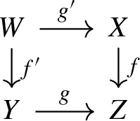
-
(BM3)
\((f\times g)_*(u'\times v')=f_*(u')\times g_*(v')\), \((f\times g)^*(u\times v)=f^*(u)\times g^*(v)\);
-
(PB)
let \(E\rightarrow X\) be a vector bundle of rank \(n+1\), \(q{:}\,\mathbb {P}E\rightarrow X\) its projectivization, \(\mathcal {O}(1)\rightarrow \mathbb {P}E\) tautological line bundle, and \(s{:}\,\mathbb {P}E\rightarrow \mathcal {O}(1)\) its zero section. Then the map
$$\begin{aligned} \sum _{i=0}^n (s^*\circ s_*)^i\circ q^*{:}\,\bigoplus _{i=0}^n A_{*+i-n}(X)\rightarrow A_*(\mathbb {P}E) \end{aligned}$$is an isomorphism;
-
(EH)
let \(p{:}\,V\rightarrow X\) be an affine fibration of rank n. Then \(p^*{:}\,A_*(X)\rightarrow A_{*+n}(V)\) is an isomorphism;
-
(CD)
for \(r,N>0\), let \(W=(\mathbb {P}^N)^r\), with \(p_i{:}\,W\rightarrow \mathbb {P}^N\) being i-th projection. Let also \([X_0{:}\,\cdots {:}\,X_N]\) be homogeneous coordinates on \(\mathbb {P}^N\), \(n_1,\ldots ,n_r\in \mathbb {Z}\), and \(i{:}\,E\rightarrow W\) the subscheme defined by \(\prod _{i=1}^{r}p_i^*(X_N)^{n_i}=0\). Then \(i_*{:}\,A_*(E)\rightarrow A_*(W)\) is injective.

Given an OBM A, we can further define:
-
for any smooth variety Y, set \(A^*(Y):=A_{\dim Y-*}(Y)\). The map \(\Delta _Y^*\circ \times {:}\, A^*(Y)\otimes A^*(Y)\rightarrow A^*(Y)\) defines an associative product on \(A^*(Y)\);
-
for any \(f{:}\,Z\rightarrow Y\), we have the graph morphism \(\Gamma _f=(f,{\text {Id }}_Z){:}\,Z\rightarrow Y\times Z\), which is always a regular embedding. The map \(\Gamma _f^*\circ \times {:}\, A^*(Y)\otimes A_*(Z)\rightarrow A_*(Z)\) defines a \(A^{-*}(Y)\)-module structure on \(A_*(Z)\);
-
for any lci morphism \(f{:}\,Y\rightarrow X\) and arbitrary morphism \(g{:}\,Z\rightarrow X\), we have a Gysin pullback map
$$\begin{aligned} f^!=f^!_g{:}\,A_*(Z)\rightarrow A_*(Z\times _X Y). \end{aligned}$$It coincides with the usual pullback for \(Z=X\), \(g={\text {Id }}_X\). We will also liberally replace f by its pullback \(f'{:}\,Z\times _X Y\rightarrow Z\) in the notations;
-
for any line bundle \(L\rightarrow X\), denote by \(s{:}\,X\rightarrow L\) its zero section. We have a graded homomorphism
$$\begin{aligned} c_1(L):=s^*\circ s_*{:}\,A_*(X)\rightarrow A_{*-1}(X). \end{aligned}$$Moreover, let us consider any vector bundle \(E\rightarrow X\) of rank n together with its projectivization \(q{:}\,\mathbb {P}E\rightarrow X\) and the tautological line bundle \(\mathcal {O}(1)\rightarrow \mathbb {P}E\). Then there exist unique homomorphisms \(c_i(E){:}\,A_*(X)\rightarrow A_{*-i}(X)\) for \(i=\{0,\ldots ,n\}\), called i-th Chern classes, such that \(c_0(E)=1\) and
$$\begin{aligned} \sum _{i=0}^n(-1)^i c_1(\mathcal {O}(1))^{n-i}\circ q^*\circ c_i(E)=0. \end{aligned}$$They satisfy all the usual properties of Chern classes (see [30, Proposition 4.1.15]). For a smooth variety X, the classes \(c_i(E)\) can be realized by elements of \(A^i(X)\);
-
there exists a formal group law \(F_A\in (u+v)+uvA^*(pt)\llbracket u,v\rrbracket \) on \(A^*(pt)\) such that for any \(X\in \mathrm {Sch}_\mathbb {k}\) and two line bundles L, M on X, we have
$$\begin{aligned} c_1(L\otimes M)=F_A(c_1(L),c_1(M)). \end{aligned}$$Since we never consider two OBMs at the same time, we will use multiplicative notation for group laws, and write \(F_A(c_1(L),c_1(M))=c_1(L)\star c_1(M)\).
In [30], Levine and Morel define and study algebraic cobordism theory \(\Sigma _*\) associated to the universal formal group law \((\mathbb {L},F_{\mathbb {L}})\) on the Lazard ring \(\mathbb {L}\). Let us call an OBM Afree if the natural map \(\Sigma _*\otimes _{\mathbb {L}_*}A^*(pt)\rightarrow A_*\) is an isomorphism. For this class of OBMs many properties will follow immediately after establishing them for \(\Sigma _*\).
Example A.2
Chow group functor \({CH}_*\) and the Grothendieck group of coherent sheaves \(K_0\) are free OBMs.
Note that usual Borel–Moore homology is not an OBM, because of the presence of odd-dimensional part. Moreover, even the even-dimensional part fails to be a free OBM, which prevents us from translating results found in [30] in a straightforward way. Still, all of the results we need can be proved in a similar way for the usual Borel–Moore homology. We will thus abuse the language somewhat and allude to it as to a free OBM in the propositions below, giving separate proofs where needed; in the case of omitted proof, we will give a separate reference.
For any reductive group G, free OBM A, and a G-variety X Heller and Malagón-López [19] define equivariant homology groups \(A_*^G(X)\). Roughly speaking, the group G has a classifying space represented by a projective system \(\{EG_N\}_{N \in \mathbb {N}}\) of G-varieties, and we set
For example, if \(G=GL_d\), the varieties \(EG_N\) are just the Grassmanians \({\text {Grass }}^d(d,N)\). Most of the constructions mentioned above for ordinary OBMs can be extended to the equivariant ones.
Example A.3
If \(G=T\) is an algebraic torus of rank d, then by Lemma 1.3 in [52] we have
for some choice of basis \(t_1,\ldots ,t_d\) of the character lattice of T.
Remark A.4
One can observe that in the case of algebraic K-theory we get \(K^T(pt)=\mathbb {Z}[1-t_1^{-1},\ldots ,1-t_d^{-1}]\), which is different from the usual ring of Laurent polynomials \(\mathbb {Z}\llbracket t_1^{\pm 1},\ldots ,t_d^{\pm 1}\rrbracket \). However, the two become isomorphic after passing to completion. One can prove that this happens for any T-scheme X, using the argument in [1, Lemma 3.1] (the author would like to thank Gufang Zhao for this remark).
From now on until the end of appendix, let us fix a free OBM A. Moreover, since we are not concerned with questions of integrality, we also assume that\(A^*(pt)\)contains\(\mathbb {Q}\), so that all A-groups are \(\mathbb {Q}\)-vector spaces. We will often omit homological grading from notations, and write \(A=A_*\), \(A^G=A_*^G\), \(A_G=A^*_G\).
Remark A.5
To the best of author’s knowledge, the notion of oriented Borel–Moore homology theory is not yet fully developed for arbitrary algebraic stacks. However, since all the stacks of interest in our paper are quotient stacks, we usually slightly abuse the notation and write
for any quotient stack [X/G] (see also [19, Proposition 27]).
Proposition A.6
([19, Theorem 26]) Let \(H\subset G\) be a closed subgroup, and X a G-variety. Then there exists a natural isomorphism
where H acts on \(X\times G\) diagonally.
Proposition A.7
([19, Theorem 33]) Let G be a reductive simply connected algebraic group, \(T\subset G\) a maximal torus with normalizer N, \(W=N/T\) the Weyl group, and X a G-variety. Then W acts on \(A^T(X)\), and we have a natural isomorphism
Proposition A.8
Let Z be a non-reduced G-scheme, and denote by \(Z^{red}\) its reduction. Then the pushforward map along the natural embedding
is an isomorphism.
Proof
Follows from the definition of algebraic cobordism theory. For an explicit mention of this fact, see the proof of Proposition 3.4.1 in [30]. \(\square \)
Proposition A.9
(Projection formula) Let \(f{:}\,X\rightarrow Y\) be a G-equivariant projective morphism of smooth varieties, \(\beta \in A^G_*(X)\), and \(\alpha \in A^*_G(Y)\). We have the following identity:
Proof
See [30, Proposition 5.2.1] for non-equivariant version; equivariant proof is completely analogous. \(\square \)
The following proposition holds only for universal OBMs, usual Borel–Moore homology not included.
Proposition A.10
([19, Theorem 20]) Let \(i{:}\,Z\rightarrow X\) be a closed equivariant embedding of G-varieties, and \(j{:}\,U\rightarrow X\) the complementary open embedding. Then the sequence
is exact.
For a G-equivariant vector bundle \(E\rightarrow X\), we define its Euler classe(E) as the top Chern class:
Also, for any regular embedding of smooth varieties \(M\subset N\), let \(T_M N\) be the normal bundle of M in N.
Proposition A.11
(Self-intersection formula) Let \(i{:}\,N\hookrightarrow M\) be a G-equivariant regular embedding of smooth G-varieties. Then
for any \(c\in A^G(N)\).
Proof
Follows from [30, Theorem 6.6.9]. For \(A=H\), see [9, Corollary 2.6.44]. \(\square \)
Given G-equivariant regular embeddings \(j{:}\,P\hookrightarrow N\), \(i{:}\,N\hookrightarrow M\), Whitney product formula applied to the short exact sequence
tells us that
For our purposes, one of the most important pieces of data coming from an OBM is the Gysin pullback. Let us state several compatibility results about it.
Lemma A.12
The following properties of Gysin pullback are verified:
-
(1)
Gysin pullback commutes with composition, that is for any diagram with cartesian squares
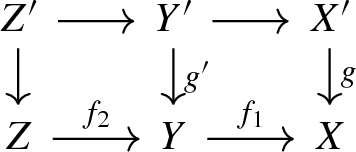
one has \((f_1\circ f_2)_g^!=(f_2)_{g'}^!\circ (f_1)_g^!\), provided that \(f_1\) and \(f_2\) are locally complete intersections;
-
(2)
let \(F{:}\,Y\rightarrow X\), \(G{:}\,X'\rightarrow X\), \(\iota {:}\,Z\rightarrow X\) be morphisms of schemes such that F is lci, G and \(\iota \) are proper, and F and G are transversal. Consider the following diagram, where all squares are cartesian:
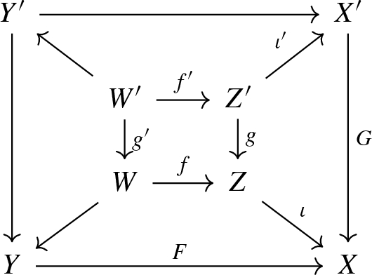
Then we have an equality
$$\begin{aligned}g'_*\circ f'^!_{\iota '}=f_\iota ^!\circ g_*.\end{aligned}$$


Proof
See [30, Theorem 6.6.6(3)] for (1) and [52, Lemma 1.14] for (2). \(\square \)
Proposition A.13
Let \(i{:}\,Y\hookrightarrow X\) be a closed embedding of T-varieties, and \(\{\chi _1,\ldots ,\chi _k\}\subset T^\vee \) a finite set of characters. Suppose that \(X^T\) is not empty, \(X^T\subset Y\), and for any point \(x\in X{\setminus } Y\) its stabilizer under the action of T is contained in \(\bigcup _{i=1}^k{\text {Ker }}(\chi _i)\). Then the pushforward along i induces an isomorphism
Proof
In the interest of brevity, we will abuse the notation and write \(\chi _i\) instead of \(c_1(\chi _i)\). Let us start with surjectivity. By Proposition A.10 we have an exact sequence
Thus it suffices to prove that \(A_*^T(X{\setminus } Y)[\chi _1^{-1},\ldots ,\chi _k^{-1}]=0\). By Lemma 2 in [12], there exists an open subvariety \(U\subset X{\setminus } Y\) and a subgroup \(T_1\subset T\) such that \(U\simeq {\tilde{U}}\times T/T_1\) as T-variety, where \({\tilde{U}}\) is equipped with a trivial action of T. In particular, \(A_*^T(U)\simeq A_*({\tilde{U}})\otimes _{A_*(pt)}A_*^T(T/T_1)\). Because of our hypotheses, one has \(T_1\subset {\text {Ker }}(\chi _i)\) for some i, and thus \(\chi _iA_*^T(U)=0\). We conclude by Noetherian induction. Namely, let Z be the complement of U in \(X{\setminus } Y\). We have the following exact sequence:
By induction \(pA^T(Z)=0\), where p is a monomial in \(\chi _1,\ldots \chi _k\). Therefore \(A^T(X)\) is annihilated by \(\chi _ip\), and thus \(A^T(X{\setminus } Y)[\chi _1^{-1},\ldots ,\chi _k^{-1}]=0\).
It is left to prove injectivity. If \(A=H\), we may already conclude by invoking long exact sequence in homology. Otherwise, we follow an approach found in [4, 2.3, Corollary 2]. First, let us denote
Note that \(Y_\natural \) is non-empty, since \(X^T\subset Y_\natural \). We have the following commutative triangle

where the diagonal arrows are surjective by the first part of the proof. If the horizontal arrow is injective, the same can be said of the map \(A_*^T(Y)[\chi _1^{-1},\ldots ,\chi _k^{-1}]\rightarrow A_*^T(X)[\chi _1^{-1},\ldots ,\chi _k^{-1}]\). Thus, from now on we will assume that \(Y=Y_\natural \).
Let \(U\simeq {\tilde{U}}\times T/T_1\subset X{\setminus } Y\) be as in the proof of surjectivity. Since \(T_1\subset {\text {Ker }}(\chi _i)\) for some i, we get a regular function
It extends to a rational function \(f{:}\,X\rightarrow \mathbb {P}^1_\mathbb {k}\) with the property that \(f(t.x)=\chi _i(t)f(x)\) for any \(x\in X\) and \(t\in T\). In particular, if \(y\in Y\) and \(t\in {\text {Ker }}(\chi _i){\setminus } Stab_T(y)\) this equality becomes \(\chi _i(t)f(y)=f(y)\), so that y belongs to the support of the divisor associated to f. Let us denote this support by D. Thus \(Y\subset D\), and the map \(A_*^T(D)\rightarrow A_*^T(X)\) becomes injective after inverting \(\chi _i\); see [4] for details. We conclude by Noetherian induction on D. \(\square \)
For any commutative ring R and an R-module M, let \(M_{loc}\) be the localized \({\text {Frac }}(R)\)-module \({\text {Frac }}(R)\otimes _R M\).
Theorem A.14
(Localization theorem) Let T be an algebraic torus, \(R=A_*^T(pt)\), X a T-variety, and \(i_T{:}\,X^T\rightarrow X\) inclusion of the fixed point set. Suppose that \(X^T\) is not empty. Then the \({\text {Frac }}(R)\)-linear map
is an isomorphism. Moreover, if X is smooth, then the map
is an isomorphism as well.
Proof
Any action of an algebraic torus has finitely many distinct stabilizers. One can therefore assume that
for some choice of characters \(\chi _1,\ldots ,\chi _k\in T^\vee \). Applying Proposition A.13 to the embedding \(X^T\hookrightarrow X\) and localizing Chern classes of all characters instead of chosen ones, we see that \(i_{T*}\) becomes an isomorphism after localization. In view of Proposition A.11, it remains to prove that if X is smooth, then the Euler class \(e(T_{X^T}X)\) is not a zero-divisor in \(A_*^T(X^T)\). Since the T-action on \(X^T\) is trivial, we can decompose \(T_{X^T}X\) into isotypical components:
where \(p_i\) are non-trivial characters of T, and \(E_i\) are vector bundles on \(X^T\). It suffices to assume \(T_{X^T}X=p_1\otimes E_1\), because Euler class is multiplicative with respect to direct sums. In the case when \(E_1\) is a line bundle, we have
The class \(c_1(p_1)\) is not a zero-divisor by Example A.3, \(c_1(E_1)\) is nilpotent by [30, Remark 5.2.9], therefore \(e(p_1\otimes E_1)\) is not a zero-divisor as well. Finally, the case when rank of \(E_1\) is bigger than 1 can be reduced to the former by using axiom (PB) and the usual technique of Chern roots. \(\square \)
The following proposition describes the behavior of localization map with respect to pullbacks and pushforwards.
Proposition A.15
Let \(f{:}\,X\rightarrow Y\) be a morphism of smooth T-varieties. Assume that the fixed point sets \(X^T\), \(Y^T\) are non-empty, and consider the natural commutative diagram

-
(1)
if f is lci, then \(i_X^*\circ f^*=f_T^*\circ i_Y^*\);
-
(2)
if f is projective, then the following diagram commutes:
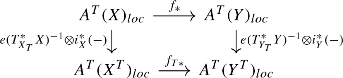

Proof
First claim is obvious, and Proposition A.11 coupled with the localization theorem proves the second claim as well. \(\square \)
Corollary A.16
Under conditions of Proposition A.15(2), we have
for any \(c\in A^T(X)_{loc}\). If, moreover, f is a regular embedding such that \(X^T=Y^T\), then
For the following proposition we fix a reductive group G, and let \(T\subset H\subset P\) be a maximal torus, Levi and parabolic subgroup of G respectively. Denote by W and \(W_H\) the Weyl groups of T in G and H respectively; we also fix a representative \(\sigma \) for each class in \(W/W_H\).
Proposition A.17
Let X be an H-variety, and denote \(Y=G\times _P X\), where the action of P on X is given by the natural projection \(P\rightarrow H\). Then \(Y^T=W\times _{W_H}X^{T}\), and we have a commutative diagram

where \(s{:}\,W\times _{W_H}X^T\rightarrow X^T\) is the projection associated to the choice of representatives \(\sigma \).
Remark A.18
For an arbitrary H-variety X, the action of normalizer \(N_H(T)\) can be restricted to \(X^T\), and thus induces an action of Weyl group \(W_H\) on \(A^T(X^T)\). Moreover, the restriction map \(A^T(X)\rightarrow A^T(X^T)\) can be seen to be \(W_H\)-equivariant. With that in mind, note that even though \(s^*\) depends on the choice of representatives \(\sigma \), its restriction to the \(W_H\)-equivariant part \(A^{T}(X^{T})^{W_H}\), which contains the image of \(i_X^*\), does not.
Proof
First, let us compute T-fixed points of Y. Let (g, x) be a point in \(G\times X\). Then we have:
Therefore \((g,x){\text {mod }} P\) is T-stable iff \((g,x)\in (N_G(T)P)\times (p'.X^{T})/P=W\times _{W_H}X^{T}\), which proves the first claim. Next, let \(i_\xi {:}\,X\hookrightarrow Y\) be the inclusion of the fiber over \(\xi \in G/P\). Note that by definition of \({\text {ind }}_H^G\), it is a right inverse to \(i_e^*\). Therefore, G-equivariance implies that
If we restrict all our structure groups to T and suppose that \(g\in N(T)\), we get
with the action of g on \(A^T(X)\) is as in Proposition A.7. Moreover, we have the following commutative square

since the action of g on \(A^T(X^T)\) is just the restriction of the action above. Finally,
for all \(c\in A^H(X)\), and the second claim follows. \(\square \)
Remark A.19
The same proof as above shows that \((G\times _P X)^T=W\times _{W_H}X^{T}\) for a P-variety X.
Rights and permissions
Open Access This article is licensed under a Creative Commons Attribution 4.0 International License, which permits use, sharing, adaptation, distribution and reproduction in any medium or format, as long as you give appropriate credit to the original author(s) and the source, provide a link to the Creative Commons licence, and indicate if changes were made. The images or other third party material in this article are included in the article’s Creative Commons licence, unless indicated otherwise in a credit line to the material. If material is not included in the article’s Creative Commons licence and your intended use is not permitted by statutory regulation or exceeds the permitted use, you will need to obtain permission directly from the copyright holder. To view a copy of this licence, visit http://creativecommons.org/licenses/by/4.0/.
About this article

Cite this article
Minets, A. Cohomological Hall algebras for Higgs torsion sheaves, moduli of triples and sheaves on surfaces. Sel. Math. New Ser. 26, 30 (2020). https://doi.org/10.1007/s00029-020-00553-x
Published:
DOI: https://doi.org/10.1007/s00029-020-00553-x