

Abstract
We propose a variation of the Guiol–Machado–Schinazi (GMS) model of evolution of species. In our version, as in the GMS model, at each birth, the new species in the system is labeled with a random fitness, but in our variation, to each extinction event is associated a random threshold and all species with fitness below the threshold are removed from the system. We present necessary and suficient criteria for the recurrence and transience of the empty configuration of species; we show the existence of a long time limit distribution of species in the system, and present necessary and suficient criteria for the finiteness of the number of species in that distribution. There is a remarkable symmetry between both sets of criteria. We also highlight fundamental differences between ours and the GMS model, putting them in different universality classes.
Export citation and abstract BibTeX RIS
1. Introduction
In a seminal paper, Bak and Sneppen [1] have proposed a simple model of evolution of species, which has inspired a wealth of studies in several areas of knowledge, including physics, biology and mathematics. In [1], species are identified with sites in a circular 1d grid, and their evolution are described through a dynamics on their fitnesses, which at each step replaces the current minimal fitness along with neighboring current fitnesses at the grid with fresh, independent fitnesses sampled from the standard uniform distribution.
In the mathematics literature, there are few rigorous results concerning the long term behavior of the Bak–Sneppen system. Noteworthy are papers of Meester and Znamenski [2, 3], which derive information on the asymptotic fitness distribution of the model.
Guiol, Machado and Schinazi [4] proposed a different, if somewhat similar dynamics, describing the evolution (in discrete time, as in [1]) of species who independently appear at each time step with probability p, and are assigned a fitness sampled from the uniform distribution on [0, 1]. Extinction occurs at each time step, also independently and with probability 1 − p, whenever there is at least one species present at the corresponding time, in which case the one with the least fitness is removed from the system. Note that the rule to 'kill the least fit' is a common feature with [1]; however, the local interactions of the Bak–Sneppen system are absent. In [4] it was proved that species fitnesses are asymptotically uniformly distributed in (fc, 1), where fc = (1 − p)/p, a similar result to Meester and Znamenski's.
Several extensions and generalizations of the GMS model were subsequently introduced and studied, as in Ben-Ari et al [5], Michael and Volkov [6], Bertacchi et al [7] and Grejo et al [8]. Further, Guiol et al [9] proposed a variation of the model, where the evolution is given in continuous time. See also Formentin and Swart [10] for a closely related model with a different motivation. We refer to this literature for further discussion of the models and results.
We consider here a variation of the GMS model [9] in which, as in that model, new species are born at a given rate, and at possibly another rate we have extinction of species. For each new species in the system, we associate a positive random number, chosen from a distribution F⋆. We call this random number the fitness of the species. So far, the setting is the same as(or quite similar to the one) in [9].
Our variation is (more markedly) related with the extinction events. At the time of each such event, we have a positive threshold random variable, with distribution F†, and all species with fitness below this threshold at that time, if any, get extinct.
We believe this is a natural variation of the GMS model, when we consider extinction of species in the natural world produced by major events such as abrupt habitat change, where conceivably each species might be affected according to its own aptitude to face the new challenge, irrespective of other species.
The random fitnesses and the random thresholds are independent of each other and of everything else in the process. We assume F⋆ is continuous on  ; so, in particular, we can and will identify each species with its fitness. We also assume, for simplicity, that F⋆ and F† have unbounded support.
Let Π⋆ and Π† be independent Poisson point processes in  with rates λ⋆ and λ†, respectively. Define
  as the set of birth time instants of a new species in the system, define
  as the instants of time in which there is an extinction event. These sequences represent the points in the Poisson processes and are indexed in increasing order. At each time Ti ∈ Π⋆ we assign to the newly appeared species the fitness Xi, drawn from F⋆, and to each time Sj ∈ Π† we associate the threshold Yj from distribution F†.
Given a locally finite subset A of  , let ηt = {ηt(s), s ⩾ t} denote our evolution model starting from A at time t. So, at initial time
  , the process has initial configuration ηt(t) = A, and at time s ∈ (t, ∞), the process has the configuration ηt(s) which is composed of all species/fitnesses either of A or that have appeared in the time interval (t, s], and that have survived the events of extinction in [t, s], i.e. species whose fitnesses are greater than the highest threshold drawn in events of extinction in [t, s] after their birth.
Notice that as long as A does not depend on t, neither does the distribution of ηt, so below we will often restrict to η0.
Figure 1 simulates a realization of the process ηt in the time interval [t, s]. Each circle represents a species alive in the process and the gray arrow issuing from it represents its life time. Observe that the position of each species in relation to the vertical axis is given by its fitness. The three black circles represent the configuration of the process at time t. The six gray circles represent the species that were born in the time interval [t, s]; the positions that they occupy represent the respective instants of time they were born (horizontal axis) and the fitnessess that were drawn to them (vertical axis). The four withe circles represent the species that survived the extinction events and are alive at the time s. Finally, each extinction threshold is represented in figure 1 by black stars.
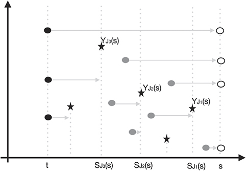
Figure 1. Possible configuration of process ηt in the time interval [t, s].
Download figure:
Standard image High-resolution image1.1. Preliminary comparison to the GMS model
Before going to our results, let us briefly discuss preliminarily how our model compares with the GMS model (of [9]). One difference is that we have fitnesses in  rather than [0, 1], but this is not important, or rather just a matter of changing the fitness scale. More importantly, our thresholds are also supported in
  , and one might point out that the model makes sense for a bounded threshold distribution. In this case, we would allow for another feature missing from our model and present in the GMS model, namely, the eternal species. However, this would be a trivial phenomenon in our model (any species with fitness above the upper bound of the threshold distribution would automatically be eternal, and none below that upper bound). The most interesting comparison between the models would be thus our model in the above formulation (both fitnesses and extinction thresholds unboundedly supported) and the GMS model below the critical fitness value (for the occurrence of eternal species).
In terms of recurrence of the empty state and finiteness of the number of species in the limiting distribution of species fitnesses, the latter model is known to show recurrence and infinitely many species in the limit. As we will see below our model may show different behavior in both this respects, depending on F⋆ and F†, but there are choices, such as F⋆ = F†, for which both models behave the same in both these respects. It is then natural to ask whether our model with F⋆ = F† behaves the same as the GMS model below the critical fitness value at other fundamental levels, thus putting them in a sense in the same universality class. But we find that the models behave fundamentally differently, regarding a third issue, in this case as well; see remark 2.14 below.
One other distinguishing aspect, a more technical one, is that the GMS model may be described in terms of a spatial birth-and-death process. Ours cannot. In particular, the number of species present at time t, which performs an ordinary birth-and-death process on  in the GMS model, with jumps only of size 1 in any direction, does not do so in our case, where there may be jumps larger than 1 towards 0, and is not even Markovian. The technical approach of analysis required in our case is thus quite different from the ones of the literature related to [9], as will become clear below.
1.2. Records.
Elaborating on the latter point above, our technical approach to treat our model relies substantially on classical record theory. This is a topic of much recent interest in theoretical physics, with an effort in modeling phenomena such as record temperatures in global warming, or record prices in the stock market, and other examples; see [11, 12], and references therein. Some of these phenomena depart from the classical i.i.d. setting in that the underlying sequence of random variables have a time trend, and are thus not identically distributed, or exhibit correlations; these are the settings analyzed in [11, 12] and other recent work.
The questions we ask about our model involve records as follows. As regards recurrence of the empty state, we have returns to that state whenever we find extinction points above the staircase formed by records of fitness of succesive species, as they appear going forward in time. The other issue is finiteness of the limiting configuration of species fitnesses, and this is given by the fitnesses of the species appearing above the staircase of records of extinction thresholds, going backwards in time. We defer further details for the coming sections of this paper. The description of the record staircase in both cases follows from the classical theory, since we specify i.i.d. fitnesses and extinction thresholds, and Poisson point processes for the birth and extinction times. It makes sense however to consider time dependent and/or correlated specifications, as those of [11, 12], in the context of our model, which might yield interesting extensions of our results.
2. Results
We derive three kinds of results. First, criteria for recurrence and transience of the empty configuration in η0; see theorem 2.1 below; they are obtained from the analysis of a Poisson process of records. Second, we derive the existence of a limit distribution for η0(s) as s → ∞; see theorem 2.2 below. Finally, we derive criteria for finiteness and infiniteness of the number of species present in the limit distribution; see theorem 2.3 below; curiously, the Poisson process of records of the recurrence and transience issue appears here as well, but in reverse. The behavior of  at the origin plays a determinant role in the first result, and thus, in reverse, so does that of
  in the third one; as usual, for * = ⋆ and †,
  , and
, and  indicates the (right-continuous) inverse of
  , namely

For the latter result we need to assume that F† is continuous. Proofs are deferred to the last section.
Let us define the functions  by
by
For birth events denote by Ik the record indexes and by  the record values, as follows: I1 ≐ 1; and for k ⩾ 1

Proposition 2.1. (Proposition 4.11.1, Resnick [13]). The record values  form a Poisson point process in
  with intensity measure ∫BR⋆(dx),
  .
.
The next result refines the previous one.
Proposition 2.2. Let  be the time of the kth record and denote by
  the interval between two consecutive records. Then,
  is a Poisson process in
  with intensity measure
Proposition 2.3. The set of points  is a Poisson process in
  , denoted by
  , with intensity measure
To study recurrence and transience, we will build a ladder of records using the process of births and the fitness associated to each species. Let us denote the random region above each step of the ladder by  , and the region above the full ladder is denoted by D, namely, for k ⩾ 1
Let Λ ≐ μ†(D),  , and
, and  . Observe that M counts the number of extinction events in D—as noted in Sub section 1.2, these extinction marks generate empty configurations, with no species present at and immediately after their corresponding times3. Given D, M has a Poisson distribution with mean Λ (because
  is a Poisson process), so

Here we allow Λ = ∞, in which case M = ∞ a.s. It may be checked, from ergodicty considerations, that {Λ = ∞} is a trivial event, and, thus, so is {M = ∞}.
Remark 2.4. Define  by
by  . From the definition of μ† in proposition 2.3, we have

Note that ![$\mathbb{E}\left[M\right]=\mathbb{E}\left[\mathbb{E}\left[M\vert {\Lambda}\right]\right]=\mathbb{E}\left[{\Lambda}\right]$](https://content.cld.iop.org/journals/1751-8121/53/19/195601/revision2/aab7cfdieqn33.gif) and we may use Campbell's formula (see proposition 2.7 in [14]) and (2) to find
and we may use Campbell's formula (see proposition 2.7 in [14]) and (2) to find

2.1. Recurrence/transience of η0
We start by discussing the a.s. finiteness of M. Define the functions  and ψ: [0, 1] → [0, 1] by
and

By monotone convergence, we have that
Proposition 2.6. The following statements are equivalent:
- (a)ϕ(∞) < ∞;
- (b)
 ;
; - (c);
- (d) is integrable at the origin;
- (e)ψ(s−1) is integrable at infinity.
![$\mathbb{E}\left[M\right]{< }\infty $](https://content.cld.iop.org/journals/1751-8121/53/19/195601/revision2/aab7cfdieqn36.gif)

Definition 2.7. Let ϒ = {s ⩾ 0 : η0(s) = ∅} denote the set of times where the species configuration is empty; in other words, ϒ is the set of times where there is no species in the system. ϒ is readily seen to a.s. consist of a collection {[aj, bj), j ⩾ 1}, either finite or infinite, of disjoint finite intervals. Let ϒ' = {aj, j ⩾ 1} be the collection of left endpoints of such intervals, correspondings to the times where the species configuration freshly becomes empty. We have that  , where
  is the projection of
  on the time axis. (However, as pointed out above,
  a.s.; see footnote on page 5.)
The process η0 is said to be transient if ϒ is a.s. a bounded set. On the other hand, if ϒ is a.s. an unbounded set, then we say that η0 is recurrent.
We point out that, since the set of fitness record times  is unbounded, we have that ϒ/ϒ' is bounded if and only if
  is bounded.
Theorem 2.1. The process η0 is transient if
and recurrent otherwise.
Example 2.8. Suppose that (Xi) and (Yj) are exponentially distributed with parameter α⋆ and α†, respectively. Then,
By proposition 2.6, if α† ⩽ α⋆, then M = ∞ a.s., and from theorem 2.1, η0 is recurrent. If α† > α⋆, then η0 is transient. We may compute the distribution of Λ and M in this case (it will come in handy below), as follows: by 2, ![$\mathbb{E}\left[{\mathrm{e}}^{-t{\Lambda}}\right]=\mathbb{E}\left[{\mathrm{e}}^{-{\sum }_{k{\geqslant}1}t.{h}_{{\dagger}}\left({X}_{{I}_{k}},{\Delta}{T}_{{I}_{k}}\right)}\right]$](https://content.cld.iop.org/journals/1751-8121/53/19/195601/revision2/aab7cfdieqn44.gif) and using the characterisation of a Poisson process via its Laplace functional (see theorem 3.9 on page 23 of [14])
and using the characterisation of a Poisson process via its Laplace functional (see theorem 3.9 on page 23 of [14])
By proposition 2.5, ![$\mathbb{E}\left[{\mathrm{e}}^{-tM}\right]={\left(\frac{1-p}{1-p{\text{e}}^{-t}}\right)}^{r}$](https://content.cld.iop.org/journals/1751-8121/53/19/195601/revision2/aab7cfdieqn45.gif) , where
, where  and
and  . Hence, Λ follows the gamma distribution with parameters r and β, and M follows the negative binomial distribution with parameters r and p.
2.2. Existence and in/finiteness of a long time limit distribution.
We now establish the existence of a limit distribution for η0(s) as s → ∞. Remarkably, a ladder construction based on a record process comes up here as well, entirely parallel to that of subsection 2.1, with births and extinctions swapping roles. For that to hold we need however to assume that F† is continuous. The ladder construction then immediately yields necessary and sufficient criteria for the almost sure in/finiteness of the number of species present in the limit distribution, identical to those for transience/recurrence of η0, except that the symbols ⋆ and † swap roles.
As a preliminary, we will use the process of extinctions and the associated thresholds to build a ladder of records, much as in subsection 2.1. We define the kth record index Jk and the record value  as follows: J1 ≐ −1 and; for k ⩾ 1

Again by proposition 4.11.1 in [13], we get that the  form a Poisson point process in
  with intensity measure ∫BR†(dx),
  .
.
Denote by  the time of the kth record, and by
  the time span between two consecutive records. Similarly as in subsection 2.1, we have the following results.
Proposition 2.9. The points  form a Poisson point process in
  with intensity
Proposition 2.10. The points  form a Poisson point process in
  ,
, ![${\mathbb{R}}_{-}=\left(-\infty ,0\right]$](https://content.cld.iop.org/journals/1751-8121/53/19/195601/revision2/aab7cfdieqn58.gif) , denoted by
, denoted by  , with intensity
We thus have our ladder of thresholds; denote the region above each step by
We state our existence result.
Theorem 2.2. η0(t) converges in distribution to  as t → ∞, where
Remark 2.11. The topology for weak convergence is the usual one in the context of point processes. Our proof indeed makes use of a coupling to a sequence of processes for which the convergence is a strong one, and follows by monotonicity.
Next, we address the issue of finiteness of the number of species in  . For each k ⩾ 0, let

Let also Σ ≐ μ⋆(E);  . We may use Campbell's formula to find
Note that N is the number of birth events above the threshold ladder. Also, note that E has a parallel structure to that of the D ladder of subsection 2.1; the random variables Σ and N are parallel to Λ and M in that same subsection. Thus, we get parallel results, once we exchange the roles of  and
and  .
.
From theorem 2.2, the number of species present in the limit distribution  , denoted by
  , is
, is

It is enough to consider the finiteness of N. From the parallel situation of subsection 2.1, we get the following results. For t > 0
Setting
and

we have
Proposition 2.12. The following statements are equivalent:
- (a);
- (b);
- (c).
- (d) is integrable at the origin;
- (e) is integrable at infinity.

![$\mathbb{E}\left[N\right]{< }\infty $](https://content.cld.iop.org/journals/1751-8121/53/19/195601/revision2/aab7cfdieqn69.gif)


Theorem 2.3. The number of species in the limit distribution,  , is finite if
and infinite otherwise.
Example 2.13. Let (Xi) and (Yj) be as in example 2.8. We have then
By the theorem 2.3, if α⋆ ⩽ α†, then  a.s. If α⋆ > α†, then
  a.s.; let us find its distribution. We can show that, as in example 2.8, N follows the negative binomial distribution with parameters
  and
and  . From the joint distribution of (N0, Σ0), discussed in the proof of theorem 2.3 below, we have that N0 follows the negative binomial distribution with parameters 1 and
  . It may be checked that N0 and N are independent, and we find from (5) that
  follows the negative binomial distribution with parameters
  and
and  .
.
Remark 2.14. We might label the case of ∞ in both criteria in theorems 2.1 and 2.3 as null recurrent. This is of course the case when F⋆ = F†, which then becomes a natural candidate for comparison with the GMS model below the critical point, which also is recurrent and has infinitely many species in its limiting distribution, as anticipated in subsection 1.1, and is thus null recurrent in the same way. However, as we briefly discuss below—see remark 3.1—, in this case the models are different in another fundamental level, namely the behavior of Nf, the number of species in the limiting distribution with fitness below f, as f → ∞ (in our setting; in the setting of [9], the limit should be taken as f ↑ fc). While for the GMS model the suitably rescaled object converges in distribution as the scale parameter vanishes to a nontrivial distribution—see theorem 1.2 of [10]—, we have a law of large numbers type of convergence to a constant in our model. In the terms proposed in the latter reference, this puts the two models in different universality classes.
3. Proofs
Our proofs of propositions 2.2 and 2.3 use definition 5.3 (K-marking process), as well as theorem 5.6 (Marking theorem) in [14].
Proof of Proposition 2.2. Conditional on  , the random variables
  are independent of each other and follow the exponential distribution of rate
  . Denote by K⋆(x, B) the following probability kernel: for x ⩾ 0, and B = (s1, s2] ⊂ [0, ∞), let
 ![${K}_{\star }\left(x,\left({s}_{1},{s}_{2}\right]\right)\doteq {\mathrm{e}}^{-{\lambda }_{\star }\overline{{F}_{\star }}\left(x\right){s}_{1}}-{\mathrm{e}}^{-{\lambda }_{\star }\overline{{F}_{\star }}\left(x\right){s}_{2}}$](https://content.cld.iop.org/journals/1751-8121/53/19/195601/revision2/aab7cfdieqn84.gif) , and extend the definition for Borelians B in the usual way.
, and extend the definition for Borelians B in the usual way.
The points  form a K⋆-marking of the Poisson process of proposition 2.1. The result follows by the Marking Theorem (theorem 5.6 of [14]).□
Proof of Proposition 2.3. The random variables  are independent of each other and independent of
  . Then, the points
  form a
  -marking independent of
  , where
  is the measure induced by Y. The result follows again by the Marking theorem. □
Proof of Proposition 2.5. From equations (1) and (2)


In (6) we used the characterisation of a Poisson process via its Laplace functional (see theorem 3.9 on page 23 of [14]), and (7) follows by proposition 2.2.
Integrating the above expression in s, we have
□
Proof of Proposition 2.6. To prove (a) ⇒ (b) note that
Integrating (8) against R⋆(dx) we get,

If ϕ(∞) < ∞, by monotone convergence theorem, limt↓0 ϕ(t) = 0. Then,

and, on the other hand,
To prove (b) ⇒ (a) suppose ϕ(∞) = ∞. By (9), ϕ(t) = +∞ for each t > 0. Then,
By contradiction we get (b) ⇒ (a).
Since trivially (c) ⇒ (b), we have from the above that (c) ⇒ (a).
To show that (a) ⇒ (c), we will change variables. Let  , so
, so  . From this and (4),
  . Making u = e−y, we find that
where the second equality is quite clear if F⋆ is strictly increasing, but holds in general (see e.g. the [15] for a discussion and justification).
If ϕ(∞) < ∞, then dominated convergence yields

Since
we get that

Solving the integral,
and from (10)

We may thus find δ ∈ (0, 1) such that λ†ψ(u) ⩽ λ⋆u for each u ∈ (0, δ). Thus,

Thus, since also ψ(u) ⩽ 1, we have
Rewriting (3) in terms of ψ, we have

and the finiteness of the latter expression establishes that (a) ⇒ (c).
(c) ⇔ (d) follows readily from (11). To prove (d) ⇔ (e) make the following substitution
and we can rewrite ![$\mathbb{E}\left[M\right]$](https://content.cld.iop.org/journals/1751-8121/53/19/195601/revision2/aab7cfdieqn95.gif) as
as
Note that
as a consequence
□
Proof of Theorem 2.1. By proposition 2.6, if  , then M = ∞ a.s. Since
  is a.s. finite for every k ⩾ 1, we have that
  is a.s. unbounded, and thus so is ϒ' and ϒ.
If  , then by proposition 2.6, we have that a.s. M < ∞, and thus
  is bounded, and thus so is ϒ' and ϒ, as follows from what has been pointed out at the end of definition 2.7 above. □
Proof of Theorem 2.2. By the homogeneity of the model, the process ηt = {ηt(t + s) : s ⩾ 0} has the same distribution for each  . In particular,

where A is a locally finite subset of [0, ∞). Let  be an increasing sequence in
  such that tl → ∞ as l → ∞ and A as above; take a sequence of processes
  such that
  , l ⩾ 1. Define the sequence
  by
by
where  , and the union
  above is empty if
  . Note that
  is an increasing sequence with
  as l → ∞. Thus, the sequence
  is increasing and
  , with
Define the sequence  by
by
By proposition 2.9,  as k → ∞, since R†(x) < ∞ for every x > 0 and R†(x) → ∞ as x → ∞. Thus,
  is an increasing sequence with
  , since
  as l → ∞. Therefore,
  is a decreasing sequence and
  . Because
  for each l ⩾ 1, we have that
  , and notice that the limit does not depend on the choice of
  . Thus
  a.s., and, by (12),
  in distribution as t → ∞.□
Proof of Proposition 2.12. The proof is analogous to that of proposition 2.6, using the same ideas, and changing the roles of  and
and  . □
. □
Proof of Theorem 2.3. N0 has a Poisson distribution with parameter Σ0. Since Σ0 = μ⋆(E0) = λ⋆(0 − S−1) ∼ exponential (λ†/λ⋆), we have that ![$\mathbb{E}\left[{N}_{0}\right]=\mathbb{E}\left[{{\Sigma}}_{0}\right]={\lambda }_{\star }/{\lambda }_{{\dagger}}{< }\infty $](https://content.cld.iop.org/journals/1751-8121/53/19/195601/revision2/aab7cfdieqn128.gif) , and thus N0 < ∞ a.s.
, and thus N0 < ∞ a.s.
By (5) and proposition 2.12, if  , then N < ∞ a.s., and thus
  a.s. Otherwise, N = ∞ a.s., and we have
  a.s. □
Remark 3.1. As a final remark, we argue in a few brief steps that, as pointed out in remark 2.14 above, when F⋆ = F† = F, then Nf, the number of species in the limiting distribution with fitness below f, when properly rescaled, converges (a.s.) to a nontrivial constant. First, by the above construction of the limiting distribution of species fitnesses, it is enough to consider the intensity measure of the region bounded by the ladder of records, the x-axis and the horizontal line through (0, f). This in turn may be readily written as

where  is a Poisson point process on
  of intensity measure ∫BR(dx),
  , with
  , and
, and  are i.i.d. standard exponential random variables. Clearly, the first term on the right hand side of (13), when scaled by R(f), converges to 1 almost surely as f → ∞, by the law of large numbers. We leave as an exercise to check, using well known properties of Poisson point processes such as
  , that the second term, when scaled by R(f), vanishes almost surely as f → ∞; indeed, without scaling, it is stochastically bounded uniformly by a non degenerate random variable; we immediately get convergence to 0 in probability of the scaled quantity, and a closer look reveals that this can be strengthened to a.s. convergence.
Footnotes
- *
Research supported by CAPES; PNPD-CAPES; CNPq 311257/2014-3; FAPESP 2017/10 555-0
- 3
But there may be, and indeed there a.s. are, extinction marks generating an empty configuration which appear below D.