Exploring Light Sterile Neutrinos at Long Baseline Experiments: A Review

1
Dipartimento Interateneo di Fisica “Michelangelo Merlin”, University of Bari, Via Amendola 173, I-70126 Bari, Italy
2
Istituto Nazionale di Fisica Nucleare (INFN), Sezione di Bari, Via E. Orabona 4, I-70126 Bari, Italy
Universe 2020, 6(3), 41; https://doi.org/10.3390/universe6030041
Submission received: 10 January 2020
/
Revised: 27 February 2020
/
Accepted: 28 February 2020
/
Published: 7 March 2020
(This article belongs to the Special Issue Neutrino Oscillations)
Abstract
:Several anomalies observed in short-baseline neutrino experiments suggest the existence of new light sterile neutrino species. In this review, we describe the potential role of long-baseline experiments in the searches of sterile neutrino properties and, in particular, the new CP-violation phases that appear in the enlarged 3 + 1 scheme. We also assess the impact of light sterile states on the discovery potential of long-baseline experiments of important targets such as the standard 3-flavor CP violation, the neutrino mass hierarchy, and the octant of .
1. Introduction
More than twenty years ago, groundbreaking observations of neutrinos produced in natural sources (sun and Earth atmosphere) provided the first evidence of neutrino oscillations and established the massive nature of neutrinos [1,2,3,4,5]. Subsequently, the neutrino properties have been clarified by experiments using man-made sources of neutrinos (nuclear reactors and accelerators). The two simple 2-flavor descriptions adopted in the beginning to describe disjointly the solar and the atmospheric neutrino problems have been gradually recognized as two pieces of a single picture, which is presently considered as the standard framework of neutrino oscillations. We recall that in the 3-flavor scheme there are three mass eigenstates with masses [and therefore two independent mass-squared splittings (, )], three mixing angles , and one CP-phase . The neutrino mass hierarchy (NMH) is defined to be normal (NH) if or inverted (IH) if .
Despite its huge success, the standard 3-flavor scheme does not need to constitute an exact description. As a matter of fact, several anomalies have been found in short baseline experiments (SBL), which cannot be explained in the 3-flavor scenario (for reviews on this subject, see [6,7,8,9,10,11,12,13,14,15]). The indications come from the accelerator experiments LSND [16] and MiniBooNE [17], and from the so-called reactor [18] and Gallium [19,20] anomalies. Constraints on light sterile neutrinos have been derived also by the long-baseline (LBL) experiments MINOS and MINOS+ [21,22], NOA [23], and T2K [24]; by the reactor experiments Daya Bay [25],1 DANSS [27], NEOS [28], Neutrino-4 [29], PROSPECT [30], and STEREO [31]; by the atmospheric neutrino data collected in Super-Kamiokande [32], IceCube [33,34], and ANTARES [35]; and by solar neutrinos [36,37,38].
The two standard mass-squared splittings and are too small to give rise to detectable effects in SBL setups. Therefore, one new much bigger mass-squared difference must be invoked to explain the SBL anomalies. The new hypothetical mass eigenstate must be supposed to be sterile, i.e., a singlet of the standard model gauge group. Several new and more sensitive SBL experiments are underway to put under test such an intriguing hypothesis (see the review in [39]), which, if confirmed would provide a concrete evidence of physics beyond the standard model. In the minimal extension, the so-called scheme, only one sterile species is introduced. In this scenario, one assumes the existence of one mass eigenstate weakly mixed with the active neutrino flavors () and separated from the standard mass eigenstates by a difference. In the 3 + 1 framework, there are six mixing angles and three (Dirac) CP-violating phases. Therefore, in the eventuality of a discovery of a light sterile species, we would face the daunting task of nailing down six new properties (three mixing angles, two CP-phases, and the mass-squared splitting ). Several global analyses performed in the 3 + 1 scheme [12,13,14,15] show that the fit noticeably improves with respect to the standard 3-flavor case. However, all such analyses evidence an internal tension between different classes of experiments. More specifically, a tension among the joint disappearance data ( and ) and the appearance data () is present and has become stronger in the latest analyses. This has led to increasingly lower values for the best fit of and especially , which currently are close [13] to and , and are slightly smaller than the values that we have taken as a benchmark in this review ().
The scenario naturally implies sizeable effects at short distances, where the oscillation factor (L being the baseline and E the neutrino energy) is of order one, and the typical dependency of the signal is expected. However, we stress that sterile neutrinos can leave imprints also in other (non-short-baseline) kinds of experiments, where they have an impact in a more subtle way. In the atmospheric neutrinos, as first shown in [40], at O(TeV) energies, a novel Mikheyev-Smirnov-Wolfenstein (MSW) resonance arises, which produces sizeable modifications of the zenith angle distribution. In the solar sector, a non-zero mixing of the electron neutrino with (parameterized by the matrix element ) leads to detectable deviations from the unitarity of the subsystem [36,37] (see also [38]).
Light sterile neutrinos can produce observable effects also in the long-baseline (LBL) accelerator experiments. We recall that such setups, when working in the (and ) appearance channel, are able to identify the 3-flavor CP violation (CPV) induced by the standard CP-phase . This sensitivity is strictly related to the circumstance that at long distances the conversion probability contains an interference term (which is unobservable at SBL experiments) among the oscillations induced by the solar mass-squared difference and those driven by the atmospheric one. As first shown in [41], if sterile neutrinos participate in the oscillations, a new interference term arises in the conversion probability, which contains one additional CP-phase. Notably, the new genuine 4-flavor interference term is expected to have an amplitude similar to that of the standard 3-flavor interference term. Hence, the detection of the new interference term opens the concrete opportunity to explore the enlarged CPV sector implied by the presence of sterile neutrino species. It should be stressed that, in both the 3-flavor and 4-flavor frameworks, the CP-phases cannot be detected in SBL experiments, since in these setups the two standard frequencies and have a negligible impact. Therefore, the SBL and LBL facilities are synergic in searches of the 3 + 1 framework (and of any other framework that involves more than one sterile state).
These basic observations provide the motivation for writing the present review, in which we discuss the physics potential of the future LBL experiments in the presence of a hypothetical light sterile neutrino. The subject is very active as testified by the numerous works about DUNE [42,43,44,45,46,47,48], T2HK [48,49,50], and T2HKK [48,51]. Other studies on the impact of light sterile neutrinos in LBL setups can be found in [52,53,54,55,56,57,58,59,60]. We underline that, while this review deals with charged current interactions, one can obtain valuable information on active-sterile oscillations parameters also from the analysis of neutral current interactions (see [21,22,23,24] for constraints from existing data and [47,61] for sensitivity studies of future experiments). Finally, we would like to stress that our review is limited to the oscillation phenomenology, although light sterile neutrinos may have an impact also on non-oscillation searches. We mention the studies focused on the leptonic decays of charged leptons and mesons [62], the beta decay [63], and the neutrinoless double-beta decay [64,65].
The review is organized as follows. In Section 2, we present the theoretical framework and introduce the basic formulae for the 4-flavor and transition probabilities. In Section 3, we provide the specifications of the three setups DUNE, T2HK, and ESSSB, which we use in the numerical simulations. In Section 4, we describe the details of the statistical method that we use for the analysis. In Section 5, we discuss the sensitivity to the LBL experiments to the NMH in the presence of a light sterile neutrino. In Section 6, we describe the sensitivity to CPV and, in Section 7, we study the ability to reconstruct the CP phases. In Section 8, we present an important degeneracy issue, which affects the reconstruction of the octant of in the 3 + 1 scheme. We trace the conclusions in Section 9. Appendix A contains the analytical treatment of the matter effects relevant for LBL experiments in the 3 + 1 scheme.
2. Theoretical Framework
In the presence of a sterile neutrino, the flavor () and the mass eigenstates () are connected by a unitary matrix
with () denoting a real (complex) rotation of a mixing angle , which incorporates the submatrix
in the sub-block. To simplify the notation, we define
The parameterization in Equation (1) enjoys some useful properties: (i) The 3-flavor matrix is recovered by setting . (ii) For small values of the mixing angles , , and , one has , , , and , with a clear physical interpretation of the three mixing angles. (iii) The leftmost positioning of the matrix implies that the transition probability in vacuum is independent of and of the associated CP phase (see [41]).
For clearness, we confine the discussion to the case of propagation in vacuum. We address the impact of matter effects in Appendix A. As first shown in [41], the transition probability can be written as the sum of three contributions
The first term, which is positive-definite, depends on the atmospheric mass-squared splitting and provides the leading contribution to the probability. It takes the form
where is the atmospheric oscillating factor, L and E being the neutrino baseline and energy, respectively. The other two contributions in Equation (4) arise from the interference of two different frequencies and are not positive-definite. Specifically, the second term in Equation (4) is related to the interference of the solar and atmospheric frequencies and can be written as
where we introduce the ratio of the solar over the atmospheric mass-squared splitting, . We recall that at the first (second) oscillation maximum one has (). The third contribution in Equation (4) appears as a new genuine 4-flavor effect, and is related to the interference of the atmospheric frequency with the new high frequency induced by the presence of the fourth mass eigenstate. This term can be written in the form [41]
From Equations (5)–(7), we see that the conversion probability depends on (besides the large mixing angle ) three small mixing angles: the standard angle and two new angles and . We note that the values of such three mixing angles (estimated in the 3-flavor scenario [66,67,68] for , and in the 4-flavor framework [12,13,14,15] for and ) are similar and one has (see Table 1). Therefore, one is naturally induced to consider these three angles as small quantities having the same order of magnitude . We also notice that, since , it can be considered of order . From inspection of Equations (5)–(7), we derive that the first (leading) contribution is of the second order, while the two interference terms are both of the third order. However, we underline that, differently from the standard interference term in Equation (6), the new sterile-induced interference term in Equation (7) is not proportional to but to ; hence, it is not enhanced at the second oscillation maximum. Because of this feature, as our numerical simulations will confirm, the performance of ESSSB in the 4-flavor scenario is not as good as that of DUNE and T2HK, which work around the first oscillation maximum.
Before closing this section, we underline the fact that the conversion probability in vacuum is independent of the third mixing angle and of the related CP-phase . As shown in Appendix A, this conclusion does not hold anymore in the presence of matter. In practice, as we discuss in the subsequent sections, the CP-phase can be probed only in DUNE, which among the planned LBL experiments, is the most sensitive to the matter effects.
3. Description of the Experimental Setups
3.1. DUNE Setup
Hosted at Fermilab, DUNE is a new-generation long-baseline neutrino oscillation experiment which will play an important role in the future neutrino roadmap to discover the fundamental properties of neutrino [69,70,71,72,73]. DUNE will be composed of three major ingredients: (a) an intense (∼ megawatt), broad-band neutrino beam at Fermilab; (b) a high-precision near neutrino detector just downstream of the neutrino source; and (c) a massive (∼ 40 kt) liquid argon time-projection chamber (LArTPC) far detector hosted deep underground at the Sanford Underground Research Facility (SURF) 1300 km away in Lead, South Dakota. We assume a fiducial mass of 35 kt for the far detector in our simulations, and consider the detector properties which are given in Table 1 of Reference [74]. Concerning the beam, we consider a proton beam power of 708 kW with a proton energy of 120 GeV, which can deliver protons on target on 230 days per calendar year. In our simulation, we have taken the fluxes which were estimated assuming a decay pipe length of 200 m and 200 kA horn current [75]. We consider a total run time of ten years for this experiment, which is equivalent to a total exposure of 248 kt · MW · year. We assume that the DUNE experiment would use half of its full exposure in the neutrino mode, and the remaining half in the antineutrino mode. In our simulations, we take the reconstructed neutrino and anti-neutrino energy range to be 0.5–10 GeV. To incorporate the systematic uncertainties, we consider an uncorrelated 5% normalization error on signal and 5% normalization error on background for both the appearance and disappearance channels to analyze the prospective data from the DUNE experiment. We consider the same set of systematics for both the neutrino and antineutrino channels which are also uncorrelated. For both and appearance channels, the backgrounds mostly arise from three different sources: (a) the intrinsic / contamination of the beam; (b) the number of muon events which will be misidentified as electron events; and (c) the neutral current events. Our assumptions on various components of the DUNE set-up are similar to those mentioned in the Conceptual Design Report (CDR) reference design in Reference [70].
3.2. T2HK Setup
The main goal of the long-baseline neutrino program at the proposed Hyper-Kamiokande (HK) detector with a neutrino beam from the J-PARC proton synchrotron is to give a conclusive evidence for leptonic CP-violation in neutrino oscillations induced by the CP-phase in the 3-flavor neutrino mixing matrix. This setup is commonly known as “T2HK” (Tokai to Hyper-Kamiokande) experiment [76,77,78]. To calculate the physics reach of this setup, we closely follow the experimental specifications as described in References [77,78]. The neutrino beam for HK will be produced at J-PARC from the collision of 30 GeV protons on a graphite target. In our simulations, we consider an integrated proton beam power of 7.5 MW × s, which can deliver in total protons on target (p.o.t.) with a 30 GeV proton beam. We assume that the T2HK experiment would use 25% of its full exposure in the neutrino mode which is p.o.t. and the remaining 75% ( p.o.t.) would be used for the antineutrino run. This ensures that we have nearly equal statistics in both neutrino and antineutrino modes to optimize the search for leptonic CP-violation. These neutrinos and antineutrinos will be observed in the gigantic 560 kt (fiducial) HK water Cherenkov detector in the Tochibora mine, located 8 km south of Super-Kamiokande and 295 km away from J-PARC. The neutrino beamline from J-PARC is designed to produce an off-axis angle of ∼ at the proposed HK site and, therefore, the beam peaks at the first oscillation maximum of 0.6 GeV to enhance the physics sensitivity. This off-axis scheme [79] gives rise to a neutrino beam with a narrow energy spectrum which substantially reduces the intrinsic contamination in the beam and also the background deriving from neutral current events. In our analysis, we consider the reconstructed neutrino and antineutrino energy range of 0.1–1.25 GeV for the appearance channel. In case of disappearance channel, the assumed energy range is 0.1–7 GeV for both the and candidate events. We match all the signal and background event numbers following Tables 19 and 20 of Reference [77]. The systematic uncertainties play an important role in estimating the physics sensitivity of the T2HK setup. Following Table 21 of Reference [77], we consider an uncorrelated normalization uncertainty of 3.5% for both appearance and disappearance channels in neutrino mode. In the case of antineutrino run, the uncorrelated normalization uncertainties are 6% and 4.5% for appearance and disappearance channels, respectively, and they do not have any correlation with appearance and disappearance channels in neutrino mode. We assume an uncorrelated 10% normalization uncertainty on background for both appearance and disappearance channels in neutrino and antineutrino modes. With all these assumptions on the T2HK setup, we manage to reproduce all the sensitivity results which are given in Reference [77]. Here, we would like to mention that, according to the latest report by the Hyper-Kamiokande Proto-Collaboration [80], the total beam exposure is p.o.t. and the fiducial mass for the proposed HK detector is 374 kt. Comparing the exposures in terms of (kt × p.o.t.), we see that our exposure is 1.156 times smaller than the exposure that has been considered in Reference [80]. However, certainly, the results presented in this work would not change much and the conclusions drawn based on these results would remain valid even if we consider the new exposure as reported in Reference [80].
3.3. ESSSB Setup
ESSSB is a proposed superbeam on-axis experiment where a very high intense proton beam of energy 2 GeV with an average beam power of 5 MW will be delivered by the European Spallation Source (ESS) linac facility running at 14 Hz. The number of protons on target (POT) per year (208 days) will be 2.7 [81,82,83,84]. It is worth mentioning here that the future linac upgrade can push the proton energy up to 3.6 GeV. The facility is expected to start taking neutrino data around 2030. We have obtained the fluxes from [85]. They peak around 0.25 GeV. A 500 kt fiducial mass Water Cherenkov detector similar to the properties of the MEMPHYS detector [86,87] is under investigation to explore the neutrino properties in this low energy regime. It has been shown in [81] that, if the detector is placed in any of the existing mines located within 300–600 km from the ESS site at Lund, it will make possible to reach 5 discovery of leptonic CP-violation with 50% coverage of the whole range of the CP phase. A detailed study on the CP-violation discovery capability of this facility with different baseline and different combinations of neutrino and antineutrino run time has also been performed in [88]. In this review, we consider a baseline of 540 km from Lund to Garpenberg mine located in Sweden and also we have matched the event numbers of Table 3 and all other results given in [81]. At this baseline, it works around the second oscillation maximum and it provides the opportunity to explore the CP-asymmetry, which (in the 3-flavor scheme) is three times larger than the CP-asymmetry at the first oscillation maximum. Although the main disadvantages for going to the second oscillation maximum come from the significant decrease of statistics and cross-sections compared to the first oscillation maximum, the intense beam of this facility compensates those difficulties and makes the statistics competitive to provide interesting results. All our simulations presented here for this setup have been done assuming two years of and eight years of running. We set the uncorrelated 5% signal normalization and 10% background normalization error for both neutrino and antineutrino appearance and disappearance channels, respectively. For more details of the accelerator facility, beamline design, and detector facility of this setup please, see Reference [81].
4. Details of the Statistical Analysis
The experimental sensitivities presented in this review are taken form the works [45,50,89]. These have been calculated making use of the GLoBES software [90,91] together with its new physics package. The sterile neutrino effects are included both in the appearance channel and in the disappearance channel. The same holds for antineutrino mode. Table 1 displays the true values of the oscillation parameters and their respective ranges of marginalization, which we consider in our numerical simulations. Apart from the atmospheric mixing angle , we have fixed the 3-flavor oscillation parameters equal to those obtained in the most recent global fits [66,67,68]. For (apart from Section 8), we have set its value to be maximal (), and in the fit we have marginalized it over the range indicated in Table 1. Concerning the mixing angles that involve the fourth state (, , and ), we have fixed both their true and fit values as given in Table 1. For , we consider three options, namely 0, 0.025, and 0.25, which are within its current allowed range [12,13,14,15]. Concerning the CP phases and , we vary their true values in the range [], and marginalize the fit values in the same range. We set the mass-squared splitting to eV, which is the value presently indicated by the SBL data. However, we underline that our findings would be unaltered for different values of such a parameter, provided that eV. For such values, the fast oscillations induced by the large mass-squared splitting are totally averaged by the finite energy resolution of the detector. For the same motivation, LBL setups are insensitive to the sign of and this allows us to limit our study to positive values. We have set the line-averaged constant Earth matter density2 of 2.87 g/cm for all the LBL experiments considered. In our simulations, we have incorporated a full spectral analysis by making use of the binned events spectra for the each LBL experiment. In the statistical analysis, the Poissonian has been marginalized over the systematic uncertainties using the pull method as prescribed in References [93,94]. For displaying the results, we show the confidence levels for 1 d.o.f. adopting the relation .
In [95], it was shown that the above expression holds in the frequentist method of hypothesis testing. We define the function
where n is the total number of reconstructed energy bins and
Above, represents the theoretical number of CC signal events in the ith energy bin for a set of oscillation parameters . denotes the total number of background events3. The quantities and in Equation (9) denote the systematic normalization errors on the signal and background events, respectively. We take the same uncorrelated systematic error for both the neutrino and antineutrino channels. The quantities and denote the “pulls” due to the systematic error on the signal and background, respectively. The data in Equation (8) are included through the variable , where is the number of observed CC signal events and is the background as discussed above. To obtain the total , we add the contributions coming from all the relevant oscillation channels for both neutrino and antineutrino modes in a given experiment
In the above expression, we assume that all the oscillation channels for both neutrino and antineutrino modes are uncorrelated, all the energy bins in a given channel are fully correlated, and the systematic errors on signal and background are uncorrelated. The fact that the flux normalization errors in and oscillation channels are the same (i.e., they are correlated) is taken into account in the error budget for each of the two channels. However, there are other uncertainties which contribute to the global normalization error for each of the two channels, such as the uncertainties in cross sections, detector efficiencies, etc., which are uncorrelated. For this reason, we simply assume that the total normalization errors in these two channels are uncorrelated. The same holds for and oscillation channels. We think that, with the current understanding of the detectors of DUNE, T2HK, and ESSSB experiments, it is premature to perform a more accurate analysis taking into account more fine effects as, e.g., the correlation between the flux normalization errors in the appearance and disappearance channels.
5. Mass Hierarchy Discovery Potential in the 3 + 1 Scheme
In this section, we present the discovery potential of the future LBL experiments to the neutrino mass hierarchy (NMH). We recall that the NMH discovery potential of a given experiment is proportional to the size of matter effects in that setup. This in turn is related to the energy of the neutrino beam of the experiment. As a result, DUNE is very sensitive to NMH, working at the energy of GeV; T2HK has intermediate sensitivity since it works at GeV; and ESSSB has basically no sensitivity working at GeV. In the following we show the sensitivity of DUNE and T2HK in the 3-flavor and 4-flavor schemes.
In Figure 1, we present the bi-event plots, in which the two axes report the total number of (x-axis) and (y-axis) events4. In both panels, the black ellipses represent the 3-flavor case, and are obtained by varying the CP-phase in the range . In the 3 + 1 scheme, two CP-phases are present and the bi-event plot becomes a blob. In both panels, we assume , and , varying the two phases and in the range . The 4-flavor full regions can be regarded as a convolution of an ensemble of ellipses with different orientations or, alternatively, as a dense scatter plot resulting from the simultaneous variation of the CP-phases and . One can see that, in the left panel concerning DUNE, there is a neat separation between the 3-flavor ellipses. This guarantees and exceptional sensitivity of DUNE to the NMH in the standard 3-flavor scheme. In the 3 + 1 scenario, the separation among the blobs corresponding to the two hierarchies is reduced in comparison to the 3-flavor ellipses, but still the two hierarchies remain distinct. Therefore, we expect that the NMH discovery potential will be reduced in the 3 + 1 scheme, but it will not be completely erased. In the right panel, we present the same kind of plot concerning T2HK. In this case, already at the level of the 3-flavor scenario we expect a low sensitivity to NMH since the NH and IH ellipses overlap. In the 3 + 1 scheme, the level of overlapping remains similar.
In Figure 2, we display the discovery potential of the correct hierarchy as a function of the true value of considering NH as the true choice. The left (right) panel refers to DUNE (T2HK). In each panel, we provide the results for the 3-flavor case, which is represented by a black curve. In both panels, for the 4-flavor scenario, we have taken and , both true and fit values. Concerning DUNE (left), we present the results for four values of the true (, , , and ) while we marginalize the fit value of in the range of . Qualitatively, the shape of the 3 + 1 curves seems similar to the 3-flavor one. In particular, a maximum is present around , and a minimum around . It is evident that overall, there is a deterioration of the sensitivity of DUNE for all values of the new CP-phase . However, even in the region around the minimum, the sensitivity never decreases below the 5 level. In the right panel of Figure 2, we plot the NMH discovery potential for T2HK. In the 3-flavor case, on the basis of the bivents plot, one would expect that for some values of the phase , the sensitivity should drop to zero. However, quite surprisingly, a non-zero sensitivity appears. As extensively discussed in [50], the sensitivity is due to the energy spectral information. The green band in the right panel represents the T2HK sensitivity in the 3 + 1 scheme. The width of the band is due to the spanning of the true value of of the range of . We notice that the shape of the 3 + 1 band is similar to that of the 3-flavor scenario, and, as expected from the bi-event plot, there is only a weak degradation of the NMH discovery potential. In addition, in this case, the binned spectrum has a key role in the NMH discrimination. We can conclude that, albeit the NMH sensitivity of T2HK is quite limited, it is robust with respect to the modifications produced by a light sterile neutrino state.
6. CP-violation Discovery Potential
The sensitivity of CPV induced by a given (true) value of a CP phase is defined as the statistical significance at which one can exclude the test hypothesis of no CPV, i.e., the (test) cases and . In Figure 3, we report the discovery potential of CPV induced by for DUNE (left), T2HK (middle), and ESSSB (right). We have assumed that the hierarchy is known a priori and is NH. In all panels, the black dashed curve corresponds to the 3-flavor scenario while the colored band represents the 3 + 1 scheme. In the 3 + 1 scenario, we fix the true and test values of and to be . In all panels, the colored bands are obtained by varying the unknown true value of in the range of while marginalizing over its test value in the same range. We can observe that in all cases, in the 3 + 1 scheme, there is a non-negligible deterioration of the sensitivity. The deterioration is more pronounced in ESSSB (right). As explained in detail in [89], this different behavior is related to the fact that ESSSB (in the configuration which we are considering, corresponding to a baseline of 540 km) works at the second oscillation maximum, in contrast to DUNE and T2HK which work around the first oscillation maximum.
In the 3 + 1 scheme, one expects that CPV may arise also from the two new phases and . However, a non-zero sensitivity to , can be obtained only in DUNE, where matter effects are noticeable, and for relatively big values of the mixing angle . For this reason, we first show the discovery potential of the two experiments T2HK and ESSSB, which are only sensitive to . In the left and right panels of Figure 4, we display the discovery potential of the CPV induced by in T2HK and ESSSB, respectively. We observe that the T2HK performance is much better than that of ESSSB. In the first case one can reach a sensitivity of , while in the second one the sensitivity never exceeds the 2 level.
We think that it is useful to further comment on this huge difference in the sensitivity to CPV induced by between the two experiments ESSSB and T2HK. We notice (see Figure 3) that in the 3-flavor framework both experiments have comparable sensitivities to CPV driven by , having both the highest sensitivity of about 8 for . This is possible, because, despite the lower statistcal power, ESSSB takes advantage of the amplification factor proportional to the atmospheric oscillating factor , which appears in the standard 3-flavor interference term [see Equation (6)] of the conversion probability. In fact, this is approximately three times bigger around the second oscillation maximum with respect to the first one. In contrast, in the 3 + 1 scheme, the sensitivity is much worse in ESSSB. In fact, one can observe that: (i) The degradation of the discovery potential to the CPV induced by when going from the 3-flavor to the 3 + 1 framework is much more noticeable in ESSSB than in T2HK. Taking the values as a benchmark (where the highest sensitivity is reached), we find for T2HK only a weak deterioration of the discovery potential from 8 to 7 (see middle panel in Figure 3). In ESSSB, we find instead a pronounced reduction from 8 to 4.5 (see right panel in Figure 3); (ii) The sensitivity to the CPV driven by the new CP phase is much lower in ESSSB than in T2HK ( vs. for ). The explanation of such a different performance in the 3 + 1 scheme of the two experiments can be understood noticing the fact that ESSSB works at the second oscillation maximum. As already stressed in Section 2, the new interference term (which is sensitive to ) depends on [see Equation (6)], and at the second oscillation maximum it is not amplified by the factor as happens for the standard 3-flavor interference term (which is sensitive to ). In addition, as underlined in [50], T2HK can benefit from the energy spectral information, which plays a crucial role in maintaining a good performance in the 3 + 1 scheme. Indeed, in [50], it was demonstrated that, even if there is a degeneracy at the level of the event counting, the energy spectrum is able to break such a degeneracy, thus boosting the sensitivity. In ESSSB, the impact of the spectral information is drastically reduced because the energy range at the second oscillation maximum is very narrow and the low statistics impedes to use the information contained in the spectrum. Therefore, we conclude that ESSSB is not particularly suited for the searches of CPV induced by the presence of sterile neutrinos. We underline that such a conclusion holds for a baseline of 540 km, for which ESSSB works around the second oscillation maximum. Things may improve by choosing a smaller baseline of 360 or 200 km. In this last case, ESSSB would work around the first oscillation maximum.
Now, let us come to the sensitivity or DUNE to the new CP-phases, which is depicted in Figure 5. In the first panel, for comparison, we display the sensitivity to CPV induced by the standard CP-phase . The thinner (magenta) bands represent to the case in which all the three new mixing angles have the same values . The thicker (green) bands correspond to the case in which , and . In each panel, the bands have been obtained by varying the true values of the two undisplayed CP-phases in their allowed ranges of in the data while marginalizing over their fit values in the same range. The comparison of the three panels show that, if all the three mixing angles have the same value , there is a clear hierarchy in the sensitivity to the three CP-phases. The CP phase comes first, comes next, and is the last one, inducing negligible CPV. Concerning the CP-phase (middle), the sensitivity spans over a wide band. In favorable cases, the signal lies above the 3 level. On the other hand, the lower border of the band is always below the ∼ 2. This means that there is not a guaranteed discovery potential at the 3 confidence level for CPV induced by . Finally, coming to the third CP-phase (right), we observe that, if the mixing angle is big, the sensitivity can be noticeable. In addition, we see that the shape of the band is different from that obtained for the other two CP-phases. This different behavior can be explained by observing that, in this case, the channel also contributes to the overall sensitivity. In fact, it is well known that the survival probability has a good sensitivity to the NSI-like coupling . From the expression of the Hamiltonian in Equation (A13), one can observe that the new mixing angles mimic a NSI-like perturbation , thus a sensitivity of the survival probability to the CP-phase is expected.
7. Reconstruction of the CP Phases
Until now, we have considered the discovery potential to the CPV induced by the two CP phases and . Here, we study the capability of the LBL setups to reconstruct the true value of the two CP phases. With this purpose, we consider the four benchmark cases shown in Figure 6. In each panel, we show the region reconstructed by each of the three LBL experiments, DUNE, T2HK, and ESSSB, around a pair of true values of the two CP-phases and . The first two panels represent the CP-conserving cases and . The lower panels concern two CP-violating scenarios and . In each panel, we show the regions reconstructed around the true values of the two CP phases. In these plots, we have fixed the NH as the true and test hierarchy. The contours are displayed for the 3 level (1 d.o.f.) 5. The performance of ESSSB in reconstructing is similar to that of DUNE and T2HK. In contrast, the reconstruction of is better in T2HK and DUNE.
8. Sterile Neutrinos and the Octant of
The latest global neutrino oscillation data fits favor a non-maximal value of the atmospheric mixing angle with two almost degenerate solutions: one , denoted as lower octant (LO), and the other , defined as higher octant (HO). The identification of the octant is an important target in neutrino physics because of its deep ramifications in the theory of neutrino mass model building (see [97,98,99,100,101] for reviews). Notable models where the octant has an important role are symmetry 6 [104,105,106,107,108,109,110,111], -flavor symmetry [112,113,114,115,116], quark–lepton complementarity [117,118,119,120], and neutrino mixing anarchy [121,122]. From a phenomenological viewpoint, the information on the octant is also a key input. In fact, it is widely recognized that the identification of the two unknown properties (NMH and CPV) is strictly entangled with the determination of due to parameter degeneracy problems [123,124,125,126,127,128,129,130,131].
The LBL experiments offer a unique opportunity to identify the octant. In fact, a well-known synergy between the appearance and disappearance channels [123,126] confers a high sensitivity to the octant. The survival probability depends on . Then, it is sensitive to deviations from maximal but is not sensitive at all to its octant. In contrast, the probability is proportional to and is sensitive to the octant. Therefore, the two channels give complementary information on . Notably, the sensitivity can be maximized with a balanced exposure of neutrino and antineutrino runs [128].
Several sensitivity studies to the octant of have been performed within the 3-flavor scenario (see [128,132,133,134,135,136]). In the work [46], the issue has been studied in the 3 + 1 scheme, evidencing for the first time an important degeneracy problem taking DUNE as a case study. We refer the reader to work [46] for analytical details, showing here the numerical results. In a nutshell, the newly identified interference term in Equation (7) that appears in the transition probability in Equation (4) can mimic an inversion of the octant. As a consequence, for unlucky combinations of the two CP-phases and , in the 3 + 1 scheme, the discovery potential of the octant of is completely lost. The bi-event plot in Figure 7 provides a bird-eye view of what happens. In the 3 + 1 scheme, the theoretical prediction is represented by a colored blob, and the separation among LO and HO is lost.
Figure 8 shows the DUNE discovery potential for nailing down the true octant as a function of true . The left (right) panel refers to the true choice LO-NH (HO-NH). In both panels, we show also the results for the 3-flavor case (black curve). Regarding the 3 + 1 scheme, we show the curves for four benchmark values of true (). In the 3 framework, the marginalization is performed over () (test). In the 3 + 1 scenario, we fix and , and marginalize over () (test). In all cases, we marginalize over the NMH. Figure 8 clearly depicts that in the 3 + 1 scheme there exist unlucky combinations of (true) and (true) for which the octant sensitivity drops below the 2 level. We have also verified that for such combinations the energy spectra corresponding to the two octants are almost identical for neutrinos and antineutrinos. Therefore, even a broad-band experiment such as DUNE is not able to resolve the degeneracy introduced by a light sterile neutrino. Very recently, in [48], it has been shown that the situation may improve in T2HKK. However, a direct comparison with our results is not possible because in [48] the benchmark values assumed for the true mixing angles , , and are different (sensibly smaller) than those used in the present review.
9. Conclusions
Several anomalies observed in short-baseline neutrino experiments suggest the existence of new light sterile neutrino species. In this review, we discuss the potential role of long-baseline experiments in the searches of sterile neutrino properties and, in particular, the new CP-violation phases that appear in the enlarged 3 + 1 scheme. We also assess the impact of light sterile states on the discovery potential of long-baseline experiments of important targets such as the standard 3-flavor CP violation, the neutrino mass hierarchy, and the octant of . In the case of the discovery of sterile neutrinos, the planned LBL experiments will have a huge potential to explore the sterile neutrino properties and they will be complementary to SBL experiments.
Funding
We acknowledge partial support by the research grant number 2017W4HA7S “NAT-NET: Neutrino and Astroparticle Theory Network” under the program PRIN 2017 funded by the Italian Ministero dell’Istruzione, dell’Università e della Ricerca (MIUR) and by the research project TAsP funded by the Instituto Nazionale di Fisica Nucleare (INFN).
Acknowledgments
We are grateful to three anonymous reviewers for the excellent feedback we received.
Conflicts of Interest
The author declares no conflict of interest.
Appendix A. Conversion Probability in Matter
In matter, the Hamiltonian can be expressed, in the flavor basis, as follows
with K denoting the diagonal matrix of the wave numbers
where and V is the matrix describing the matter potential
where
is the charged-current interaction potential of the electron neutrinos in a background of electrons having number density , and
is the neutral-current interaction potential (equal for all the active neutrino species), where the background neutrons have number density . We also introduce the positive-definite ratio
which, in the Earth crust, is given by . With the purpose of simplifying the treatment of matter effects, we introduce the new basis
where
is the part of the mixing matrix defined in Equation (1), which incorporates only the rotations involving the fourth mass eigenstate. Therefore, the mixing matrix U can be split as follows
where is the matrix containing the standard 3-flavor mixing matrix in the (1,2,3) sub-block. In the new basis, the Hamiltonian has the expression
where the first term is the kinematic term describing the oscillations in vacuum and the second one is the nonstandard dynamical term. As shown in [41] (see the Appendix therein), since is much larger than one and much larger than and , one can reduce the dynamics to an effective 3-flavor one. Indeed, from Equation (A10), one can see that the (4,4) element of is much larger than all the other entries and the fourth eigenvalue of is much bigger than the other three ones. As a consequence, the state evolves independent of the others. Extracting the submatrix with indices from , one arrives at the Hamiltonian
governing the system, whose dynamical part has the form [41]
where we indicate with † the complex conjugate of the element with the same two indices inverted. For the derivation of Equation (A12), we exploit the relations . Considering the explicit expressions of the entries of and taking their first-order expansion in the mixing angles (), Equation (A12) becomes
Equation (A13) shows that, if the sterile neutrino angles are zero (), one recovers the (diagonal) standard 3-flavor MSW Hamiltonian. In general, in the 3 + 1 scenario, the Hamiltonian in Equation (A13) implies both diagonal and off-diagonal corrections. We can observe that these perturbations are formally equivalent to non-standard neutrino interactions (NSI)7
This formal analogy is useful to interpret the sensitivity to the new dynamical effects implied by 3 + 1 scheme. We recall that, in the channel, the NSI that play the most pronounced impact are and , while in the channel has the largest effect. If the three new mixing angles have the same size , all the perturbations in Equation (A14) are very small () and they have an unobservable impact. In such a case, the dynamics is basically identical to that of the standard 3-flavor scenario. On the other hand, if one allows the third mixing angle to take bigger values (), the entries of the third column of the Hamiltonian in Equation (A14) can be noticeably bigger ( and ). In this last case, one may expect a sizeable effect of in the probability, and of in the probability. As a result, one expects that both channels should be sensitive to the third CP-phase since . Therefore, differently from the vacuum case, in matter, the flavor transitions are sensitive to and the related CP-phase . The dependence of both channels from these parameters represents a very peculiar feature, because, in lucky circumstances (i.e., a large value of ), the LBL setups are sensitive not only to the two CP-phases and , but also to . Hence, the searches performed at LBL experiments (DUNE in particular) may provide access to the entire CPV sector implied by the 3 + 1 scheme.
References
- Fukuda, Y.; et al. [Super-Kamiokande Collaboration] Evidence for oscillation of atmospheric neutrinos. Phys. Rev. Lett. 1998, 81, 1562–1567. [Google Scholar] [CrossRef] [Green Version]
- Ahmad, Q.R.; et al. [SNO Collaboration] Measurement of the rate of νe + d → p + p + e− interactions produced by 8B solar neutrinos at the Sudbury Neutrino Observatory. Phys. Rev. Lett. 2001, 87, 071301. [Google Scholar] [CrossRef] [PubMed] [Green Version]
- Ahmad, Q.R.; et al. [SNO Collaboration] Measurement of day and night neutrino energy spectra at SNO and constraints on neutrino mixing parameters. Phys. Rev. Lett. 2002, 89, 011302. [Google Scholar] [CrossRef] [PubMed]
- Ahmad, Q.R.; et al. [SNO Collaboration] Direct evidence for neutrino flavor transformation from neutral current interactions in the Sudbury Neutrino Observatory. Phys. Rev. Lett. 2002, 89, 011301. [Google Scholar] [CrossRef] [PubMed]
- Eguchi, K.; et al. [KamLAND Collaboration] First results from KamLAND: Evidence for reactor anti-neutrino disappearance. Phys. Rev. Lett. 2003, 90, 021802. [Google Scholar] [CrossRef] [PubMed] [Green Version]
- Abazajian, K.N.; Acero, M.A.; Agarwalla, S.K.; Aguilar-Arevalo, A.A.; Albright, C.H.; Antusch, S.; Arguelles, C.A.; Balantekin, A.B.; Barenboim, G.; Barger, V.; et al. Light Sterile Neutrinos: A White Paper. arXiv 2012, arXiv:1204.5379. Available online: https://arxiv.org/abs/1204.5379 (accessed on 6 March 2020).
- Palazzo, A. Phenomenology of light sterile neutrinos: A brief review. Mod. Phys. Lett. A 2013, 28, 1330004. [Google Scholar] [CrossRef] [Green Version]
- Gariazzo, S.; Giunti, C.; Laveder, M.; Li, Y.F.; Zavanin, E.M. Light sterile neutrinos. J. Phys. G 2016, 43, 033001. [Google Scholar] [CrossRef] [Green Version]
- Giunti, C. Light Sterile Neutrinos: Status and Perspectives. Nucl. Phys. B 2016, 908, 336–353. [Google Scholar] [CrossRef] [Green Version]
- Giunti, C.; Lasserre, T. eV-scale Sterile Neutrinos. Ann. Rev. Nucl. Part. Sci. 2019, 69, 163–190. [Google Scholar] [CrossRef] [Green Version]
- Böser, S.; Buck, C.; Giunti, C.; Lesgourgues, J.; Ludhova, L.; Mertens, S.; Schukraft, A.; Wurm, M. Status of Light Sterile Neutrino Searches. Prog. Part. Nucl. Phys. 2019, 111, 103736. [Google Scholar] [CrossRef] [Green Version]
- Capozzi, F.; Giunti, C.; Laveder, M.; Palazzo, A. Joint short- and long-baseline constraints on light sterile neutrinos. Phys. Rev. D 2017, 95, 033006. [Google Scholar] [CrossRef] [Green Version]
- Gariazzo, S.; Giunti, C.; Laveder, M.; Li, Y.F. Updated Global 3 + 1 Analysis of Short-BaseLine Neutrino Oscillations. J. High Energy Phys. 2017, 2017, 135. [Google Scholar] [CrossRef] [Green Version]
- Dentler, M.; Hernandez-Cabezudo, A.; Kopp, J.; Machado, P.A.N.; Maltoni, M.; Martinez-Soler, I.; Schwetz, T. Updated Global Analysis of Neutrino Oscillations in the Presence of eV-Scale Sterile Neutrinos. J. High Energy Phys. 2018, 2018, 10. [Google Scholar] [CrossRef] [Green Version]
- Diaz, A.; Arguelles, C.A.; Collin, G.H.; Conrad, J.M.; Shaevitz, M.H. Where Are We With Light Sterile Neutrinos? arXiv 2019, arXiv:1906.00045. Available online: https://arxiv.org/abs/1906.00045 (accessed on 6 March 2020).
- Aguilar-Arevalo, A.; et al. [LSND Collaboration] Evidence for neutrino oscillations from the observation of anti-neutrino(electron) appearance in a anti-neutrino(muon) beam. Phys. Rev. D 2001, 64, 112007. [Google Scholar] [CrossRef] [Green Version]
- Aguilar-Arevalo, A.A.; et al. [MiniBooNE Collaboration] Significant Excess of ElectronLike Events in the MiniBooNE Short-Baseline Neutrino Experiment. Phys. Rev. Lett. 2018, 121, 221801. [Google Scholar] [CrossRef] [Green Version]
- Mention, G.; Fechner, M.; Lasserre, T.; Mueller, T.; Lhuillier, D.; Cribier, M.; Letourneau, A. The Reactor Antineutrino Anomaly. Phys. Rev. D 2011, 83, 073006. [Google Scholar] [CrossRef] [Green Version]
- Hampel, W.; et al. [GALLEX Collaboration] Final results of the Cr-51 neutrino source experiments in GALLEX. Phys. Lett. B 1998, 420, 114–126. [Google Scholar] [CrossRef] [Green Version]
- Abdurashitov, J.N.; Gavrin, V.N.; Girin, S.V.; Gorbachev, V.V.; Gurkina, P.P.; Ibragimova, T.V.; Kalikhov, A.V.; Khairnasov, N.G.; Knodel, T.V.; Matveev, V.A. Measurement of the response of a Ga solar neutrino experiment to neutrinos from an Ar-37 source. Phys. Rev. C 2006, 73, 045805. [Google Scholar] [CrossRef] [Green Version]
- Adamson, P.; et al. [MINOS Collaboration] Search for Sterile Neutrinos Mixing with Muon Neutrinos in MINOS. Phys. Rev. Lett. 2016, 117, 151803. [Google Scholar] [CrossRef] [PubMed] [Green Version]
- Adamson, P.; et al. [MINOS+ Collaboration] Search for sterile neutrinos in MINOS and MINOS+ using a two-detector fit. Phys. Rev. Lett. 2019, 122, 091803. [Google Scholar] [CrossRef] [PubMed] [Green Version]
- Adamson, P.; et al. [The NOvA Collaboration] Search for active-sterile neutrino mixing using neutral-current interactions in NOvA. Phys. Rev. D 2017, 96, 072006. [Google Scholar] [CrossRef] [Green Version]
- Abe, K.; et al. [T2K Collaboration] Search for light sterile neutrinos with the T2K far detector Super-Kamiokande at a baseline of 295 km. Phys. Rev. D 2019, 99, 071103. [Google Scholar] [CrossRef] [Green Version]
- An, F.P.; et al. [Daya Bay Collaboration] Improved Search for a Light Sterile Neutrino with the Full Configuration of the Daya Bay Experiment. Phys. Rev. Lett. 2016, 117, 151802. [Google Scholar] [CrossRef] [PubMed] [Green Version]
- Adamson, P.; et al. [Daya Bay Collaboration, MINOS Collaboration] Limits on Active to Sterile Neutrino Oscillations from Disappearance Searches in the MINOS, Daya Bay, and Bugey-3 Experiments. Phys. Rev. Lett. 2016, 117, 151801, [Addendum: Phys. Rev. Lett. 2016, 117, 209901]. [Google Scholar] [CrossRef] [PubMed] [Green Version]
- Danilov, M. Recent results of the DANSS experiment. In Proceedings of the 2019 European Physical Society Conference on High Energy Physics (EPS-HEP2019), Ghent, Belgium, 10–17 July 2019. [Google Scholar]
- Ko, Y.J.; et al. [NEOS Collaboration] Sterile Neutrino Search at the NEOS Experiment. Phys. Rev. Lett. 2017, 118, 121802. [Google Scholar] [CrossRef] [Green Version]
- Serebrov, A.P.; Ivochkin, V.G.; Samoilov, R.M.; Fomin, A.K.; Polyushkin, A.O.; Zinoviev, V.G.; Neustroev, P.V.; Golovtsov, V.L.; Chernyj, A.V.; Zherebtsov, O.M.; et al. First Observation of the Oscillation Effect in the Neutrino-4 Experiment on the Search for the Sterile Neutrino. JETP Lett. 2019, 109, 209–218. [Google Scholar] [CrossRef] [Green Version]
- Ashenfelter, J.; et al. [PROSPECT Collaboration] First search for short-baseline neutrino oscillations at HFIR with PROSPECT. Phys. Rev. Lett. 2018, 121, 251802. [Google Scholar] [CrossRef] [Green Version]
- Almazán Molina, H.; Bernard, L.; Blanchet, A.; Bonhomme, A.; Buck, C.; Amo Sánchez, P.; Atmani, I.E.; Haser, H.; Kandzia, F.; Kox, S.; et al. Improved Sterile Neutrino Constraints from the STEREO Experiment with 179 Days of Reactor-On Data. arXiv 2019, arXiv:1912.06582. Available online: https://cel.archives-ouvertes.fr/LPSC/hal-02423748v1 (accessed on 6 March 2020).
- Abe, K.; et al. [Super-Kamiokande Collaboration] Limits on sterile neutrino mixing using atmospheric neutrinos in Super-Kamiokande. Phys. Rev. D 2015, 91, 052019. [Google Scholar] [CrossRef] [Green Version]
- Aartsen, M.G.; et al. [IceCube Collaboration] Searches for Sterile Neutrinos with the IceCube Detector. Phys. Rev. Lett. 2016, 117, 071801. [Google Scholar] [CrossRef] [PubMed] [Green Version]
- Aartsen, M.G.; et al. [IceCube Collaboration] Search for sterile neutrino mixing using three years of IceCube DeepCore data. Phys. Rev. D 2017, 95, 112002. [Google Scholar] [CrossRef] [Green Version]
- Albert, A.; et al. [The ANTARES collaboration] Measuring the atmospheric neutrino oscillation parameters and constraining the 3 + 1 neutrino model with ten years of ANTARES data. J. High Energy Phys. 2019, 2019, 113. [Google Scholar] [CrossRef] [Green Version]
- Palazzo, A. Testing the very-short-baseline neutrino anomalies at the solar sector. Phys. Rev. D 2011, 83, 113013. [Google Scholar] [CrossRef] [Green Version]
- Palazzo, A. An estimate of θ14 independent of the reactor antineutrino flux determinations. Phys. Rev. D 2012, 85, 077301. [Google Scholar] [CrossRef] [Green Version]
- Giunti, C.; Li, Y.F. Matter Effects in Active-Sterile Solar Neutrino Oscillations. Phys. Rev. D 2009, 80, 113007. [Google Scholar] [CrossRef] [Green Version]
- Lasserre, T. Light Sterile Neutrinos in Particle Physics: Experimental Status. Phys. Dark Univ. 2014, 4, 81–85. [Google Scholar] [CrossRef] [Green Version]
- Nunokawa, H.; Peres, O.L.G.; Zukanovich Funchal, R. Probing the LSND mass scale and four neutrino scenarios with a neutrino telescope. Phys. Lett. B 2003, 562, 279–290. [Google Scholar] [CrossRef] [Green Version]
- Klop, N.; Palazzo, A. Imprints of CP violation induced by sterile neutrinos in T2K data. Phys. Rev. D 2015, 91, 073017. [Google Scholar] [CrossRef] [Green Version]
- Hollander, D.; Mocioiu, I. Minimal 3 + 2 sterile neutrino model at LBNE. Phys. Rev. D 2015, 91, 013002. [Google Scholar] [CrossRef] [Green Version]
- Berryman, J.M.; de Gouvêa, A.; Kelly, K.J.; Kobach, A. Sterile neutrino at the Deep Underground Neutrino Experiment. Phys. Rev. D 2015, 92, 073012. [Google Scholar] [CrossRef] [Green Version]
- Gandhi, R.; Kayser, B.; Masud, M.; Prakash, S. The impact of sterile neutrinos on CP measurements at long baselines. J. High Energy Phys. 2015, 2015, 39. [Google Scholar] [CrossRef] [Green Version]
- Agarwalla, S.K.; Chatterjee, S.S.; Palazzo, A. Physics Reach of DUNE with a Light Sterile Neutrino. J. High Energy Phys. 2016, 2016, 16. [Google Scholar] [CrossRef]
- Agarwalla, S.K.; Chatterjee, S.S.; Palazzo, A. Octant of θ23 in danger with a light sterile neutrino. Phys. Rev. Lett. 2017, 118, 031804. [Google Scholar] [CrossRef] [PubMed] [Green Version]
- Coloma, P.; Forero, D.V.; Parke, S.J. DUNE Sensitivities to the Mixing between Sterile and Tau Neutrinos. J. High Energy Phys. 2018, 2018, 79. [Google Scholar] [CrossRef] [Green Version]
- Choubey, S.; Dutta, D.; Pramanik, D. Imprints of a light Sterile Neutrino at DUNE, T2HK and T2HKK. Phys. Rev. D 2017, 96, 056026. [Google Scholar] [CrossRef] [Green Version]
- Choubey, S.; Dutta, D.; Pramanik, D. Measuring the Sterile Neutrino CP Phase at DUNE and T2HK. Eur. Phys. J. A 2017, 78, 339. [Google Scholar] [CrossRef]
- Agarwalla, S.K.; Chatterjee, S.S.; Palazzo, A. Signatures of a Light Sterile Neutrino in T2HK. J. High Energy Phys. 2018, 2018, 91. [Google Scholar] [CrossRef]
- Haba, N.; Mimura, Y.; Yamada, T. On θ23 Octant Measurement in 3 + 1 Neutrino Oscillations in T2HKK. arXiv 2018, arXiv:1812.10940. Available online: https://arxiv.org/abs/1812.10940 (accessed on 6 March 2020).
- Donini, A.; Meloni, D. The 2 + 2 and 3 + 1 four family neutrino mixing at the neutrino factory. Eur. Phys. J. C 2001, 22, 179–186. [Google Scholar] [CrossRef] [Green Version]
- Donini, A.; Lusignoli, M.; Meloni, D. Telling three neutrinos from four neutrinos at the neutrino factory. Nucl. Phys. B 2002, 624, 405–422. [Google Scholar] [CrossRef] [Green Version]
- Donini, A.; Maltoni, M.; Meloni, D.; Migliozzi, P.; Terranova, F. 3 + 1 sterile neutrinos at the CNGS. J. High Energy Phys. 2007, 2007, 13. [Google Scholar] [CrossRef]
- Dighe, A.; Ray, S. Signatures of heavy sterile neutrinos at long baseline experiments. Phys. Rev. D 2007, 76, 113001. [Google Scholar] [CrossRef] [Green Version]
- Donini, A.; Fuki, K.I.; Lopez-Pavon, J.; Meloni, D.; Yasuda, O. The Discovery channel at the Neutrino Factory: Numu to nutau pointing to sterile neutrinos. J. High Energy Phys. 2009, 2009, 41. [Google Scholar] [CrossRef] [Green Version]
- Yasuda, O. Sensitivity to sterile neutrino mixings and the discovery channel at a neutrino factory. Physics beyond the standard models of particles, cosmology and astrophysics. In Proceedings of the 5th International Conference, Beyond 2010, Cape Town, South Africa, 1–6 February 2010; pp. 300–313. [Google Scholar]
- Meloni, D.; Tang, J.; Winter, W. Sterile neutrinos beyond LSND at the Neutrino Factory. Phys. Rev. D 2010, 82, 093008. [Google Scholar] [CrossRef] [Green Version]
- Bhattacharya, B.; Thalapillil, A.M.; Wagner, C.E.M. Implications of sterile neutrinos for medium/long-baseline neutrino experiments and the determination of θ13. Phys. Rev. D 2012, 85, 073004. [Google Scholar] [CrossRef] [Green Version]
- Donini, A.; Hernandez, P.; Lopez-Pavon, J.; Maltoni, M.; Schwetz, T. The minimal 3 + 2 neutrino model versus oscillation anomalies. J. High Energy Phys. 2012, 2012, 161. [Google Scholar] [CrossRef] [Green Version]
- Gandhi, R.; Kayser, B.; Prakash, S.; Roy, S. What measurements of neutrino neutral current events can reveal. J. High Energy Phys. 2017, 2017, 202. [Google Scholar] [CrossRef] [Green Version]
- Kim, C.S.; López Castro, G.; Sahoo, D. Constraints on a sub-eV scale sterile neutrino from nonoscillation measurements. Phys. Rev. D 2018, 98, 115021. [Google Scholar] [CrossRef] [Green Version]
- Giunti, C.; Li, Y.F.; Zhang, Y.Y. KATRIN bound on 3 + 1 active-sterile neutrino mixing and the reactor antineutrino anomaly. arXiv 2019, arXiv:1912.12956. Available online: https://arxiv.org/abs/1912.12956 (accessed on 6 March 2020).
- Goswami, S.; Rodejohann, W. Constraining mass spectra with sterile neutrinos from neutrinoless double beta decay, tritium beta decay and cosmology. Phys. Rev. D 2006, 73, 113003. [Google Scholar] [CrossRef] [Green Version]
- Girardi, I.; Meroni, A.; Petcov, S.T. Neutrinoless Double Beta Decay in the Presence of Light Sterile Neutrinos. J. High Energy Phys. 2013, 2013, 146. [Google Scholar] [CrossRef] [Green Version]
- De Salas, P.F.; Forero, D.V.; Ternes, C.A.; Tortola, M.; Valle, J.W.F. Status of neutrino oscillations 2018: 3σ hint for normal mass ordering and improved CP sensitivity. Phys. Lett. B 2018, 782, 633–640. [Google Scholar] [CrossRef]
- Capozzi, F.; Lisi, E.; Marrone, A.; Palazzo, A. Current unknowns in the three neutrino framework. Prog. Part. Nucl. Phys. 2018, 102, 48–72. [Google Scholar] [CrossRef] [Green Version]
- Esteban, I.; Gonzalez-Garcia, M.C.; Hernandez-Cabezudo, A.; Maltoni, M.; Schwetz, T. Global analysis of three-flavour neutrino oscillations: Synergies and tensions in the determination of θ23,δCP, and the mass ordering. J. High Energy Phys. 2019, 2019, 106. [Google Scholar] [CrossRef]
- Acciarri, R.; et al. [DUNE Collaboration] Long-Baseline Neutrino Facility (LBNF) and Deep Underground Neutrino Experiment (DUNE) Conceptual Design Report Volume 1: The LBNF and DUNE Projects. arXiv 2016, arXiv:1601.054712016. Available online: https://cds.cern.ch/record/2126238 (accessed on 6 March 2020).
- Acciarri, R.; et al. [DUNE collaboration] Long-Baseline Neutrino Facility (LBNF) and Deep Underground Neutrino Experiment (DUNE). arXiv 2015, arXiv:1512.06148. Available online: http://xxx.lanl.gov/abs/1512.06148 (accessed on 6 March 2020).
- Strait, J.; McCluskey, E.; Lundin, T.; Willhite, J.; Hamernik, T.; Papadimitriou, V.; Marchionni, A.; Kim, M.J.; Nessi, M.; Montanari, D.; et al. Long-Baseline Neutrino Facility (LBNF) and Deep Underground Neutrino Experiment (DUNE) Conceptual Design Report Volume 3: Long-Baseline Neutrino Facility for DUNE June 24, 2015. arXiv 2016, arXiv:1601.05823. Available online: https://arxiv.org/abs/1601.05823 (accessed on 6 March 2020).
- Acciarri, R.; et al. [DUNE Collaboration] Long-Baseline Neutrino Facility (LBNF) and Deep Underground Neutrino Experiment (DUNE) Conceptual Design Report, Volume 4 The DUNE Detectors at LBNF. arXiv 2016, arXiv:1601.02984. Available online: https://arxiv.org/abs/1601.02984 (accessed on 6 March 2020).
- Adams, C.; et al. [LBNE Collaboration] Scientific Opportunities with the Long-Baseline Neutrino Experiment; Fermi National Accelerator Lab. (FNAL): Batavia, IL, USA, 2013. [Google Scholar]
- Agarwalla, S.K.; Li, T.; Rubbia, A. An Incremental approach to unravel the neutrino mass hierarchy and CP violation with a long-baseline Superbeam for large θ13. J. High Energy Phys. 2012, 2012, 154. [Google Scholar] [CrossRef] [Green Version]
- Bishai, M.; Brookhaven National Laboratory, Upton, NY 11973, USA. Personal communication, 2012.
- Abe, K.; Abe, T.; Aihara, H.; Fukuda, Y.; Hayato, Y.; Huang, K.; Ichikawa, A.K.; Ikeda, M.; Inoue, K.; Ishino, H.; et al. Letter of Intent: The Hyper-Kamiokande Experiment—Detector Design and Physics Potential. arXiv 2011, arXiv:1109.3262. Available online: https://arxiv.org/abs/1109.3262 (accessed on 6 March 2020).
- Abe, K.; et al. [Hyper-Kamiokande Working Group] A Long Baseline Neutrino Oscillation Experiment Using J-PARC Neutrino Beam and Hyper-Kamiokande. arXiv 2014, arXiv:1412.4673. Available online: https://arxiv.org/abs/1412.4673 (accessed on 6 March 2020).
- Abe, K.; et al. [Hyper-Kamiokande Proto-Collaboration] Physics potential of a long-baseline neutrino oscillation experiment using a J-PARC neutrino beam and Hyper-Kamiokande. Prog. Theor. Exp. Phys. 2015, 2015, 053C02. [Google Scholar]
- Para, A.; Szleper, M. Neutrino oscillations experiments using off-axis NuMI beam. arXiv 2001, arXiv:hep-ex/0110032. Available online: https://arxiv.org/abs/hep-ex/0110032 (accessed on 6 March 2020).
- Abe, K.; et al. [Hyper-Kamiokande proto-Collaboration] Physics potentials with the second Hyper-Kamiokande detector in Korea. Prog. Theor. Exp. Phys. 2018, 2018, 063C01. [Google Scholar]
- Baussan, E.; Blennow, B.; Bogomilov, M.; Bouquerel, E.; Caretta, O.; Cederkäll, J.; Christiansen, P.; Coloma, P.; Cupial, P.; Danared, H.; et al. A very intense neutrino super beam experiment for leptonic CP violation discovery based on the European spallation source linac. Nucl. Phys. B 2014, 885, 127–149. [Google Scholar] [CrossRef]
- Dracos, M. The ESSνSB Project for Leptonic CP Violation Discovery based on the European Spallation Source Linac. Nucl. Part. Phys. Proc. 2016, 273, 1726–1731. [Google Scholar] [CrossRef] [Green Version]
- Dracos, M. The European Spallation Source neutrino Super Beam. In Proceedings of the Prospects in Neutrino Physics (NuPhys2017), London, UK, 20–22 December 2017; pp. 33–41. [Google Scholar]
- Dracos, M.; Ekelof, T. Neutrino CP Violation with the ESS neutrino Super Beam (ESSνSB). PoS 2019, 12, 524. [Google Scholar]
- Martinez, E.F.; IFT, Madrid, Spain. Personal communication, 2013.
- Agostino, L.; Buizza-Avanzini, M.; Dracos, M.; Duchesneau, D.; Marafini, M.; Mezzetto, M.; Mosca, L.; Patzak, T.; Tonazzo, A.; Vassilopoulos, N. Study of the performance of a large scale water-Cherenkov detector (MEMPHYS). J. Cosmol. Astropart. Phys. 2013, 2013, 24. [Google Scholar] [CrossRef] [Green Version]
- Agostino, L.; LPNHE Paris, Université Pierre et Marie Curie, Université Paris Diderot, CNRS/IN2P3, Paris 75252, France. Personal communication, 2013.
- Agarwalla, S.K.; Choubey, S.; Prakash, S. Probing Neutrino Oscillation Parameters using High Power Superbeam from ESS. J. High Energy Phys. 2014, 2014, 20. [Google Scholar] [CrossRef] [Green Version]
- Kumar Agarwalla, S.; Chatterjee, S.S.; Palazzo, A. Physics Potential of ESSνSB in the presence of a Light Sterile Neutrino. J. High Energy Phys. 2019, 2019, 174. [Google Scholar] [CrossRef] [Green Version]
- Huber, P.; Lindner, M.; Winter, W. Simulation of long-baseline neutrino oscillation experiments with GLoBES (General Long Baseline Experiment Simulator). Comput. Phys. Commun. 2005, 167, 195. [Google Scholar] [CrossRef] [Green Version]
- Huber, P.; Kopp, J.; Lindner, M.; Rolinec, M.; Winter, W. New features in the simulation of neutrino oscillation experiments with GLoBES 3.0: General Long Baseline Experiment Simulator. Comput. Phys. Commun. 2007, 177, 432–438. [Google Scholar] [CrossRef] [Green Version]
- Dziewonski, A.M.; Anderson, D.L. Preliminary Reference Earth Model. Phys. Earth Planet. Inter. 1981, 25, 297–356. [Google Scholar] [CrossRef]
- Huber, P.; Lindner, M.; Winter, W. Superbeams versus neutrino factories. Nucl. Phys. B 2002, 645, 3–48. [Google Scholar] [CrossRef] [Green Version]
- Fogli, G.L.; Lisi, E.; Marrone, A.; Montanino, D.; Palazzo, A. Getting the most from the statistical analysis of solar neutrino oscillations. Phys. Rev. D 2002, 66, 053010. [Google Scholar] [CrossRef] [Green Version]
- Blennow, M.; Coloma, P.; Huber, P.; Schwetz, T. Quantifying the sensitivity of oscillation experiments to the neutrino mass ordering. J. High Energy Phys. 2014, 2014, 28. [Google Scholar] [CrossRef] [Green Version]
- Agarwalla, S.K.; Chatterjee, S.S.; Dasgupta, A.; Palazzo, A. Discovery Potential of T2K and NOvA in the Presence of a Light Sterile Neutrino. J. High Energy Phys. 2016, 2016, 111. [Google Scholar] [CrossRef] [Green Version]
- Mohapatra, R.; Smirnov, A. Neutrino Mass and New Physics. Ann. Rev. Nucl. Part. Sci. 2006, 56, 569–628. [Google Scholar] [CrossRef] [Green Version]
- Albright, C.H.; Chen, M.C. Model Predictions for Neutrino Oscillation Parameters. Phys. Rev. D 2006, 74, 113006. [Google Scholar] [CrossRef] [Green Version]
- Altarelli, G.; Feruglio, F. Discrete Flavor Symmetries and Models of Neutrino Mixing. Rev. Mod. Phys. 2010, 82, 2701–2729. [Google Scholar] [CrossRef]
- King, S.F.; Merle, A.; Morisi, S.; Shimizu, Y.; Tanimoto, M. Neutrino Mass and Mixing: From Theory to Experiment. New J. Phys. 2014, 16, 045018. [Google Scholar] [CrossRef]
- King, S.F. Models of Neutrino Mass, Mixing and CP Violation. J. Phys. G 2015, 42, 123001. [Google Scholar] [CrossRef]
- Merle, A.; Morisi, S.; Winter, W. Common origin of reactor and sterile neutrino mixing. J. High Energy Phys. 2014, 2014, 39. [Google Scholar] [CrossRef] [Green Version]
- Rivera-Agudelo, D.C.; Pérez-Lorenzana, A. Generating θ13 from sterile neutrinos in μ − τ symmetric models. Phys. Rev. D 2015, 92, 073009. [Google Scholar] [CrossRef] [Green Version]
- Fukuyama, T.; Nishiura, H. Mass matrix of Majorana neutrinos. arXiv 1997, arXiv:hep-ph/9702253v1. Available online: https://arxiv.org/abs/hep-ph/9702253v1 (accessed on 6 March 2020).
- Mohapatra, R.N.; Nussinov, S. Bimaximal neutrino mixing and neutrino mass matrix. Phys. Rev. D 1999, 60, 013002. [Google Scholar] [CrossRef] [Green Version]
- Lam, C. A 2-3 symmetry in neutrino oscillations. Phys. Lett. B 2001, 507, 214–218. [Google Scholar] [CrossRef] [Green Version]
- Harrison, P.; Scott, W. mu-tau reflection symmetry in lepton mixing and neutrino oscillations. Phys. Lett. B 2002, 547, 219–228. [Google Scholar] [CrossRef] [Green Version]
- Kitabayashi, T.; Yasue, M. S(2L) permutation symmetry for left-handed mu and tau families and neutrino oscillations in an SU(3)-L×SU(1)-N gauge model. Phys. Rev. D 2003, 67, 015006. [Google Scholar] [CrossRef] [Green Version]
- Grimus, W.; Lavoura, L. A Discrete symmetry group for maximal atmospheric neutrino mixing. Phys. Lett. B 2003, 572, 189–195. [Google Scholar] [CrossRef] [Green Version]
- Koide, Y. Universal texture of quark and lepton mass matrices with an extended flavor 2->3 symmetry. Phys. Rev. D 2004, 69, 093001. [Google Scholar] [CrossRef] [Green Version]
- Mohapatra, R.; Rodejohann, W. Broken mu-tau symmetry and leptonic CP violation. Phys. Rev. D 2005, 72, 053001. [Google Scholar] [CrossRef] [Green Version]
- Ma, E. Plato’s fire and the neutrino mass matrix. Mod. Phys. Lett. A 2002, 17, 2361–2370. [Google Scholar] [CrossRef] [Green Version]
- Ma, E.; Rajasekaran, G. Softly broken A(4) symmetry for nearly degenerate neutrino masses. Phys. Rev. D 2001, 64, 113012. [Google Scholar] [CrossRef] [Green Version]
- Babu, K.; Ma, E.; Valle, J. Underlying A(4) symmetry for the neutrino mass matrix and the quark mixing matrix. Phys. Lett. B 2003, 552, 207–213. [Google Scholar] [CrossRef] [Green Version]
- Grimus, W.; Lavoura, L. S(3)×Z(2) model for neutrino mass matrices. J. High Energy Phys. 2005, 2005, 13. [Google Scholar] [CrossRef] [Green Version]
- Ma, E. Tetrahedral family symmetry and the neutrino mixing matrix. Mod. Phys. Lett. A 2005, 20, 2601–2606. [Google Scholar] [CrossRef] [Green Version]
- Raidal, M. Relation between the neutrino and quark mixing angles and grand unification. Phys. Rev. Lett. 2004, 93, 161801. [Google Scholar] [CrossRef] [Green Version]
- Minakata, H.; Smirnov, A.Y. Neutrino mixing and quark-lepton complementarity. Phys. Rev. D 2004, 70, 073009. [Google Scholar] [CrossRef] [Green Version]
- Ferrandis, J.; Pakvasa, S. Quark-lepton complenmentarity relation and neutrino mass hierarchy. Phys. Rev. D 2005, 71, 033004. [Google Scholar] [CrossRef] [Green Version]
- Antusch, S.; King, S.F.; Mohapatra, R.N. Quark-lepton complementarity in unified theories. Phys. Lett. 2005, B618, 150–161. [Google Scholar] [CrossRef] [Green Version]
- Hall, L.J.; Murayama, H.; Weiner, N. Neutrino mass anarchy. Phys. Rev. Lett. 2000, 84, 2572–2575. [Google Scholar] [CrossRef] [Green Version]
- De Gouvea, A.; Murayama, H. Neutrino Mixing Anarchy: Alive and Kicking. Phys. Lett. 2015, B747, 479–483. [Google Scholar] [CrossRef] [Green Version]
- Fogli, G.L.; Lisi, E. Tests of three-flavor mixing in long-baseline neutrino oscillation experiments. Phys. Rev. D 1996, 54, 3667–3670. [Google Scholar] [CrossRef] [Green Version]
- Barger, V.; Marfatia, D.; Whisnant, K. Breaking eight-fold degeneracies in neutrino CP violation, mixing, and mass hierarchy. Phys. Rev. D 2002, 65, 073023. [Google Scholar] [CrossRef] [Green Version]
- Minakata, H.; Nunokawa, H. Exploring neutrino mixing with low energy superbeams. J. High Energy Phys. 2001, 2001, 1. [Google Scholar] [CrossRef] [Green Version]
- Hiraide, K.; Minakata, H.; Nakaya, T.; Nunokawa, H.; Sugiyama, H.; Teves, W.J.C.; Zukanovich Funchal, R. Resolving θ23 degeneracy by accelerator and reactor neutrino oscillation experiments. Phys. Rev. D 2006, 73, 093008. [Google Scholar] [CrossRef] [Green Version]
- Burguet-Castell, J.; Gavela, M.; Gomez-Cadenas, J.; Hernandez, P.; Mena, O. Superbeams plus neutrino factory: The Golden path to leptonic CP violation. Nucl. Phys. B 2002, 646, 301–320. [Google Scholar] [CrossRef] [Green Version]
- Agarwalla, S.K.; Prakash, S.; Sankar, S.U. Resolving the octant of theta23 with T2K and NOvA. J. High Energy Phys. 2013, 2013, 131. [Google Scholar] [CrossRef] [Green Version]
- Machado, P.A.N.; Minakata, H.; Nunokawa, H.; Zukanovich Funchal, R. What can we learn about the lepton CP phase in the next 10 years? J. High Energy Phys. 2014, 2014, 109. [Google Scholar] [CrossRef] [Green Version]
- Minakata, H.; Parke, S.J. Correlated, precision measurements of θ23 and δ using only the electron neutrino appearance experiments. Phys. Rev. D 2013, 87, 113005. [Google Scholar] [CrossRef] [Green Version]
- Chatterjee, A.; Ghoshal, P.; Goswami, S.; Raut, S.K. Octant sensitivity for large theta(13) in atmospheric and long baseline neutrino experiments. J. High Energy Phys. 2013, 2013, 10. [Google Scholar] [CrossRef] [Green Version]
- Agarwalla, S.K.; Prakash, S.; Uma Sankar, S. Exploring the three flavor effects with future superbeams using liquid argon detectors. J. High Energy Phys. 2014, 2014, 87. [Google Scholar] [CrossRef] [Green Version]
- Bass, M.; Bishai, M.; Cherdack, D.; Diwan, M.; Djurcic, Z.; Hernandez, J.; Lundberg, B.; Paolone, V.; Qian, X.; Rameika, R.; et al. Baseline optimization for the measurement of CP violation, mass hierarchy, and θ23 octant in a long-baseline neutrino oscillation experiment. Phys. Rev. D 2015, 91, 052015. [Google Scholar] [CrossRef] [Green Version]
- Bora, K.; Dutta, D.; Ghoshal, P. Determining the octant of θ23 at LBNE in conjunction with reactor experiments. Mod. Phys. Lett. A 2015, 30, 1550066. [Google Scholar] [CrossRef] [Green Version]
- Das, C.R.; Maalampi, J.; Pulido, J.; Vihonen, S. Determination of the θ23 octant in LBNO. J. High Energy Phys. 2015, 2015, 48. [Google Scholar] [CrossRef] [Green Version]
- Nath, N.; Ghosh, M.; Goswami, S. The physics of antineutrinos in DUNE and determination of octant and δCP. Nucl. Phys. B 2016, 913, 381–404. [Google Scholar] [CrossRef] [Green Version]
| 1 | We also mention the work [26], where the combination of MINOS, Daya-Bay, and Bugey-3 was considered. |
| 2 | The line-averaged constant Earth matter density has been computed using the Preliminary Reference Earth Model (PREM) [92]. |
| 3 | Note that we consider both CC and NC background events in our analysis and the NC background is independent of oscillation parameters. |
| 4 | In the 3 + 1 scheme, these plots were first introduced in Reference [96] for the discussion of T2K and NOA. |
| 5 | Note that both and are cyclic variables. Therefore, the union of the four corners in the top right panel of Figure 6 gives rise to a single connected region. |
| 6 | As shown in [102,103], in 4 flavors, the condition implies an approximate realization of symmetry, similar to what occurs in the standard 3-flavor scenario. Therefore, discovering that is maximal (non-maximal) would imply that symmetry is unbroken (broken), independently of the existence of a light sterile neutrino. |
| 7 | We stress that this should be taken only as formal analogy. In fact, the real NSI are mediated by heavy particles. In contrast, in the case of sterile neutrinos, there is no heavy mediator and the NSI-like structure of the Hamiltonian is connected to the circumstance that we are working in the new basis introduced in Equation (A7), which is rotated with respect to the original flavor basis. We mention that a similar analogy has been noticed in the field of solar neutrino conversion in the presence of sterile states [36]. |
Figure 1.
The colored blobs in the left (right) panel represent the bi-event plots for DUNE (T2HK) in the 3 + 1 scenario. The regions are obtained by varying the CP-phases and in the range . The black curves represents the 3-flavor ellipses. In this case, there is only one running parameter, the CP-phase . Both figures are obtained for maximal mixing. This is explicitly indicated only in the right panel as “MM” in the legend. Figures taken from [45] (left) and [50] (right).

Figure 2.
Discovery potential of DUNE (left) and T2HK (right) for identifying the correct hierarchy (NH) as a function of true . In both panels, we have fixed true and test and . In both panels, the black curve represents the 3-flavor case. For DUNE (left), in the 3 + 1 scheme, we provide the curves for four different values of true marginalizing over test . For T2HK (right), the green band is obtained by varying the true value of in the range and marginalizing the test value of in the same range. Figures taken from [45] (left) and [50] (right).

Figure 3.
Sensitivity to CPV induced by for DUNE (left), T2HK (central), and ESSSB (right) assuming the NMH is known to be the NH. In all three panels, the black dashed curve corresponds to the 3-flavor result. In the 4-flavor scheme, we fix the true and test values of = = , and we take the true and test to be . In all panels, the colored bands are obtained in the 3 + 1 scheme by varying the unknown true in the range of in the data while marginalizing over fit in the same range. Figures taken from [45] (left), [50] (central), and [89] (right).

Figure 4.
Discovery potential of the CPV induced by for T2HK (left) and ESSSB (right), assuming the NMH is known to be the NH. We fix the true and test values of = = , and we take the true and test to be . In both panels, the colored bands are obtained in the 3 + 1 scheme by varying the unknown true in its entire range of in the data while marginalizing over test in the same range. Figures taken from [50] (left) and [89] (right).

Figure 5.
The left, central, and right panels display the discovery potential of the CPV induced, respectively, by , , and in the 3 + 1 scenario. The thinner (magenta) bands correspond to the case in which the three new angles have the same value . The thicker (green) bands correspond to the case in which , and . In each panel, the bands have been obtained by varying the true values of the two undisplayed CP-phases in the range . The left panel also reports the 3-flavor curve (black dashed line) for comparison. In all cases, we marginalize over hierarchy with NH taken as as the true choice. Figure taken from [45].

Figure 6.
Reconstructed regions for the two CP phases and for the four representative couples of their true values indicated in each panel. Results are displayed for the three different experiments: ESSSB, DUNE, and T2HK. The NH has been fixed as the true and test hierarchy. The regions are drawn for the 3 (1 d.o.f.) confidence level. Figure taken from [89].

Figure 7.
Bi-event plot for the DUNE setup. The ellipses display the 3-flavor scenario, while the colored blobs correspond to the 3 + 1 framework. We take (0.58) as a representative value for the LO (HO). In the 3-flavor ellipses, the running parameter is in the range . In the 3 + 1 blobs, there are two running CP phases, and . In the 4-flavor case, we have assumed and . Figure taken from [46].

Figure 8.
Sensitivity to the octant of as a function of true for LO-NH (left) and HO-NH (right) as the true option. We take (0.58) as representative value for LO (HO). In each panel, we present the results for the 3-flavor scenario (black line), and for the 3 + 1 case we consider four different values of true (colored lines). Figure taken from [46].


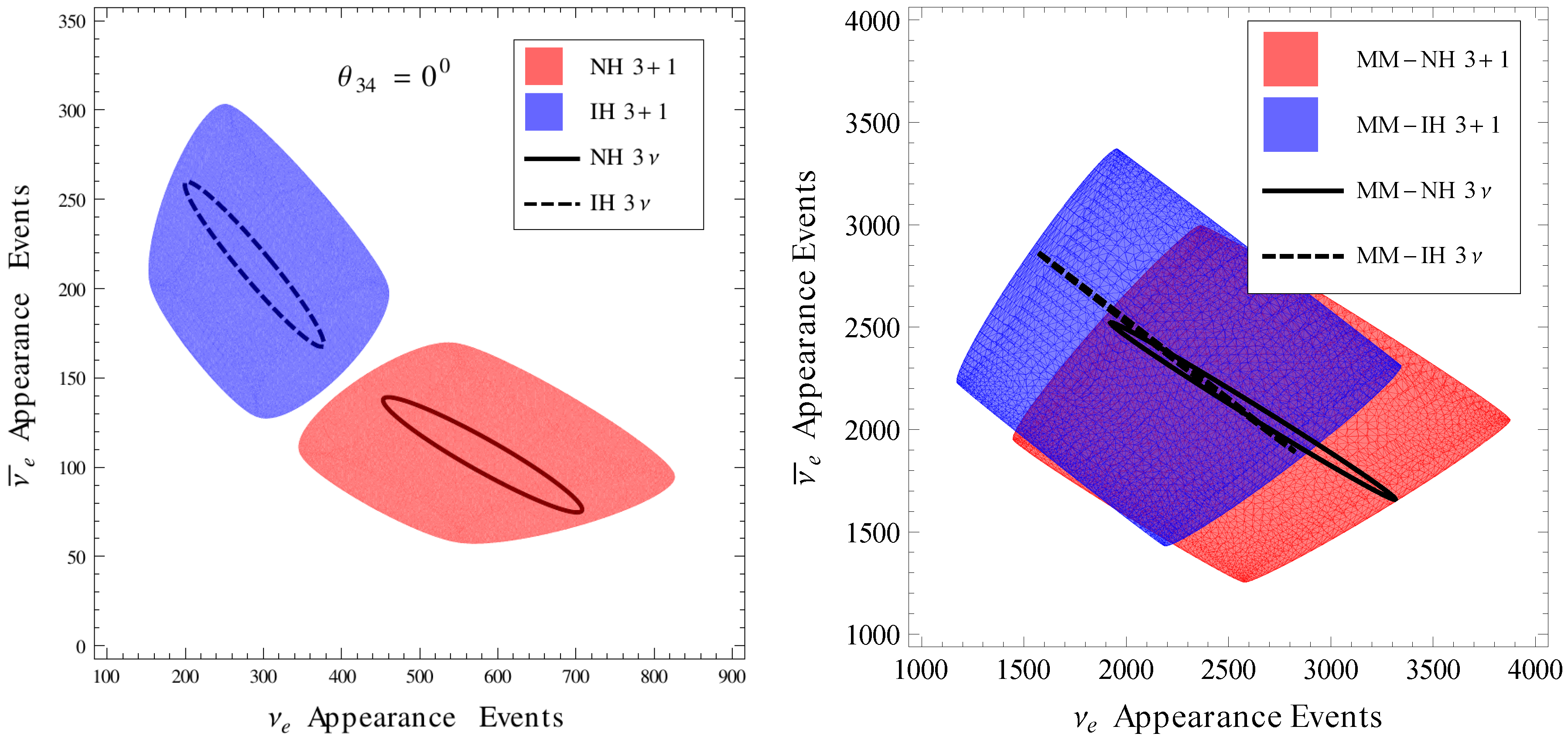
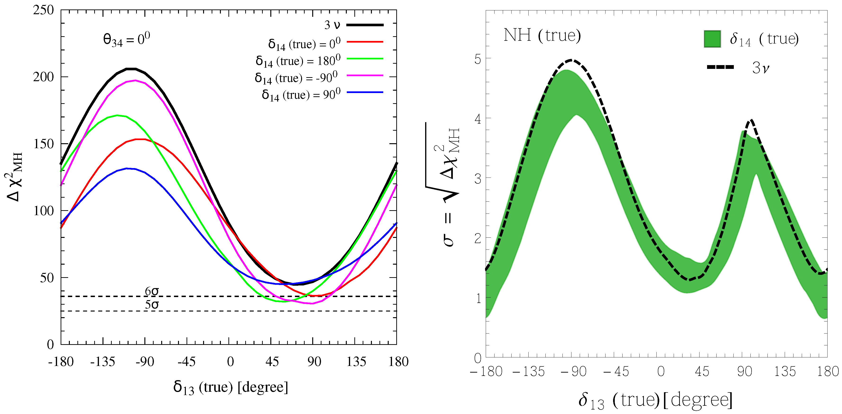
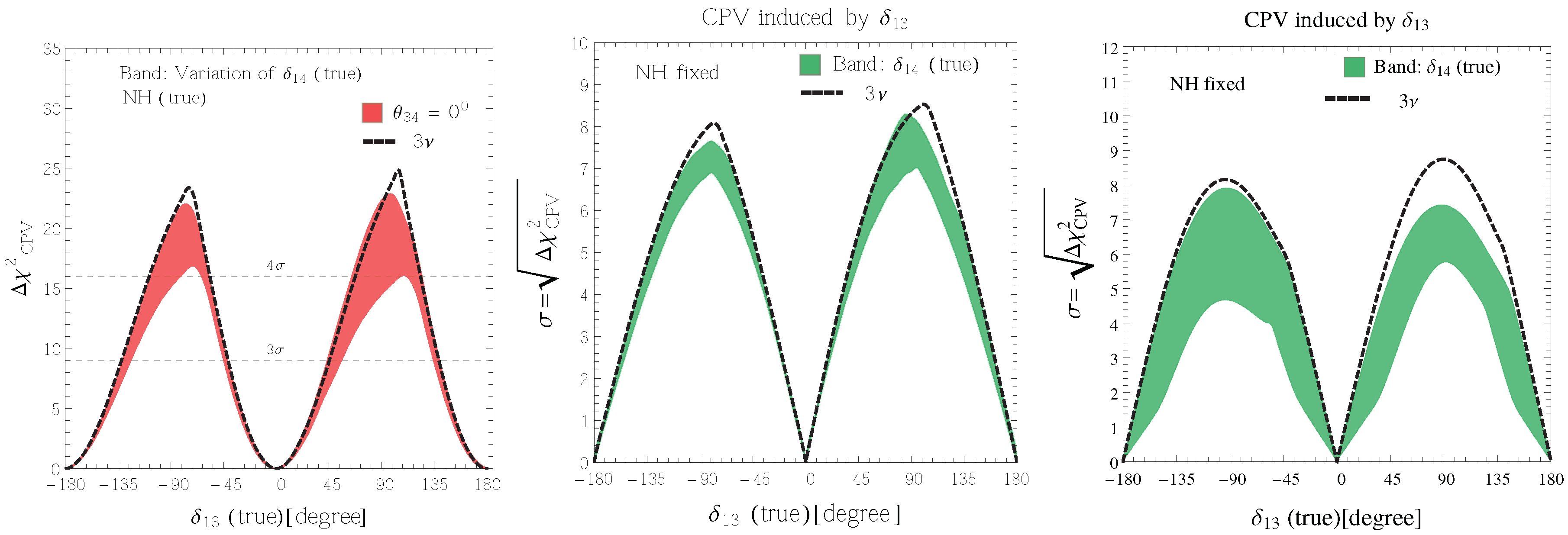
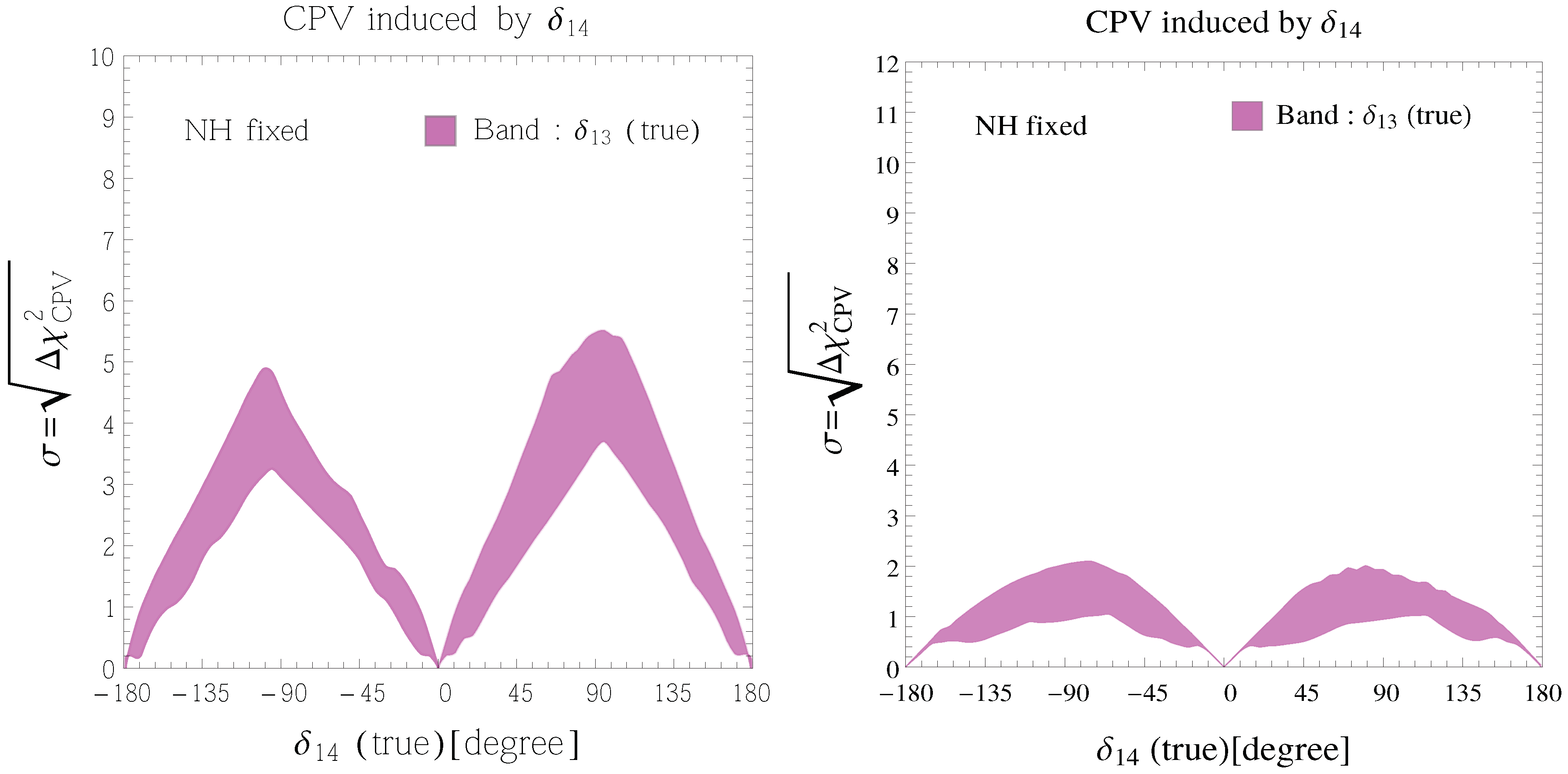
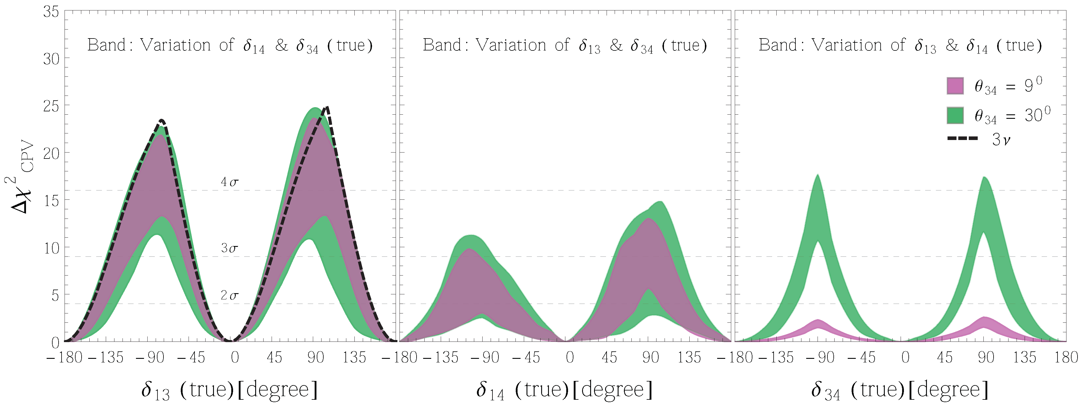
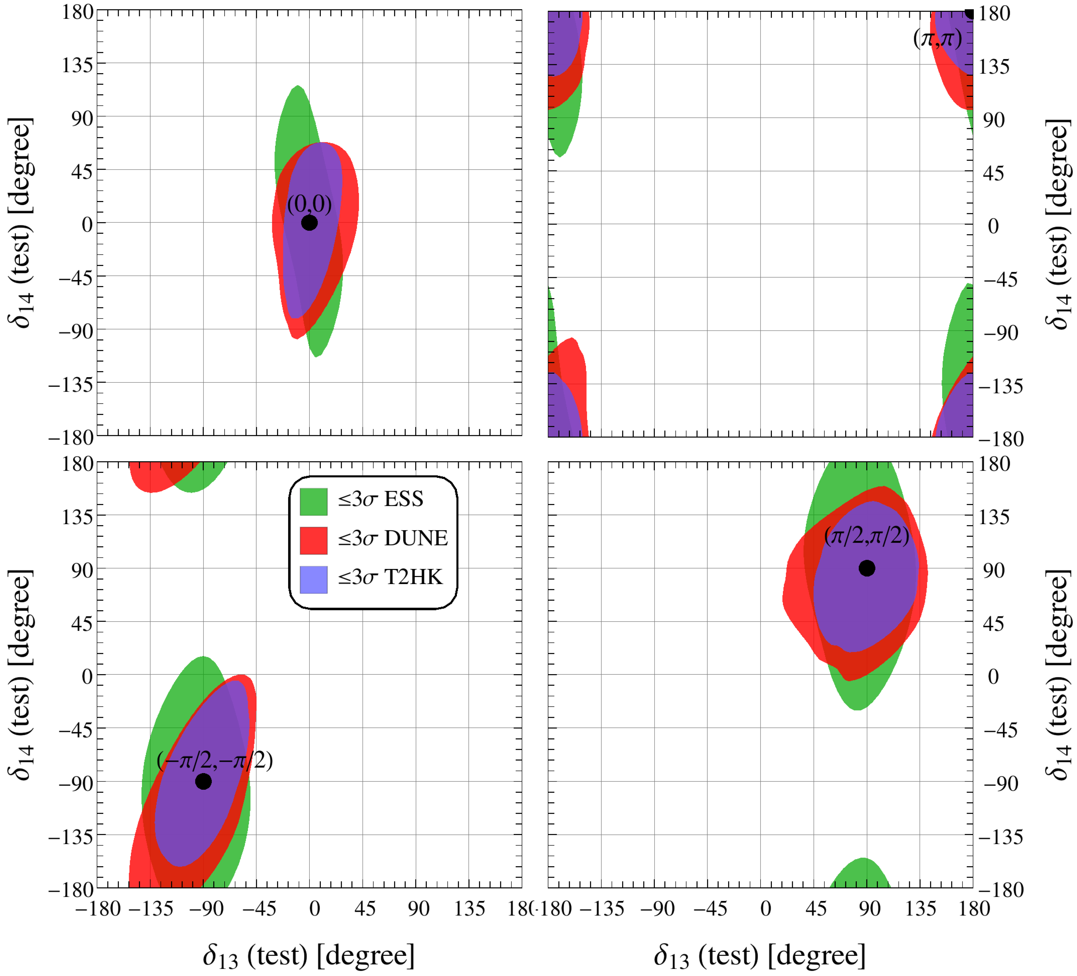
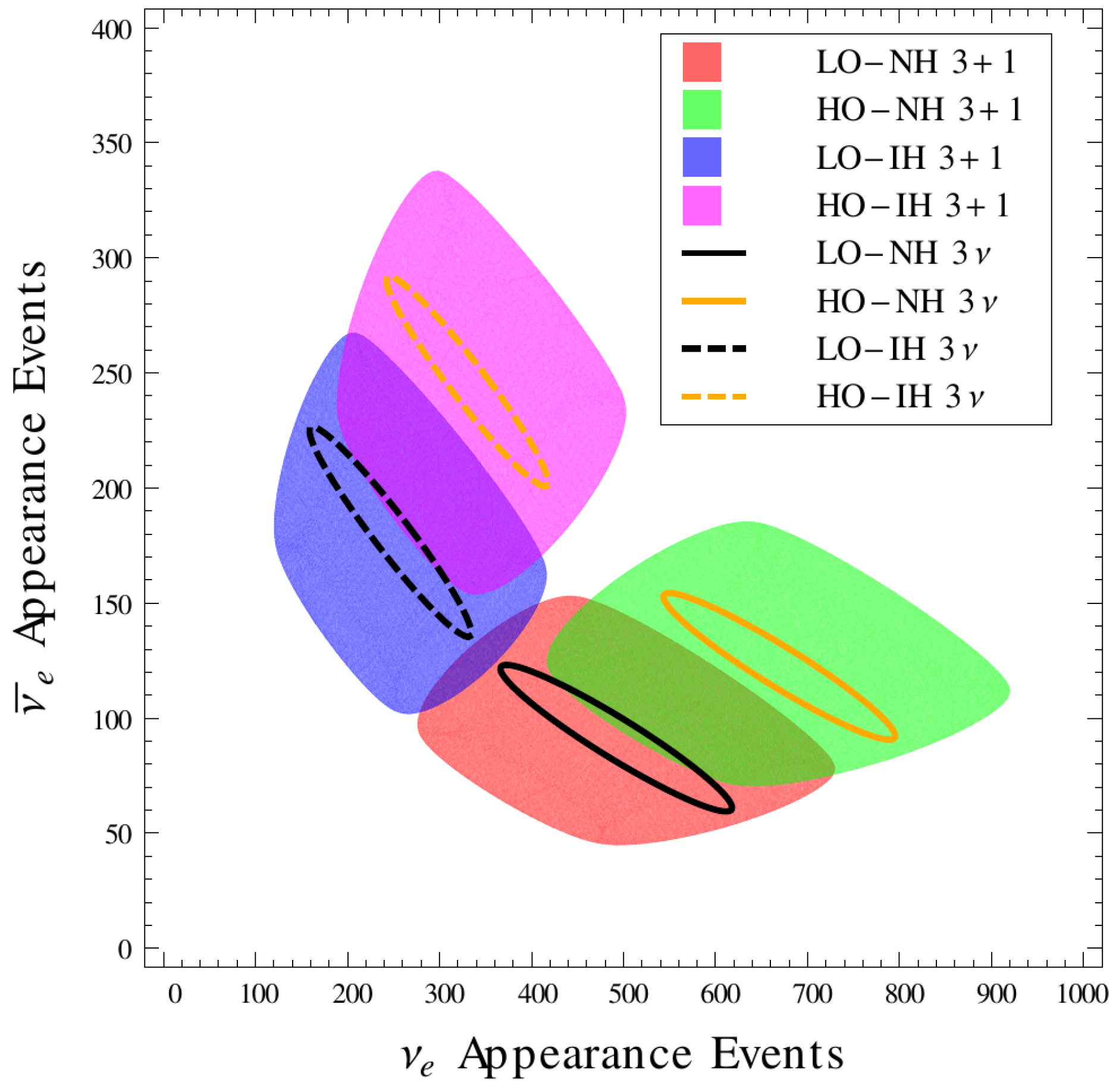
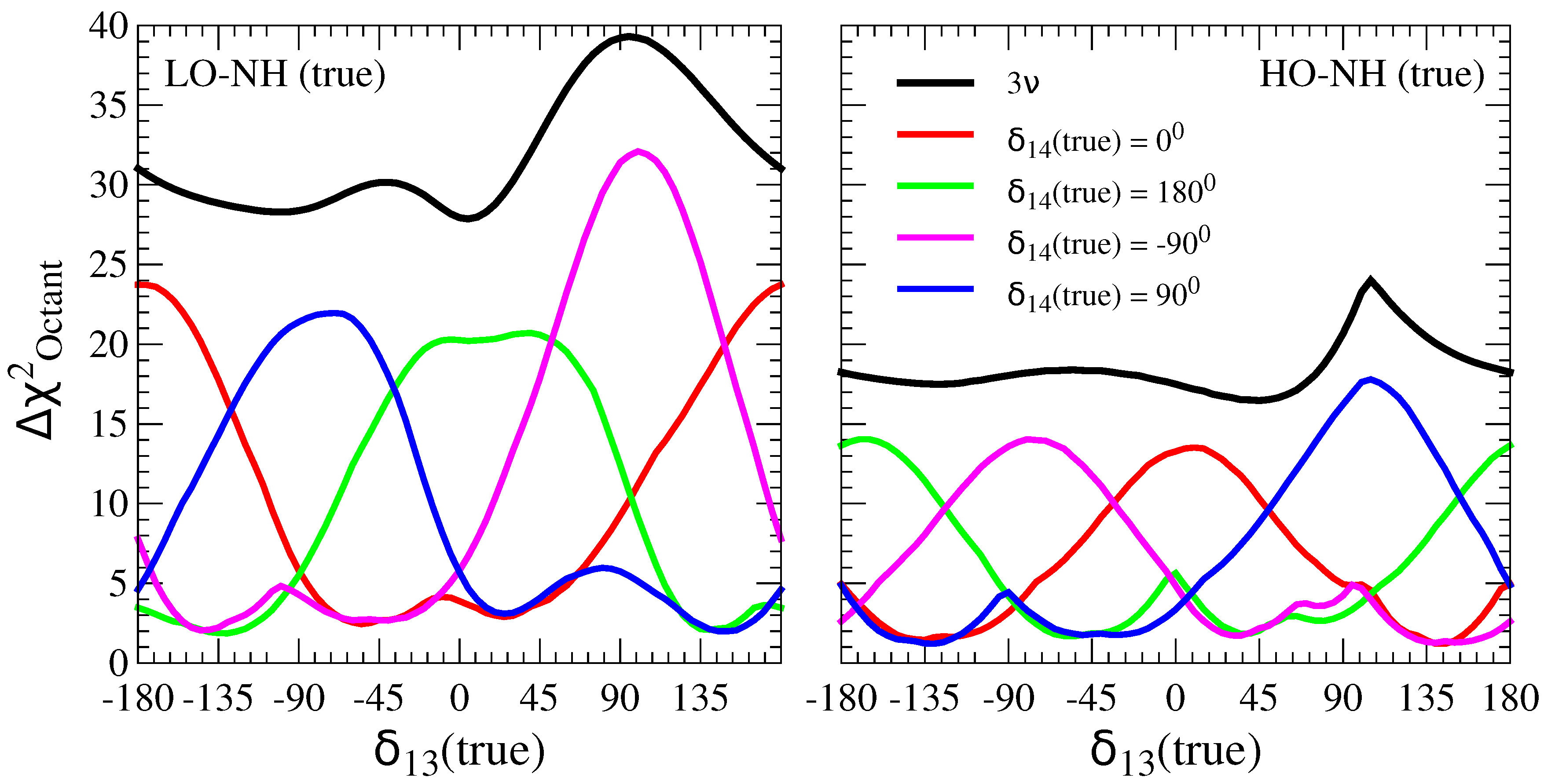
Table 1.
Parameter values and ranges used in the simulations. The second column displays the true values of the oscillation parameters used to simulate the true dataset. The third column displays the range over which and the CP-phases , , and are varied while minimizing the .
Table 1.
Parameter values and ranges used in the simulations. The second column displays the true values of the oscillation parameters used to simulate the true dataset. The third column displays the range over which and the CP-phases , , and are varied while minimizing the .
| Parameter | True Value | Marginalization Range |
|---|---|---|
| 0.304 | Not marginalized | |
| Not marginalized | ||
| 0.50 | [0.34, 0.68] | |
| 0.025 | Not marginalized | |
| 0.025 | Not marginalized | |
| 0, 0.025, 0.25 | Not marginalized | |
| [–180,180] | [–180,180] | |
| [–180,180] | [–180,180] | |
| [–180,180] | [–180,180] | |
| 7.50 | Not marginalized | |
| (NH) | 2.475 | Not marginalized |
| (IH) | –2.4 | Not marginalized |
| 1.0 | Not marginalized |
© 2020 by the author. Licensee MDPI, Basel, Switzerland. This article is an open access article distributed under the terms and conditions of the Creative Commons Attribution (CC BY) license (http://creativecommons.org/licenses/by/4.0/).
Share and Cite
MDPI and ACS Style
Palazzo, A. Exploring Light Sterile Neutrinos at Long Baseline Experiments: A Review. Universe 2020, 6, 41. https://doi.org/10.3390/universe6030041
AMA Style
Palazzo A. Exploring Light Sterile Neutrinos at Long Baseline Experiments: A Review. Universe. 2020; 6(3):41. https://doi.org/10.3390/universe6030041
Chicago/Turabian StylePalazzo, Antonio. 2020. "Exploring Light Sterile Neutrinos at Long Baseline Experiments: A Review" Universe 6, no. 3: 41. https://doi.org/10.3390/universe6030041
Note that from the first issue of 2016, this journal uses article numbers instead of page numbers. See further details here.