Bifurcation Analysis and Periodic Solutions of the HD 191408 System with Triaxial and Radiative Perturbations

Abstract

The nonlinear orbital dynamics of a class of the perturbed restricted three-body problem is studied. The two primaries considered here refer to the binary system HD 191408. The third particle moves under the gravity of the binary system, whose triaxial rate and radiation factor are also considered. Based on the dynamic governing equation of the third particle in the binary HD 191408 system, the motion state manifold is given. By plotting bifurcation diagrams of the system, the effects of various perturbation factors on the dynamic behavior of the third particle are discussed in detail. In addition, the relationship between the geometric configuration and the Jacobian constant is discussed by analyzing the zero-velocity surface and zero-velocity curve of the system. Then, using the Poincaré–Lindsted method and numerical simulation, the second- and third-order periodic orbits of the third particle around the collinear libration point in two- and three-dimensional spaces are analytically and numerically presented. This paper complements the results by Singh et al. [Singh et al., AMC, 2018]. It contains not only higher-order analytical periodic solutions in the vicinity of the collinear equilibrium points but also conducts extensive numerical research on the bifurcation of the binary system.

1. Introduction

As we know, approximately two-thirds of the stars are part of the multistellar system in our galaxy. Due to their diversity and the unpredictable characteristics of planets in our solar system, exploring the planets in the multistellar system is of great interest for many scientists. The planets in a multiplanetary system and celestial bodies constitute N-body problems.

Among the N-body problems, the three-body problem has been a hot research field because of its obvious practical value, and the most widely used model is the classical restricted three-body problem (RTBP). There are two important solutions in RTBP: Equilibrium points and periodic solutions. Several analytical and numerical methods for searching periodic solutions of restricted three-body problems can be found in the review article Musielak and Quarles [1]. Regarding the existence of periodic solutions of a circular RTBP, Gao and Zhang [2] gave a rigorous proof and found that the periodic solutions were mainly affected by factors such as the initial values and the masses of the two primaries.

When the restricted three-body problem is perturbed by some other factors (such as light pressure, oblate spheroidal primaries, radiation, and albedo, etc.), it will become the restricted three-body problem, which is closer to the natural system. Singh and his collaborators have done a lot of excellent research in this field. For example, Singh et al. [3,4] studied the existence of equilibrium points and the periodic orbits around the triangular equilibrium points of the perturbed RTBP, where the larger primary and smaller primary are considered triaxial and oblate spheroidal bodies, respectively. Moreover, Tsirogiannis et al. [5] and Singh et al. [6] considered a modification of the RTBP with radiation and oblateness and studied the periodic motions around the collinear equilibrium points. Furthermore, semi-analytical solutions around these points for both planar and spatial cases were obtained using the Lindstedt–Poincaré method by Singh et al. [6]. Kalantonis et al. [7] considered the asymptotic motion to collinear equilibrium points of the RTBP with the oblateness and they computed an asymptotic orbit by using a fourth-order local analysis, numerical integration, and standard differential corrections.

For the case of a planar circular RTBP, where the first primary is an oblate spheroid, and the oblateness coefficients affect the character of the orbits, Zotos [8] reported three types of orbits: Bounded, escaping, and collisional orbits. When the primaries are triaxial rigid bodies, Elshaboury et al. [9] investigated the basic dynamical characteristics of the RTBP and obtained the equilibrium points as well as some simple symmetric periodic orbits. For the RTBP with radiation and triaxiality, Jain et al. [10] analyzed the effects of these perturbations on periodic orbits under different energy constants. Furthermore, Idridi and Ullah [11] discussed the effects of the radiation and albedo on the existence of the noncollinear libration points in the elliptic RTBP, in which the oblateness of the second primary was considered.

In the past few decades, researchers have observed multiplanetary systems using space telescopes, observational data, and statistics tools (see Chen [12] for details). The binary system consisting of two stars moving around their common barycenter is particularly worth our attention. The periodic orbits are important keys to understand the motion of the third particle in the binary system. When two asteroids were approximated as triaxial ellipsoids, Hou et al. [13] studied the forced periodic orbits around the triangular libration points in a binary asteroid system influenced by the solar radiation pressure. Recently, a numerical method was proposed to search for three-dimensional periodic orbits by Shi et al. [14]. After applying this method to binary asteroid 1999 KW4, they found five kinds of periodic orbits of the binary system. By quantifying the detected set of planet masses and orbits, Howard and Fulton [15] efficiently made planet discovery and characterization. Berardo et al. [16] presented new observations of HIP 41378, and its possible orbital periods were obtained through observation. Singh et al. [17] studied the collinear equilibrium points and periodic motion around them in the RTBP for the binary HD 191408 system, where the two primaries are triaxial rigid bodies and emit radiation. Moreover, the effects of different parameters on the collinear equilibrium points were discussed. Das et al. [18] investigated the field of the radiating binary stellar system in the circular RTBP. Singh et al. [19] found three-dimensional periodic orbits around the collinear equilibrium points of the RTBP with oblate and radiating primaries. Singh and Umar [20] found that the positions of the third particle depended on the oblateness, radiation coefficients of the primaries, and the eccentricity of their orbits in the elliptic RTBP. They provided the numerical application of this problem in the stellar-oblate binary system.

HD 191408 is a high-velocity star that belongs to the southern hemisphere main-sequence stars with debris disks, and García and Gómez [21] studied their optical aperture polarimetry. The study of high-resolution, high-signal-to-noise spectra of field stars of different metallicities becomes an effective technique to tackle various problems related to the chemical evolution of the galaxy, and Abia et al. [22] provided the atmospheric parameters, elemental abundance ratio, and signal-to-noise ratios for some stars, including the parameters of HD 191408. Karaali et al. [23] investigated the metallicity calibration of several dwarfs and metal-poor stars at different distances from the galactic plane, which contribute to the implications for the galactic formation and evolution. In addition, Perrin [24] analyzed the chemical composition for twelve K dwarfs, whose masses were estimated. However, few researchers have studied the periodic solutions of this system.

Bifurcation refers to the motion of a system with suddenly changing parameters, e.g., the equilibrium state or the number and stability of the periodic motion, when the parameters change and become a certain value. Yumagulov et al. [25] studied the bifurcation in the planar elliptical RTBP, where the parameters of the system around the triangular equilibrium points were discussed. Perdomo [26] observed the reduced periodic solutions of the spatial isosceles three-body problem, which contained a bifurcation point and provided an explanation for the existence of this point. Maciejewski and Rybicki [27] studied global bifurcation from the equilibrium points of the nonstationary periodic solutions in the RTBP. There are also some other excellent related literatures [28,29,30,31], mainly including the reports of a binary system with short-orbital-period, the spatial periodic orbits in various resonances, and the periodic motions near a high mass ratio binary star system.

In this paper, we inherit the model of the perturbed restricted three-body problem of Singh et al. [17] and Jain et al. [10] and continue to study the binary HD 191408 system. In Section 2, the dynamical equations that involve the parameters of the third particle in the binary system are obtained. In Section 3, the bifurcation diagrams of the system’s state variables in terms of different parameters are illustrated and explained. In Section 4, the equilibrium points of the system are introduced by discussing the geometric configurations. In Section 5, the 2- and 3-dimensional periodic orbits around the collinear equilibrium points are computed using the Lindstedt–Poincaré method. Section 6 summarizes the study.

2. Dynamical Equations

For the sake of convenience, we first introduce the normal rotating dimensionless coordinate system $oxyz$, of which the origin is located in the centroid of two primary bodies with masses $m_1=1-\mu$ and $m_2=\mu$, where $\mu =m_2/\left(m_1+m_2\right)\in \left(0, 1\right)$. Assuming that the coordinate of the third particle is $\left(x, y, z\right)$, the two primaries are located at $\left(\mu , 0, 0\right)$ and $\left(\mu -1, 0, 0\right)$, respectively. According to Singh et al. [17] and Jain et al. [10], the equations of motion of the third particle are

$$\begin{array}{l}\ddot{x}-2\alpha n\dot{y}={\Omega }_x,\\ \ddot{y}+2\alpha n\dot{x}={\Omega }_y,\\ \ddot{z}={\Omega }_z,\end{array}$$

(1)

where α represents the modification of perturbation on the Coriolis force and the potential function $\mathsf{\Omega }\left(x,y,z\right)$ admits the following form

$$\begin{array}{l}\Omega \left(x,y,z\right)=\frac{n^2\beta }{2}(x^2+y^2)+\frac{(1-\mu )q_1}{r_1}+\frac{\mu q_2}{r_2}+\frac{(1-\mu )(2s_1-s_2)q_1}{2r_1{}^3}+\frac{\mu (2s_3-s_4)q_2}{2r_2{}^3}\\ \hspace{1em}\hspace{1em}-\frac{3(1-\mu )(s_1-s_2)y^2{q}_1}{2r_1{}^5}-\frac{3\mu (s_3-s_4)y^2{q}_2}{2r_2{}^5}-\frac{3(1-\mu )s_1{z}^2{q}_1}{2r_1{}^5}-\frac{3\mu s_3{z}^2{q}_2}{2r_2{}^5},\end{array}$$

(2)

$\beta$ denotes the modification of perturbation on the centrifugal force and $q_1$ and $q_2$ are the radiation factors of the primaries. In addition, $r_1=\sqrt{{(x-\mu )}^2+y^2+z^2}$ and $r_2=\sqrt{{(x+1-\mu )}^2+y^2+z^2}$ denote the distances between the third particle and the first and second primaries, respectively. On account of the triaxiality of the primaries, the mean perturbed motion $n$ is defined by

$$n=\sqrt{1+\frac{3}{2}\left[\left(2s_1-s_2\right)+\left(2s_3-s_4\right)\right]},$$

(3)

$$s_1=\frac{(a_1{}^2-a_3{}^2)}{5R^2}, s_2=\frac{(a_2{}^2-a_3{}^2)}{5R^2}, s_3=\frac{(a_1{}^{\prime 2}-a_3{}^{\prime 2})}{5R^2}, s_4=\frac{(a_2{}^{\prime 2}-a_3{}^{\prime 2})}{5R^2},$$

where $a_i\left(i=1, 2, 3\right)$ is the semi-axis of the first primary, ${a_i}^{\prime }\left(i=1, 2, 3\right)$ is the semi-axis of the second primary, and $R$ is the dimensional distance between the two primaries. The physical parameters of the binary HD 191408 system are shown in

Table 1. Physical parameters of the binary HD 191408 system [17].

Parameters	$\mu$	$s_1$	$s_2$	$s_3$	$s_4$	$q_1$	$q_2$	$\alpha$	$\beta$
Values	0.1881	0.008	0.004	0.002	0.001	0.407761	0.991476	1.0003	1.0002

.

The first Jacobi-type function of the system (1) is

$$2\Omega \left(x,y,z\right)-\left({\dot{x}}^2+{\dot{y}}^2+{\dot{z}}^2\right)=C ,$$

(4)

where $V^2={\dot{x}}^2+{\dot{y}}^2+{\dot{z}}^2$ is the motion velocity of the third particle and C is the Jacobi constant.

3. Analysis of the Bifurcation and Chaos

In this section, the bifurcation diagrams of the state variables in terms of different parameters in the binary HD 191408 system are illustrated, and the effects of each parameter on the system are analyzed.

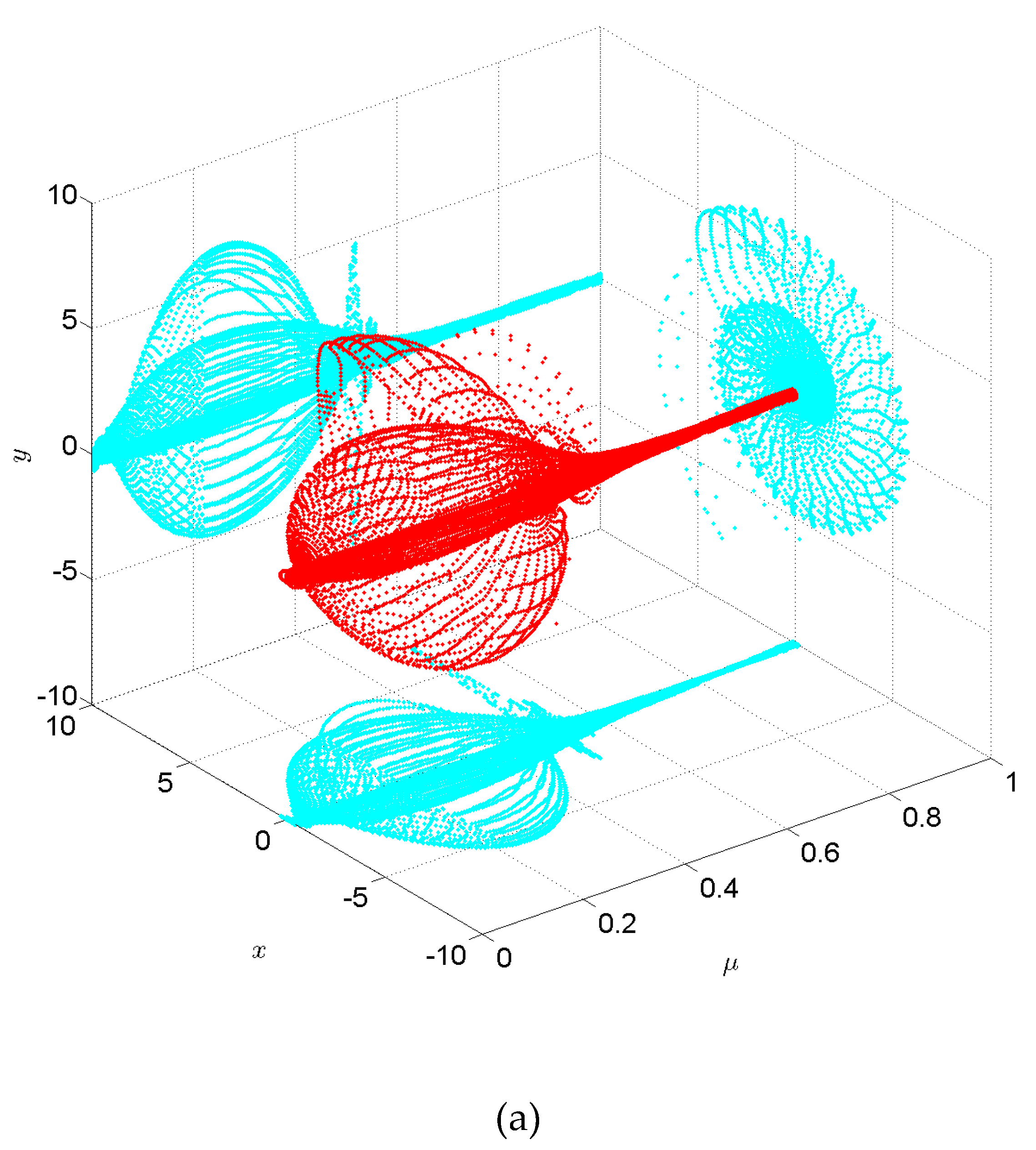
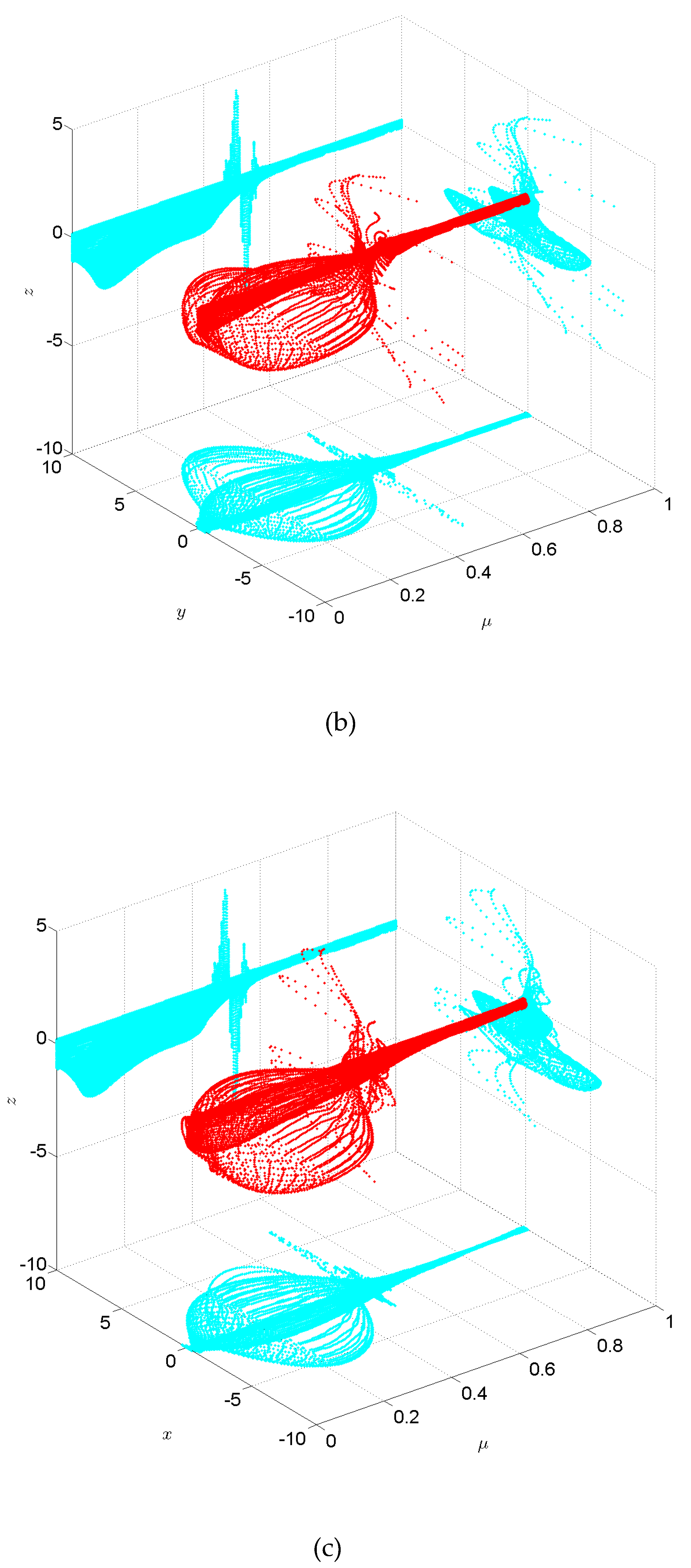
For the given values of Table 1, we selected the iterative initial value $x_0=\left(-0.08,0.001,0.2,0,-1.6,0\right)$ and limit parameter $\mu$ in the interval $\left(0,1\right)$. By applying the ode45 numerical integration algorithm [32], we obtain the results in Figure 1; namely, the bifurcation diagrams of three state variables, frames of $\mu xy$, $\mu yz$, and $\mu xz$, in terms of mass parameter $\mu$ in the binary HD 191408 system. Figure 1a shows the effect of $\mu$ in the $\mu xy$ frame; for a given value of $\mu$, the bifurcation diagram in the $\mu xy$ frame in terms of $\mu$ is obtained. Figure 1a also shows the bifurcation diagrams of variables $x$ and $y$ in terms of $\mu$, i.e., the projection from the three-dimensional diagram to the two-dimensional plane. The projections have similar structure, which is inevitable in qualitative analysis by comparing the projections. Similarly, the bifurcation diagrams in the $\mu yz$ and $\mu xz$ frames in terms of $\mu$ are shown in Figure 1b,c.

For each different initial value, system (1) will admit different bifurcation diagrams, but for a given initial value, we can analyze the influence of the change of perturbation parameters on the dynamic behavior of the third particle by displaying a set of bifurcation diagrams. For example, we can find clearly from Figure 1 that chaotic motion exists in the three directions of space for the third particle when the mass parameter $\mu \in \left(0, 0.5\right]$. Especially when $\mu =0.5$ or so, that is to say, when the masses of two primaries are approximately equal, the dynamic behavior of the third particle changes greatly. However, its dynamic behavior decreases significantly when $\mu \in \left(0.5, 1\right)$.

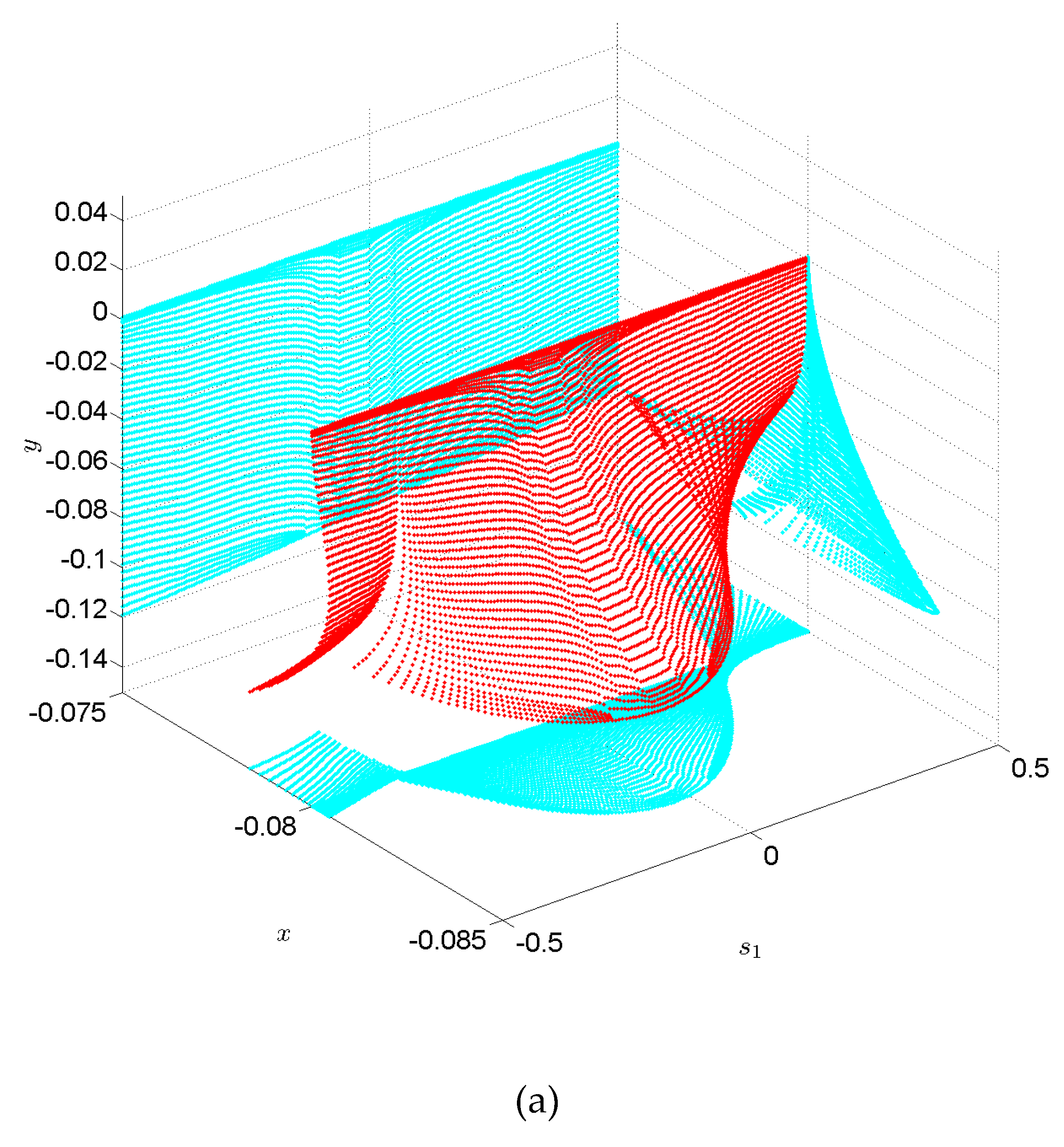
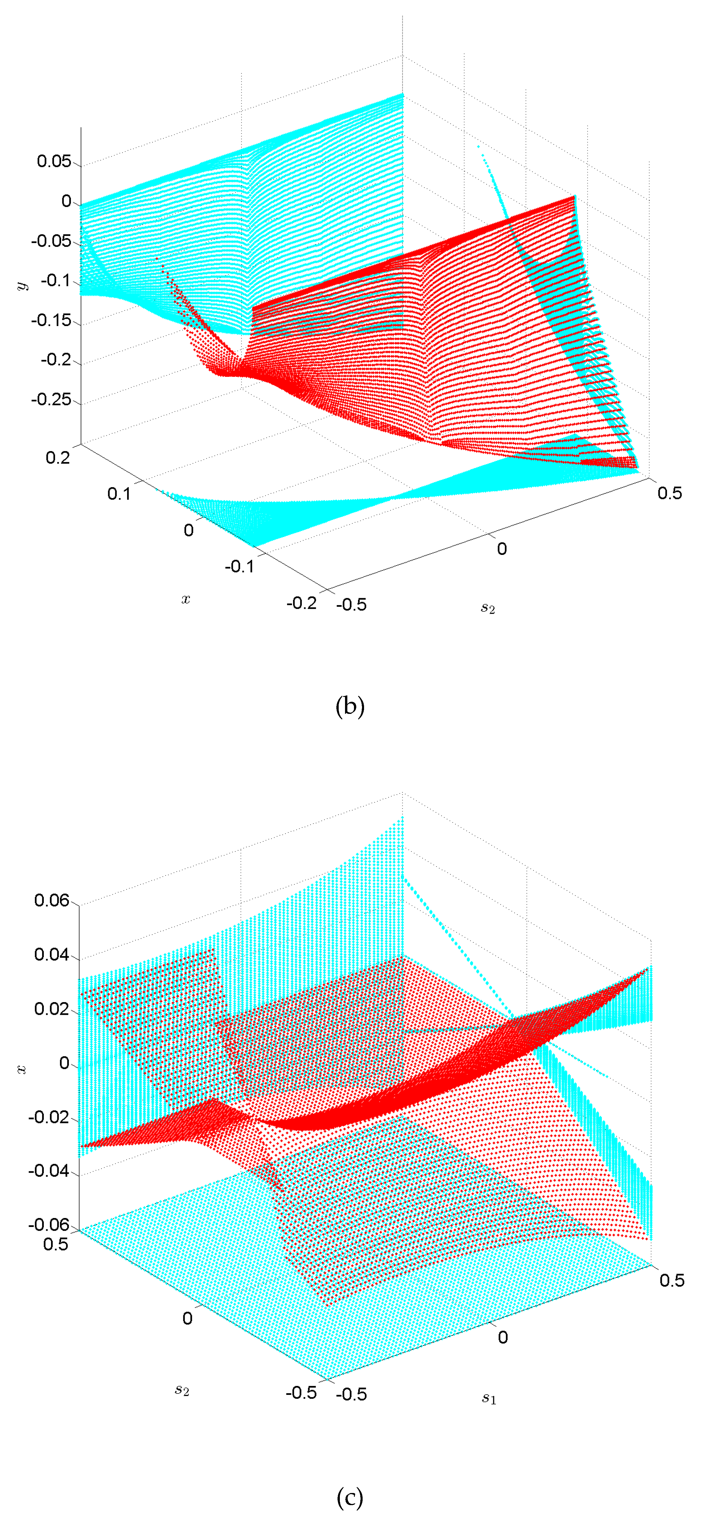
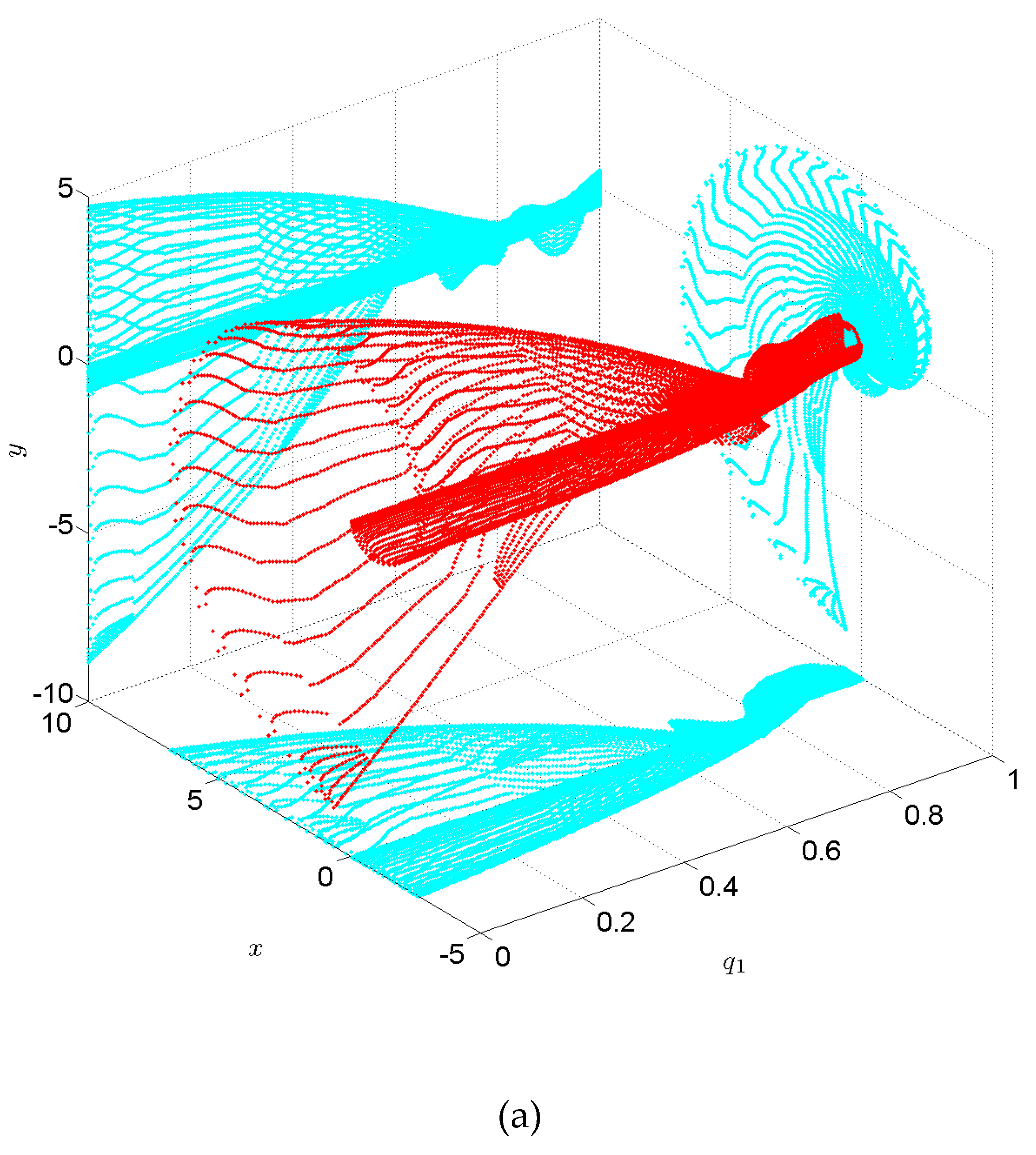
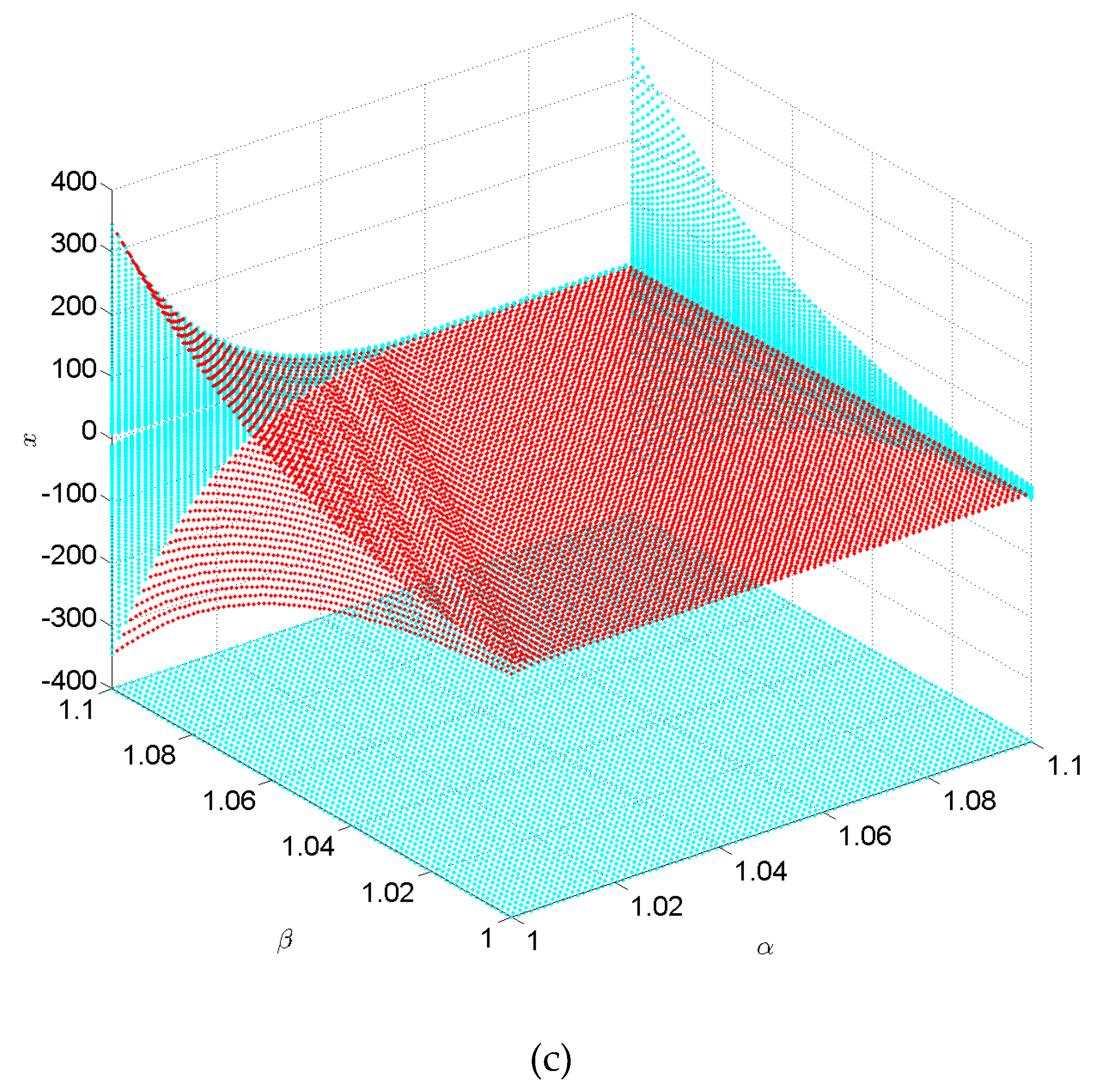
Similarly, we select $x_0$ and restrict the triaxial coefficient $s_i \left(i=1, 2, 3, 4\right)$ to the interval $\left[-0.5, 0.5\right]$. The bifurcation diagrams of the state variables with respect to the triaxial coefficient $s_i \left(i=1, 2, 3, 4\right)$ are shown in Figure 2 and Figure 3. Figure 2a shows that the triaxial coefficient $s_1$ of the first primary has little effect on the motion amplitude of the third particle in the $y$ direction, although it will cause the overall displacement of the third particle in this direction. It has a great influence on the movement of the third particle in the $x$ direction, especially when $s_1$ takes the threshold value around ±0.32, the movement of the third particle in the $x$ direction will be the opposite. Figure 2b shows that the triaxial coefficient $s_2$ of the first primary will cause the motion amplitude of the third particle to expand gradually in the $y$ direction, and when $s_2$ takes the threshold value of $-$0.07 in the $x$ direction, the movement of the third particle in this direction will also be in the opposite direction. Figure 2c shows that the combination of the triaxial coefficients $s_1$ and $s_2$ acts on the third particle in the $x$ direction. The result shows that the effect on the dynamic behavior of the third particle is greater when their values pass the threshold $s_1=-0.32$ and $s_2=-0.07$.

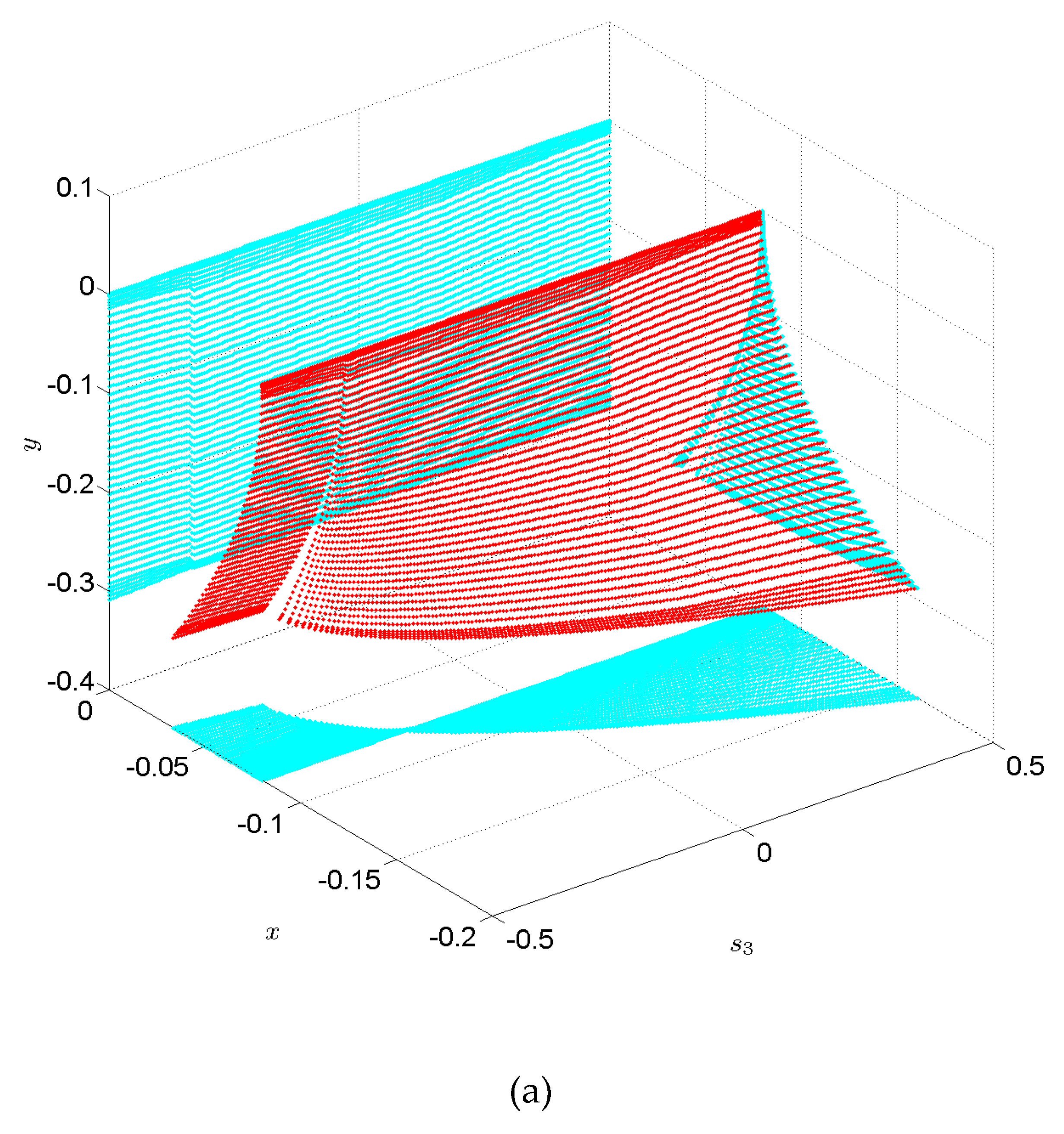
Figure 3 reflects the effect of the three semi-axes perturbations of the second primary on the dynamics of the third particle. Figure 3a shows that $s_3$ has little effect on the movement amplitude of the third particle in the $y$ direction, except that the third particle will have an overall shift in this direction. In the $x$ direction, when the value of $s_3$ passes the threshold value of −0.2, the movement of the third particle will change greatly. Figure 3b shows that the effect of $s_4$ on the movement of the third particle in $x$ and $y$ directions is extremely complex, and obvious chaos has appeared. Figure 3c shows that under the joint action of $s_3$ and $s_4$, with the increase of $s_3$ and the decrease of $s_4$, the dynamic behavior of the third particle in the $x$ direction tends to be stable.

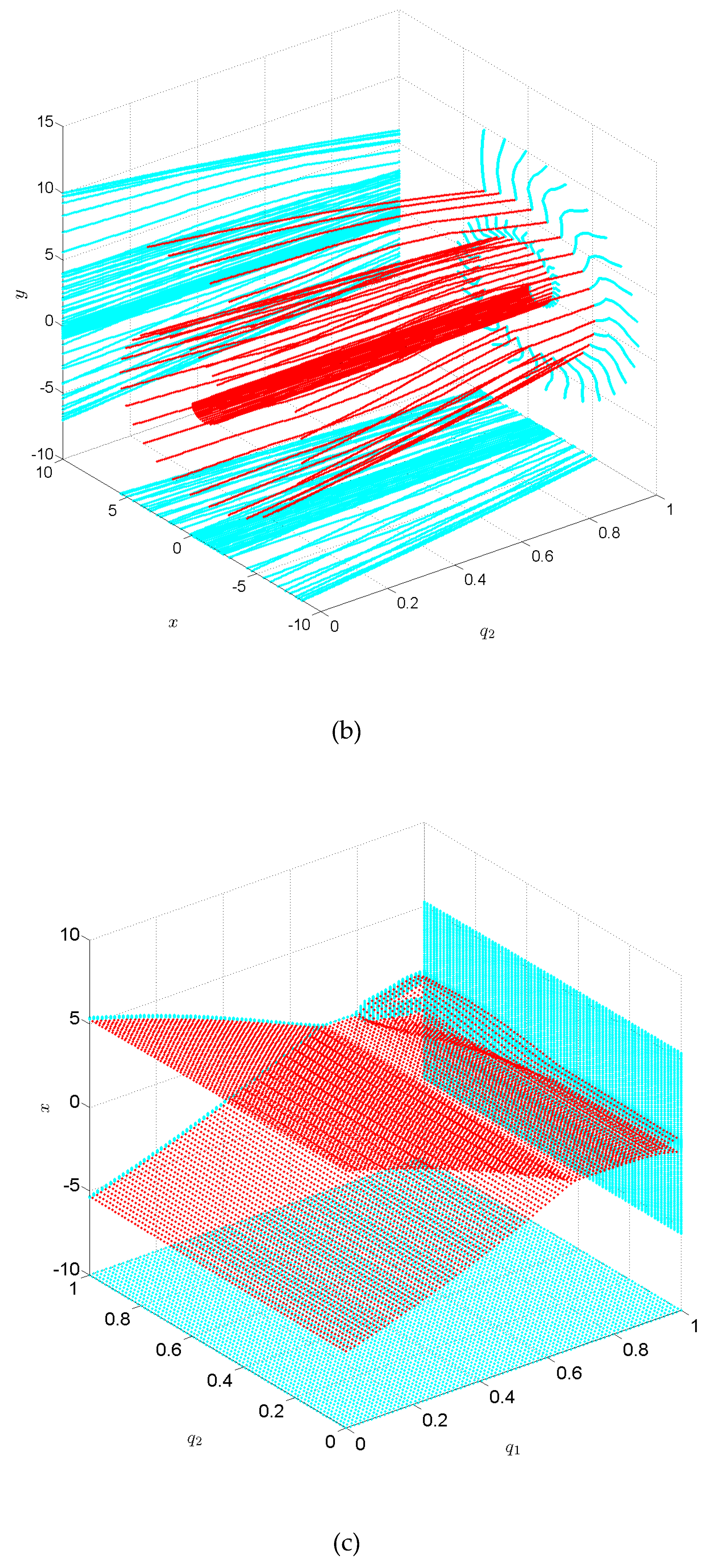
Next we select $x_0$ and restrict the radiation coefficient $q_i \left(i=1, 2\right)$ to the interval $\left[0, 1\right]$. Figure 4 reflects the influence of the radiation factors $q_i \left(i=1, 2\right)$ of the primaries on the dynamic behavior of the third particle. Figure 4a shows that the effect on the third particle in the $x$ and $y$ directions is the same basically, both of which are gradually reduced from large-scale movements as the radiation factor $q_1$ increases. It can be found from Figure 4b that the change of radiation factor $q_2$ has little effect on the dynamic behavior of the third particle, but under the combined effect of radiation factors $q_1$ and $q_2$ (see Figure 4c), the third particle exhibits periodic motion in the $x$ direction when $q_1\in \left[0.7, 0.8\right]$.

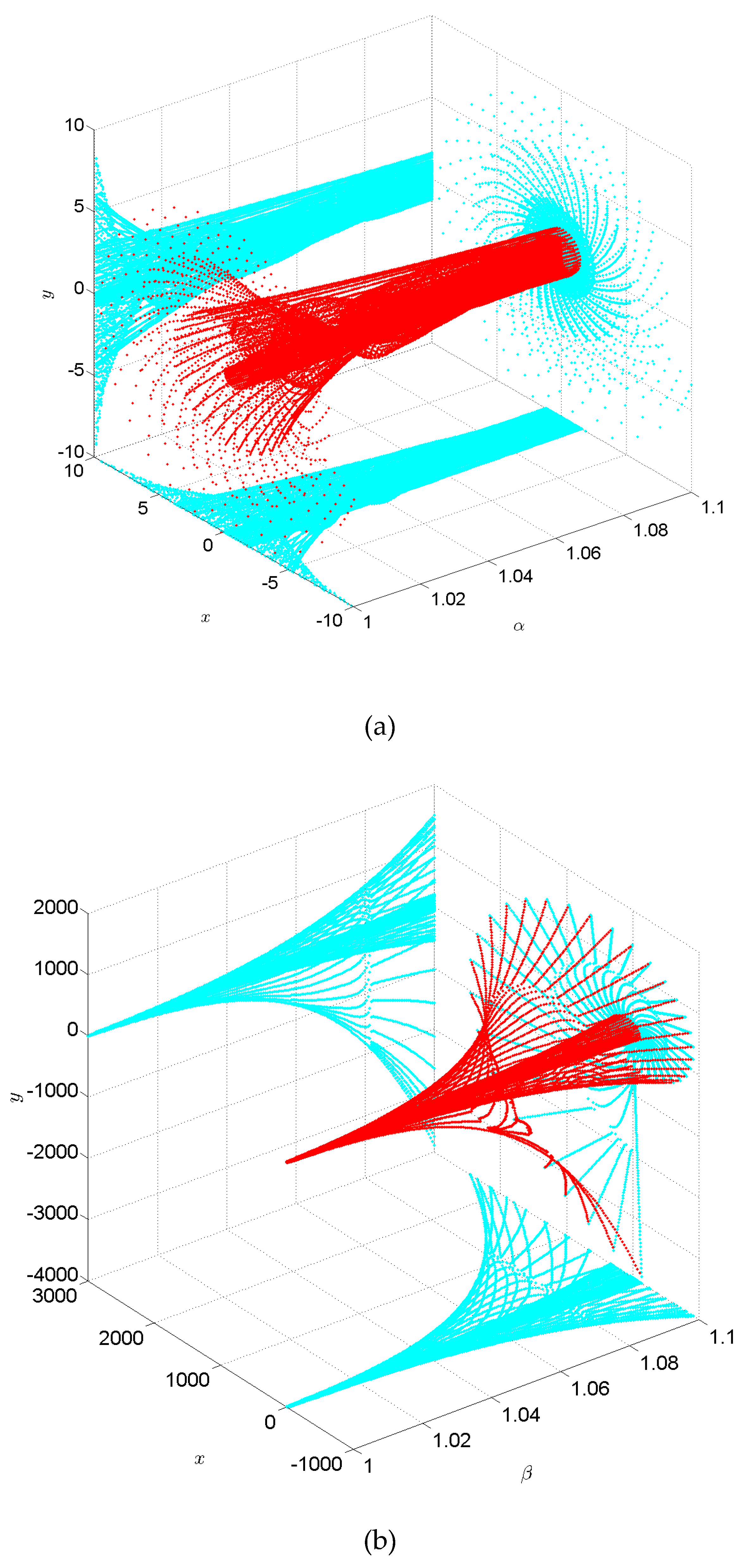
For the values of the Coriolis and centrifugal forces, which are restricted in the interval $\left[1, 1.1\right]$. The bifurcation diagram in Figure 5a shows that the modification in the Coriolis force $\alpha$ has a similar effect on the third particle in the $x$ and $y$ directions, both of which tend to a certain range gradually with the increase of $\alpha$ from large-scale motion. From Figure 5b, we find that the movement of the third particle in the $x$ and $y$ directions appears divergent as the modification in the centrifugal force $\beta$ increases; that is, the movement amplitude in both directions increases. However, the third particle shows periodic motion in the $x$ direction with the increase of $\alpha$ and $\beta$.

4. Equilibrium Points

For the Jacobi-type function (4) of the system, when the motion velocity of the third particle is zero, the three-dimensional space of the system with the change of Jacobi constant C is shown in Figure 6, Figure 7, Figure 8, Figure 9 and Figure 10. When C decreases from C = 3, five equilibrium points A, B, D, E, and F can be obtained. A smaller C value corresponds to the larger permissible regions of motion of the third particle. The specific analysis is as follows:

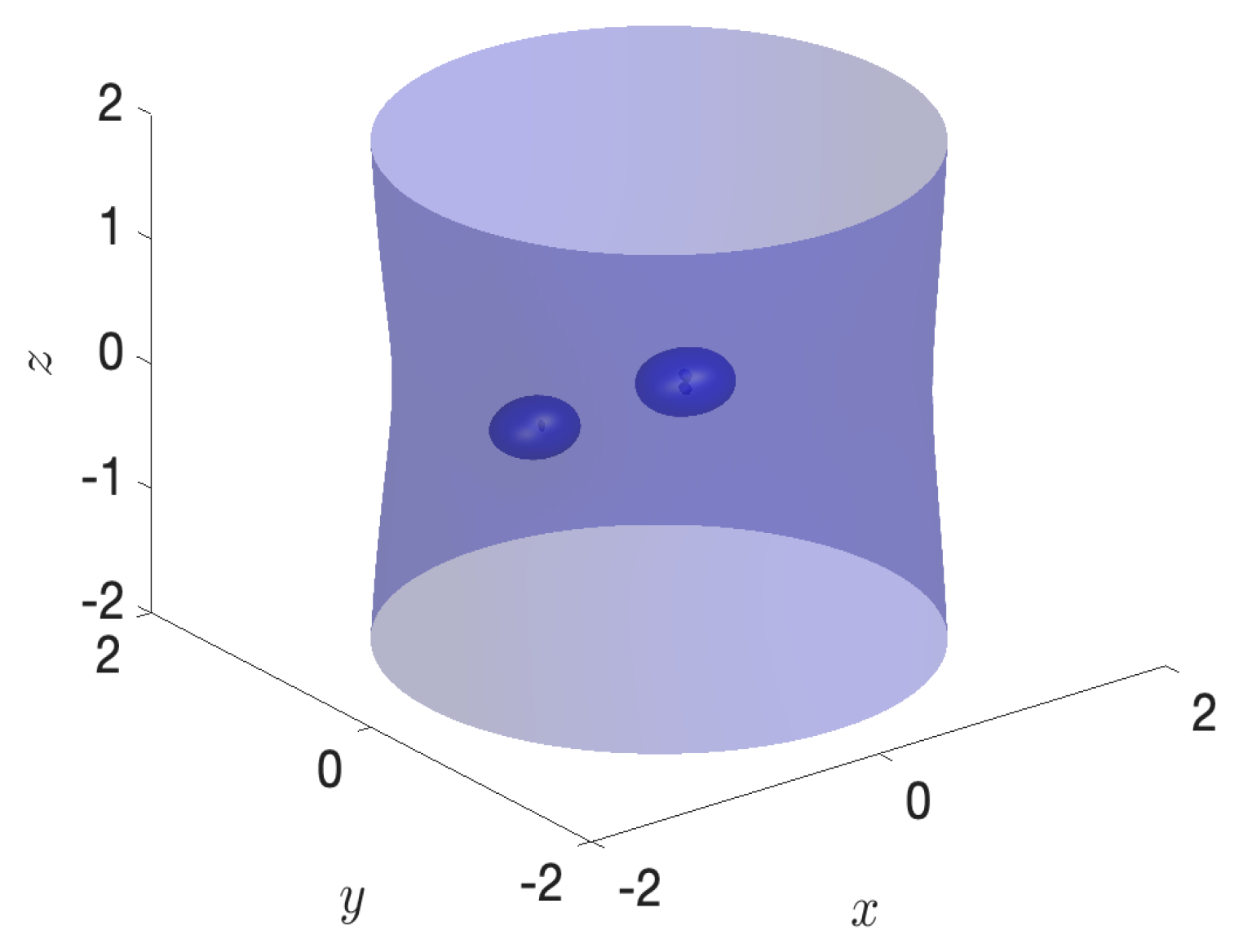
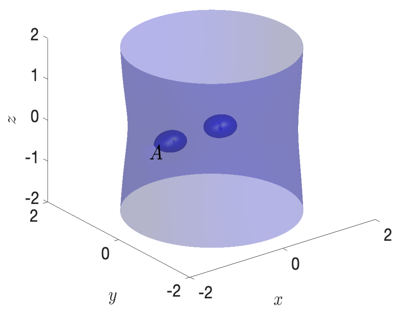
When C = 3, the zero-velocity surface of the third particle is shown in Figure 6. The third particle can only skim over two primaries under the action of gravity but cannot pass through the forbidden area around them. When C = 2.914, the forbidden area of one of the primaries and the outer forbidden one will intersect at point A (see Figure 7). The third particle can fly to the outer space through the channel A. In fact, this point A is the first equilibrium point.

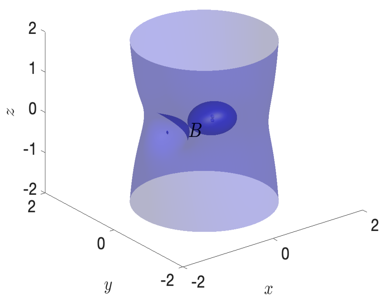
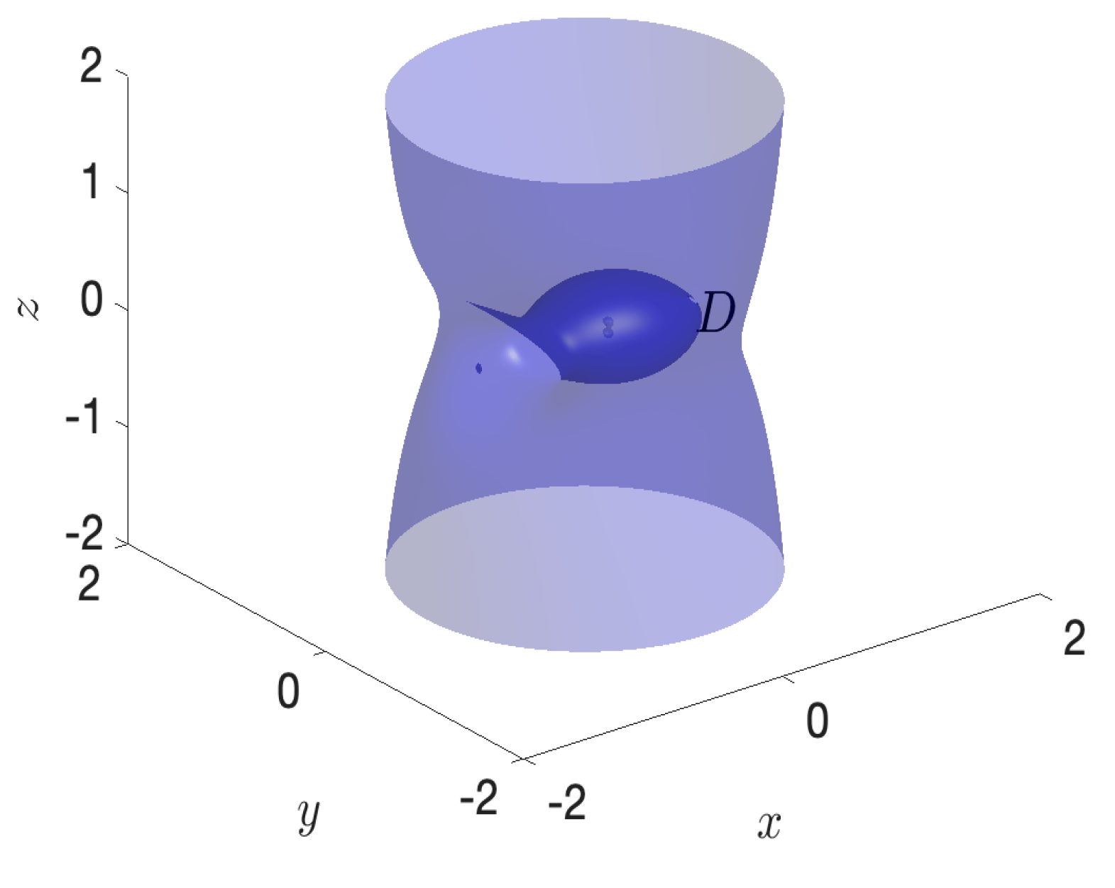
When C is 2.1943, as shown in Figure 8, the prohibited region of the third particle decreases. The “Channel B” appears, through which the third particle can fly from the permissible regions of one primary to another. Meanwhile, the second equilibrium point can be obtained. When C drops to 1.9777 (see Figure 9), “Channel D” appears, where the third particle can fly into another outer space. Thus, the third equilibrium point appears.

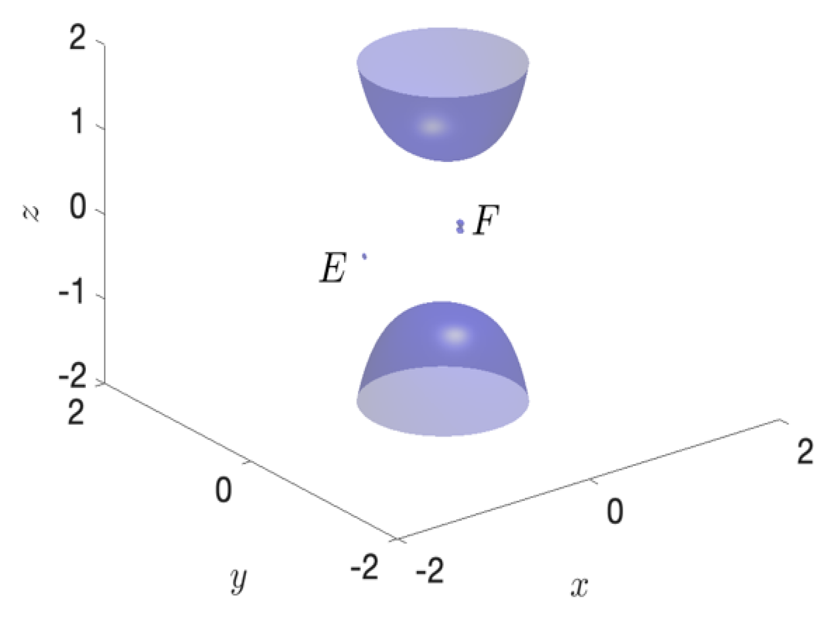
When C = 1 (see Figure 10), the last two equilibrium points E and F appear. With the decrease of C, the third particle can remove the primaries to fly into outer space.

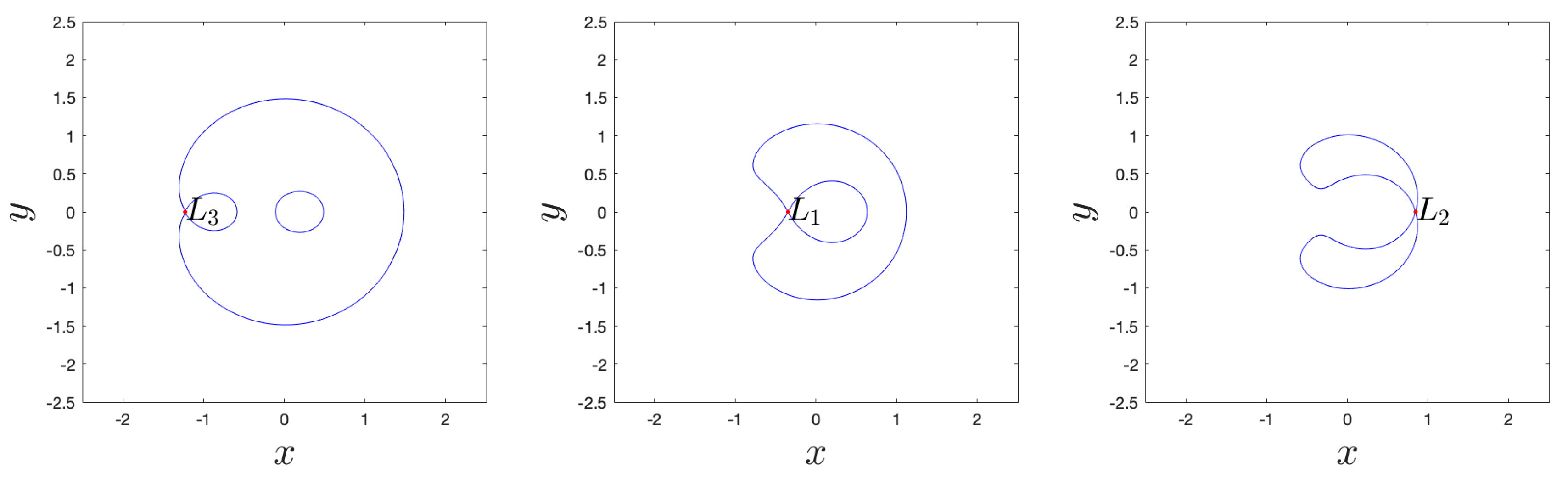
According to the discussion of zero velocity surface, when C takes 2.914, 2.1943, and 1.9777, the related zero velocity curves are shown in Figure 11. Therefore, three collinear equilibrium points are $L_1\left(-0.34630003, 0\right)$, $L_2\left(0.84584372, 0\right)$, and $L_3\left(-1,23037223, 0\right)$, respectively.

5. Periodic Orbits Around the Collinear Equilibrium Points

5.1. Expansion of The 2D Equations of Motion

In the plane, the motion equations of the third particle are (see [17])

$$\begin{array}{l}{\ddot{x}}_1-2\alpha n{\dot{x}}_2={\Omega }_{x_1},\\ {\ddot{x}}_2+2\alpha n{\dot{x}}_1={\Omega }_{x_2},\end{array}$$

(5)

where $x_1=x, x_2=y$ and the potential function in Equation (5) is

$$\begin{array}{l}\Omega =\frac{n^2\beta }{2}(x_1{}^2+x_2{}^2)+\frac{(1-\mu )q_1}{r_a}+\frac{\mu q_2}{r_b}+\frac{(1-\mu )(2s_1-s_2)q_1}{2r_a{}^3}+\frac{\mu (2s_3-s_4)q_2}{2r_b{}^3}\\ -\frac{3(1-\mu )(s_1-s_2)x_2{}^2{q}_1}{2r_a{}^5}-\frac{3\mu (s_3-s_4)x_2{}^2{q}_2}{2r_b{}^5}.\end{array}$$

(6)

Deriving the derivation with respect to $x_1$ and $x_2$ on the right side of Equation (6), we obtain

$$\begin{array}{l}{\Omega }_{x_1}=n^2\beta x_1-\frac{(1-\mu )q_1(x_1-\mu )}{r_a{}^3}-\frac{\mu q_2(x_1+1-\mu )}{r_b{}^3}-\frac{3(1-\mu )(2s_1-s_2)q_1(x_1-\mu )}{2r_a{}^5}\\ -\frac{3\mu (2s_3-s_4)q_2(x_1+1-\mu )}{2r_b{}^5}+\frac{15(1-\mu )(s_1-s_2)x_2{}^2{q}_1(x_1-\mu )}{2r_a{}^7}+\frac{15\mu (s_3-s_4)x_2{}^2{q}_2(x_1+1-\mu )}{2r_b{}^7},\\ {\Omega }_{x_2}=n^2\beta x_2-\frac{(1-\mu )q_1{x}_2}{r_a{}^3}-\frac{\mu q_2{x}_2}{r_b{}^3}-\frac{3(1-\mu )(4s_1-3s_2)q_1{x}_2}{2r_a{}^5}-\frac{3\mu (4s_3-3s_4)q_2{x}_2}{2r_b{}^5}\\ +\frac{15(1-\mu )(s_1-s_2)q_1{x}_2{}^3}{2r_a{}^7}+\frac{15\mu (s_3-s_4)q_2{x}_2{}^3}{2r_b{}^7},\end{array}$$

where $r_a=\sqrt{{\left(x_1-\mu \right)}^2+x_2{}^2}, r_b=\sqrt{{\left(x_1+1-\mu \right)}^2+x_2{}^2}$ are the distances between the third particle and the primaries. By substituting the transformation of $x_1=x_{L_i}+\xi$ and $x_2=\eta$ into Equation (5), we obtain the following equations of motion of the third particle

$$\begin{array}{l}\ddot{\xi }-2\alpha n\dot{\eta }={\Omega }_{\xi },\\ \ddot{\eta }+2\alpha n\dot{\xi }={\Omega }_{\eta }.\end{array}$$

(7)

Expand the right side of Equation (7) to the second order and get

$$\begin{array}{l}\ddot{\xi }-2\alpha n\dot{\eta }=K_1\xi +K_2{\xi }^2+K_3{\eta }^2,\\ \ddot{\eta }+2\alpha n\dot{\xi }=L_1\eta +L_2\xi \eta ,\end{array}$$

(8)

and to the third order, as follows

$$\begin{array}{l}\ddot{\xi }-2\alpha n\dot{\eta }=K_1\xi +K_2{\xi }^2+K_3{\eta }^2+K_4{\xi }^3+K_5\xi {\eta }^2,\\ \ddot{\eta }+2\alpha n\dot{\xi }=L_1\eta +L_2\xi \eta +L_3{\xi }^2\eta +L_4{\eta }^3,\end{array}$$

(9)

where the coefficients as shown in Appendix A.

5.2. Periodic Orbits in the Plane

Now, we examine the periodic solutions of system (5). Suppose that the periodic solutions of system (8) has the following form in the powers of orbital parameter $e \left(\left|e\right|\ll 1\right)$

$$\begin{array}{l}\xi ={\xi }_{1}e+{\xi }_2{e}^2,\\ \eta ={\eta }_{1}e+{\eta }_2{e}^2,\end{array}$$

(10)

By substituting Equation (10) into (8) and the series expansion of periodic solution with respect to $e$ is as follows

$$\begin{array}{l}\xi ={\xi }_0+\cos (\omega t)e+\left[{\varpi }_{21}+{\varpi }_{23}\cos (2\omega t)\right]e^2,\\ \eta =v_{12}\sin (\omega t)e+v_{24}\sin (2\omega t)e^2,\end{array}$$

(11)

where $\left({\xi }_0,0\right)$ denotes the position of the collinear equilibrium points in the previous section.

Similarly, we suppose that the periodic solutions of system (9) in powers of $e$ are

$$\begin{array}{l}\xi ={\xi }_{1}e+{\xi }_2{e}^2+{\xi }_3{e}^3,\\ \eta ={\eta }_{1}e+{\eta }_2{e}^2+{\eta }_3{e}^3, \end{array}$$

(12)

Thus, the periodic solution of system (5) into series expansions of $e$ up to the third-order terms is

$$\begin{array}{l}\xi ={\xi }_0+\cos (\omega t)e+\left[{\varpi }_{21}+{\varpi }_{23}\cos (2\omega t)\right]e^2+{\varpi }_{34}\cos (3\omega t)e^3,\\ \eta =v_{12}\sin (\omega t)e+v_{24}\sin (2\omega t)e^2+v_{36}\sin (3\omega t)e^3,\end{array}$$

(13)

where the coefficients are shown in Appendix B.

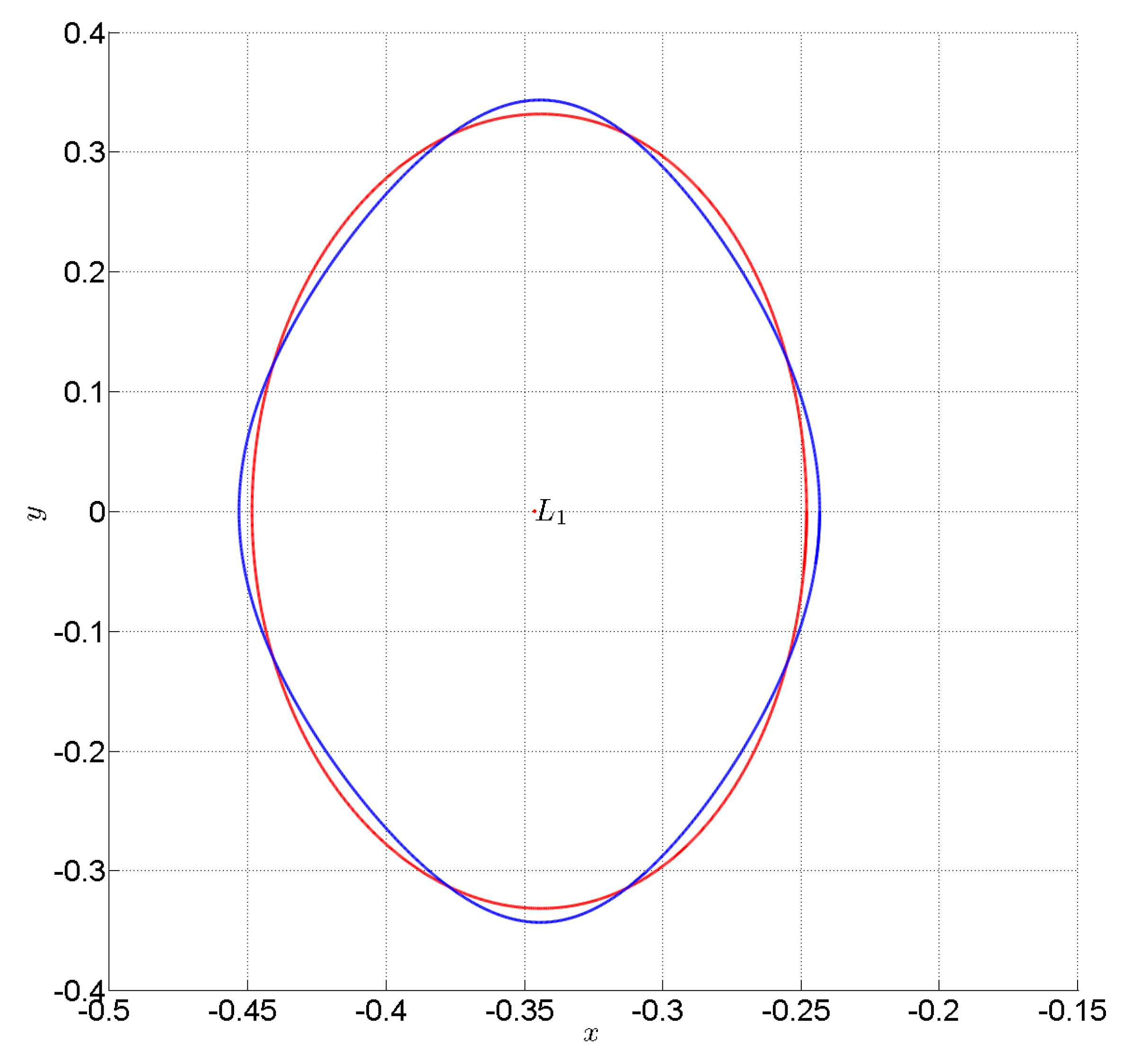
For the collinear equilibrium point $L_1\left(-0.34630003, 0\right)$ around which the periodic orbits are obtained, as shown in Figure 12, the red curve is up to the second-order terms, and the blue curve is about the third-order ones. By comparing these two orbits, we find that these two orbits are close to each other.

5.3. Expansions of the Three-Dimensional Equations of Motion

Substituting the transformations of $x=x_{L_i}+\xi$, $y=\eta$ and $z=\zeta$ into Equation (1), we obtain the motion equations of the third particle in the $\left(\xi ,\eta ,\zeta \right)$ coordinate system

$$\begin{array}{l}\ddot{\xi }-2\alpha n\dot{\eta }={\Omega }_{\xi },\\ \ddot{\eta }+2\alpha n\dot{\xi }={\Omega }_{\eta },\\ \ddot{\zeta }={\Omega }_{\zeta }.\end{array}$$

(14)

Using Taylor expansion, the RHSs of Equation (14) are expanded to the second-order terms (see [17]); thus, the motion equations of the third particle become

$$\begin{array}{l}\ddot{\xi }-2\alpha n\dot{\eta }=K_1\xi +K_2{\xi }^2+K_3{\eta }^2+K_6{\zeta }^2,\\ \ddot{\eta }+2\alpha n\dot{\xi }=L_1\eta +L_2\xi \eta ,\\ \zeta =M_1\zeta +M_2\xi \zeta ,\end{array}$$

(15)

Here, we use Taylor expansion, and the RHSs of Equation (14) are expanded to the third-order terms. Then, the motion equations of the third particle become

$$\begin{array}{l}\ddot{\xi }-2\alpha n\dot{\eta }=K_1\xi +K_2{\xi }^2+K_3{\eta }^2+K_6{\zeta }^2+K_7{\xi }^3+K_8\xi {\eta }^2+K_9\xi {\zeta }^2,\\ \ddot{\eta }+2\alpha n\dot{\xi }=L_1\eta +L_2\xi \eta +L_5{\eta }^3+L_6{\xi }^2\eta +L_7\eta {\zeta }^2,\\ \zeta =M_1\zeta +M_2\xi \zeta +M_3{\zeta }^3+M_4{\xi }^2\zeta +M_5{\eta }^2\zeta ,\end{array}$$

(16)

where the coefficients are shown in Appendix A.

5.4. Periodic Orbits in the Spatial Space

Using the method of successive approximations up to the second-order terms, the periodic solutions of system (14) are in the following form (see [17])

$$\begin{array}{l}\xi ={\xi }_2{e}^2, \\ \eta ={\eta }_2{e}^2, \\ \zeta ={\zeta }_{1}e,\end{array}$$

(17)

So, the periodic solutions in the form of $e$ up to the second-order terms can be written as

$$\begin{array}{l}\xi ={\xi }_0+\left[{\varpi }_{02}+{\varpi }_{03}\cos (2\omega t)\right]e^2,\\ \eta =v_{05}\sin (2\omega t)e^2,\\ \zeta =\sin (\omega t)e.\end{array}$$

(18)

Similarly, using the same method up to the third-order terms, the periodic solutions of the above system are

$$\begin{array}{l}\xi ={\xi }_{1}e+{\xi }_2{e}^2+{\xi }_3{e}^3, \\ \eta ={\eta }_{1}e+{\eta }_2{e}^2+{\eta }_3{e}^3, \\ \zeta ={\zeta }_{1}e+{\zeta }_2{e}^2+{\zeta }_3{e}^3,\end{array}$$

(19)

The rationality of doing this is that the more theoretically expanded, the closer it is to the exact solution. However, the problem is that the more we expand, the greater the challenge we will face in obtaining the analytical solution, so we try our best to solve the approximate analytical solution by semi-analytical method. The periodic solutions in the form of $e$ up to the third-order terms can be obtained

$$\begin{array}{l}\xi ={\xi }_0+\cos (\omega t)e+\left[{\varpi }_{20}+{\varpi }_{24}\cos (2\omega t)\right]e^2+{\varpi }_{32}\cos (3\omega t)e^3,\\ \eta =v_{12}\sin (\omega t)e+v_{21}\sin (2\omega t)e^2+v_{34}\sin (3\omega t)e^3,\\ \zeta =\sin (\omega t)e+v_{32}\sin (2\omega t)e^2+v_{33}\sin (3\omega t)e^3.\end{array}$$

(20)

where the coefficients can be found in Appendix B.

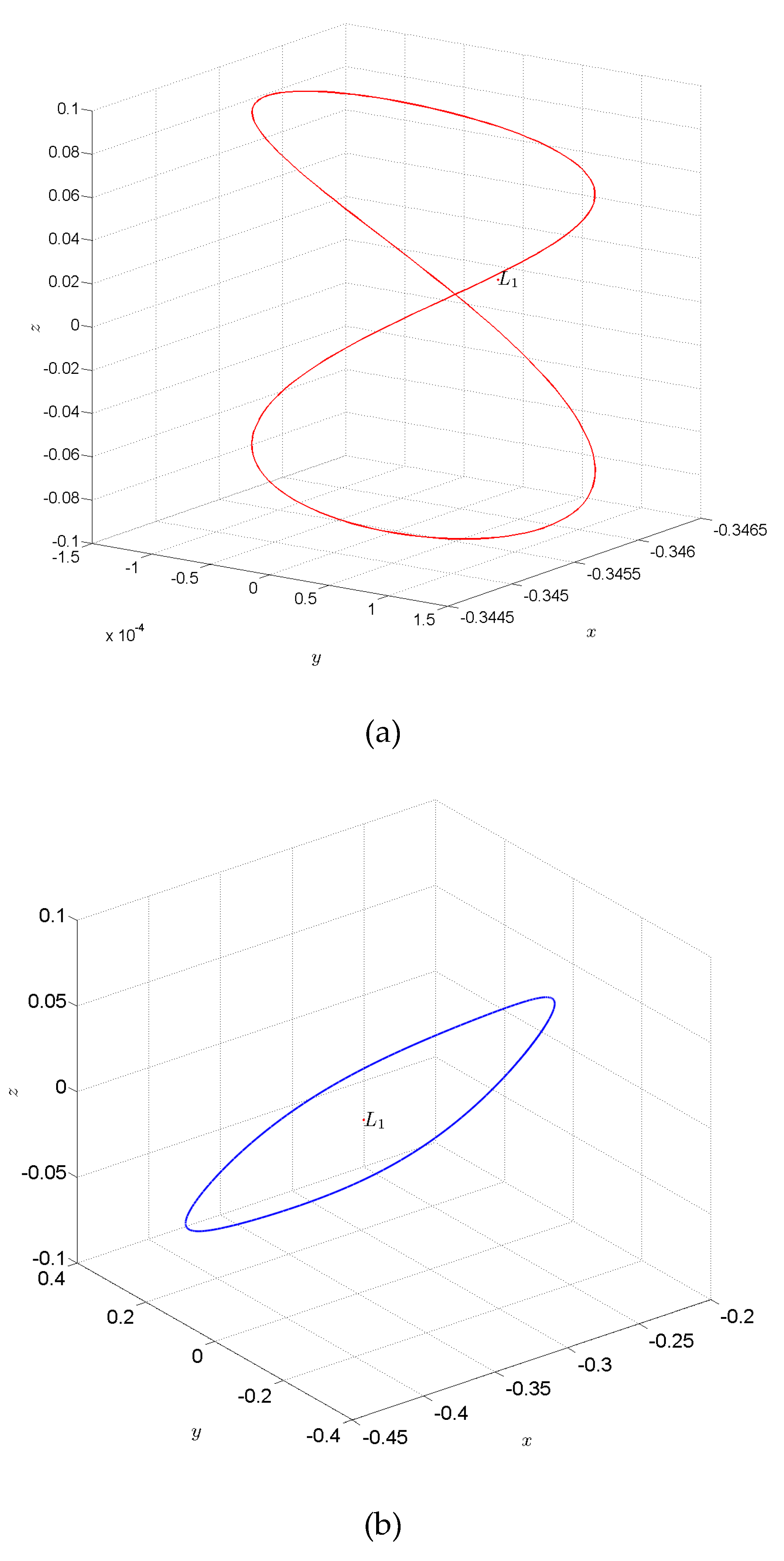
The periodic orbits around the collinear equilibrium point $L_1$ are plotted in the spatial space as shown in Figure 13. Figure 13a is a periodic orbit up to the second-order terms, and Figure 13b is a periodic orbit up to the third-order terms. Because we selected different solutions in terms of $e$, i.e., effects of various of factors of deformation, orbital vibration, and motion, there are different forms of orbits.

6. Conclusions

In this paper, we focus on constructing the approximate analytical periodic solutions of the binary HD 191408 system by using Lindstedt-Poincaré method. The obtained second- and third-order periodic solutions in the plane and three-dimensional space generalized the corresponding ones in [17].

In addition, we perform extensive numerical research on the bifurcation of the system to discuss the effects of nine perturbations on the third particle’s dynamic behavior. These nine parameters include mass ratio $\mu$, triaxial coefficients $s_i \left(i=1, 2, 3, 4\right)$, radiation factors $q_1$ and $q_2$, the modification in the Coriolis force $\alpha$, as well as the modification in the centrifugal force $\beta$. The results show that when the mass ratio parameter $\mu <0.5$, it has a greater effect on the third particle’s dynamic behavior than when $\mu >0.5$, and it has the strongest effect on the dynamic behavior of the third particle when $\mu =0.5$. Furthermore, the triaxial coefficients $s_1$ and $s_2$ have a more significant impact on the system than $s_3$ and $s_4$. This mainly reflects that the dynamic behavior of the third particle changes greatly when the system is under the joint action of $s_1$ and $s_2$, but it gradually stabilizes under the combined action of $s_3$ and $s_4$.

Furthermore, compared with the corresponding radiation factor $q_2$ and the modification in the Coriolis force $\alpha$, we also find that radiation factor $q_1$ and the modification in the centrifugal force $\beta$ have a greater impact on the dynamic behavior of the third particle, but with the increase of $q_1$ and $q_2$, the dynamic behavior of the third particle stabilizes gradually, and the same happens when $\alpha$ and $\beta$ increase together. It is hoped that the above results will help us to understand the dynamic evolution of binary system.

References

- Musielak, Z.E.; Quarles, B. The three-body problem. Rep. Prog. Phys. 2014, 77, 30. [Google Scholar] [CrossRef] [Green Version]
- Gao, F.B.; Zhang, W. A study on periodic solutions for the circular restricted three-body problem. Astron. J. 2014, 148, 116. [Google Scholar] [CrossRef] [Green Version]
- Singh, J.; Begha, J.M. Periodic orbits in the generalized perturbed restricted three-body problem. Astrophys. Space Sci. 2011, 332, 319–324. [Google Scholar] [CrossRef]
- Singh, J.; Begha, J.M. Stability of equilibrium points in the generalized perturbed restricted three-body problem. Astrophys. Space Sci. 2011, 331, 511–519. [Google Scholar] [CrossRef]
- Tsirogiannis, G.A.; Douskos, C.N.; Perdios, E.A. Computation of the Lyapunov orbits in the photogravitational RTBP with oblateness. Astrophys. Space Sci. 2006, 305, 389–398. [Google Scholar] [CrossRef]
- Singh, J.; Kalantonis, V.S.; Gyegwe, J.M.; Perdiou, A.E. Periodic motions around the collinear equilibrium points of the restricted three-body problem where the primary is a triaxial rigid body and secondary is an oblate spheroid. Astrophys. J. Suppl. 2016, 227, 1–13. [Google Scholar] [CrossRef]
- Kalantonis, V.S.; Douskos, C.N.; Perdios, E.A. Numerical determination of homoclinic and heteroclinic orbits at collinear equilibria in the restricted three-body problem with oblateness. Celest. Mech. Dyn. Astron. 2006, 94, 135–153. [Google Scholar] [CrossRef]
- Zotos, E.E. How does the oblateness coefficient influence the nature of orbits in the restricted three-body problem? Astrophys. Space Sci. 2015, 358, 1–33. [Google Scholar] [CrossRef] [Green Version]
- Elshaboury, S.M.; Abouelmagd, E.I.; Kalantonis, V.S.; Perdios, E.A. The planar restricted three-body problem when both primaries are triaxial rigid bodies: Equilibrium points and periodic orbits. Astrophys. Space Sci. 2016, 361, 315. [Google Scholar] [CrossRef]
- Jain, P.; Aggarwal, R.; Mittal, A.; Abdullah. Periodic orbits in the photogravitational restricted problem when the primaries are triaxial rigid bodies. Int. J. Astron. Astrophys. 2016, 6, 111–121. [Google Scholar] [CrossRef] [Green Version]
- Idrisi, M.J.; Ullah, M.S. Non-collinear libration points in ER3BP with albedo effect and oblateness. J. Astrophys. Astron. 2018, 39, 28. [Google Scholar] [CrossRef]
- Chen, J.J. A Bayesian Approach to the Understanding of Exoplanet Populations and the Origin of Life. Ph.D. Thesis, Columbia University, New York, NY, USA, 2018. [Google Scholar]
- Hou, X.Y.; Xin, X.S.; Feng, J.L. Forced motions around triangular libration points by solar radiation pressure in a binary asteroid system. Astrodynamics 2019. [Google Scholar] [CrossRef]
- Shi, Y.; Wang, Y.; Xu, S. Global search for periodic orbits in the irregular gravity field of a binary asteroid system. Acta Astronaut. 2019, 163, 11–23. [Google Scholar] [CrossRef]
- Howard, A.; Fulton, B. Limits on planetary companions from doppler surveys of nearby stars. Publ. Astron. Soc. Pac. 2016, 128, 114401. [Google Scholar] [CrossRef] [Green Version]
- Berardo, D.; Crossfield, I.J.M.; Werner, M.; Petigura, E.A.; Christiansen, J.; Ciardi, D.; Dressing, C.; Fulton, B.; Gorjian, V.; Greene, T.; et al. Revisiting the HIP 41378 System with K2 and Spitzer. Astron. J. 2019, 157, 185. [Google Scholar] [CrossRef] [Green Version]
- Singh, J.; Perdiou, A.; Gyegwe, J.M.; Perdios, E.A. Periodic solutions around the collinear equilibrium points in the perturbed restricted three-body problem with triaxial and radiating primaries for binary HD 191408, Kruger 60 and HD 155876 systems. Appl. Math. Comput. 2018, 325, 358–374. [Google Scholar] [CrossRef]
- Das, M.K.; Narang, P.; Mahajan, S.; Yuasa, M. Effect of radiation on the stability of equilibrium points in the binary stellar systems: RW-Monocerotis, Krüger 60. Astrophys. Space Sci. 2008, 314, 261–274. [Google Scholar] [CrossRef]
- Singh, J.; Perdiou, A.E.; Gyegwe, J.M.; Kalantonis, V.S. Periodic orbits around the collinear equilibrium points for binary Sirius, Procyon, Luhman 16, α-Centuari and Luyten 726-8 systems: The spatial case. J. Phys. Commun. 2017, 1, 025008. [Google Scholar] [CrossRef]
- Singh, J.; Umar, A. On “out of plane” equilibrium points in the elliptic restricted three-body problem with radiating and oblate primaries. Astrophys. Space Sci. 2013, 344, 13–19. [Google Scholar] [CrossRef]
- García, L.; Gómez, M. Optical polarization of solar type stars with debris disks. Rev. Mex. De Astron. Y Astrofísica 2015, 51, 1–10. [Google Scholar]
- Abia, C.; Rebolo, R.; Beckma, J.E.; Crivellari, L. Abundances of light metals and Ni in a sample of disc stars. Astron. Astrophys. 1988, 206, 100–107. [Google Scholar]
- Karaali, S.; Bilir, S.; Karatas, Y.; Ak, S.G. New metallicity calibration down to [Fe/H] = −2.75 dex. Publ. Astron. Soc. Aust. 2003, 20, 165–172. [Google Scholar] [CrossRef] [Green Version]
- Perrin, M.N. Mass estimation of twelve K dwarfs. Symp. Int. Astron. Union 1976, 72, 167–172. [Google Scholar] [CrossRef] [Green Version]
- Yumagulov, M.G.; Belikova, O.N.; Isanbaeva, N.R. Bifurcation near boundaries of regions of stability of libration points in the three-body problem. Astron. Rep. 2018, 62, 144–153. [Google Scholar] [CrossRef]
- Perdomo, O.M. A bifurcation in the family of periodic orbits for the spatial isosceles 3 body problem. Qual. Theory Dyn. Syst. 2018, 17, 411–428. [Google Scholar] [CrossRef]
- Maciejewski, A.; Rybicki, S. Global bifurcations of periodic solutions of the restricted three body problem. Celest. Mech. Dyn. Astron. 2004, 88, 293–324. [Google Scholar] [CrossRef]
- Burdge, K.; Coughlin, M.W.; Fuller, J.; Kupfer, T.; Bellm, E.C.; Bildsten, L.; Graham, M.J.; Kaplan, D.L.; Van Roestel, J.; Dekany, R.G.; et al. General relativistic orbital decay in a seven-minute-orbital-period eclipsing binary system. Nature 2019, 571, 528–531. [Google Scholar] [CrossRef] [Green Version]
- Antoniadou, K.; Libert, A.S. Spatial resonant periodic orbits in the restricted three-body problem. Mon. Not. R. Astron. Soc. 2018, 483, 2923–2940. [Google Scholar] [CrossRef]
- Antoniadou, K.I.; Voyatzis, G. Resonant periodic orbits in the exoplanetary systems. Astrophys. Space Sci. 2014, 349, 657–676. [Google Scholar] [CrossRef] [Green Version]
- Bosanac, N.; Howell, K.; Fischbach, E. Stability of orbits near large mass ratio binary systems. Celest. Mech. Dyn. Astron. 2015, 122, 27–52. [Google Scholar] [CrossRef]
- Shampine, L.F.; Reichelt, M.W. The Matlab ode suite. SIAM J. Sci. Comput. 1997, 18, 1–22. [Google Scholar] [CrossRef] [Green Version]
Figure 1.
(a–c). Bifurcation diagrams of the , , and frames in terms of mass parameter , respectively.
Figure 2.
(a–c). Bifurcation diagrams in , , and frames with respect to the triaxial coefficient , respectively.
Figure 3.
Figure 4.
(a–c). Bifurcation diagrams in , , and frames with respect to the radiation coefficient , respectively.
Figure 5.
(a–c). Bifurcation diagrams in , , and frames with respect to the Coriolis and the centrifugal force , respectively.
Figure 6.
Zero-velocity surface of the third particle C = 3.
Figure 7.
Zero-velocity surface of the third particle C = 2.914.
Figure 8.
Zero-velocity surface of the third particle C = 2.1943.
Figure 9.
Zero-velocity surface of the third particle C = 1.9777.
Figure 10.
Zero-velocity surface of the third particle C = 1.
Figure 11.
Zero-velocity curves of the third particle for C = 2.914, 2.1943, and 1.9777, respectively.