Rotating Disc around a Schwarzschild Black Hole

Simple Summary

Metric for a linear perturbation of Schwarzschild due to a rotating thin disc.

Abstract

A stationary and axisymmetric (in fact circular) metric is reviewed which describes the first-order perturbation of a Schwarzschild black-hole space-time due to a rotating finite thin disc encircling the hole symmetrically. The key Green functions of the problem (corresponding to an infinitesimally thin ring)—the one for the gravitational potential and the one for the dragging angular velocity—were already derived, in terms of infinite series, by Will in 1974, but we have now put them into closed forms using elliptic integrals. Such forms are more practical for numerical evaluation and for integration in problems involving extended sources. This last point mostly remains difficult, but we illustrate that it may be workable by using the simple case of a finite thin disc with constant Newtonian surface density.

1. Static and Stationary Sources around Black Holes

Many highly active sources in the Universe appear to be driven by black holes strongly interacting with the surrounding matter and fields. Black holes are well accessible to analytical study if they are isolated and stationary (under asymptotic flatness, such assumptions lead to the Kerr-Newman family of solutions), but otherwise it is a formidable task. There exist several special non-stationary black-hole solutions, such as those belonging to the Robinson-Trautman class, but, in general, heavy numerical codes or/and sophisticated approximation techniques have to be employed then. However, stationarity can often be assumed, since—as concerns the gravitational field—most astrophysical systems dominated by black holes remain almost stationary over considerable time periods. On the other hand, it may be problematic to assume isolation, namely to approximate the gravitational field by that solely generated by the black hole, because even a very low-mass (and moderate-density) additional source can be crucial for certain features of the field. For example, in a Schwarzschild space-time, actually any additional source dominates the tangential component of the field, simply because the original field is exactly radial. This is a rather trivial example, but such a conclusion holds quite generally for higher derivatives of the field, at least in the vicinity of the external sources;1 actually, it may already hold on the level of curvature (second derivatives of metric). The curvature, conversely, determines the stability of motion of the matter (of the matter itself which contributes to the curvature). Consequently, a (self-)gravitating matter may assume—under otherwise the “same” conditions—quite a different configuration than a test matter.

In a quasi-stationary situation, the matter flow is supposed to typically have, around astrophysical black holes, a roughly axially symmetric disc geometry. If the matter just follows circular orbits (it moves in the direction of the two space-time symmetries), the space-time is also orthogonally transitive, which means that there exist global meridional planes, everywhere orthogonal to both the Killing symmetries. The metric of such circular space-times (see e.g., [1] for a thorough account) can be written

$$\mathrm{d}{s}^2=-e^{2\nu }\mathrm{d}{t}^2+B^2{r}^2{e}^{-2\nu }{sin}^2\theta {(\mathrm{d}\varphi -\omega \mathrm{d}t)}^2+e^{2\zeta -2\nu }(\mathrm{d}{r}^2+r^2\mathrm{d}{\theta }^2),$$

(1)

where the t and $\varphi$ coordinates (time and azimuth) are adapted to the Killing symmetries, while r (called isotropic radius) and $\theta$ cover the meridional surfaces orthogonal to both Killing directions. They are related to the Weyl-type cylindrical coordinates by

$$\rho =rsin\theta ,z=rcos\theta .$$

The unknown metric functions $\nu$, B, $\omega$ and $\zeta$ only depend on r and $\theta$; they are determined by the Einstein equations. The equation for B reads, in the Weyl coordinates,

$$B_{,\rho \rho }+\frac{2B_{,\rho }}{\rho }+B_{,zz}=8\pi B(T_{\rho \rho }+T_{zz})$$

(2)

and it is being solved first in any specific situation. In a vacuum case ($T_{\mu \nu }=0$), and when a black hole (of mass M) is present, it is convenient to choose

$$B=1-\frac{M^2}{4({\rho }^2+z^2)}=1-\frac{M^2}{4r^2};$$

(3)

with such a choice, the horizon lies at $r=M/2$ (while the other common choice $B=1$ makes the horizon just a rod at $\rho =0$, $\left|z\right|\le M$, which is less convenient).

Provided that the energy-momentum tensor satisfies $T_{\rho }^{\rho }+T_z^z=0$, the remaining independent field equations can be combined to

$$\nabla ·(B\nabla \nu )-\frac{B^3{\rho }^2}{2e^{4\nu }}{(\nabla \omega )}^2=4\pi B{e}^{2\zeta -2\nu }\left(T_{\varphi }^{\varphi }-2\omega T_{\varphi }^t-T_t^t\right),$$

(4)

$$\nabla ·(B^3{\rho }^2{e}^{-4\nu }\nabla \omega )=-16\pi B{e}^{2\zeta -2\nu }{T}_{\varphi }^t,$$

(5)

$${\zeta }_{,\rho }{\left(B\rho \right)}_{,\rho }-{\zeta }_{,z}{\left(B\rho \right)}_{,z}=-B\rho \left[{\left({\nu }_{,\rho }\right)}^2-{\left({\nu }_{,z}\right)}^2\right]-\frac{1}{2}\left[{\left(B\rho \right)}_{,\rho \rho }-{\left(B\rho \right)}_{,zz}\right]+\frac{1}{4}{B}^3{\rho }^3{e}^{-4\nu }\left[{\left({\omega }_{,\rho }\right)}^2-{\left({\omega }_{,z}\right)}^2\right],$$

(6)

$${\zeta }_{,\rho }{\left(B\rho \right)}_{,z}+{\zeta }_{,z}{\left(B\rho \right)}_{,\rho }=-2B\rho {\nu }_{,\rho }{\nu }_{,z}-{\left(B\rho \right)}_{,\rho z}+\frac{1}{2}{B}^3{\rho }^3{e}^{-4\nu }{\omega }_{,\rho }{\omega }_{,z},$$

(7)

where ∇ and $\nabla ·$ denote gradient and divergence in an (auxiliary) Euclidean three-space. Appropriate boundary conditions at infinity (asymptotical flatness), at the horizon (regularity) and on the axis (absence of conical singularity) have to be added. The first two equations should be solved for $\nu$ and $\omega$, and then—with $\nu$ and $\omega$ already known—$\zeta$ can be obtained by line integration from the last two equations.

Practically, the above procedure is almost never feasible analytically, because the equations are non-linear and coupled. The only simple exception is the static case, $\omega =0$, when, outside of the sources, (4) becomes the Laplace equation. Therefore, in the static case, $\nu$ behaves exactly like the Newtonian potential; in particular, $\nu$ generated by multiple sources is obtained by linear superposition. The exercise still differs from the Newtonian one, because there is also the second metric function $\zeta$. Equations (6) and (7) simplify considerably in the static case, yet they still remain non-linear (in gradient of $\nu$) and their line integration can usually be only done numerically. However, $\zeta$ influences the meridional geometry, and it can actually deform it very strongly with respect to the corresponding (flat) Newtonian situation (described by the same $\nu$). As expected, the biggest differences arise in the vicinity of very compact sources where the gradient of $\nu$ is very large.

In the generic, stationary but non-static case, there are still two main analytical options. The first one is to use some of the generating techniques—mathematical operations which transform between metrics of the given symmetries. It is known that actually any solution can be obtained in this way, but one has little control over what comes out—most of such solutions remain unexplored, and most of them are likely to be unphysical. The second option is to perform, within the given class of metrics, a perturbation of some known solution. This route is much more straightforward, but it is only limited to small deviations from the chosen “seed” metric.2 Also, even for very simple seeds, the equations are still so complicated that it is usually impossible to reach more than a linear order.

Subject of This Paper

In the present paper, we report some recent results on perturbative treatment of circular (stationary, axisymmetric and orthogonally transitive) problem, starting from the Schwarzschild space-time as the seed. The Green functions for $\nu$ and $\omega$ were already given by Will in 1974 [2] (they correspond to the linear perturbation due to a slowly rotating and light circular ring of infinitesimal cross section). The Green functions, written there in terms of infinite series, we put into closed forms using elliptic integrals.3 Such forms are better for numerical study, but mainly they are more convenient when trying to solve problems involving extended sources (when the Green functions have to be integrated out, together with the respective density, over the source volume). We demonstrated that such an integration can in simple cases really be performed, on the example of a linear perturbation of the Schwarzschild black hole due to a constant-density finite thin circular disc extending between two concentric radii. We also showed that the solution has satisfactory properties within a reasonable parameter range, in particular, that the disc can be interpreted either as a one stream of ideal fluid or as two counter-rotating dust (geodesic) streams.

Below, we first (Section 2) write down the formulas describing the above linear perturbation, then in Section 3 we list basic properties of the solution (showing that it is physically acceptable), and finally add some comments and future options in Concluding remarks. For details of the derivation, as well as for literature, we refer to the papers [5,6].

Notation: we use geometrized units in which $c=1$, $G=1$, index-posed comma indicates partial differentiation and usual summation rule is employed. Space-time metric $g_{\mu \nu }$ has signature (−+++).

2. Metric for the Rotating-Disc Perturbation of Schwarzschild

Let us stress once more that the perturbation we consider is special in keeping the space-time circular (i.e., stationary, axisymmetric and possessing global meridional planes). The procedure is quite straightforward: we took the metric (1), chose B according to (3), expressed the other metric functions $\nu$, $\omega$ and $\zeta$ as power series in a small parameter proportional to the mass density of the perturbing source, expanded the source terms themselves in a similar way, wrote down the Einstein equations, linearized them in the perturbation quantities, found the Green functions for the perturbations of $\nu$ and $\omega$, and expressed the latter in close forms. Such forms are a natural starting point when trying to find the field of extended sources4 (by convoluting the Green functions with the source terms). Not to forget, if successful in finding the perturbed $\nu$ and $\omega$, one should also finally fix $\zeta$ by a line integral given by the gradients of (the already known) $\nu$ and $\omega$. See [5] for details.

The specific result we summarize here for illustration is the linear perturbation of Schwarzschild due to a rotating thin disc lying between two radii $r_{\mathrm{out}}>r_{\mathrm{in}}(>M/2)$. For the gravitational potential $\nu$, we employ the known formula for the potential generated by a uniform-density disc in the Newtonian theory, see [8]. It leads to the expression5

$$\nu (x,\theta )={\nu }_{\mathrm{Schw}}+V(x^{\prime }=x_{\mathrm{out}};x,\theta )-V(x^{\prime }=x_{\mathrm{in}};x,\theta ),$$

(8)

where

$${\nu }_{\mathrm{Schw}}=ln\frac{2r-M}{2r+M}$$

(9)

is the Schwarzschild part, and the potential of the disc (of constant Newtonian surface density S) reads

$$\begin{array}{cc}V(x^{\prime };x,\theta )\hfill & =2\pi MSx|cos\theta |H(x^{\prime 2}-{cos}^2\theta -x^2{sin}^2\theta )-2MS\sqrt{a_{31}{a}_{42}}E\left(k\right)-\hfill \\ & -\frac{2MS}{\sqrt{a_{31}{a}_{42}}}\left(x^{\prime 2}-{cos}^2\theta -x^2{sin}^2\theta \right)\times \hfill \\ & \times \left[K\left(k\right)+\frac{x^2{cos}^2\theta }{{\left(\sqrt{x^{\prime 2}-1}+\sqrt{x^2-1}sin\theta \right)}^2}\mathsf{\Pi }\left(\frac{4\sqrt{(x^2-1)(x^{\prime 2}-1)}sin\theta }{{\left(\sqrt{x^{\prime 2}-1}+\sqrt{x^2-1}sin\theta \right)}^2},k\right)\right],\hfill \end{array}$$

(10)

where $x:=\frac{r}{M}\left(1+\frac{M^2}{4r^2}\right)$ is a suitable dimensionless radius, $H\left(x\right)$ stands for the Heaviside function, the $a_{rs}$ and k are given by

$$\begin{array}{cc}\hfill & a_1=x{x}^{\prime }+\sqrt{(x^2-1)(x^{\prime 2}-1)},a_2=x{x}^{\prime }-\sqrt{(x^2-1)(x^{\prime 2}-1)},a_3=sin\theta ,a_4=-sin\theta ,\hfill \\ \hfill & a_{rs}=a_s-a_r,k^2=\frac{2a_{21}sin\theta }{a_{31}{a}_{42}}=\frac{4\sqrt{(x^2-1)(x^{\prime 2}-1)}sin\theta }{x^2{x}^{\prime 2}-{\left[\sqrt{(x^2-1)(x^{\prime 2}-1)}-sin\theta \right]}^2},\hfill \end{array}$$

(11)

and $K\left(k\right)$, $E\left(k\right)$ and $\mathsf{\Pi }(.,k)$ are standard complete elliptic integrals (k is their modulus, so the roots in definitions contain $k^2$).

The dragging angular velocity $\omega$ is fully given by the linear perturbation (since ${\omega }_{\mathrm{Schw}}=0$),6

$$\begin{array}{cc}{(x+1)}^3\omega (x,\theta )\hfill & =\frac{W}{2}\left[\frac{1}{{(x_{\mathrm{in}}+1)}^2}-\frac{1}{{(x_{\mathrm{out}}+1)}^2}\right]-\frac{x-1}{1+|cos\theta |}\left[\frac{x_{\mathrm{in}}}{{(x_{\mathrm{in}}+1)}^2}-\frac{x_{\mathrm{out}}}{{(x_{\mathrm{out}}+1)}^2}\right]+\hfill \\ & +\frac{W}{2\pi {sin}^2\theta }{\left[a_{41}\frac{Y_{\mathrm{K}}K\left(k\right)+Y_{\mathrm{E}}E\left(k\right)+Y_0\mathsf{\Pi }(n_0,k)+Y_1\mathsf{\Pi }(n_1,k)+Y_2\mathsf{\Pi }(n_2,k)}{{(x^{\prime }+1)}^2\sqrt{a_{31}{a}_{42}}}\right]}_{x_{\mathrm{in}}}^{x_{\mathrm{out}}},\hfill \end{array}$$

(12)

where W is a free constant (like S in the case of potential $\nu$), the factors

$$n_0=-\frac{2sin\theta }{a_{31}},n_1=-\frac{2sin\theta (a_1+1)}{a_{31}(1-sin\theta )},n_2=\frac{2sin\theta (a_1-1)}{a_{31}(1+sin\theta )}$$

represent characteristics of the $\mathsf{\Pi }(n,k)$ integrals, the “coefficients” standing at elliptic integrals read

$$\begin{array}{cc}\hfill Y_{\mathrm{K}}& =\frac{a_{31}}{a_1^2-1}\left[2x^{\prime }(x-1)(x^{\prime }{a}_1+1)+x{a}_{21}-x{x}^{\prime }(x^2-x^{\prime 2})\right],\hfill \\ \hfill Y_{\mathrm{E}}& =\frac{x^{\prime }(x-2)a_{31}{a}_{42}}{a_{41}},\hfill \\ \hfill Y_0& =-2(x-1)(x^{\prime 2}+1)-2{sin}^2\theta ,\hfill \\ \hfill Y_1& =-\frac{(x-1){(x^{\prime }-1)}^2(x+x^{\prime })(1+sin\theta )}{a_1+1},\hfill \\ \hfill Y_2& =\frac{(x-1){(x^{\prime }+1)}^2(x-x^{\prime })(1-sin\theta )}{a_1-1},\hfill \end{array}$$

(13)

and the evaluation at the disc edges has been denoted by ${\left[X\right]}_{x_{\mathrm{in}}}^{x_{\mathrm{out}}}=X(x^{\prime }=x_{\mathrm{out}})-X(x^{\prime }=x_{\mathrm{in}})$.

Finally, the last metric function $\lambda$ can only be found numerically. The easiest way is to write down the relevant Einstein equations in the Weyl coordinates ($\rho$, z) and with the choice $B=1$. In vacuum and in the linear perturbation order (when the function $\omega$ does not enter at all), they are the same as in the static case,

$$\begin{array}{c}\hfill {\lambda }_{,\rho }=\rho \left[{\left({\nu }_{,\rho }\right)}^2-{\left({\nu }_{,z}\right)}^2\right],{\lambda }_{,z}=2\rho {\nu }_{,\rho }{\nu }_{,z}.\end{array}$$

These equations are solved by a line integration going from the axis (where $\lambda =lnB$ necessarily, so for $B=1$ it vanishes) to a given location along any path going through a vacuum region. However, in order to be consistent with the above results, one then has to adapt the solution to our choice $B=1-\frac{M^2}{4r^2}$. This is done according to the transformation (see [5], Equation (80); note that the first expression for $\tilde{\rho }$ was given there with a wrong sign)

$$\begin{array}{cc}\hfill \tilde{\rho }& =\frac{\rho (4{\rho }^2+4z^2-M^2)}{4({\rho }^2+z^2)}=\frac{(4r^2-M^2)sin\theta }{4r}=M\sqrt{x^2-1}sin\theta ,\hfill \\ \hfill \tilde{z}& =\frac{z(4{\rho }^2+4z^2+M^2)}{4({\rho }^2+z^2)}=\frac{(4r^2+M^2)cos\theta }{4r}=Mxcos\theta ,\hfill \\ \hfill \tilde{\lambda }& =\lambda -\frac{1}{2}ln\frac{{(4{\rho }^2+4z^2+M^2)}^2-16M^2{z}^2}{16{({\rho }^2+z^2)}^2}=\lambda -\frac{1}{2}ln\frac{{(4r^2+M^2)}^2-16r^2{M}^2{cos}^2\theta }{16r^4}=\hfill \\ \hfill & =\lambda -\frac{1}{2}ln\frac{4(x^2-{cos}^2\theta )}{{\left(x+\sqrt{x^2-1}\right)}^2},\hfill \end{array}$$

(14)

where tilded quantities correspond to $B=1$ and untilded quantities to $B=1-\frac{M^2}{4r^2}$.

3. Basic Properties of the Solution

3.1. Mass and Angular Momentum

Let us list basic properties of the above linear-perturbation solution. The mass and angular momentum can either be found by computing the respective Komar integrals, or from behaviour of the metric functions at radial infinity. Both methods yield the same results, in particular, the metric functions fall off asymptotically $(r\to \infty )$ as

$$\nu \propto -\frac{M+\mathcal{M}}{r},\omega \propto \frac{2\mathcal{J}}{r^3},\zeta \propto -\frac{M^2}{4r^2}$$

(15)

(the last relation can easily be obtained on the symmetry axis where $e^{\zeta }=B$ must hold), where

$$\mathcal{M}=\pi S\left[r_{\mathrm{out}}^2-r_{\mathrm{in}}^2-\frac{M^4}{16}\left(\frac{1}{r_{\mathrm{in}}^2}-\frac{1}{r_{\mathrm{out}}^2}\right)\right],\mathcal{J}=\frac{W{M}^2}{8}\left[r_{\mathrm{out}}-r_{\mathrm{in}}-\frac{M^2}{4}\left(\frac{1}{r_{\mathrm{in}}}-\frac{1}{r_{\mathrm{out}}}\right)\right]$$

(16)

represent the disc contributions, while the black-hole mass remains M and the black-hole angular momentum remains zero. In spite of the latter, the horizon does rotate with respect to infinity with non-zero angular velocity,

$${\omega }_{\mathrm{H}}=\frac{W}{8}\frac{(x_{\mathrm{out}}-x_{\mathrm{in}})(x_{\mathrm{out}}+x_{\mathrm{in}}+2)}{{(x_{\mathrm{out}}+1)}^2{(x_{\mathrm{in}}+1)}^2};$$

(17)

this means that the black hole is just being dragged along by the rotational effect of the disc.

3.2. Horizon Geometry

Whenever a black hole is under the (gravitational) influence of some other source, it is interesting to check how affected is the geometry of the horizon (understood as a 2D surface, namely its $t=\mathrm{const}$ section). Actually, with the choice $B=1-\frac{k^2}{4r^2}$, the black-hole horizon stays at $r=\frac{M}{2}$, so its coordinate picture is exactly spherical irrespectively of the perturbation, yet the intrinsic shape of the horizon (given by proper distances in the two angular directions) does change due to the presence of the additional source. In our case, we showed that—in agreement with common experience—the horizon inflates towards the encircling disc, i.e., it becomes oblate. If the disc density (S) is sufficiently large, and/or if the disc is sufficiently extended, the horizon can even be deformed so strongly that its Gauss curvature becomes negative (first at the axis).7

The horizon area and surface gravity come out

$$A_{\mathrm{H}}=16\pi M^2{e}^{-2{\nu }_1(x=1,\theta =0)}=16\pi M^2{e}^{4\pi MS(x_{\mathrm{out}}-x_{\mathrm{in}})},{\kappa }_{\mathrm{H}}=\frac{4\pi M}{A_{\mathrm{H}}}.$$

(18)

Note that this result is independent of $\theta$, that is, ${\kappa }_{\mathrm{H}}$ is uniform all over the horizon, in agreement with the zeroth law of black-hole thermodynamics. We see that the horizon area grows (exponentially) while the surface gravity weakens with the increase of the disc density S.

3.3. Static Limit and Singularity

A rotating horizon is usually surrounded by a static limit—a surface which limits the possibility to stay at rest relative to an asymptotic rest frame (namely to “resist” rotational dragging caused by the source). It is given by $g_{tt}=0$. In a non-rotating case, the static limit coincides with the horizon. We showed that our first-order perturbation does not separate a static limit from the horizon, so there does not appear any ergosphere. Similarly, we also checked, by analysing the Kretschmann scalar (square of the Riemann tensor), that the physical singularity inside the black hole keeps its original, point-like character (and does not turn ring-like as is the case for the Kerr black hole).

3.4. Circular Motion in the Black-Hole + Disc Field

The disc influence naturally reveals the properties of test motion. A default first check is the stationary motion along circular orbits, i.e., the motion which just follows the given space-time symmetries. One can for example ask about light-like limits of circular motion, about conditions for free (geodesic) circular motion, about zero-speed limit of free circular motion,8 about the locations of photon (light-like), marginally stable and marginally bound circular geodesics. We will not list all these properties here, since the explicit forms of the corresponding conditions (specific to our system) are rather cumbersome; they can be found in [6], including illustrations. However, the circular motion is interesting in that it “feels” the rotational perturbation already in the linear order—namely, the respective conditions typically contain the dragging angular velocity $\omega$ linearly.

3.5. Interpretation of the Disc

One of the most important questions is whether the resulting general relativistic solution can really be interpreted as describing the field of a black hole encircled by a thin disc with physically acceptable properties. There are two main options how to interpret the disc matter: (i) as a one stream of ideal fluid characterized by proper surface density $\sigma$, proper azimuthal pressure P and orbital velocity v (thus being kept on its circular orbits by a combination of gravitational, inertial and pressure effects); (ii) as two counter-rotating geodesic (i.e., non-interacting, pressureless) streams characterized by their proper densities ${\sigma }_{\pm }$ and velocities $v_{\pm }$. As derived in [5], these parameters are given by

$$\begin{array}{cc}\hfill {\sigma }_{\pm }& =\frac{4r^2-8Mr+M^2}{8r^2}\left[S\pm \frac{W{\left(Mr\right)}^{3/2}}{2\pi {(2r+M)}^3}\right],\hfill \end{array}$$

(19)

$$\begin{array}{cc}\hfill v_{\pm }& =\pm v_0:=\pm \frac{2\sqrt{Mr}}{2r-M};\hfill \end{array}$$

(20)

$$\begin{array}{cc}\hfill \sigma & =+\frac{{\sigma }_{+}+{\sigma }_{-}}{2}+\sqrt{{\left(\frac{{\sigma }_{+}+{\sigma }_{-}}{2}\right)}^2+\frac{4{\sigma }_{+}{\sigma }_{-}{v}_0^2}{{(1-v_0^2)}^2}}=\hfill \end{array}$$

$$\begin{array}{cc}\hfill & =+\frac{{\sigma }_{+}+{\sigma }_{-}}{2}+\sqrt{{\left(\frac{{\sigma }_{+}+{\sigma }_{-}}{2}\right)}^2+\frac{16Mr{(2r-M)}^2{\sigma }_{+}{\sigma }_{-}}{{(4r^2-8Mr+M^2)}^2}},\hfill \\ \hfill P& =-\frac{{\sigma }_{+}+{\sigma }_{-}}{2}+\sqrt{{\left(\frac{{\sigma }_{+}+{\sigma }_{-}}{2}\right)}^2+\frac{4{\sigma }_{+}{\sigma }_{-}{v}_0^2}{{(1-v_0^2)}^2}}=\hfill \end{array}$$

(21)

$$\begin{array}{cc}\hfill & =-\frac{{\sigma }_{+}+{\sigma }_{-}}{2}+\sqrt{{\left(\frac{{\sigma }_{+}+{\sigma }_{-}}{2}\right)}^2+\frac{16Mr{(2r-M)}^2{\sigma }_{+}{\sigma }_{-}}{{(4r^2-8Mr+M^2)}^2}},\hfill \end{array}$$

(22)

$$\begin{array}{cc}\hfill v^2& =\frac{\sigma v_0^2-P}{\sigma -P{v}_0^2}=\frac{4Mr\sigma -{(2r-M)}^{2}P}{{(2r-M)}^2\sigma -4MrP}.\hfill \end{array}$$

(23)

Note that in obtaining v from the last expression, the square root has to be taken with $+/-$ sign in case that ${\sigma }_{+}>{\sigma }_{-}$/${\sigma }_{+}<{\sigma }_{-}$. Note also that $v_{\pm }$ are given by their pure-Schwarzschild values (they represent linear velocities with respect to the local zero-angular-momentum observer).

The above can be summarized as follows (see [5] for details again): the metric we derived possesses non-zero jumps across the equatorial plane within the range $(x_{\mathrm{in}},x_{\mathrm{out}})$. Using the Einstein equations, these jumps correspond to a surface energy-momentum tensor which can be written either as due to a one stream of ideal fluid with parameters $\sigma$, P and v, or as due to two freely counter-orbiting streams of dust with parameters ${\sigma }_{\pm }$ and $v_{\pm }$ (all these components are in steady circular motion). In order that such an interpretation be really plausible, the parameters have to satisfy several physical conditions.

The first are energy conditions for the energy-momentum tensor. We required the weak, the dominant and the strong energy conditions, and we found that (i) the one-stream parameters have to satisfy $\sigma \ge \left|P\right|$, (ii) the two-stream densities ${\sigma }_{\pm }$ have to be non-negative. Together with the natural requirement $P\ge 0$ (non-negative azimuthal pressure), we thus have

$$\sigma \ge P\ge 0,{\sigma }_{\pm }\ge 0.$$

By analysing the formulae for the above quantities, one finds that ${\sigma }_{\pm }\ge 0$ actually implies the first requirements, and that ${\sigma }_{\pm }$ may only become negative at $r<(1+\sqrt{3}/2)M\doteq 1.866M$ (plus ${\sigma }_{-}$ might also become negative if W were too large relative to S).

The second major physical requirement is that the matter of the disc move with subluminal speed. For both interpretations, this simply implies that the matter (or its respective component) has to only exist above the respective photon circular geodesic, i.e., that the disc must not lie too close to the horizon. Note finally that if the disc solution was considered in astrophysical models, one should, in addition, restrict to such radii where the circular motion is stable.

3.6. Illustrations

A number of illustrations have already been given in the original papers. In [5], we plotted the meridional behaviour of the total potential $\nu$ and of the dragging angular velocity $\omega$, and the radial profiles of the parameters corresponding to the one-stream and two-stream interpretations of the disc. Since the potential $\nu$ superposes exactly like in the Newtonian case (or like in static axisymmetric case in general relativity), we think it is rather worth to repeat here the other two, “non-trivial” graphs—see Figure 1 and Figure 2.

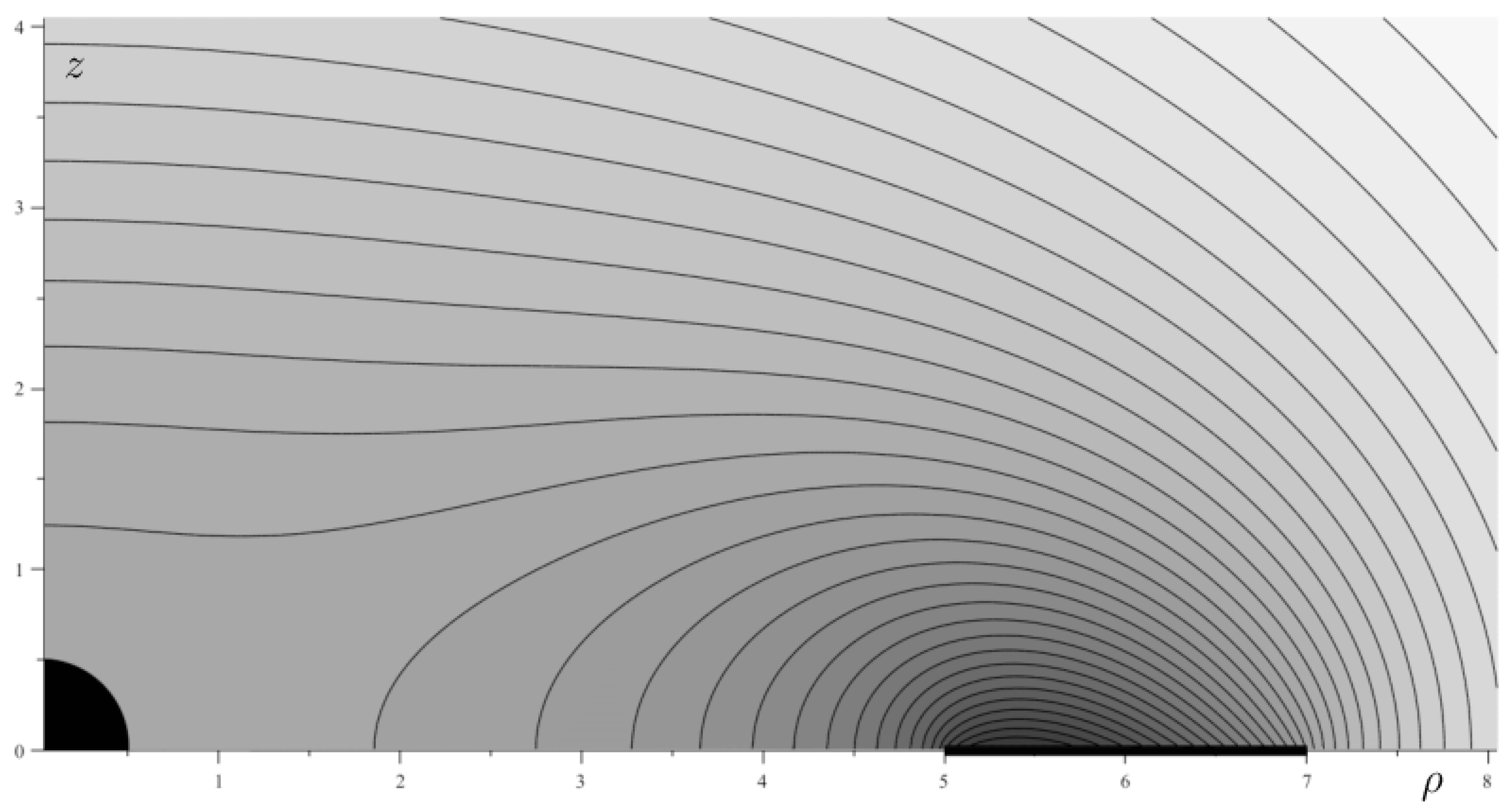
Figure 1 shows that the dragging angular velocity decreases when receding from the disc, while staying rather constant in the inner region containing the black hole. It behaves reasonably, including at the very disc ($\theta =\pi /2$, $r_{\mathrm{in}}<r<r_{\mathrm{out}}$) where its normal gradient stays finite, namely

$$\underset{\theta \to {\frac{\pi }{2}}^{-}}{lim}\frac{\partial {\omega }_1}{\partial \theta }\left(=-r\underset{z\to 0^{+}}{lim}\frac{\partial {\omega }_1}{\partial z}\right)=\frac{W}{2}\frac{x-1}{{(x+1)}^3}=8W{M}^2{r}^2\frac{{(2r-M)}^2}{{(2r+M)}^6}.$$

(24)

As it is common with thin layers, the only irregularity is in radial gradient at the disc edges.

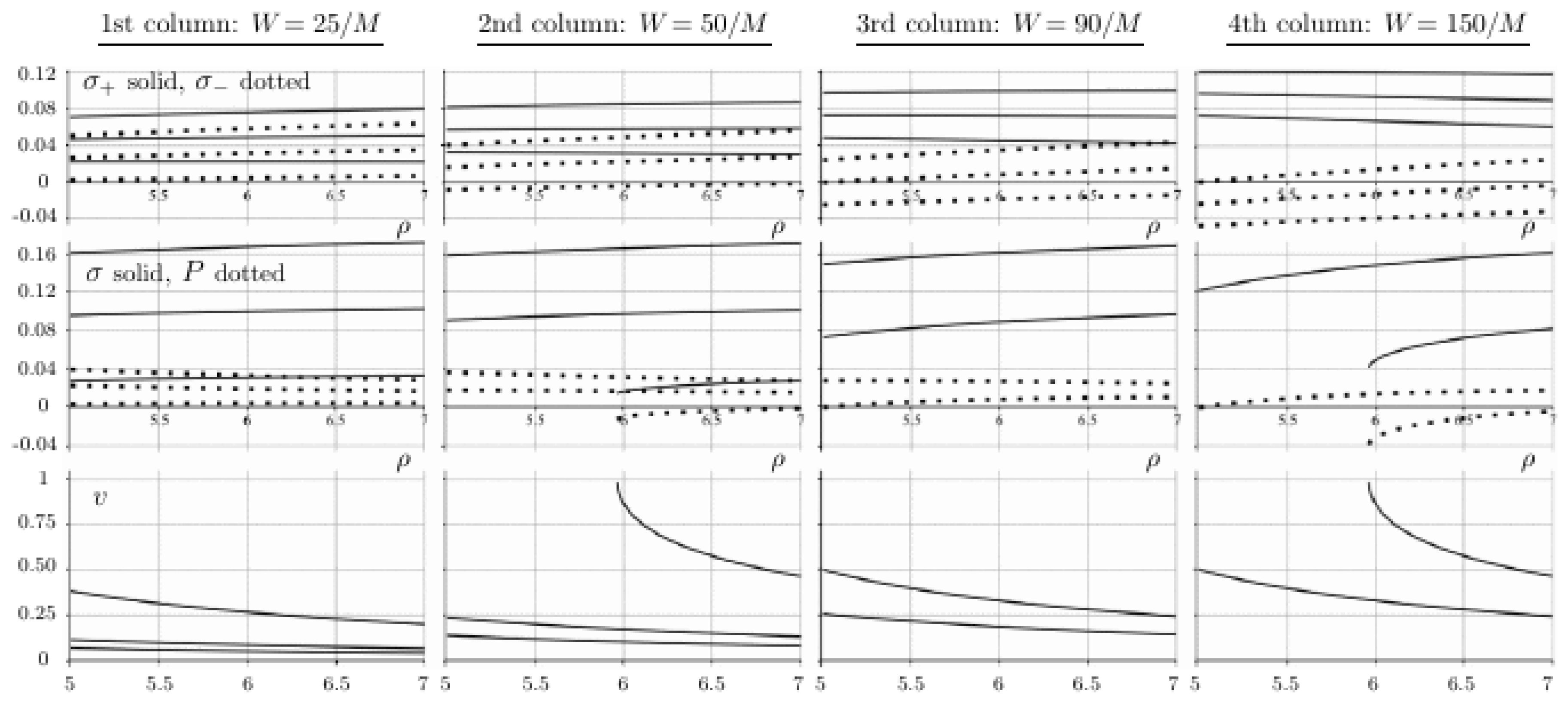
Figure 2 illustrates radial profiles of the quantities employed in the one-stream and two-stream interpretations of the disc. It is seen that both these interpretations are viable if the parameters S and W are not too large (see the figure caption for details).

4. Concluding Remarks

4.1. Validity of the Linear Approximation

Linear-perturbation approximation means that one neglects all terms quadratic and higher-order in the perturbation of $\nu$ and $\omega$ as well as in any of their derivatives. Validity of such a result is, roughly speaking, restricted to regions where the perturbations of $\nu$ and $\omega$ as well as their derivatives are small with respect to the unperturbed potential ${\nu }_{\mathrm{Schw}}$. Whether this holds depends on where the disc is placed—at large radii where the black-hole influence is already weak, even a very low values of the densities S and/or W can make the disc effect dominant, mainly in its vicinity. However, one is rather motivated by astrophysical accretion discs which are supposed to have their inner radii around or somewhat below $10M$.

In [6], we gave a rough observation for a disc lying between $r_{\mathrm{in}}=5M$ and $r_{\mathrm{out}}=8M$ (which is just above the pure-Schwarzschild innermost stable circular orbit). In such a configuration, the linear approximation is valid up to some $S\simeq 0.002/M$ and up to some $W\simeq 20/M$: for such values, the disc potential and the dragging function are at worst (close to the disc) about $3\times$ smaller than ${\nu }_{\mathrm{Schw}}$ (in magnitudes of course), so the neglected quadratic terms are at least $10\times$ smaller. To have an idea, the $5M<r<8M$ disc with $S\simeq 0.002/M$ and $W\simeq 20/M$ has mass about ${\mathcal{M}}_1\simeq 0.25M$ and angular momentum about ${\mathcal{J}}_1\simeq 7.45M^2$.

It is important to also check the gradient of $\omega$, because it is the gradient squared through which $\omega$ enters the equation for $\nu$, see (4). Besides that, one should be cautious if using higher (than the first) derivatives of $\omega$, because dragging generally falls off much faster than potential when receding from the source, so these derivatives do not tend to be small, at least close to the disc (especially close to its edges).

4.2. Outlook

It would of course be desirable to proceed to quadratic perturbation order, where only the self-gravitation occurs. In particular, only then $\omega$ “back-reacts” on $\nu$ (through its gradient squared). Unfortunately, it is almost hopeless to achieve, analytically, the quadratic approximation.

Another possible extension would be to consider a disc with different-than-constant surface density. However, one can hardly hope to be able to integrate out, together with the Green functions, anything else than just very special density profiles.

Even without further generalizations, the above metric for a Schwarzschild black hole encircled by a light rotating thin disc could now be applied (and thus further studied) in various ways. First, we plan to analyse in it the geodesic dynamics, in order to learn how the dynamics is affected by dragging. Namely, the long-term tendencies of the geodesic flow—in particular its possible tendency to chaos—are very sensitive to details of the gravitational field and, at the same time, astrophysically important. We have been studying the geodesic chaos induced by a disc within (exact) static axially symmetric setting (thus without rotation), see, e.g., [9] for a recent state of our series. It will be interesting to see how the observations made there can be perturbed by dragging, the more so that rather an attenuation of chaos (due to dragging) seems to be reported in the literature. In any case, in order to solve any problem with geodesic chaos, one should describe the gravitational field as accurately as possible. In this respect, and regarding that no appropriate exact solution is available, we would trust the above “proper perturbation” more than any approximation based on weak-field expansion of the Kerr metric.

The hole-plus-disc metric might also be applied directly—to model a gravitational field of some cosmic systems. For instance, it has recently been claimed [10] that the rotational curve of our Galaxy (known with considerably better precision now thanks to the Gaia satellite mission) could be fitted, equally well as by Newtonian dynamics in the field of a disc supplemented by the dark-matter halo, within the general relativistic picture based on the Kerr metric. However, regarding the fast fall off with distance of the dragging effects, one would estimate that for stars orbiting at large radii, rotation of the central body (the supermassive black hole in the Galaxy case) is less important than dragging generated by the rotating galactic disc itself. The above reviewed metric might be an option in this direction, since it represents the dragging due to the disc reasonably (although the disc we considered has constant Newtonian surface density which is not the case for galaxies).

Otherwise, the reviewed metric might in general be employed as describing a possible space-time background for studying various physics connected with black holes accompanied by accretion discs. It is a more complicated background than the pure Schwarzschild or Kerr one, so one cannot expect to have similar analytical possibilities, and it is only reasonably applicable for low-mass (or slowly rotating) discs, but it should still be worth to use it in studying such effects in which both the mass and rotation of the disc (i.e., the latter’s influence on both the gravitational potential and dragging) could be important at the same time. In particular, the knowledge of Green’s functions of the gravitational problem should suggest the corresponding electromagnetic ones. Actually, a disc carrying an azimuthal current and thus generating a magnetic field is the case of clear astrophysical interest.

References

- Heusler, M. Black Hole Uniqueness Theorems; Cambridge University Press: New York, NY, USA, 1996. [Google Scholar]
- Will, C.M. Perturbation of a Slowly Rotating Black Hole by a Stationary Axisymmetric Ring of Matter. I. Equilibrium Configurations. Astrophys. J. 1974, 191, 521–532. [Google Scholar] [CrossRef]
- Bach, R.; Weyl, H. Neue Lösungen der Einsteinschen Gravitationsgleichungen. B. Explizite Aufstellung statischer axialsymmetrischer Felder. Math. Zeit. 1922, 13, 134–145, reprinted in Gen. Relativ. Grav. 2012, 44, 817–832. [Google Scholar] [CrossRef]
- Semerák, O. Static axisymmetric rings in general relativity: How diverse they are. Phys. Rev. D 2016, 94, 104021. [Google Scholar] [CrossRef] [Green Version]
- Čížek, P.; Semerák, O. Perturbation of a Schwarzschild black hole due to a rotating thin disk. Astrophys. J. Suppl. 2017, 232, 14. [Google Scholar] [CrossRef] [Green Version]
- Kotlařík, P.; Semerák, O.; Čížek, P. Schwarzschild black hole encircled by a rotating thin disc: Properties of perturbative solution. Phys. Rev. D 2018, 97, 084006. [Google Scholar] [CrossRef] [Green Version]
- Geroch, R.; Traschen, J. Strings and other distributional sources in general relativity. Phys. Rev. D 1987, 36, 1017. [Google Scholar] [CrossRef] [PubMed]
- Lass, H.; Blitzer, L. The gravitational potential due to uniform disks and rings. Celest. Mech. 1983, 30, 225–228. [Google Scholar] [CrossRef]
- Polcar, L.; Suková, P.; Semerák, O. Free Motion around Black Holes with Disks or Rings: Between Integrability and Chaos–V. Astrophys. J. 2019, 877, 16. [Google Scholar] [CrossRef] [Green Version]
- Crosta, M.; Giammaria, M.; Lattanzi, M.G.; Poggio, E. Testing Dark Matter and Geometry Sustained Circular Velocities in the Milky Way with Gaia DR2. Available online: https://arxiv.org/abs/1810.04445 (accessed on 2 February 2020).