Effects of Atomic-Scale Electron Density Profile and a Fast and Efficient Iteration Algorithm for Matter Effect of Neutrino Oscillation

Abstract

In a recent article, we noticed that the electron density in condensed matter exhibits large spikes close to the atomic nuclei. We showed that the peak magnitude of these spikes in the electron densities, 3–4 orders larger than the average electron plasma density in the Sun’s core, have no effect on the neutrino emission and absorption probabilities or on the neutrinoless double beta decay probability. However, it was not clear if the effect of these spikes is equivalent to that of an average constant electron density in matter. We investigated these effects by a direct integration of the coupled Dirac equations describing the propagation of flavor neutrinos into, through, and out of the matter. We proposed a new iteration-based algorithm for computing the neutrino survival/appearance probability in matter, which we found to be at least 20 times faster than some direct integration algorithms under the same accuracy. With this method, we found little evidence that these spikes affect the standard oscillations probabilities. In addition, we show that the new algorithm can explain the equivalence of using average electron densities instead of the spiked electron densities. The new algorithm is further extended to the case of light sterile neutrinos.

1. Introduction

The results of the solar and atmospheric neutrino oscillation experiments were recognized by a recent Nobel prize. The Mikheyev–Smirnov–Wolfenstein (MSW) effect is an essential component needed for the interpretation of these neutrino oscillation experiments [1,2] (for a historical account of neutrino oscillations in matter, see [3]). Therefore, the mixing of the neutrino mass eigenstates in vacuum and in dense matter seem to be well established in describing the propagation of neutrinos from source to detecting devices. These effects were mostly considered in electron plasma [4,5], such as the Sun or supernovae, and their use is extended to condensed matter, such as the Earth crust and inner layers [6,7,8]. However, to our best knowledge, the variation of the electron density inside condensed matter has not yet been considered. A simple estimate of the electron density and neutrino potential inside a medium-Z nucleus, such as ${}^{28}$Si, shows that it is more than two orders of magnitude larger than that existing in the Sun’s core [9,10]. One could then ask if these high electron densities can produce additional mixing of the mass eigenstates that need to be considered in the interpretation of neutrino production and detection phenomenology.

The effect of the matter-induced neutrino potential on the neutrino mixing in matter is traditionally analyzed using the local in-medium mass eigenstates with modified effective masses and mixings [11,12,13]. This approach relies on the separation of the neutrino wavelength scale from the much larger neutrino oscillation and matter density variation scales. In reality, there are no such local mass eigenstates in matter (the neutrino potential is a timelike component of a vector and modifies the energy but not the mass), but the analysis of the evolution of the vacuum mass eigenstates in finite matter medium is complicated by the various scales involved. However, the results based on local, in-medium, mass eigenstates seem to be valid. One of the issues related to the introduction of the fictitious in-matter mass eigenstates is that one assumes that the neutrinos produced via weak interactions in dense matter (e.g., in the Sun’s core) are emitted as in-matter mass eigenstates. The transition to vacuum is usually described by the long-scale evolution of the amplitudes (for an example, see Reference [14]), which may or may not be adiabatic. In this article, we investigate if the results of this approach (see also Reference [9]) can be extended to the analysis of the effects of nonadiabatic transitions of the neutrinos through condensed matter, where the electron densities near the atomic nuclei are orders of magnitude larger than those in the Sun’s core. In our analysis, we use the evolution of the flavor amplitudes (see Equation (11) below), thus avoiding the complicated evolution of the fictitious in-medium mass eigenstates.

2. Neutrino Oscillations in Condensed Matter

It is now widely accepted that the flavor neutrinos participating in the weak interaction are coherent superpositions of vacuum mass eigenstates. For the neutrino fields, the mixing reads:

$${\nu }_{\alpha L}\left(x\right)=\sum _{j=1}^{N_m}{U}_{\alpha j}{\nu }_{jL}\left(x\right),$$

(1)

where index $\mathsf{\alpha }$ indicates a flavor state (electron, muon, tau, …), j designates mass eigenstates (1, 2, 3, …, $N_m$), and $U_{\mathsf{\alpha }j}$ are elements of the vacuum neutrino mixing (PMNS) matrix. Here, the dots indicate sterile flavors, or high mass eigenstates, with $N_m$ being the number of mass eigenstates. If one discards the existence of the low-mass sterile neutrinos, the coupling to the higher mass eigenstates is then very small, and the sum over j in Equation (1) is reduced to $N_m=3$. This mixing leads to violations of the flavor number, and it is reflected in the outcome of the neutrino oscillation experiments. These experiments are mostly analyzed in terms of neutrino states:

$$|{\nu }_{\alpha L}\rangle =\sum _{j=1}^3{U}_{\alpha j}^{*}|{\nu }_{jL}\rangle ,$$

(2)

which are dominated by the larger components of the fields. Neutrino states are used to analyze the matter effects, also known as Mikheyev–Smirnov–Wolfenstein effects [15]. Neutrino mixing is affected in matter by the neutrino optical potential. The general relation between the neutrino optical potential (in $eV$) and the electron density $N_e$ (in cm${}^{-3}$) is:

$$V_e\left(eV\right)=\pm \sqrt{2}{G}_F{N}_e\approx \pm 7.56\times {10}^{-14}{m}_p{N}_e=\pm 1.26\times {10}^{-37}{N}_e,$$

(3)

where the minus–plus sign corresponds to (anti)neutrinos, $G_F$ is Fermi’s constant, and $m_p$ is the proton mass ($1.67\times {10}^{-24}$ g). Above, we used Equation (2.8) of [13], where the equivalent matter density times the electron fraction $Y_e$ was replaced with $m_p{N}_e$. In atoms, just considering the electron density of two electrons in the lowest $1s$ state of a Hydrogen-like atom (the higher s-states contribute very little, $\propto 1/n^3$, n being the principal quantum number), one gets:

$$N_e\left(r\right)={10}^{30}\frac{2}{\pi }{\left(\frac{Z}{53}\right)}^3{e}^{-2rZ/53}(\mathrm{cm}{}^{-3}),$$

(4)

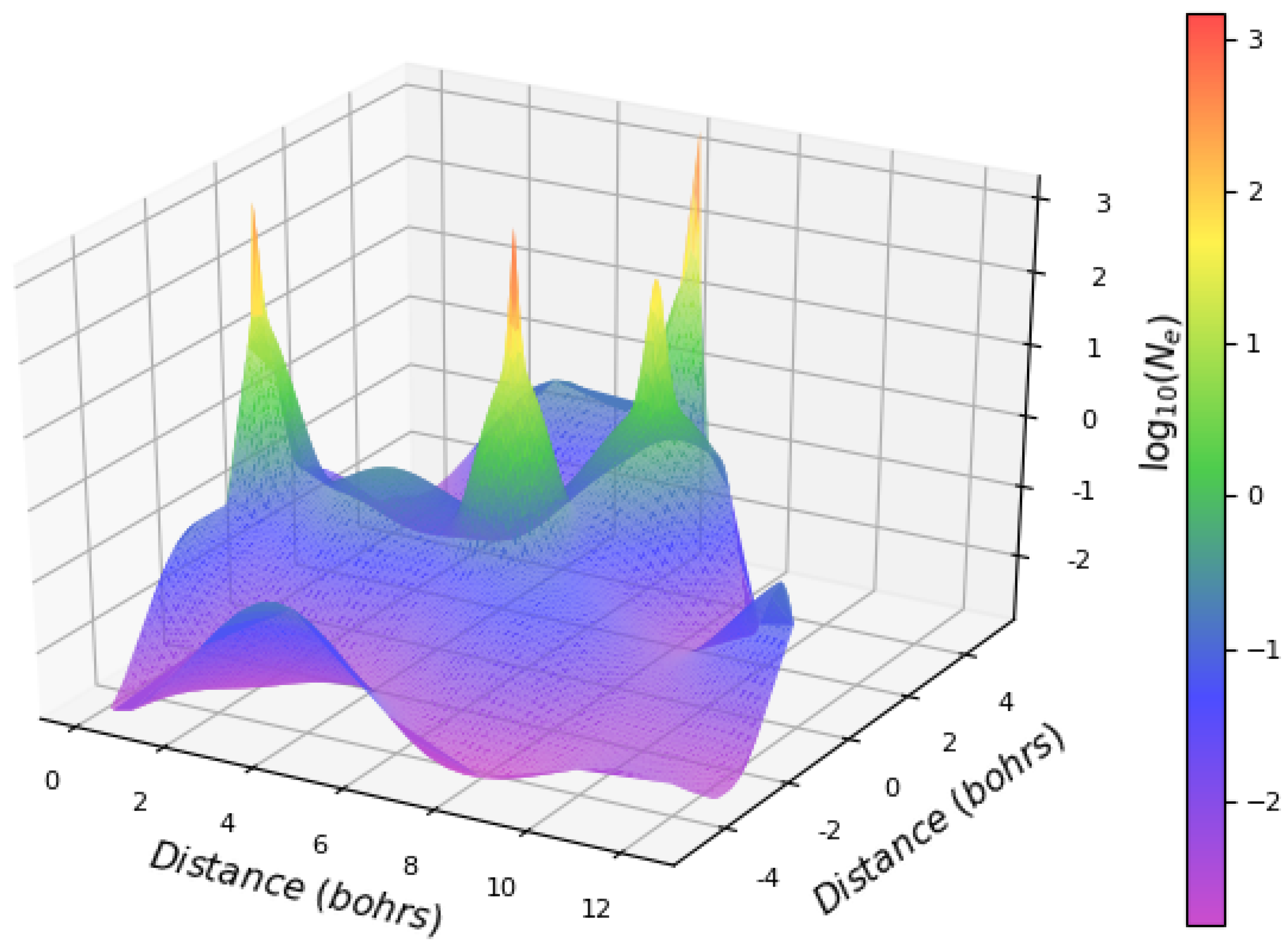
where Z is the atomic number and r is the radial distance from the atomic nuclei in pm (${10}^{-12}$ m). Electron Density Functional Theory (DFT) calculations [16,17] (for example, see Figure 1 of Reference [9]) show that this approximation is very good at and near the nuclei, where the main transition takes place. Figure 1 shows the result of a DFT calculation for the electron density in the cell of quartz crystal, one of the most common in the Earth’s crust. The results show that 85% of the electron density in the cell resides in the spikes (defined as larger than the average density of 0.1 atomic units), while only 15% is located in the volume that has lower-than-average density. In addition, the values of the electron density near the peaks are very well described by Equation (4). These high electron densities near the nuclei are much larger than those in the Sun’s core for all atoms with an atomic number greater than 5. As an example, for atoms with $Z\approx 53$, the electron density at the nucleus is four orders of magnitude larger than that in the Sun’s core.

Therefore, it should be interesting to investigate the effects of these large electron densities on the neutrino mixing in atomic weak interactions. To solve this problem, one needs to consider the evolution of mixing for three (or more) neutrino mass eigenstates, which can be described by the coupled Dirac equations:

$$i\frac{d}{dt}\left(\begin{array}{c}{\psi }_1\\ {\psi }_2\\ {\psi }_3\end{array}\right)=\left[\left(\begin{array}{ccc}{p}_x{\alpha }_x+m_1\beta & 0& 0\\ 0& p_x{\alpha }_x+m_2\beta & 0\\ 0& 0& p_x{\alpha }_x+m_3\beta \end{array}\right)+U^{†}\left(\begin{array}{ccc}{V}_e\left(x\right)+V_N\left(x\right)& 0& 0\\ 0& V_N\left(x\right)& 0\\ 0& 0& V_N\left(x\right)\end{array}\right)U\right]\left(\begin{array}{c}{\psi }_1\\ {\psi }_2\\ {\psi }_2\end{array}\right),$$

(5)

where ${\psi }_j$ are Dirac spinors for the (perturbed) vacuum mass eigenstates, $m_j$ are the corresponding neutrino masses, $p_x$ is the momentum in the direction of the beam, and ${\mathsf{\alpha }}_x$ and $\mathsf{\beta }$ are Dirac matrices [19]. Here, $V_n$ is the neutral current potential generated mostly by neutrons, i.e.,

$$V_n\left(eV\right)\approx \mp G_F{N}_n/\sqrt{2}\approx \mp 6.3\times {10}^{-38}{N}_n,$$

(6)

where $N_n$ is the local neutron density in cm${}^{-3}$ (here and below we neglect the neutral current contributions from protons and electrons, which cancel out in the limit of average constant densities). The neutral current potential is the same for all three active neutrinos, and therefore can be neglected in the analysis of neutrino oscillations (as is the main momentum term in the underlying Dirac equations). However, if the sterile neutrinos are present, the neutral current potential needs to be considered [20].

In Equation (5), the Dirac spinors ${\psi }_j={\nu }_j{\varphi }_j$ can be viewed as components of some flavor neutrino normalized superposition of mass eigenstates spinors:

$${\psi }_{\alpha }=\sum _{j=1,2,3}{\psi }_j=\sum _{j=1,2,3}{\nu }_j{\varphi }_j,$$

(7)

where $\alpha$ indicates the known active neutrino flavors—electron, muon, and tau. Here, we consider the traditional approach [14] of separating the neutrino wavelength scale from the neutrino oscillation and matter density variation scales by considering a Schroedinger-like equation for the amplitudes, assuming that the ${\varphi }_j$ spinors are free spinors.

The vector of 3 flavor amplitudes is denoted as ${\nu }_f={\left({\nu }_e,{\nu }_{\mu },{\nu }_{\tau }\right)}^T$, and then the Schroedinger-like evolution equation for the flavor amplitudes in matter reads:

$$i\frac{\partial {\nu }_f}{\partial t}=\left(H_0+V\right){\nu }_f,$$

(8)

where $H_0=Udiag\left(m_1^2/\left(2P\right),m_3^2/\left(2P\right),m_3^2/\left(2P\right)\right)U^{†}$, $V=diag\left(V_e+V_n,V_n,V_n\right)$, $m_a$ are the masses of the vacuum mass eigenstates, and $P=|\overrightarrow{p}|$ is the magnitude of momentum ($P\approx E$ for relativistic neutrinos). The general requirement for the validity of the above evolution equation is that the neutrino wavelength be smaller than the length over which there is a significant change of the optical potential created by a varying electron density [13,14]:

$$\lambda \ll \mid V\left(x\right)/\left(dV/dx\right)\mid .$$

(9)

In the case of the potential created by the atomic electron density, Equations (3) and (4), this condition reads:

$$2\pi \frac{\hslash c}{Pc}\ll \frac{53000}{2Z}\left(infm\right),$$

(10)

which is satisfied for neutrino energies larger than 1 MeV, and for all atomic numbers larger than that of oxygen.

In constant electron density, Equation (8) is usually solved by diagonalizing the in-matter Hamiltonian, $H=H_0+V_e$, assuming that the solution describes in-matter mass eigenstates that have in-matter mixing matrices and masses, and using these effective masses and mixings in the standard vacuum oscillation formulae [14]. We will call this the eigenvalues method. In this approach, Equation (4) suggests that the electron density inside the atomic nucleus is much larger than that in the Sun’s core and, therefore, the (anti)neutrinos are emitted in the (lower)higher mass eigenstates. Solutions to this problem for one single atom were discussed in Reference [9]. Here, we are interested to see if there are any effects of the electron density “spikes” around the atomic nuclei in bulk condensed matter. For that, we integrate Equation (8), which we rewrite in dimensionless form:

$$i\frac{d}{ds}\left(\begin{array}{c}{\nu }_e\\ {\nu }_{\mu }\\ {\nu }_{\tau }\end{array}\right)=\left[U\left(\begin{array}{ccc}0& 0& 0\\ 0& \alpha & 0\\ 0& 0& \gamma \end{array}\right)U^{†}+\left(\begin{array}{ccc}A\left(s\right)& 0& 0\\ 0& 0& 0\\ 0& 0& 0\end{array}\right)\right]\left(\begin{array}{c}{\nu }_e\\ {\nu }_{\mu }\\ {\nu }_{\tau }\end{array}\right)\equiv H\left(s\right)\left(\begin{array}{c}{\nu }_e\\ {\nu }_{\mu }\\ {\nu }_{\tau }\end{array}\right).$$

(11)

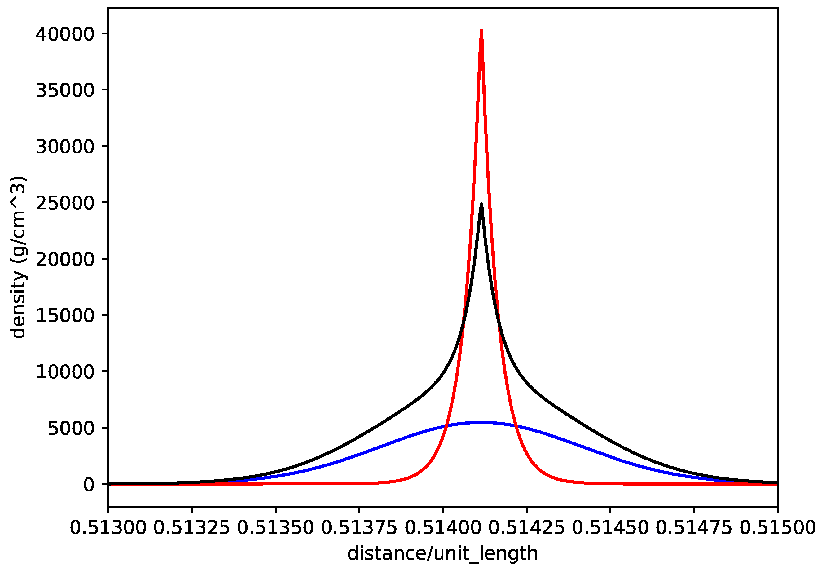
Here, s is the normalized propagation length, $s=x/s_u$, $s_u$ is the unit length defined as $s_u=\left(2E\hslash c\right)/|\Delta m_{31}^2{c}^4|$, $\mathsf{\alpha }=\Delta m_{21}^2/|\Delta m_{31}^2|$, $\gamma =\Delta m_{31}^2/|\Delta m_{31}^2|$, and $A\left(s\right)=2E{V}_e\left(x\right)/|\Delta m_{31}^2|$. The mass differences $\Delta m_{ij}^2$ were taken from Reference [21], and $\gamma =\pm 1$ in Equation (11) takes into account the normal(inverted) mass ordering, $\Delta m_{31}^2>0$($\Delta m_{31}^2<0$). In the calculation, we use a number N of density spikes, entering $A\left(s\right)$ via $V_e\left(x\right)$. Shown in Figure 2 are different density profiles: Gaussians in blue, exponential in red, and a combination of the two of them in black. Each density profile represents the electron density near an atomic nucleus multiplied by twice the proton mass. Given that the Gaussians are normalized to unity, an additional normalization factor ${\rho }_N$ was used to recover the flat average density of matter $\rho$:

$${\rho }_N=\rho s/N,$$

(12)

where, for an easier comparison with solar density, we used the local equivalence between the average electron density $〈N_e〉$ and average mass density $\rho$:

$$\rho =m_p〈N_e〉/Y_e\approx 2m_p〈N_e〉.$$

(13)

We use a similar relation for ${\rho }_N$ related to the normalization of the Gaussian spikes in the electron density. The number of intervals N can be chosen appropriately to describe the large peak values of the Gaussians.

To integrate Equation (8), we used the ZVODE routine from the SciPy ODE package, which implements a complex version of the VODE algorithm [22]. Given that the electron density spikes are extremely narrow, we tried different widths for the density profiles shown in Figure 2. In an attempt to get good accuracy of the solution, we divided the width of each density spike by about 100 integration steps, and required for each step an absolute tolerance of ${10}^{-10}$ from ZVODE routine.

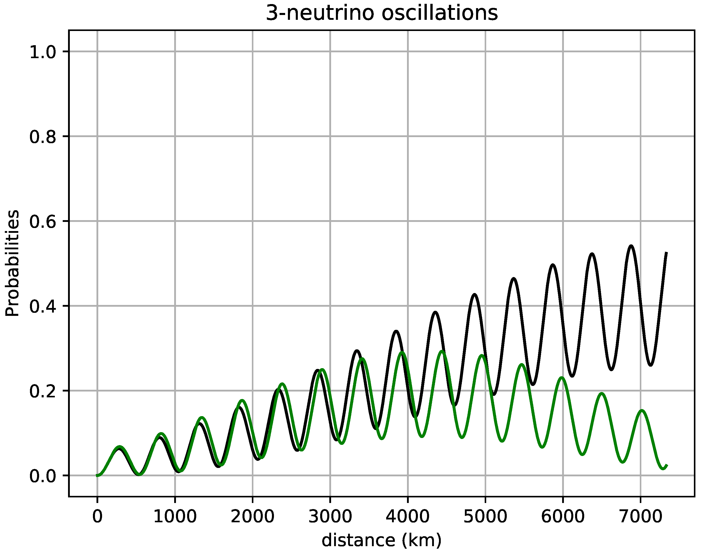
The results in Figure 3 show a significant difference between the solution of the integration method using the spiked density profile (in black) and the “exact” eigenvalues solution corresponding to the equivalent flat electron density (in dark green). As one can see from the figure, there is little effect at 1300 km that corresponds to the Deep Underground Neutrino Experiment (DUNE)/Long-Baseline Neutrino Facility (LBNF) experiment baseline, but it would have been significant for 7330 km, which is the distance between Fermilab and Gran Sasso or that from CERN to Sanford lab in South Dakota. However, when increasing the accuracy in the ZVODE routine to ${10}^{-12}$, the difference between the two curves in Figure 3 disappeared. This situation emphasized once again the danger of relying solely on numerical analysis. In addition, the needed accuracy of ${10}^{-12}$ being close to the numerical round-off error for double precision further emphasizes the difficulty of the numerical problem. We also extensively checked this aspect using Julia’s Differential Equations package, which has a much richer set of routines that can integrate stiff and nonstiff systems of complex differential equations, and the behavior was similar to that we experience with ZVODE.

Therefore, we tried using a more direct analysis to understand this result, which will be presented in the next section.

3. The Iterations Algorithm

Previous work on neutrino oscillation probabilities in matter includes perturbative expansions [20,23,24,25]. The most used approach is to diagonalize the Hamiltonian in matter, and use perturbation theory to identify main contributing terms. In the process, one uses the S-matrix approach for the propagation of the amplitudes. For example, for Equation (11), the corresponding S-matrix is given by:

$$S\left(s\right)=T{e}^{-i{\int }_0^{s}H\left(s^{\prime }\right)d{s}^{\prime }},$$

(14)

where the T operator in front of the exponential indicates an ordered position-dependence of the integrals when the matrix exponential is expanded (similar to the time-ordered product). The S-matrix can be used to calculate the probability of measuring neutrino flavor $\alpha$ at distance s assuming that flavor $\mathsf{\beta }$ was emitted at $s=0$ [23]:

$$P_{\beta \to \alpha }={\left|S_{\alpha \beta }\left(s\right)\right|}^2.$$

(15)

In the case of constant electron density, $A\left(s\right)$ in Equation (11) does not depend on the integration variable s, and one can use the diagonalization methods and/or perturbative expansions [20,23,24,25]. Alternatively, one can directly integrate Equation (11).

Here, we propose using the matrix solution to Equation (11) in a different way: we divide the s interval in N small pieces $\Delta s_i$ (for example, equally spaced $\Delta s_i=s/N$), for which we consider the $H\left(s_i\right)$ Hamiltonian to be constant:

$$H\left(s\right)\equiv U{D}_1{U}^{†}+D_2\left(s\right),$$

(16)

where the diagonal matrices $D_1$ and $D_2$ can be identified by comparing with Equation (11). The solution to Equation (11) can be written as:

$$S\left(s\right)=\prod _{i=1}^{N}S(\Delta s_i).$$

(17)

Given that the $\Delta s_i$ are small, one can show that the matrices $S(\Delta s_i)$ can be approximated by:

$$S(\Delta s_i)=e^{-i\Delta s_i{D}_2\left(s_i\right)}U{e}^{-i\Delta s_i{D}_1}{U}^{†}.$$

(18)

Moreover, given that matrices $D_1$ and $D_2$ are diagonal, then:

$$e^{-i\Delta s_i{D}_2\left(s_i\right)}=\left(\begin{array}{ccc}{e}^{-i\Delta s_i\overline{A}\left(s_i\right)}& 0& 0\\ 0& 1& 0\\ 0& 0& 1\end{array}\right)\equiv U_A\left(s_i\right),$$

(19)

and:

$$e^{-i\Delta s_i{D}_1}=\left(\begin{array}{ccc}1& 0& 0\\ 0& e^{-i\Delta s_i\alpha }& 0\\ 0& 0& e^{-i\Delta s_i\gamma }\end{array}\right)\equiv U_f,$$

(20)

where $\overline{A}\left(s_i\right)$ is calculated with the average electron density in the interval $(s_i,s_i+\Delta s_i)$. Using Equations (17)–(20), one can iteratively find the S-matrix and the associated probabilities of Equation (15). We will call this approach the iterations method. In the proof of Equation (18), one needs the transformations forth and back between the flavor amplitudes and the mass eigenstates amplitudes:

$${\nu }_{\alpha }=\sum _i{U}_{\alpha i}{\nu }_i;{\nu }_i=\sum _{\alpha }{\left(U^{†}\right)}_{i\alpha }{\nu }_{\alpha }.$$

(21)

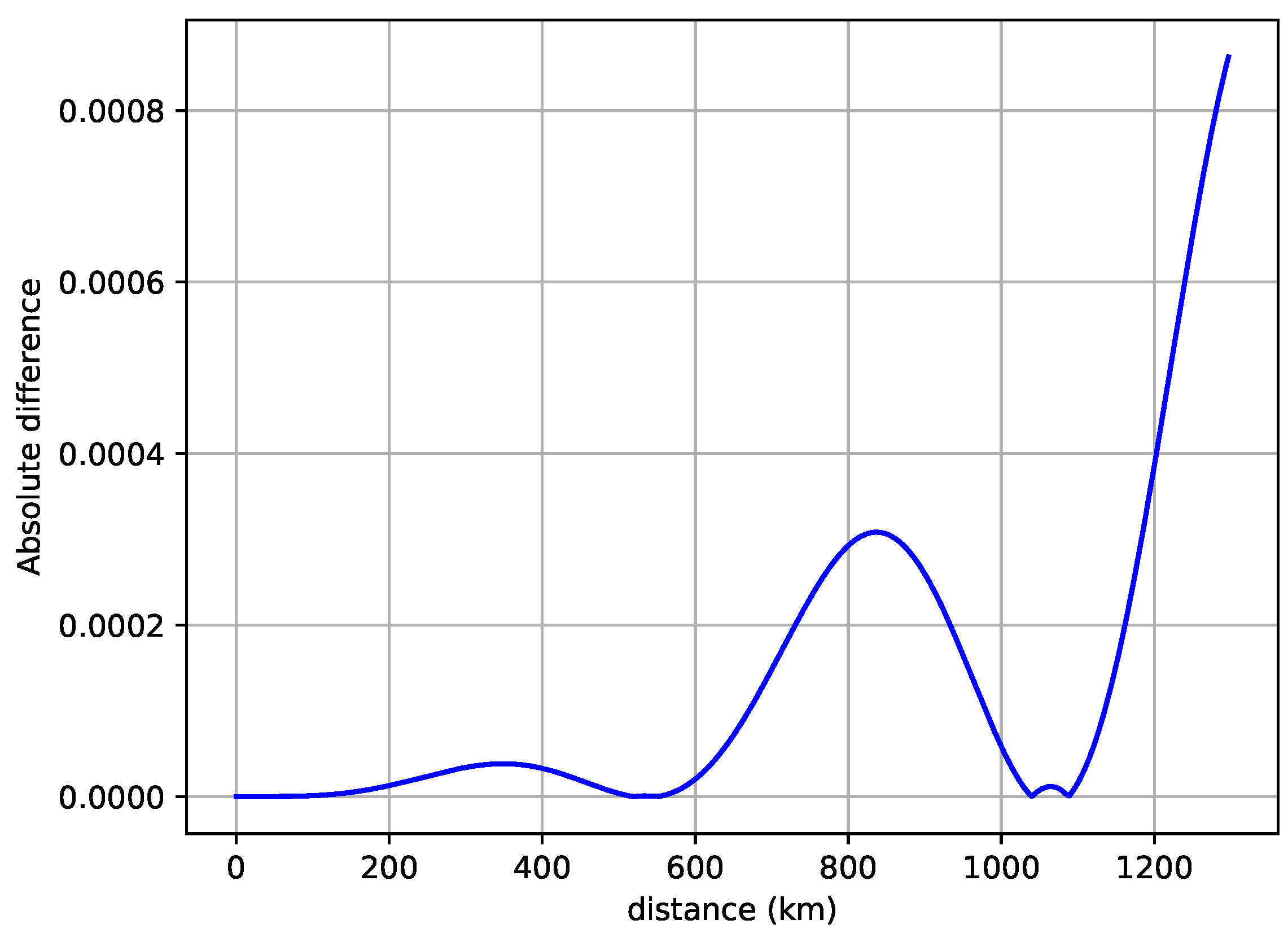
The condition for small $\Delta s_i$ used in Equation (18) suggests that one needs a large number of iterations to obtain good accuracy. Our numerical implementation indicates that even 10–15 factors in Equation (17) would provide a 0.1% accuracy when compared with the “exact” eigenvalues method. Figure 4 shows the difference between the iterations method described above when only 15 iterations are used, and the exact eigenvalues method solution. Increasing N to 150 reduces the absolute difference to less than ${10}^{-5}$.

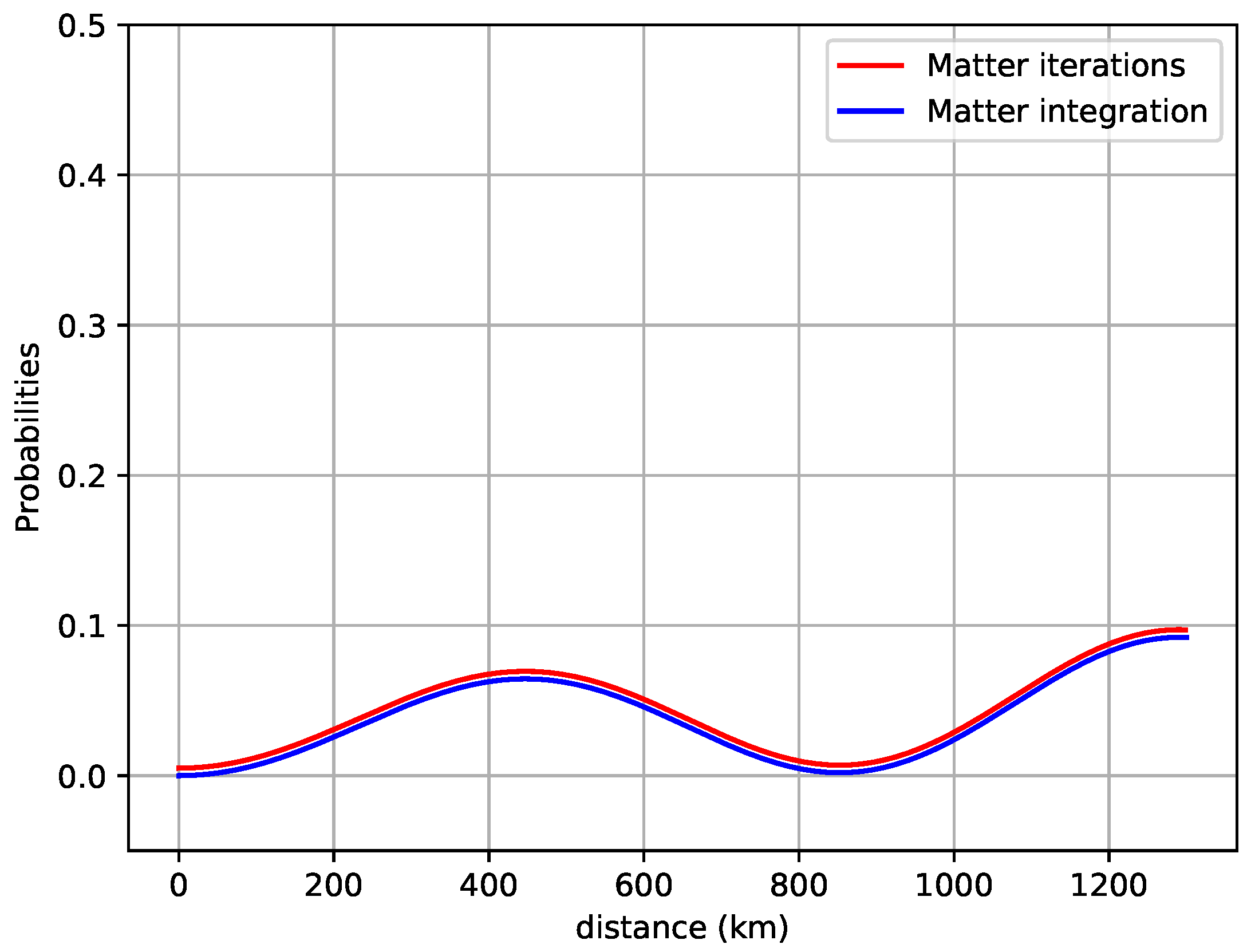
The iterations method described above works as well for smoothly varying average electron (matter) densities. Figure 5 shows the results of the above method (red curve) compared with the solution obtained by directly integrating Equation (8) for a varying density through the Earth’s crust for the DUNE/LBNF experiment, similar to that described in Reference [26] (blue curve). The electron neutrino appearance probability is calculated for a muon neutrino beam of 0.8 GeV. The two curves are overlapping if the artificial 0.005 shift to the red curve is removed (the estimated error used for both algorithms is about $10-5$).

The iterations algorithm is very efficient, while in almost all cases one can use a equally spaced grid ($\Delta s_i=const$), and the product of the matrices $U{U}_f{U}^{†}$ in Equation (18) can be precalculated. Therefore, the right-hand side of Equation (18) can be easily calculated at any iteration step in Equation (17) by multiplying each raw of the precalculated matrix with the corresponding diagonal element in $U_A\left(s_i\right)$ (Equation (19)). One can conclude that the algorithm is very simple and efficient, features that become even more important when it is extended to the light sterile neutrino(s) case (see Section 5). In addition, it is faster than a direct integration method for the case of varying matter densities: in a comparison with the integration algorithm used in Reference [26] (see Reference [19] in [26]) for the same matter density profile used in Figure 5, we observed a factor of 20 less iterations needed, equivalent to a speedup of about 20, under the same accuracy. A simple way of understanding this improvement relative to the direct integration of Equation (11) is that Equation (18) includes some partial integration information through the exponential factors in the diagonal matrices $U_A\left(s_i\right)$ and $U_f$.

4. The Connection to the Integration Method

The iterations algorithm described above can also be used to understand the results of Section 2. To see that, one can consider the electron density in condensed matter composed of N spikes clustered around the atomic nuclei. One can further approximate the spikes with Dirac delta functions, which are normalized to unity and multiplied by the constant given in Equation (12). Then, when integrating Equation (8) on each $\Delta s_i$ segment, one can (i) transform the flavor amplitudes into mass-eigenstate amplitudes with $U^{†}$ (for example, see Equation (21)), (ii) freely propagate the mass-eigenstate amplitudes using $U_m$, (iii) transform the mass-eigenstate amplitudes into flavor amplitudes with U, and (iv) integrate Equation (8) over the Dirac delta spikes. For the last step, one can assume that in the vicinity of a Dirac delta spike only the term proportional with $A\left(s\right)$ in Equation (8) survives:

$$i\frac{d{\nu }_e\left(s\right)}{ds}=A\left(s\right){\nu }_e\left(s\right).$$

(22)

Given that the Dirac delta function norm in Equation (12) is proportionate to $\rho \left(s/N\right)=\rho \Delta s_i$, then $A\left(s\right)=\Delta s_i\overline{A}\left(s_i\right)\delta \left(s\right)$ in the interval $\Delta s_i$, and the solution to the above equation becomes:

$${\nu }_e\left(s_a\right)=e^{-i\Delta s_i\overline{A}\left(s_i\right)}{\nu }_e\left(s_b\right),$$

(23)

where $s_b\approx s_a$ are the s coordinates before and after the delta spike in the $\left(s_i,s_i+\Delta s_i\right)$ interval, and $\overline{A}\left(s_i\right)$ is calculated with the average electron density of Equation (13). Therefore, the result of integrating the full vector of amplitudes over the Dirac delta spikes is:

$$\left(\begin{array}{c}{\nu }_e\left(s_a\right)\\ {\nu }_{\mu }\left(s_a\right)\\ {\nu }_{\tau }\left(s_a\right)\end{array}\right)=\left(\begin{array}{ccc}{e}^{-i\Delta s_i\overline{A}\left(s_i\right)}& 0& 0\\ 0& 1& 0\\ 0& 0& 1\end{array}\right)\left(\begin{array}{c}{\nu }_e\left(s_b\right)\\ {\nu }_{\mu }\left(s_b\right)\\ {\nu }_{\tau }\left(s_b\right)\end{array}\right)\equiv U_f\left(\begin{array}{c}{\nu }_e\left(s_b\right)\\ {\nu }_{\mu }\left(s_b\right)\\ {\nu }_{\tau }\left(s_b\right)\end{array}\right).$$

(24)

Putting together all the steps of the algorithm described above, one gets for the S-matrix factors entering Equation (17):

$$S(\Delta s_i)=U_A\left(s_i\right)U{U}_f{U}^{†},$$

(25)

which is the same as in Equation (18) with the definitions (19)–(20) for $U_A$ and $U_f$. This completes the proof that justifies the use of an average electron density, rather than its large variation around the atomic nuclei. For smooth changes of the average electron density one can use a typical coarse-graining argument.

5. The Case of Light Sterile Neutrinos

Recent short-baseline neutrino oscillations investigation [27] seems to confirm older suspicions that one or more sterile neutrinos may be present. A vigorous short-baseline neutrino program to settle this issue is underway at Fermilab [28]. Therefore, we consider extending our algorithm for neutrino oscillations in varying electron density by including the effect of sterile neutrinos. Here, we consider one sterile neutrino and a fourth mass eigenstate with a mass of about 1 eV. Then, in all above equations, a new sterile flavor with its amplitude ${\nu }_s$ needs to be included, and the $3\times 3$ PMNS mixing matrix $U_3$ should be extended to four rows and four columns (the extension to more sterile neutrino and mass eigenstates is straightforward). One could find compact formulae for the $4\times 4$ matrix elements [20,29], but to avoid typos in the lengthy equations and given that we are mainly interested in numerical calculations, we can obtain the 4-dimensional $U_{3+1}$ matrix using six $4\times 4$ rotations:

$$U\equiv U_{3+1}=U_{34}\left({\theta }_{34},{\delta }_{34}\right)U_{24}\left({\theta }_{24},{\delta }_{24}\right)U_{14}\left({\theta }_{14},{\delta }_{14}\right)U_{23}\left({\theta }_{23},{\delta }_{23}\right)U_{13}\left({\theta }_{13},0\right)U_{12}\left({\theta }_{12},0\right).$$

(26)

Here, ${\theta }_{ij}$ are the mixing angles and ${\delta }_{ij}$ are the CP-violating phases. The $U_{ij}({\theta }_{ij},{\delta }_{ij})$ are $4\times 4$ matrices that represent rotations in two direction, $ij$, such that the $U_{ii}$ and $U_{jj}$ matrix elements are $cos\left({\theta }_{ij}\right)$ and the $U_{ij}$ matrix elements are $sin\left({\theta }_{ij}\right)e^{-i{\delta }_{ij}}$ (the $U_{ji}$ matrix elements being its complex conjugate). Then, Equations (11) and (15)–(20) can be extended using:

$$D_1=\left(\begin{array}{cccc}0& 0& 0& 0\\ 0& \alpha & 0& 0\\ 0& 0& \gamma & 0\\ 0& 0& 0& \kappa \end{array}\right),D_2\left(s\right)=\left(\begin{array}{cccc}A\left(s\right)& 0& 0& 0\\ 0& 0& 0& 0\\ 0& 0& 0& 0\\ 0& 0& 0& B\left(s\right)\end{array}\right).$$

(27)

Here, $\kappa =\Delta m_{41}/|\Delta m_{31}|$ and $B\left(s\right)=-2E{V}_n\left(x\right)/|\Delta m_{31}^2|$, where $V_n\left(x\right)$ given in Equation (6) is proportional with the neutron density in nuclei. Given that the neutron density inside a nucleus is orders of magnitude larger than the electron density at the nucleus, the spikes in $B\left(s\right)$ are much larger than those in $A\left(s\right)$. For example, in typical atoms in the Earth’s, the maximum electron-induced optical potential is about ${10}^{-7}eV$, while the neutron-induced optical potential is about $5$ eV. In addition, the slope of the neutron density in nuclei is much steeper, and the validity of the extension of Equation (11) can only be justified for neutrino energies above 1.5 GeV (see Equation (9)). For those energies, the algorithm of Section 3 can be easily extended using the definitions (26) and (27). Extending the analysis of Section 4, one can conclude that the use of average density in the $A\left(s\right)$ and $B\left(s\right)$ terms entering Equation (27) is granted. Then, the average scaled potentials, $\overline{A}\left(s\right)$ and $\overline{B}\left(s\right)$, are similar in magnitude, and the $U_f$ and $U_A\left(s_i\right)$ matrices in the S-matrix Equation (25) become:

$$U_f=\left(\begin{array}{cccc}1& 0& 0& 0\\ 0& e^{-i\Delta s_i\alpha }& 0& 0\\ 0& 0& e^{-i\Delta s_i\gamma }& 0\\ 0& 0& 0& e^{-i\Delta s_i\kappa }\end{array}\right),U_A\left(s_i\right)=\left(\begin{array}{cccc}{e}^{-i\Delta s_i\overline{A}\left(s_i\right)}& 0& 0& 0\\ 0& 1& 0& 0\\ 0& 0& 1& 0\\ 0& 0& 0& e^{-i\Delta s_i\overline{B}\left(s_i\right)}\end{array}\right).$$

(28)

Using matrices (26) and (28) in the iterations algorithm formula, Equation (25), can be used to calculate the S-matrix and the transition probability.

For neutrino energies lower than 1.5 GeV, the $4\times 4$ extension of Equation (5) needs to be used. In that case, the widely different mass scales would make the analysis intractable. However, if one artificially increases the mass and the potential scales close to the neutrino energy scale, one can directly integrate the $4\times 4$ extension of Equation (5). A preliminary numerical analysis suggests that using average macroscopic electron and neutron densities provides the same oscillation probabilities as using the spiked densities. Alternatively, one can consider the S-matrix for the $4\times 4$ extension of Equation (5) and treat the neutron density spikes around the atomic nuclei as in Section 4 above. This analysis will be reported separately.

Finally, the extension of our algorithm to more light sterile neutrinos, e.g., 3 + 2, is simple and straightforward. One only needs to calculate the $U_{3+2}$ mixing matrix by extending the definition given in Equation (26), and to extend the $D_1$, $D_2$, $U_f$, and $U_A$ matrices, Equations (27) and (28), by adding the appropriate diagonal matrix elements.

6. Conclusions

In conclusion, we analyzed the effect of the large electron density variations around the atomic nuclei on the neutrino oscillation probabilities in condensed matter. This analysis is relevant for the DUNE/LBNF experiment. In Section 2, we attempted to fully integrate the evolution equation for the neutrino amplitudes by considering the large variation of the electron density near the atomic nuclei and therefore that of the neutrino potential. We found that the numerical integration under these conditions could be treacherous, and could lead to erroneous results.

In Section 3 of the manuscript, we proposed a new iterative solution to the neutrino amplitudes evolution equation, which proves to be very fast, reliable, and applicable to either constant matter density or slowly varying matter density (assuming average electron densities). We also showed that this algorithm is simple, efficient, very easy to implement, and it is faster (needs less iterations) by a factor of about 20 than the direct integration algorithm.

In addition, we showed in Section 4 that one can obtain the same iterations method solution, by assuming that the spikes in the electron density around the atomic nuclei can be approximated by Dirac delta functions. Our solution thus justifies the use of average electron densities for matter effects in neutrino oscillation probabilities.

Furthermore, in Section 5, we showed that the new algorithm can be extended to the case where one or more light sterile neutrinos exist. We also showed that for some neutrino energy range relevant for long baseline experimentsm, the neutral current optical potential can be calculated with an average neutron density, rather than the spiked neutron density around the atomic nuclei.

References

- Wolfenstein, L. Neutrino Oscillations in Matter. Phys. Rev. D 1978, 17, 2369. [Google Scholar] [CrossRef]
- Mikheyev, S.P.; Smirnov, A.Y. Resonance Amplification of Oscillations in Matter and Spectroscopy of Solar Neutrinos. Sov. J. Nucl. Phys. 1985, 42, 913. [Google Scholar]
- Smirnov, A.Y. The Mikheyev-Smirnov-Wolfenstein (MSW) Effect. arXiv 2019, arXiv:1901.11473. [Google Scholar]
- Haxton, W.C. Adiabatic Conversion of Solar Neutrino. Phys. Rev. Lett. 1986, 57, 1275. [Google Scholar] [CrossRef] [PubMed]
- Parke, S.J. Nonadiabatic Level Crossing in Resonant Neutrino Oscillations. Phys. Rev. Lett. 1986, 57, 1275. [Google Scholar] [CrossRef] [PubMed] [Green Version]
- Lisi, E.; Montanino, D. Earth regeneration effect in solar neutrino oscillations: An analytic approach. Phys. Rev. D 1997, 56, 1792. [Google Scholar] [CrossRef] [Green Version]
- Blennow, M.; Ohlsson, T.; Snellman, H. Day-night effect in solar neutrino oscillations with three flavors. Phys. Rev. D 2004, 69, 073006. [Google Scholar] [CrossRef] [Green Version]
- Long, H.W.; Li, Y.F.; Giunti, C. Day-night asymmetries in active-sterile solar neutrino oscillations. J. High Energy Phys. 2013, 2013, 56. [Google Scholar] [CrossRef] [Green Version]
- Horoi, M. On the MSW neutrino mixing effects in atomic weak interactions and double beta decays. arXiv 2020, arXiv:1803.06332. to appear in EPJA. [Google Scholar]
- Horoi, M. Neutrinoless Double Beta Decay of Atomic Nuclei. AIP Proc. 2019, 2165, 020012. [Google Scholar] [CrossRef]
- Giunti, C.; Kim, C.W. Fundamentals of Neutrino Physics and Astrophysics; Oxford University Press: Oxford, UK, 2007. [Google Scholar]
- Mannheim, P.D. Derivation of the formalism for neutrino matter oscillations from the neutrino relativistic field equations. Phys. Rev. D 1988, 37, 1935. [Google Scholar] [CrossRef] [PubMed]
- Giunti, C.; Kim, C.W.; Lee, U.W.; Lam, W.P. Majoron decay of neutrinos in matter. Phys. Rev. D 1992, 45, 1557. [Google Scholar] [CrossRef]
- Gonzales-Garcia, M.C.; Nir, Y. Neutrino masses and mixing: Evidence and implications. Rev. Mod. Phys. 2003, 75, 345. [Google Scholar] [CrossRef] [Green Version]
- Smirnov, A.Y. Solar neutrinos: Oscillations or no-oscillations. arXiv 2016, arXiv:1609.02386. [Google Scholar]
- Rata, I.; Shvartsburg, A.A.; Horoi, M.; Frauenheim, T.; Siu, K.W.M.; Jackson, K.A. Single-Parent Evolution Algorithm and the Optimization of Si Clusters. Phys. Rev. Lett. 2000, 85. [Google Scholar] [CrossRef] [PubMed] [Green Version]
- Jackson, K.A.; Horoi, M.; Chaudhuri, I.; Frauenheim, T.; Shvartsburg, A.A. Unraveling the Shape Transformation in Silicon Clusters. Phys. Rev. Lett. 2004, 93, 013401. [Google Scholar] [CrossRef]
- Giannozzi, P.; Baroni, S.; Bonini, N.; Calandra, M.; Car, R.; Cavazzoni, C.; Ceresoli, D.; Chiarotti, G.L.; Cococcioni, M.; Dabo, I.; et al. QUANTUM ESPRESSO: A modular and open-source software project for quantum simulations of materials. J. Phys. Condens. Mater. 2009, 21, 395502. [Google Scholar] [CrossRef]
- Peskin, M.E.; Schroeder, D.V. An Introduction to Quantum Field Theory; Perseus Books: New York, NY, USA, 1995. [Google Scholar]
- Parke, J.P.; Zhang, X. Compact perturbative expressions for oscillations with sterile neutrinos in matter. arXiv 2019, arXiv:1905.01356. [Google Scholar]
- Esteban, I.; Gonzalez-Garcia, M.C.; Hernandez-Cabezudo, A.; Maltoni, M.; Schwetz, T. Global analysis of three-flavour neutrino oscillations: Synergies and tensions in the determination of θ23, δCP, and the mass ordering. J. High Energy Phys. 2019, 2019, 106. [Google Scholar] [CrossRef]
- Brown, P.N.; Byrne, G.D.; Hindmarsh, A.C. VODE: A Variable Coefficient ODE Solver. SIAM J. Sci. Stat. Comput. 1989, 10, 1038. [Google Scholar] [CrossRef] [Green Version]
- Minakata, H.; Parke, S.J. Simple and Compact Expressions for Neutrino Oscillation Probabilities in Matter. J. High Energy Phys. 2016, 1, 180. [Google Scholar] [CrossRef]
- Denton, P.B.; Minakata, H.; Parke, S.J. Compact perturbative expressions for neutrino oscillations in matter. J. High Energy Phys. 2016, 6, 51. [Google Scholar] [CrossRef] [Green Version]
- Denton, P.B.; Parke, S.J.; Zhang, X. Rotations versus perturbative expansions for calculating neutrino oscillation probabilities in matter. Phys. Rev. D 2018, 98, 033001. [Google Scholar] [CrossRef] [Green Version]
- Roe, B. Matter density versus distance for the neutrino beam from Fermilab to Lead, South Dakota, and comparison of oscillations with variable and constant density. Phys. Rev. D 2017, 95, 113004. [Google Scholar] [CrossRef] [Green Version]
- Aguilar-Arevalo, A.A.; Brown, B.C.; Bugel, L.; Cheng, G.; Conrad, J.M.; Cooper, R.L.; Dharmapalan, R.; Diaz, A.; Djurcic, Z.; Finley, D.A.; et al. [MiniBooNE Collaboration]. Significant Excess of Electronlike Events in the MiniBooNE Short-Baseline Neutrino Experiment. Phys. Rev. Lett. 2018, 121, 221801. [Google Scholar] [CrossRef] [PubMed] [Green Version]
- Machado, P.A.N.; Palamara, O.; Schmitz, D.W. The Short-Baseline Neutrino Program at Fermilab. Annu. Rev. Nucl. Part. Sci. 2019, 66, 363. [Google Scholar] [CrossRef] [Green Version]
- Yue, B.B.; Li, W.; Ling, J.J.; Xu, F.R. A new analytical approximation for a light sterile neutrino oscillation in matter. arXiv 2019, arXiv:1906.03781. [Google Scholar]
Figure 1.
Electron density inside a quartz () cell obtained with DFT calculations using Quantum Espresso code [18]. Shown is the electron density (in atomic units) in a plane through the cell that cuts very close to three silicon nuclei (higher peaks), and two oxygen nuclei.
Figure 2.
Profile of the electron density spikes used in the calculations multiplied by the proton mass, for comparison to equivalent matter density, . The horizontal axis represents a small window in the dimensionless parameter s (see text after Equation (11)).
Figure 3.
Calculated for a baseline of 7330 km and muon neutrino energy of 0.5 GeV. The green line is given by a constant matter density approach (g/cm). The black line was obtained by integrating Equation (8), with a precision of /step using an equivalent spiked electron density, and it is shown to be incorrect (see text for details), while the green curve is the correct result.
Figure 4.
Absolute difference between the probability of electron neutrino appearance calculated with the iteration method described in the text and the “exact” eigenvalues method. A constant matter density of g/cm and a muon neutrino beam of 0.5 GeV was used.
Figure 5.
Comparison of the electron neutrino appearance probability, calculated with the iteration method described in the text, and the direct integration method for smoothly varying electron (matter) density (see text for details). The two curves are artificially separated by 0.005 for a better view. A muon neutrino beam of 0.8 GeV was used in the calculations.
© 2020 by the authors. Licensee MDPI, Basel, Switzerland. This article is an open access article distributed under the terms and conditions of the Creative Commons Attribution (CC BY) license (http://creativecommons.org/licenses/by/4.0/).
Share and Cite
MDPI and ACS Style
Horoi, M.; Zettel, A. Effects of Atomic-Scale Electron Density Profile and a Fast and Efficient Iteration Algorithm for Matter Effect of Neutrino Oscillation. Universe 2020, 6, 16. https://doi.org/10.3390/universe6010016
AMA Style
Horoi M, Zettel A. Effects of Atomic-Scale Electron Density Profile and a Fast and Efficient Iteration Algorithm for Matter Effect of Neutrino Oscillation. Universe. 2020; 6(1):16. https://doi.org/10.3390/universe6010016
Chicago/Turabian StyleHoroi, Mihai, and Adam Zettel. 2020. "Effects of Atomic-Scale Electron Density Profile and a Fast and Efficient Iteration Algorithm for Matter Effect of Neutrino Oscillation" Universe 6, no. 1: 16. https://doi.org/10.3390/universe6010016
Note that from the first issue of 2016, this journal uses article numbers instead of page numbers. See further details here.